
Sensitivity of the Wave Field to High Time-Space Resolution Winds during a Tropical Cyclone
by
 , , , and
Laura Pérez-Sampablo
1,*,
Pedro Osuna
1,
Bernardo Esquivel-Trava
1,
Nicolas Rascle
1,2 and
Francisco J. Ocampo-Torres
3 1
Departamento de Oceanografía Física, Centro de Investigación Científica y de Educación Superior de Ensenada (CICESE), Ensenada 22860, Mexico
2
Laboratoire d’Océanographie Physique et Spatiale, IFREMER, CNRS, Université de Bretagne Occidentale, F29280 Brest, France
3
CEMIE-Océano, C.U., Coyoacán, Mexico City 04510, Mexico
*
Author to whom correspondence should be addressed.
Oceans 2023, 4(1), 92-113; https://doi.org/10.3390/oceans4010008
Submission received: 24 September 2022
/
Revised: 9 February 2023
/
Accepted: 10 March 2023
/
Published: 15 March 2023
Abstract
:The impact of the high space-temporal variability of the wind field during the moderate and intense storm stages of a tropical cyclone on the wave field as computed by the numerical model WaveWatch III is investigated in this work. The realistic wind fields are generated by a high-resolution implementation of the HWRF model in the Gulf of Mexico and stored over 15 min intervals. The spatial structure of the wind field computed by HWRF is highly variable in space and time, although its mean structure is very similar to that described for parametric hurricanes already specified in the previous studies. The resulting storm-generated wave fields have a persistent structure, with wave maxima present in the forward quadrants of the storm and in the rear quadrant II. This structure is determined by the strong winds and the extended fetch condition in quadrants I and II, as well as by the translation speed of the storm. When a shorter time interval is analyzed (e.g., a 3 h period, when the storm becomes a category 1 hurricane), the structure of the mean wind field may differ greatly from the mean field calculated with a sufficiently longer period; however, the spatial distribution of the wave field around the hurricane tends to maintain its typical spatial structure. The use of wind fields with reduced time variability (e.g., with a 3 h moving average) does not change the structure of the mean wave field, but reduces the mean wave height values by up to 10%.
1. Introduction
Tropical cyclones (TCs) are extreme low-pressure meteorological systems developed over the tropical oceans [1]. They are characterized by intense winds, irregular trajectories and fast translation speed [2]. Due to their vortex-like structure, the TCs present cyclonic winds which rapidly vary in space and time [3], thus modifying the intrinsic wind field and the eye of the tropical cyclone [4,5]. These events have a direct impact on the generation and evolution of the wave field. During the TCs’ landfall, the wind and wave patterns become even more complex [4,5].
Several works have been made to study the behavior of the wind, the wave field response to a TC using buoys and altimetry measurements [6,7,8,9,10] and the wind field from parametric models and numerical simulations to analyze the features of the wave field [4,11,12], as well as parametric models of the wind field [11,13]. This information has been used to determine the average features of the wind and wave fields during tropical cyclone conditions. So, based on those results, it has been observed that the strongest winds are located to the right of the eye of the TCs, with respect to its translation movement; whereas, the weakest winds are found to the left of it [6,8,11,14]. This asymmetry emerges as a consequence of the TC curvature [4,14,15,16]. Moreover, the spatial distribution of the mean significant wave height () shows large values to the right of the TC with respect to its propagation direction [4,6,9,10] and, when compared to the wind field, the spatial distribution of mean also exhibits a higher asymmetry [10].
A common way to estimate the mean wind field for the analysis of waves during TCs, with a regular time and space distribution, is through the use of global numerical models. Nonetheless, these fields are not correctly solved by the global atmospheric circulation models, mainly because the wind field during a TC is a relatively small vortex [17]. In other studies, more realistic wind fields are built with higher time resolution by combining wind fields from both reanalysis and hurricane models as the HWIND [12]. The wind fields from HWIND are obtained from the NOAA/HRD [18] and are constructed with information obtained from buoys and ships, as well as from TC reconnaissance aircraft. The wind fields have a 6 km × 6 km resolution, thus covering an 8 × 8 region around the hurricane center, and also have a time resolution of 3 or 6 h. Another wind model used in the study of hurricanes is the Holland parametric model [19]. This model generates a simple vortex, and the wind field is then generated from a radial pressure profile representation of a TC to obtain a symmetrical wind field which, once the translation velocity is incorporated, approaches an asymmetric field characteristic of a tropical cyclone. By contrast, there are atmospheric models with physical parameterizations and specific schemes for hurricanes, which are initialized so that the initial state of the model’s atmosphere contains a realistic cyclonic vortex with features closely resembling the observations [20]. The MM5 (Fifth Generation Mesoscale Model [21,22] is among these models. However, the lack of a refinement scheme for the vortex-following grid makes the high-resolution integration (lower than 5 km grid spacing) unrealistic for periods of a few hours [23]. Another commonly used atmospheric model is the WRF-NMM (Non-hydrostatic Mesoscale Model), by which it is possible to follow a vortex and to obtain a better simulation of the TC. Nonetheless, the corresponding vortex wind profile is generated from an analytic Rankine model [20]. Objectively, to simulate the behavior of the TCs with more exactitude, vortex formation schemes with realistic intensity and positioning are needed since this directly affects the trajectory, wind intensity and pressure errors [24]. On the other hand, to simulate wind waves during extreme events such as the tropical cyclones, it is recommended to use as an atmospheric forcing agent—a wind field with high resolution in time and space [25].
Since a high spatial resolution is required to adequately simulate the wind field during TCs, some novel nesting techniques of mobile grids have been incorporated into the models, thus allowing them to register the evolution of the wind field structure during tropical storms and hurricanes. The HWRF atmospheric model is a good example in which the user can obtain high-resolution wind fields throughout space and time around the TCs, besides from monitoring the cyclone trajectory. The high resolution is essential too if we wish to capture the small-scale structures observed in the surroundings of the cyclone’s eyewall, where strong wind velocity gradients are present [17]. This, in turn, may have an important effect on the description of the wave field evolution [25].
Moon et al. [4] provided one of the first attempts to simulate the directional wave spectra under hurricane conditions by using high-resolution winds. In their work, wind data from the NOAA National Hurricane Center (NHC) were used to generate 30 min wind fields, which were used as a forcing to the spectral wave model WAVEWATCH III (WW3). Their results show that the high-resolution wind forcing, as well as the generated wave field, have a dependence on the radius of maximum wind and the cyclone’s translation speed. When the translation speed is low, the wave direction is determined by the distance to the center of the storm; whereas, with high translation speed the dominant waves are rather determined by an effect of prolonged wave exposure to the forcing wind (extended fetch). Thus, the waves in the right quadrants of the cyclone are exposed to the wind for a longer period, remaining trapped within this region.
In a recent study, [26] a high spatial resolution model that includes an atmosphere-wave-ocean coupling has been used. They study the impact of the previously referred interaction in the modeling of the wind-wave field structure during hurricane Bejisa (2014), west of the Indian Ocean, and show the complexity of the wind field structure obtained from their numerical experiment. In the present study, the atmospheric model HWRF is used to obtain realistic wind velocity fields of the tropical cyclone Isaac (2012), with high spatial and time resolution. Based on the numerical results, the spatial structure of the average wind field and the corresponding time variability are analyzed. These winds are used as a forcing to the spectral wave model WW3, so the impact of the TCs’ time variability in the evolution of the space-time structure of the wave field can be analyzed. This paper is organized as follows: In Section 2, the general description of the simulated TC is presented together with the main features of the implemented numerical models and the corresponding parameterizations. Within Section 3, model results validation is described through the analyses of the simulation results and the measurements from buoys. Finally, the conclusions are given in Section 5.
2. Materials and Methods
2.1. Selected Event: Tropical Cyclone Isaac (2012)
The tropical cyclone Isaac evolved from tropical depression to a category 1 hurricane between 21 August and 1 September 2012, most of the time traveling through the Caribbean Sea and the Gulf of Mexico. Its transit across the Gulf of Mexico (GoM) took place during 27–29 August 2012. Isaac arrived at the GoM as a tropical storm between Florida and the northern coast of Cuba, thus traveling towards the northeast with sustained winds of about 26 ms. At the beginning of 27 August, its displacement to the open sea in the GoM was slow, northeastward and remaining as a tropical storm. The subsequent evolution of Isaac was characterized by strong winds and a ring of organized deep convection bordering the eye of the storm. Isaac continued to strengthen gradually and, around 1200 UTC of 28 August, it reached a category 1 hurricane according to the Saffirt–Simpson scale. Finally, at 0000 UTC of 29 August, Isaac made the first landfall at the coast of Louisiana with maximum sustained winds of approximately 36 ms (https://www.nhc.noaa.gov/data/tcr/AL092012_Isaac.pdf accessed on 22 September 2022).
2.2. Model Configuration
2.2.1. Hurricane Dynamic Atmospheric Model
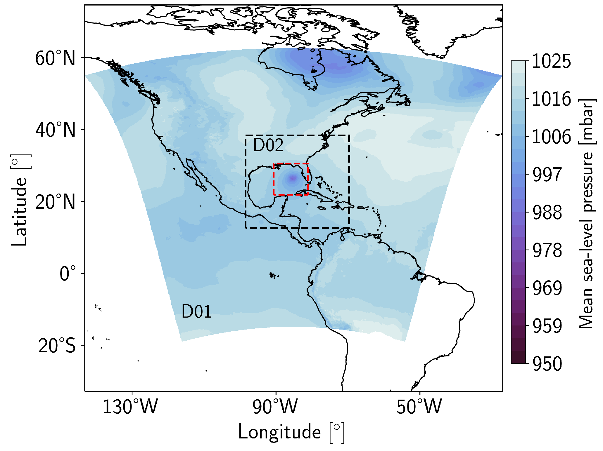
The wind field for hurricane Isaac was obtained using the atmospheric model for hurricanes HWRF version 3.8. This model is a specialized version of the Weather Research and Forecasting (WRF) model, which is focused on ocean–atmosphere interactions [27]. This model solves the dynamic equations over an Arakawa E-grid using a hybrid sigma vertical coordinate system, also possessing the capability of using data assimilation and specific procedures for the relocation of the main vortex. The coverage and resolution of the grids used for the present implementation are shown in Table 1 and Figure 1. Further details on the features and formulations of the HWRF can be found in Gopalakrishnan et al. [28] and Biswas et al. [27].
In this work, HWRF is set up to use the physical parameterizations indicated in Table 2. Although the HWRF model is able of coupling ocean-atmosphere systems, neither ocean coupling nor assimilation is considered here. As initial and boundary conditions for the domain D01, historical data from the NCEP FNL dataset (Research Data Archive: NCAR (https://rda.ucar.edu/datasets/ds083.3/dataaccess/ accessed on 22 September 2022) are used, with space and time resolution equal to 1.0 degree and 6-hourly, respectively. The D02 and D03 mobile grids are initialized using the corresponding downscale variables from the parent domain mean while vortex characteristics (i.e., location, size, intensity and structure), provided by NHC (TCvitals files), are incorporated during the run. The hurricane simulation was carried out from 26 August at 00 UTC, and the model run was set for a 120 h period. The results of the simulation were recorded with 15 min intervals.
2.2.2. Waves Spectral Model
WaveWatch III® (WW3; [33]) is a third generation model operated by the National Oceanic and Atmospheric Administration (NOAA), together with the National Centers for Environmental Predictions (NCEP). The model WW3 describes the evolution of the wave directional spectrum based on the numerical solution of the spectral action balance equation. Most of the results analyzed here refer to a TC developed over deep waters. Under these conditions, the evolution of the directional spectrum is mainly controlled by three processes: the energy transfer between the atmosphere and the waves (wind input), the energy dissipation by deep water wave breaking (whitecapping) and the resonant quadruplet wave–wave interactions. This is treated in our model configuration using the ST6 package (see Table 3).
The governing equation is solved using a regular grid placed over the GoM between 18 N and 31 N, and between 79 W and 98 W (Figure 2a). The time steps used in this implementation are shown in Table 3, and they are chosen taking into account the spatial and spectral discretization, so the CFL criteria is fulfilled. The bathymetry data were obtained from GEBCO (General Bathymetric Chart of the Oceans). In this implementation, data from boundaries are not taken into account because the predominant waves over the region during the analyzed period are those generated by the TC. In order to generate the initial conditions, the model is implemented over a 3-week period using wind information from the ERA5 reanalysis database. Then, starting from 26 August at 00 UTC, the model is forced using wind data from the HWRF output. The results of the WW3 are then recorded with a time interval of 15 min.
3. Results
3.1. Characteristic Parameters of the TC
As mentioned above, the main objective of this paper is to determine and study the average features and time variability of the wind and wave fields during the occurrence of a TC numerical analysis. Hence, it is necessary to confirm that the results provided by the model are adequate by means of a qualitative and quantitative inspection. The validation is performed with information from different databases. From the NHC and HURDAT datasets, the following parameters of the TC were obtained: minimum pressure in the eye of the TC (), intensity of the maximum sustained wind () and the radius of maximum wind (). All these data are available at the 6 h sampling interval. From the operative buoys of the NDBC (National Data Buoy Center), the wind speed at 10 m, , and the significant wave height, , were used.
3.1.1. Structure and Trajectory
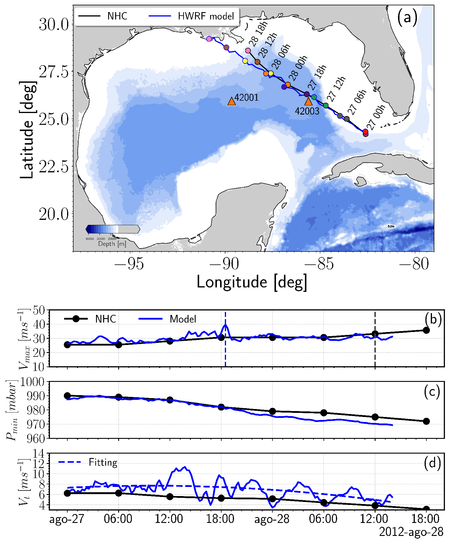
Historically, and , as well as the position of the storm center are considered as key parameters to describe the TC and its evolution. These parameters are also used to evaluate the atmospheric model’s ability to reproduce the TC’s main features. Results from domain 3 (see Table 1) simulated with the HWRF model are compared to the trajectory (Figure 2a, blue line) and characteristics reported by NHC (black line). It is possible to observe that both trajectories are similar. Nonetheless, the storm translation speed, simulated with the HWRF model is higher than the observations. The values computed by the HWRF and those reported by the NHC are shown in Figure 2d. A similar behavior on the trajectory and translation speed of hurricane Isaac is reported by Curcic et al. [37]. The simulated by the model (Figure 2b) shows high variability along the TC trajectory, particularly during the tropical storm stage, whereas those values from the NHC are typically smooth. During the first 18 h of simulation, the computed with the HWRF is slightly higher than reported by the NHC. According to the numerical results, the hurricane category is achieved during 28 August at 18:30 UTC (segmented line in Figure 2b), reaching maximum winds of 39.6 ms. In contrast, according to the NHC report, the category of hurricane was achieved during 28 August, at 12:00 UTC presenting of 33.4 ms with an increasing tendency. This tendency is well reproduced by the model. During the tropical storm stage, the values determined by the HWRF model are very similar to those reported by the NHC (Figure 2c). A clear decreasing tendency is observed, which induces an intensification of the storm and further transition from tropical storm to hurricane. Once this category is reached, the values reported by the NHC tend to decrease, as well as those from the HWRF. As for the values computed with the HWRF (Figure 2d, solid blue line), very high variability is observed in contrast to the NHC time series. Additionally, the TC simulated by the HWRF model travels about 2 ms faster than those reported by NHC. However, it is possible to observe an interesting feature within the values given by the model: the decreasing tendency of the instantaneous values of is highly correlated to the reported information.
3.1.2. Fixed Observations
Recordings of and from two NDBC fixed buoys (42001 and 42003) encountered in the surroundings of the TC trajectory were used for additional validations. In order to evaluate the performance of the model, three statistical parameters were used:
- (a)
- The determination coefficient,where indicates the covariance between the observed data, x and the model results, y; whereas, and indicate their corresponding standard deviation.
- (b)
- The root mean squared error (),and
- (c)
- Bias,where is the average value obtained from the model results, and is the average value from the observation.
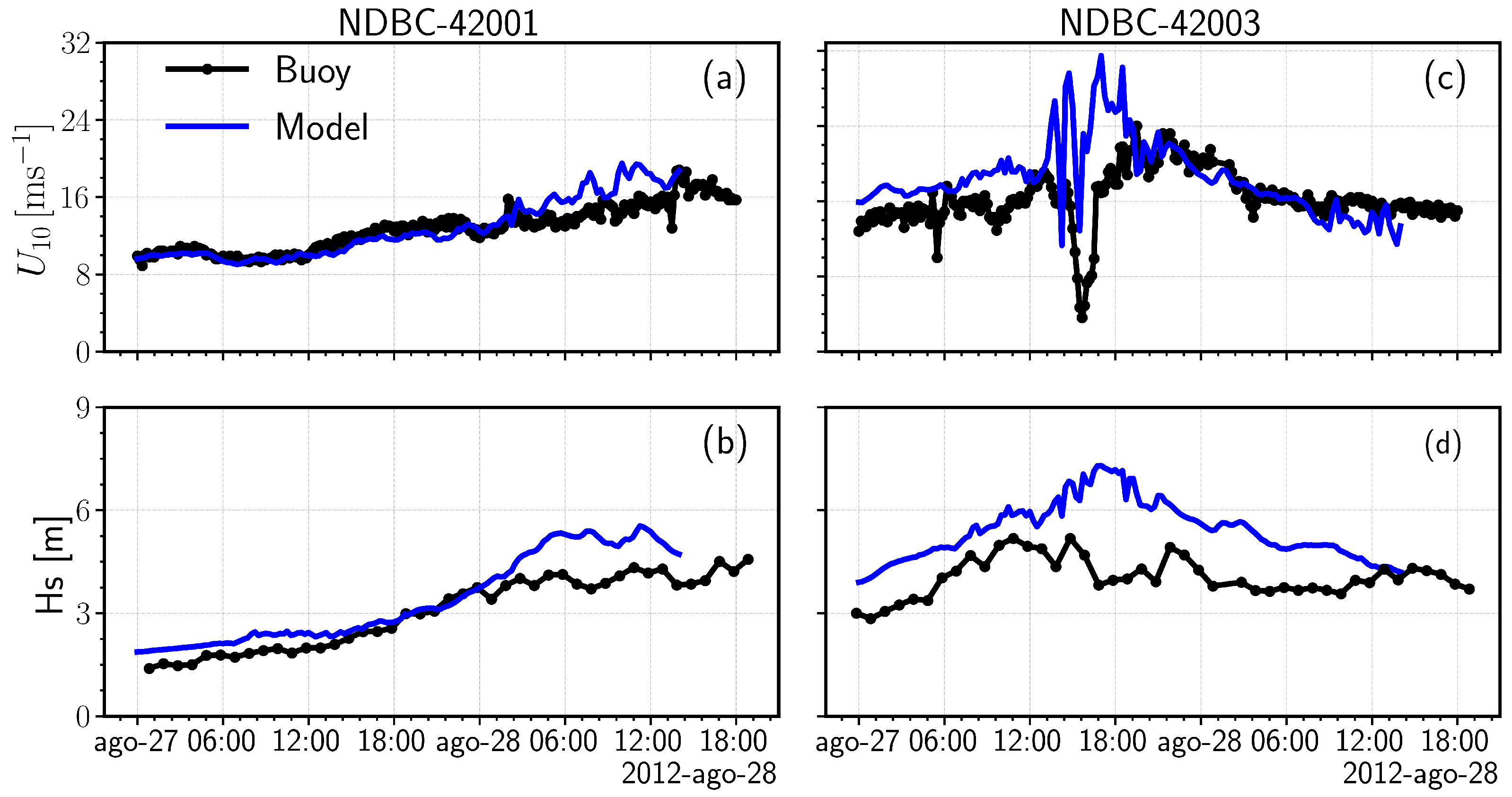
Due to the difference between the observed and computed TC track, the position of the buoy relative to the storm eye may significantly vary. So, the comparison between wind and wave data from buoys 42001 and 42003 was made against the model results for the same relative positions as the one reported by the NHC. The buoy 42001 is located near the central GoM, at 893925 W and 255631 N (see Figure 2a). At some point, the shortest distance between this buoy and the hurricane’s eye was about 200 km, over their left quadrants. In Figure 3a, we show the comparison between the wind intensity observed with the buoy (black line) and those values computed by HWRF (blue line). The model adequately reproduces the observed values until 28 August, then the model results tend to overestimate the values measured by the buoy. An objective comparison between the observations and the model (Table 4) yields an = 0.75, with a of 0.98 ms and a bias of S = −0.22 ms. The overestimation in the wind intensity is reflected in the larger values computed by WW3 with respect to those measured by the buoy (see Figure 3b). In this case, a relatively high of 0.85 is computed with an of 0.5 m and an S = 0.32 m.
The buoy 42003 is located at 853653 W and 255531 N (Figure 2a). The shortest distance between this buoy and the hurricane’s eye is approximately 50 km, over its left quadrants. Figure 3c shows the comparison between the buoy (black line) and the HWRF model (blue line) data for the wind intensity values. The closest approach between the buoy and the eye of the TC was around 16:00 UTC of 27 August, when the buoy reported a wind intensity minimum. During the following 4 h, the buoy shows increasing wind intensity, until reaching a maximum of 26 ms, likely associated with the storm intensification. Then, values from the buoy tend to decrease to about 16 ms; whereas those from the HWRF model are clearly overestimated (up to 10 ms). As observed from the modeled time series, higher variability is depicted in comparison to the buoy observations, probably due to differences in the calculation of the eye size at those specific times. According to HWRF results, the intensification of the registered winds is noticeably higher than the observed, but the decreasing tendency is similar. The values of computed by HWRF at the vicinity of the storm eye indicate a model tendency to overestimate its magnitude, which is also consistent with the translation speed overestimation [38]. This, in turn, would explain the tendency of the WW3 to produce much higher values at the relative position of the buoy. The objective comparison between the model results and observations is not as good as that of buoy 42001. As for the HWRF values, the computed determination coefficient is = 0.2, having a of 5.4 ms with a S = 3.2 ms. Finally, for the computed with the WW3, = 0.47 with a of 1.7 m and a bias of 1.5 m. It is clear that the model does not reproduce the exact evolution of the TC, although it can be seen that the model results tend to reproduce the general pattern observed in the measurements.
3.2. Effects of the Time Resolution of the Wind Field on the Wave Field
The numerical results obtained from the HWRF model show a very high temporal variability, characterized by abrupt changes in the spatial structure of the wind field. According to Janssen [39], good quality of wind data is essential to improve the performance of the wave models and, when it comes to extreme events such as a TC, this fact becomes more relevant [40]. With poor time and space resolution, the wind models may underestimate the wind behavior, particularly at the storm center [41], thus inefficiently representing the wave field evolution. Tolman and Alves [25] also emphasize the relevance of a high time resolution in the characterization of the wind field. In order to analyze the effect of the temporal variability of the wind field on the wave spatial structure computed by WW3, two experiments are performed: one with the wind fields originally calculated by the HWRF model and the other with the same original wind fields but filtered using a 3 h running average. Both wind fields are fed to the wave model with a time resolution of 15 min. The wind data are grouped as a function of [10] and divided into two stages: moderate storm, when > 980 mbar; and the intensification stage, when ≤ 980 mbar (Figure 2c). Prior to the calculation of average values, the instantaneous fields are normalized with their corresponding maximum value. The wind and wave fields are analyzed following the standardization procedure proposed by Young [14]. The procedure consists of normalizing the space dimension with the computed for each field and rotating it along the TC direction of propagation. This procedure allows the positive y-axis to be aligned with the direction of advancement, thus permitting a spatial discretization of the TC parameters into quadrants. The front quadrants of the TC are labeled as I (right) and IV (left), whereas the rear quadrants are identified as II (right) and III (left).
3.2.1. Average Wind and Fields
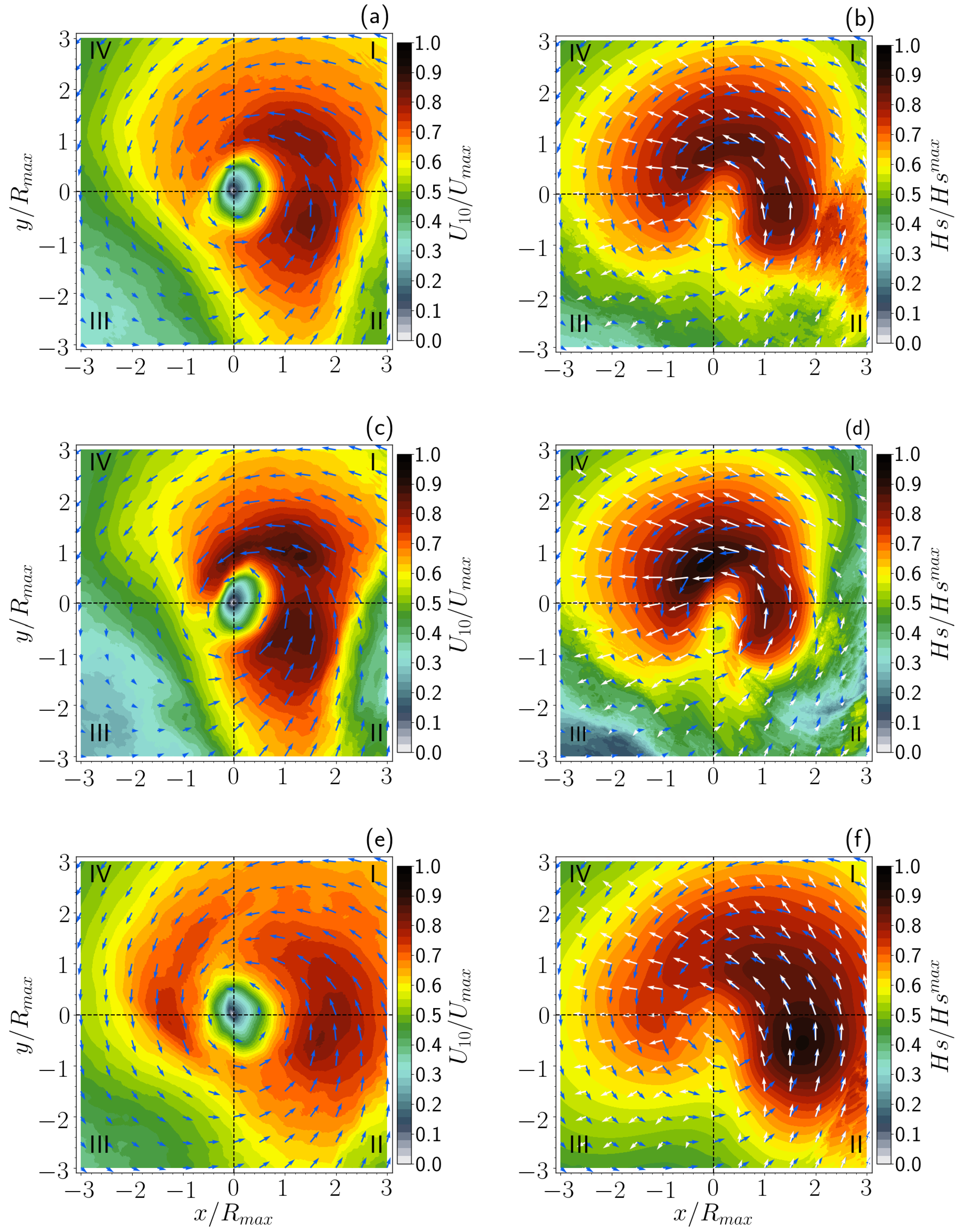
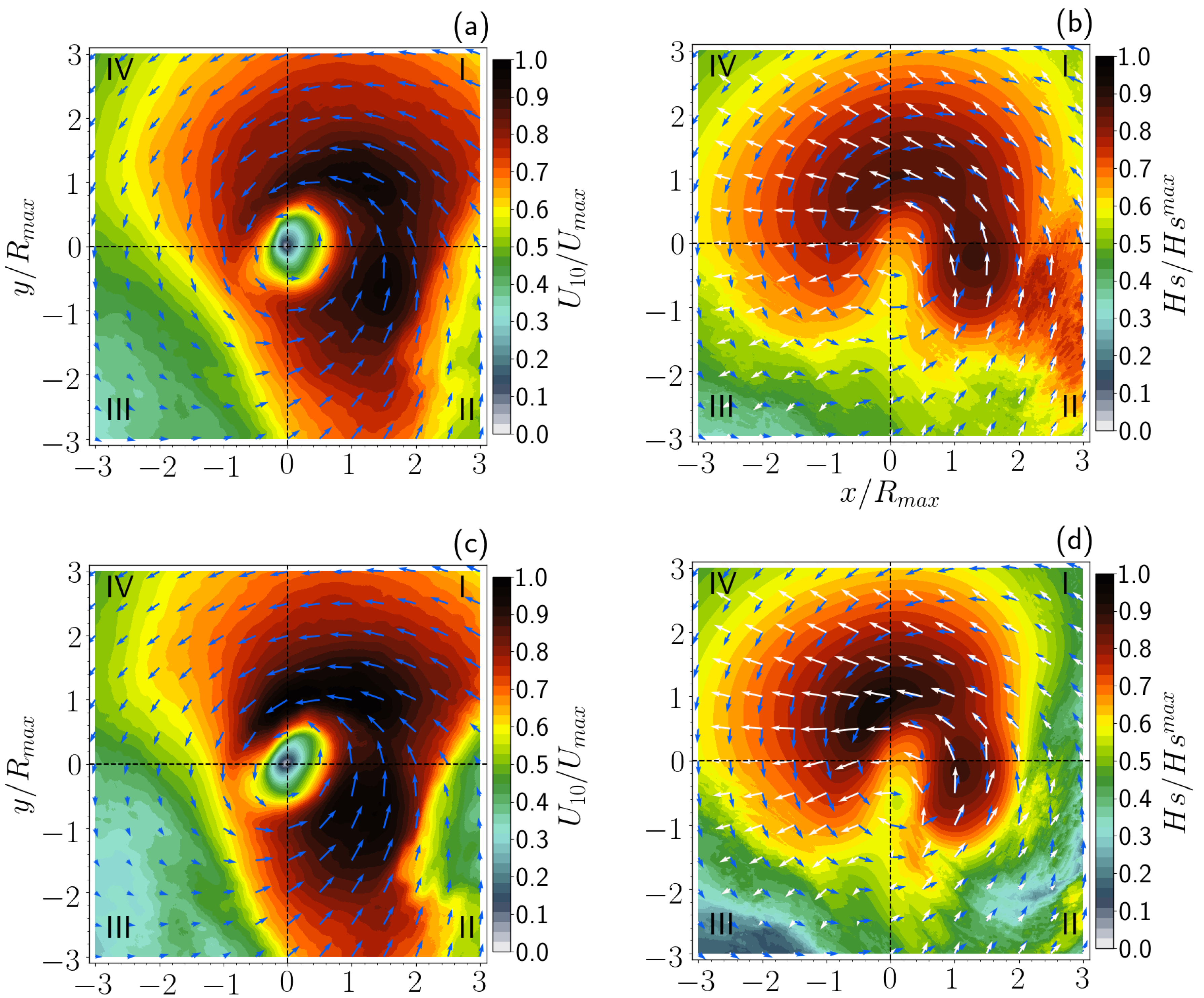
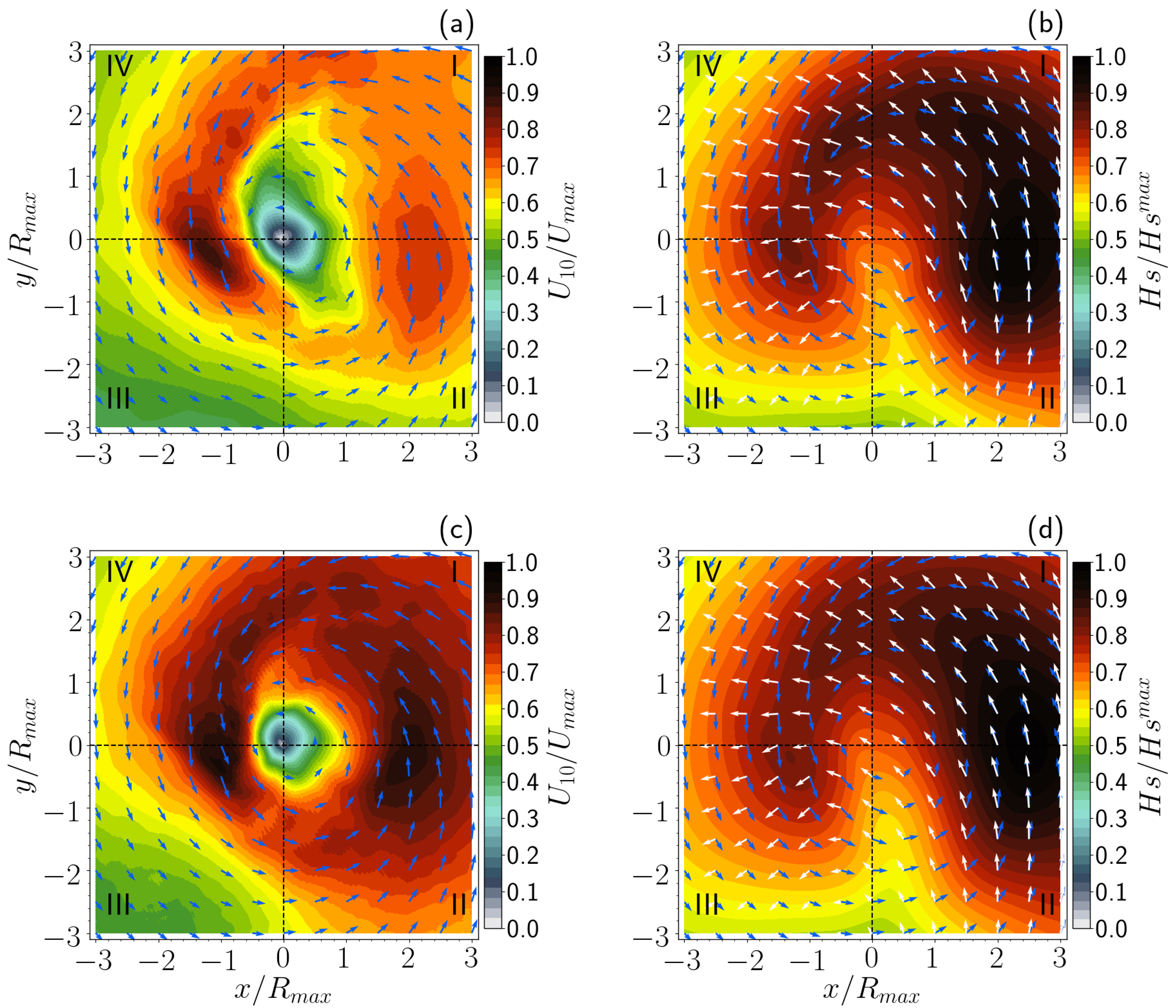
In this section, the full-resolution wind fields computed by HWRF and the corresponding wave fields calculated by WW3 are analyzed. Figure 4 shows the mean wind field considering the full time period (18 h), moderate storm (9 h) and storm intensification stage (9 h) (Figure 4a,c,e, respectively). In general, the wind field presents a clearly-defined storm eye, which is typical from a well-developed storm. Generally, in the 18 h average (Figure 4a) and moderate storm stage (Figure 4c) an asymmetric behavior of the wind field is observed, with the quadrants I and II presenting the higher mean values. In addition, the wind maximum is present to the right of the eye, with strong winds distributed over I and II quadrants, between 1 and 2; these strong winds are readily apparent in these quadrants and between 1 and 2 during the 9 h moderate storm stage analyzed (Figure 4c). Large intensity values are obtained in quadrant IV during the full period 18 h average. It is possible to observe large mean wind values in regions further away from the storm center distance large than 1 in quadrants I and II. This behavior is reported by Esquivel-Trava et al. [9] in quadrant II, and they associated it with the presence of concentric walls in the hurricane. The spatial pattern observed in Figure 4c could be associated with the spatial variability of the spatial structure of the hurricane simulated by HWRF, as well as to the possible presence of concentric walls, although a more detailed analysis is needed to further confirm this statement.
Furthermore, the left quadrant (III), as observed in the 18 h average and during the moderate storm stage (Figure 4c), is characterized by the presence of lower mean wind values. This asymmetry is caused by the cyclonic motion of the storm. Particularly, over the right quadrants, the translation speed of the TC is added to the wind speed near the storm eye vicinity, which allows wind intensification over this region [4,42]. This mean pattern is similar to previous observations from Young [14], Esquivel-Trava et al. [9] and Tamizi and Young [10] using in situ measurements, and it is also similar to simulations from Moon et al. [4], Hu and Chen [43] and Mora Escalante [44]. During the intensification stage (Figure 4e), the asymmetry of the wind field is reduced and moderate mean winds are present over the left quadrant (III and IV) at 1.
In Figure 4b,d,f, the mean fields are presented as obtained from the corresponding averaged wind field (Figure 4a,c,e). During the 18 h intervals (Figure 4b), moderate storm (Figure 4d), intensification stages (Figure 4f), and the greatest mean values are observed to the right of the storm’s eye, in quadrants I and II, at 1. Nonetheless, high mean values are observed in left quadrant IV (Figure 4d) over a region which extends up to 2. The high mean values in quadrants I and II (Figure 4b,d,f) are consistent with the high values observed in Figure 4a,c,d. These results are in agreement with those reported by Moon et al. [4], Esquivel-Trava et al. [9], Liu et al. [11] and Tamizi and Young [10]. In all panels of Figure 4, the mean direction of the wind (blue arrows) and waves (white arrows) are included. Over the right quadrants (I and II), where the wind maxima are observed, wind and waves have nearly the same direction. The difference between them increases in the regions further away from the storm center. Over these quadrants, near the storm eye, the wind waves tend to be local, i.e., actively forced by winds [45]; although Holthuijsen et al. [8] mention that young swell traveling in the same direction as the storm may be present. Away from the regions of maximum winds, the difference between the mean direction of the wind and waves increases, mostly because the waves over these regions are predominantly non-local (swell). As for the left quadrant (III and IV), the waves propagate following a straight line to the right of the wind direction, and they form an angle near to 90. This quadrant is dominated by previously generated waves and has features different from the local wind [45]. Holthuijsen et al. [8] define this kind of pattern as crossing swell (quadrant IV) and opposing swell (quadrant III). In general, these features of the wind and waves’ direction are in accordance with observations [8,9] and numerical model results [4]. It is worth noting that an important feature of the averaged wave field is the position of the minimum , which lies approximately 0.5 south (according to the storm track) of the eye location. This feature is similar to the spatial structure shown by Moon et al. [4] in their Figure 8c, although its cause is not discussed. We can argue that this feature is produced by the translation speed of the storm and the response time of the wave field to the forcing; however, its precise cause needs to be investigated.
3.2.2. Mean Fields of Filtered Winds and the Corresponding Wind Waves
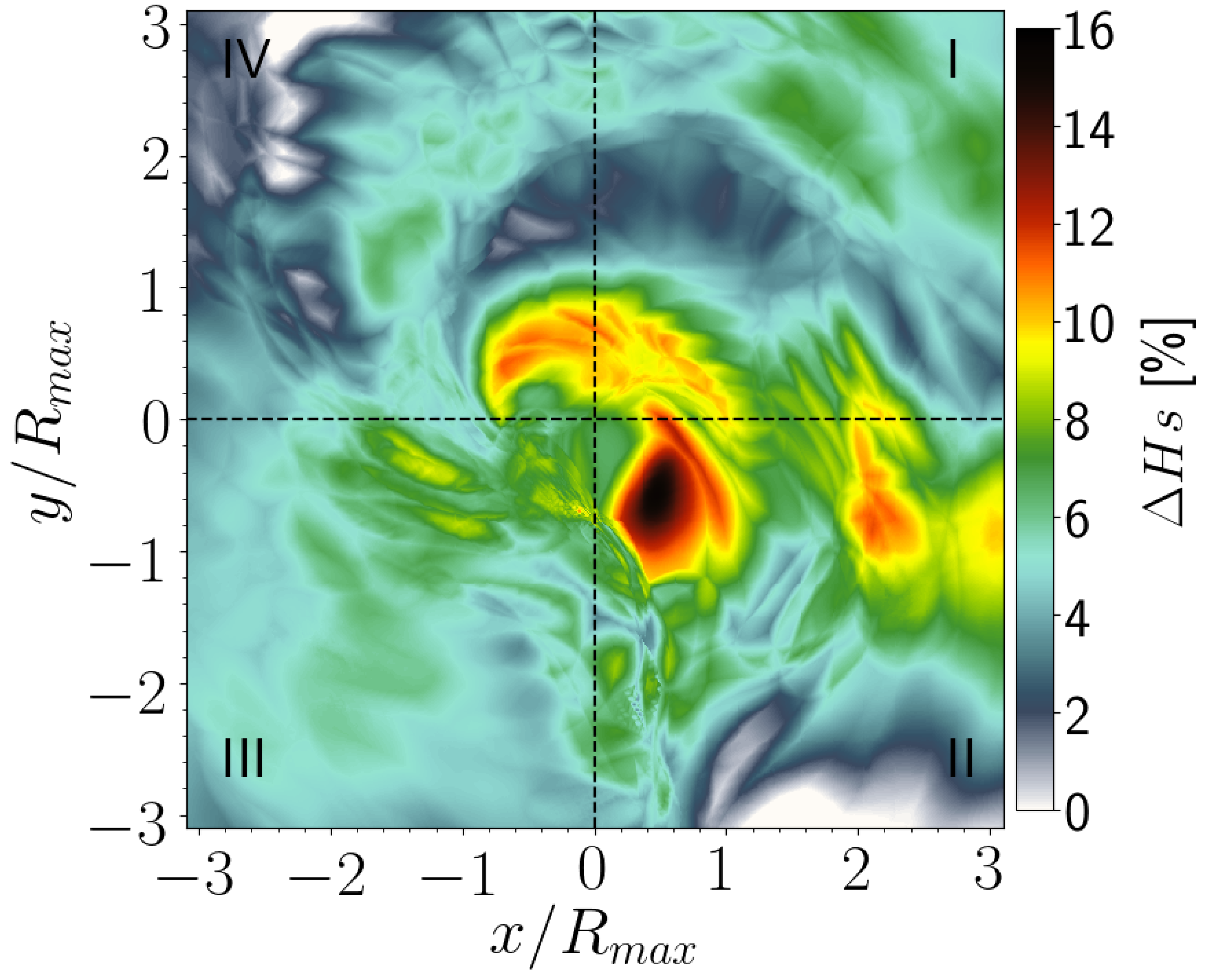
Tolman et al. [41] suggest using data with high spatial resolution in order to get better estimations of the wave field, and particularly to avoid wind underestimation near the storm core. Filtered data with a 3 h running mean were used in order to analyze the effect of low time resolution in and , although the 15 min interval was maintained. In general, the filtered wind fields (Figure 5a,c,e) show a similar spatial pattern to that obtained when the original fields (Figure 4a,c,e) are used. The average values of the filtered wind fields are closer to one, which is the result of their lower spatial variability and slightly lower instantaneous maxima (about 3 ms) than those calculated using the original HWRF results. The mean fields calculated with the filtered wind (Figure 5b,d,f) have a very similar spatial structure to that of the mean fields calculated with the original wind fields. However, the values calculated with the latter wind data tend to be higher than those calculated with the filtered wind data. This difference is most obvious during the intensification stage of the storm when the computed by the model reaches values greater than 9.5 m. Figure 6 shows the average spatial distribution of the differences between the 97.5 percentile values of the calculated using the original winds minus those calculated using the filtered winds. The differences are reported in percentages with respect to the values calculated using the original winds. It is possible to observe that the large values of computed using the original winds are up to 15% higher than those calculated with the filtered wind data. The largest differences are observed in the region around the storm eye wall, mainly in quadrants II and quadrants I and IV. As will be shown in Section 3.3, it is in this region that the greatest temporal wind variability is observed. This type of result is in agreement with the fact that high wind variability influences high values [46].
3.2.3. Particular Case: Change from Tropical Storm to Hurricane
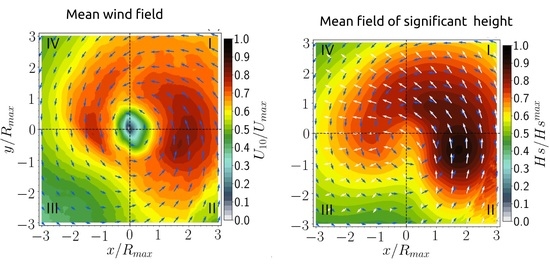
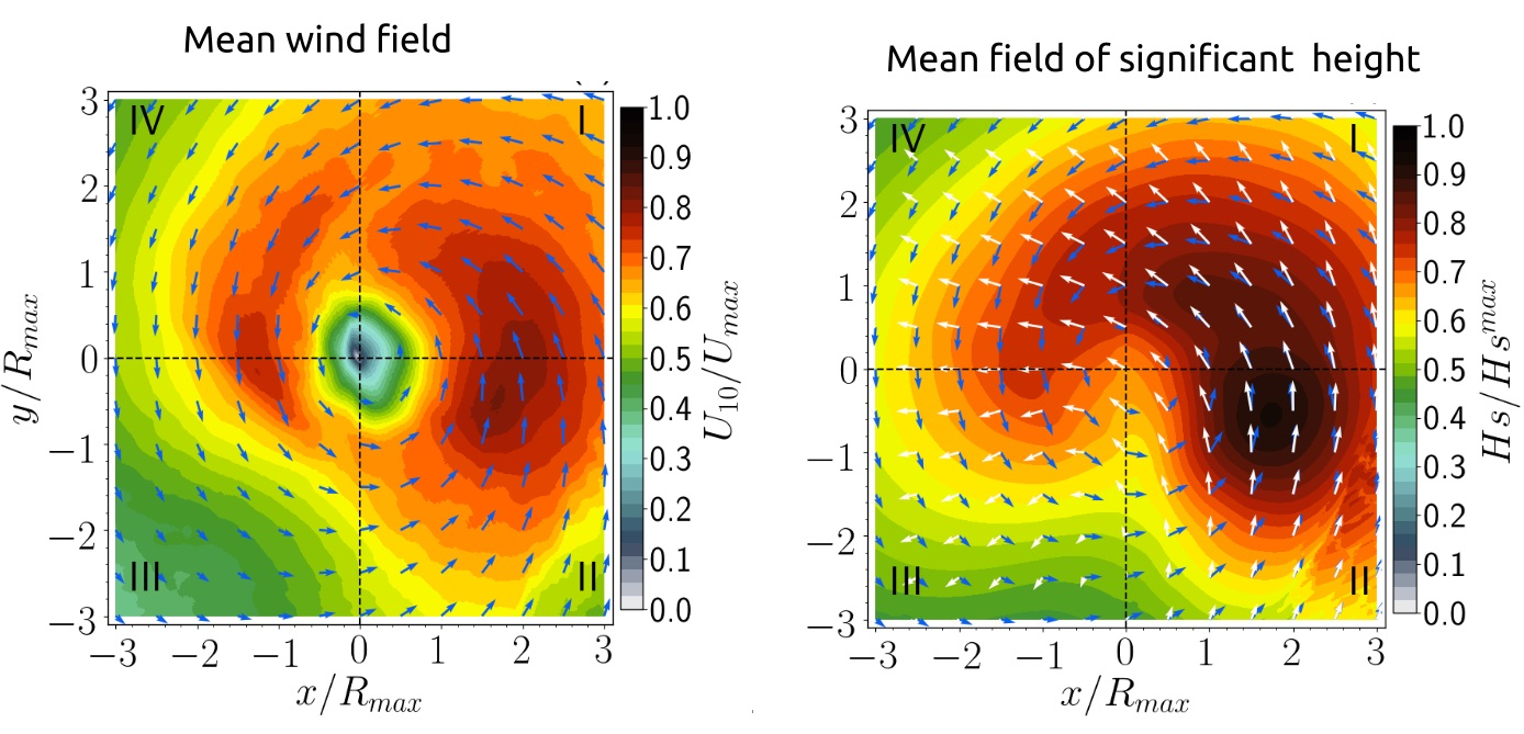
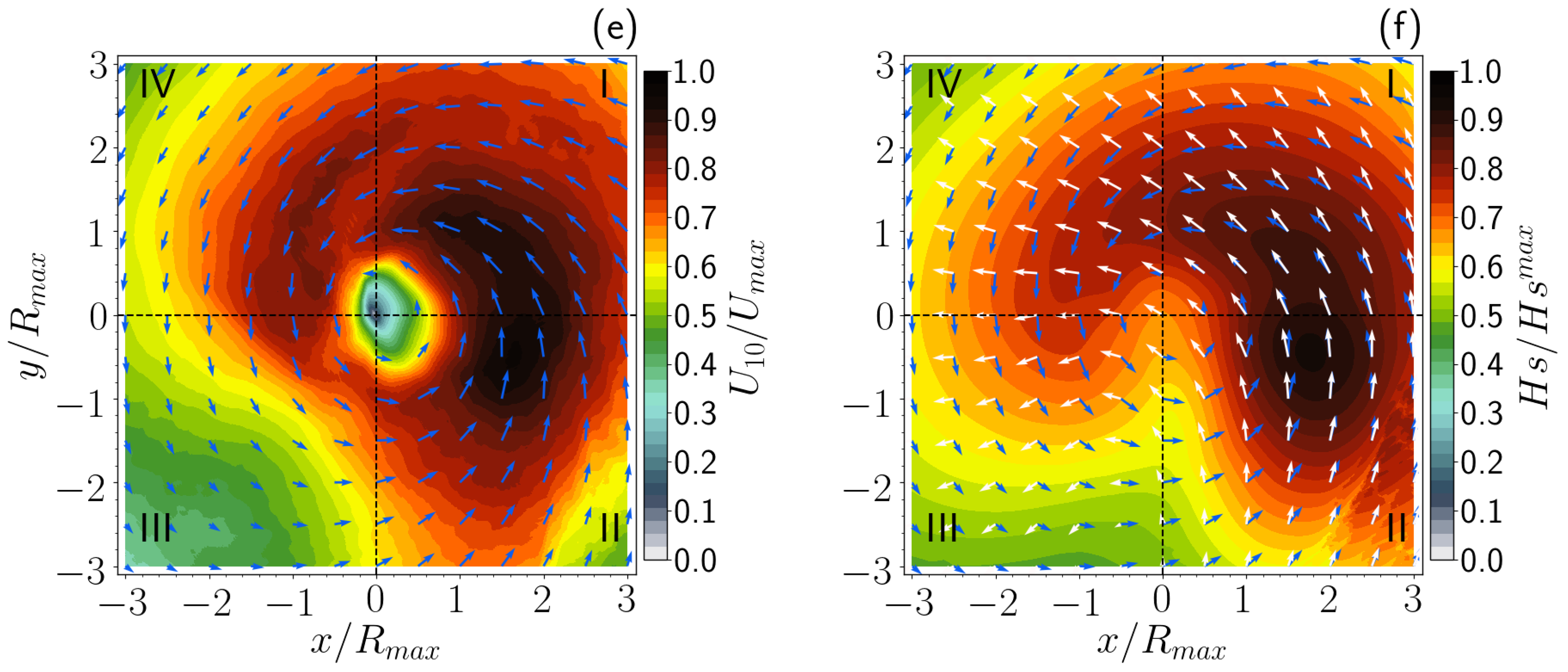
In order to assess the effect of wind variability on the wave field structure over a short period, a 3 h interval centered on the date when the storm reaches hurricane status (blue dashed line in Figure 2b) is analyzed. It is worth noting that this is a period of sudden increase in maximum wind intensity and translation speed of the TC (see Figure 2b,d). In this case, the wave fields are calculated using both the original and filtered wind fields. Figure 7a,c, shows the average wind field; whereas, Figure 7b,d shows the average fields. As in the previous examples, each field is normalized with its own maximum value.
The average wind field computed with original data (Figure 7a) shows a very different structure with respect to the one computed over a larger period (see Figure 4a). This exhibits the high time-space variability of the wind field, only visible when the TC is reproduced with enough time and space resolution. It is possible to observe the presence of intense winds both on the right and left quadrants. In fact, the maximum winds are present in quadrants III and IV, at a distance of 1. This behavior differs much with respect to the typical structure obtained from the parametric hurricanes described in the literature. The mean field (Figure 7b) shows a spatial structure similar to that computed with a larger set of data (see, e.g., Figure 4b). The higher average values are seen in the right quadrants of the TC, at distances greater than . Large values are also observed in quadrants III and IV, which are associated with the wind maxima for the same regions (Figure 7a). By contrast, using the filtered data, and average fields (Figure 7c,d, respectively) show the same patterns as those seen with the original wind data. Nonetheless, the mean fields have normalized values greater than those obtained with the unfiltered data (Figure 7a). This is due to the maximum wind values used to normalize the corresponding fields which are smaller. This behavior is not observed in the averaged fields computed with the smoothed field, because a reduced time variability of the field will induce lower values.
The comparison between average fields computed over a relatively long period against those computed over short periods indicate a high variability in the TC wind field. Although the structure of the field within the TC may show a similar behavior to the one described in Figure 7, the average field tends to be similar to that of Figure 4 if it is analyzed through a sufficiently long period. Nonetheless, the mean field shows a rather persistent spatial structure, with maximum values located mainly in the front (I and IV) and second quadrants. This behavior is associated with an extended fetch condition over the right quadrants [4,11], which implies that the waves in this sector are forced by the wind over a longer period. In this case, the storm translation speed, , plays an important role in the generation and development of , and also on the TC waves distribution [10]. For this condition to be present, must be comparable to the wave group velocity. This process allows the wind, by constantly blowing over the right side of the TC, to favor wave trapping inside the cyclone and to generate larger local waves [11].
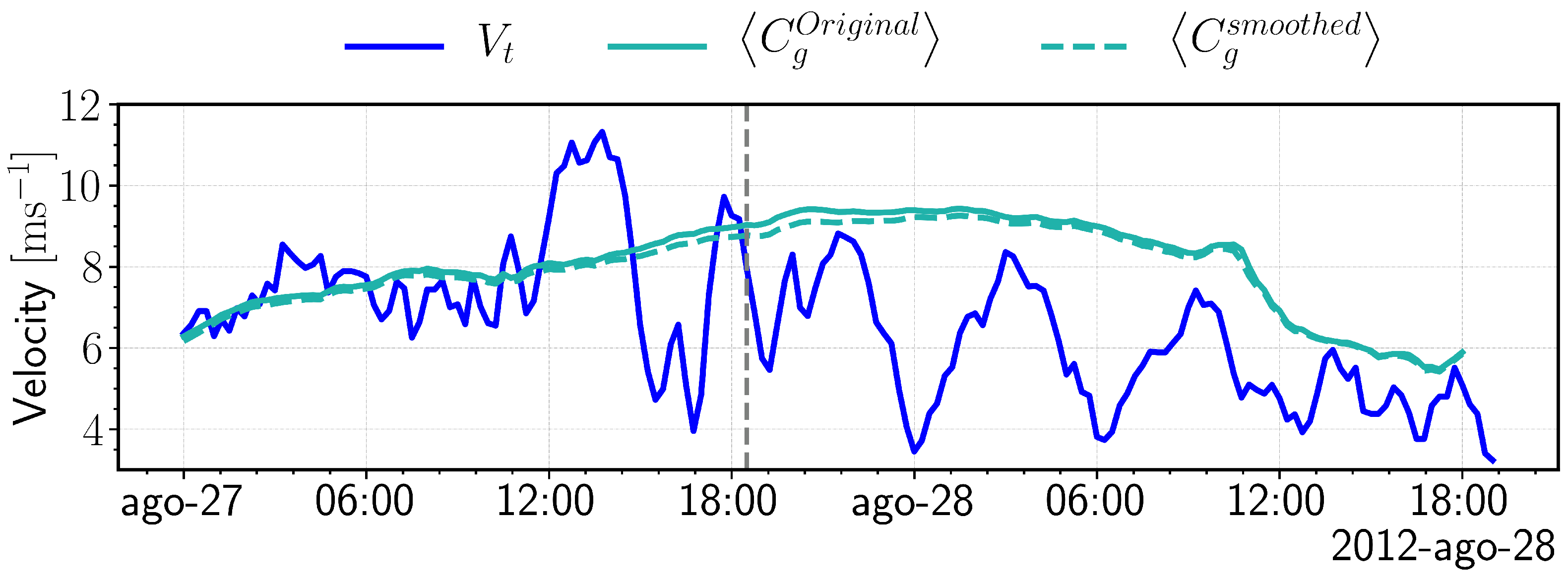
Based on the direction of the spectral peak values computed by the wave model, it is possible to obtain the waves’ average group velocity at the right quadrants of the TC (I and II), and to make a comparison with the computed using the HWRF output. These results are shown in Figure 8. On average, (7.2 ms) and (8.3 ms) are nearly equal. Particularly, during the period in which the TC reaches the hurricane category (Figure 7), large wave heights are observed covering—almost totally—quadrant I, regardless of the fact that intense winds are present in quadrants III and IV. The presence of high values in quadrant II is mostly associated with the intensity of , as well as to the extended fetch condition; whereas, the high values in the front quadrants seem to be linked to the wind intensity and to the greatest values with respect to the mean .
3.3. Temporal Variability of the Wind and Significant Wave Height Fields
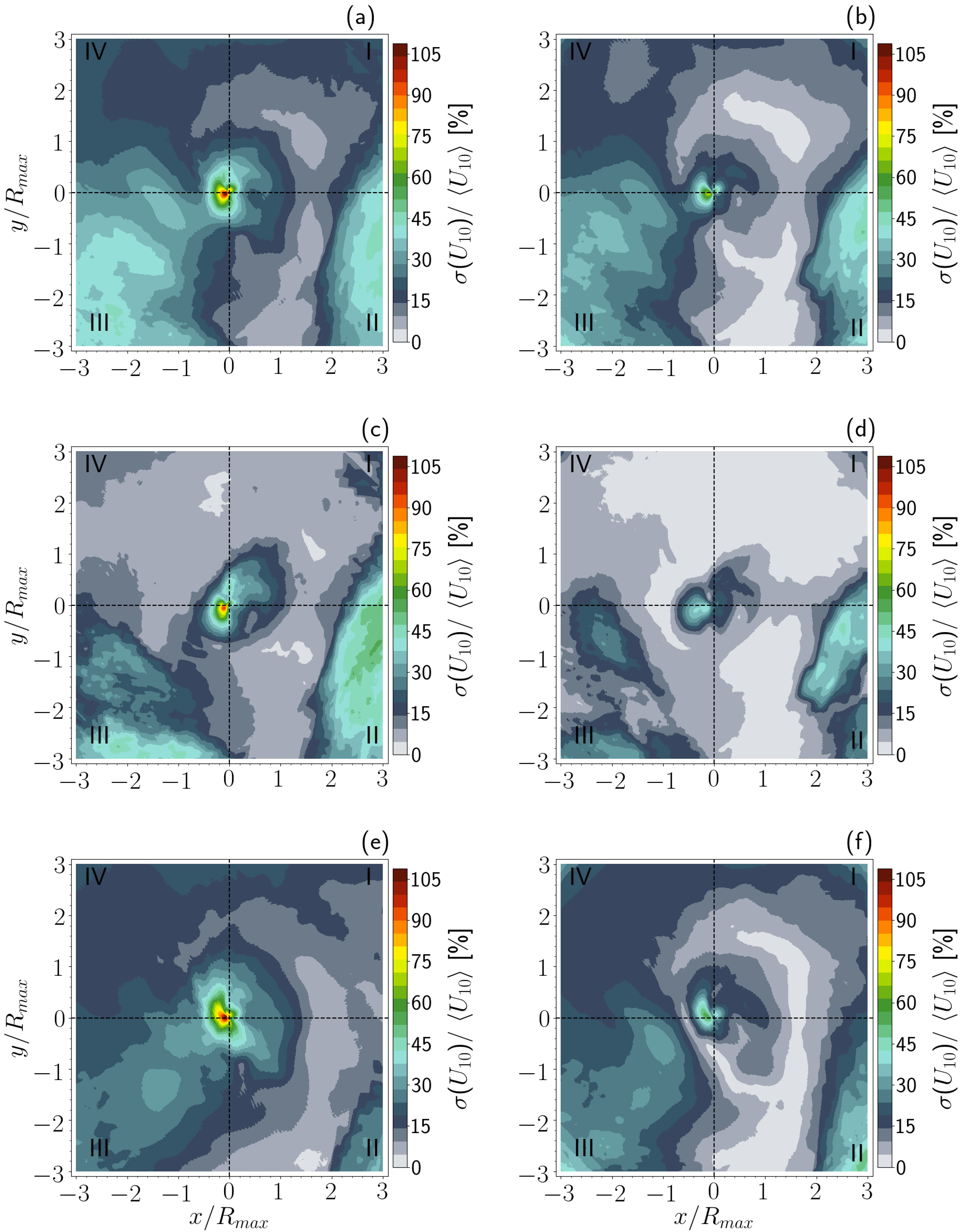
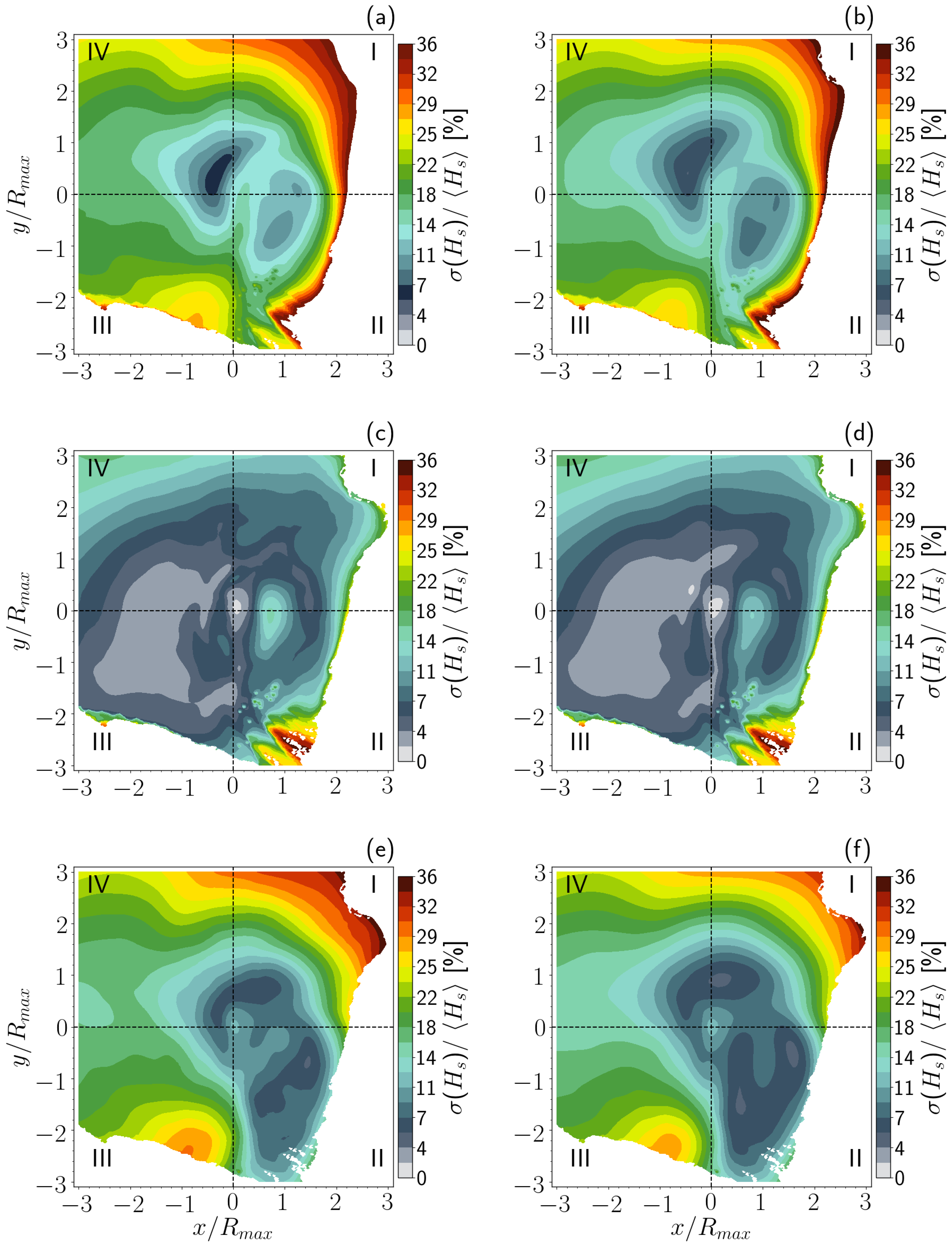
The temporal variability of the wind and significant wave height fields are determined by computing the standard deviation normalized by its respective average field. The normalization process is considered a measure of the data dispersion, which allows the determination of the variability between them, in relation to their mean value [47]. The normalized standard deviation values are expressed in percentage. Three important variability regions are present within the 18 h average wind field (Figure 9a), as well as during the moderate storm (Figure 9c) and intensification (Figure 9e) stages. The first region is associated with low variability (less than 27%) and is located in the right quadrants (I and II), at a distance of about 1, thus belonging to the zone characterized by the maximum winds. During the moderate stage, the region with a low variability values is spatially enhanced to 3 in quadrants I and IV, but the variability percentage reduces from 27% to values even lower than 7%. During the intensification stage (Figure 9e), the variability percentage rises up to 27%, thus being very close to the value obtained when a total of 18 h is considered (Figure 9a).
The second region with characteristics variability is located at quadrant III, away from the eye of the TC. Using the 18 h scheme, the variability oscillates between 21–48%; when the storm is moderate (Figure 9c), the variability reduces to 27% and, when the storm is intensified, it increases to 34%. Finally, the third variability region is around the eye of the TC. This area is defined by Weatherford and Gray [48] as the inner core of the storm, reaching to (∼111 km), and presenting the higher variability percentage.
As for the 18 h interval, the variability ranges from 41% to 109%; during the moderate stage, it is slightly reduced together with its spatial distribution and, when the storm is intensified, there is a considerable rise in the variability which reaches a maximum of 109%. At every stage of the storm, the minimum variability region is located in quadrants I and II, so this region is representative of the average features. Very low variability values at these regions is indicative of a nearly-constant wind direction. The third region characterized by high variability is also seen in the vicinity of the storm eye, which is likely to be generated by strong velocity gradients as well as rapid variations in the wind direction at the region adjacent to the cyclone’s eyewall [40].
The variability field computed with the filtered data is presented in Figure 9b,d,f. As in the unfiltered case, three main regions are distinguished but with the expected variability reduction due to the filtering process. Particularly, during the 18 h interval (Figure 9b) the minimum variability region located right of the TC eye is maintained below 14%; that value is notably reduced to almost zero during the moderate storm stage (Figure 10d), and extends up to 3 over the four quadrants of the storm. During the intensification stage (Figure 9f), the variability is slightly higher than that of the moderate storm stage, with approximately 27%. The second variability region, located at quadrant II, has percentage values similar to those computed using the unfiltered data (27–41%). As for the vicinity of the TC eye, the variability percentage was reduced, ranging from 41% to 68%.
Figure 10 shows the time variability field using the original and filtered data for the different storm stages. As in the wind fields from Figure 9, a region of minimum variability is observed to the right of the storm center during the three stages. The variability level fluctuates from 11% during the 18 h interval to 16% during the moderate storm stage, then reduces to 5% during the intensification stage. In addition, during the moderate stage, this region of low variability expands over the four quadrants of the TC, and then it is spatially reduced during the intensification stage. Unlike the wind field, the variability level does not show high percentage values around the storm eye. As seen in Figure 10e, the greatest variability is found beyond .
Figure 10b,d,f, shows the variability computed with wind filtered data. The results are similar to those obtained with the original wind data, specifically, those low-variability values in quadrants I and IV, as well as an expansion directed away from the center. Additionally, the level of variability computed using the unfiltered wind data is somewhat maintained.
When analyzing the 3 h interval in which the storm becomes a category 1 hurricane, the wind variability (Figure 11a,c) is observed to be similar as in the distinct storm stages (Figure 9a,c,e). The high variability is located around the TC center and extends to . The lower variability percentage (14%) is still present in quadrant III. The time variability of (Figure 11b,d) during this period shows values below 10% within 1, mainly over quadrant I and III. The highest variability (∼10%) is observed in quadrant II, between 2 and 3. In general, presents slight variations which become more evident when reduced time intervals are considered.
4. Discussion
Our results show that the atmospheric model HWRF has the capability to reproduce the trajectory, , and of the TC Isaac in agreement with the NHC reports. However, the values of simulated with the HWRF (Figure 2d, solid blue line) show high variability in contrast with the NHC observations. The variations of with respect to the NHC observations could be attributed to the appropriate simulation of the internal parameters of the storm, particularly of , which has been reported to have a positive correlation with [49,50]. In addition, the good estimation of the internal parameters of the TC could be a result of using the HWRF physically configured for hurricanes [20]. The latter allows the generation of high time resolution wind data, unlike the HWIND wind fields used by NHC, which have a time resolution of 3 or 6 h.
The variability of (see Figure 3c) from the model time series is larger with respect to the buoy observations, probably due to differences in the calculation of the eye size at those specific times. According to the HWRF results, the further intensification of the registered wind is faster than the observed, but the decreasing tendency is similar. The values of (Figure 3c) computed by the HWRF at the vicinity of the storm eye indicate a model tendency to overestimate its magnitude, which is consistent with the translation speed overestimation [38]. By eliminating the 3 h variability of the original wind and fields, a reduced spatial distribution of variability level was observed when compared to the original data, together with the reduction in the values. In addition, when averaging over a short time lapse (i.e., 3 h, when the storm had a hurricane category as in Figure 7), the maximum winds are reproduced in quadrants III and IV, at a distance of 1 . This behavior is importantly different with respect to the typical structure obtained from the parametric hurricanes described in the literature. The mean field shows a very persistent structure, with the maximum values located mainly in the front (I and IV) and second quadrants associated with an extended fetch condition. The comparison between the fields computed with a relatively long period, against those computed with short periods indicate a high variability in the TC wind field. Moreover, in Figure 10, the presents slight variations which become more evident when reduced time intervals are considered. The observed variability in the wind field and shows the importance of using high time resolution wind fields as forcing agents of the wind wave models, as was already suggested by Ponce and Ocampo-Torres [46], Tolman and Alves [25] as well as Collins et al. [51].
5. Conclusions
In this work, space-time variability of the wind field under tropical cyclone conditions was determined using numerical simulations of realistic wind fields with high space and time resolution. The atmospheric model HWRF was used to generate the wind fields and was configured to reproduce the evolution of hurricane Isaac during its passage through the GoM in the last few days of August 2012. Based on the realistic wind field obtained with the HWRF model, the wind wave field was computed using the third generation spectral model WaveWatch III. The main objective of this work is to determine the extent to which the high time and space variability of the wind field impacts on the evolution of the wind waves field during the development of these extreme events. The effect of the time resolution is analyzed by using the HWRF-generated data with an interval of 15 min (original data), as well as a 3 h filtered version of the same database (keeping t = 15 min). Both datasets are used to simulate the wave field. Although reproducing the exact characteristics of hurricane Isaac is not intended here, a comparative analysis of the wind and wave fields is carried out using observations and the model-generated results in order to validate the simulated output. The numerical results indicate that the structure of the wind field has a high time and space variability, although it has an overall structure very similar to those reported for parametric hurricanes, as long as the number of averaged hours is sufficiently high. If a shorter time interval is analyzed (as in a 3 h study case, in which period the storm becomes a category 1 hurricane), the structure of the mean wind field may importantly differ from the mean field computed with a sufficiently longer period.
The wind waves response shows that, although the extended fetch is present in the TC, it becomes more important during the intensification stage of the storm, since it allows a considerable wave growth to the right of the TC when the wind maximum is on the left of the TC. For this condition to be developed, the and values must be of the same order; here, reached 7.2 ms and was of 8.3 ms. This phenomena causes the waves located to the right of the storm to be trapped for a prolonged period and distance, with the presence of previously generated swell and local wind waves. While to the left of the TC the waves are local and not trapped, wave growth is also inhibited because the wind blows for a shorter period. The implications of the obtained results are the following:
- The wave field generated by the WaveWatch III model does not respond instantly to the variations in the wind field structure. More studies and specialized measurements are required to determine if the described behavior is either physically realistic, or is a deficiency of the wave model.
- The results indicate that the structure of the wave field is strongly determined by the extended fetch process, which leads to the occurrence of high waves over quadrants I and II of the storm. The high wave values over the frontal quadrant IV are related to a translation speed of the TC smaller than the group velocity of the waves generated in quadrants I and II.
- The wind field generated by parametric hurricanes successfully reproduces the wave field structure because the mean wind field has a tendency to produce a typical asymmetric spatial structure.
Author Contributions
Conceptualization, P.O., B.E.-T., N.R. and F.J.O.-T.; Methodology, N.R.; Investigation, L.P.-S.; Writing–original draft, L.P.-S.; Writing–review & editing, P.O. and F.J.O.-T.; Visualization, L.P.-S.; Supervision, P.O. All authors have read and agreed to the published version of the manuscript.
Funding
This research was funded by Centro de Investigación Científica y de Educación Superior de Ensenada (CICESE).
Institutional Review Board Statement
Not applicable.
Informed Consent Statement
Not applicable.
Data Availability Statement
Not applicable.
Acknowledgments
L.M.P.-S. wishes to express her gratitude to CONACYT and the Physical Oceanography Department of CICESE, Mexico for the support provided as a PhD scholarship. The support of Héctor García-Nava, Cuauhtémoc Turrent-Thompson, Enric Pallàs-Sanz, Paula Pérez-Brunius, Rafael Ramirez-Mendoza and Froylan Rosas-Villegas is also acknowledged. The authors are grateful to the anonymous referees for their constructive comments and suggestions.
Conflicts of Interest
The authors declare no conflict of interest.
References
- Wang, Y.; Wu, C.C. Current understanding of tropical cyclone structure and intensity changes—A review. Meteorol. Atmos. Phys. 2004, 87, 257–278. [Google Scholar] [CrossRef]
- Emanuel, K. Increasing Destructiveness of Tropical Cyclones Over the Past 30 Years. Nature 2005, 436, 686–688. [Google Scholar] [CrossRef]
- Wang, Y. Recent research progress on tropical cyclone structure and intensity. Trop. Cyclone Res. Rev. 2012, 1, 254–275. [Google Scholar] [CrossRef]
- Moon, I.J.; Ginis, I.; Hara, T.; Tolman, H.L.; Wright, C.W.; Walsh, E.J. Numerical Simulation of Sea Surface Directional Wave Spectra under Hurricane Wind Forcing. J. Phys. Oceanogr. 2003, 33, 1680–1706. [Google Scholar] [CrossRef] [Green Version]
- Chen, S.S.; Curcic, M. Ocean surface waves in Hurricane Ike (2008) and Superstorm Sandy (2012): Coupled model predictions and observations. Ocean Model. 2016, 103, 161–176. [Google Scholar] [CrossRef] [Green Version]
- Wright, C.W.; Walsh, E.; Vandemark, D.; Krabill, W.; Garcia, A.; Houston, S.; Powell, M.; Black, P.; Marks, F. Hurricane directional wave spectrum spatial variation in the open ocean. J. Phys. Oceanogr. 2001, 31, 2472–2488. [Google Scholar] [CrossRef]
- Kumar, B.P.; Stone, G.W. Numerical simulation of typhoon wind forcing in the Korean seas using a spectral wave model. J. Coast. Res. 2007, 23, 362–373. [Google Scholar] [CrossRef]
- Holthuijsen, L.; Powell, M.; Pietrzak, J. Wind and waves in extreme hurricanes. J. Geophys. Res. Ocean. 2012, 117, 9003. [Google Scholar] [CrossRef] [Green Version]
- Esquivel-Trava, B.; Ocampo Torres, F.; Osuna, P. Spatial structure of directional wave spectra in hurricanes. Ocean Dyn. 2015, 65, 65–76. [Google Scholar] [CrossRef]
- Tamizi, A.; Young, I. The Spatial Distribution of Ocean Waves in Tropical Cyclones. J. Phys. Oceanogr. 2020, 50, 2123–2139. [Google Scholar] [CrossRef]
- Liu, H.; Xie, L.; Pietrafesa, L.; Bao, S. Sensitivity of wind waves to hurricane wind characteristics. Ocean Model. 2007, 18, 37–52. [Google Scholar] [CrossRef]
- Montoya, R.; Osorio Arias, A.; Ortiz Royero, J.; Ocampo-Torres, F. A wave parameters and directional spectrum analysis for extreme winds. Ocean Eng. 2013, 67, 100–118. [Google Scholar] [CrossRef]
- Ruiz Salcines, P.; Salles, P.; Robles-Diaz, L.; Díaz-Hernández, G.; Torres-Freyermuth, A.; Appendini, C. On the Use of Parametric Wind Models for Wind Wave Modeling under Tropical Cyclones. Water 2019, 11, 2044. [Google Scholar] [CrossRef] [Green Version]
- Young, I. Directional spectra of hurricane wind waves. J. Geophys. Res. Ocean. 2006, 111, 14. [Google Scholar] [CrossRef]
- Fan, Y.; Ginis, I.; Hara, T.; Wright, C.W.; Walsh, E.J. Numerical Simulations and Observations of Surface Wave Fields under an Extreme Tropical Cyclone. J. Phys. Oceanogr. 2009, 39, 2097–2116. [Google Scholar] [CrossRef]
- Wang, D.; Kukulka, T.; Reichl, B.G.; Hara, T.; Ginis, I. Wind–Wave Misalignment Effects on Langmuir Turbulence in Tropical Cyclone Conditions. J. Phys. Oceanogr. 2019, 49, 3109–3126. [Google Scholar] [CrossRef]
- Chao, Y.; Alves, J.; Tolman, H. An Operational System for Predicting Hurricane-Generated Wind Waves in the North Atlantic Ocean. Weather. Forecast. 2005, 20, 652–671. [Google Scholar] [CrossRef] [Green Version]
- Powell, M.D.; Houston, S.H.; Amat, L.R.; Morisseau-Leroy, N. The HRD real-time hurricane wind analysis system. J. Wind. Eng. Ind. Aerodyn. 1998, 77, 53–64. [Google Scholar] [CrossRef]
- Holland, G.J. An analytic model of the wind and pressure profiles in hurricanes. Natl. Emerg. Train. Center. 1980, 108, 7. [Google Scholar] [CrossRef]
- Dodla, V.B.; Desamsetti, S.; Yerramilli, A. A comparison of HWRF, ARW and NMM models in Hurricane Katrina (2005) simulation. Int. J. Environ. Res. Public Health 2011, 8, 2447–2469. [Google Scholar] [CrossRef] [Green Version]
- Grell, G.A.; Dudhia, J.; Stauffer, D.R. A Description of the Fifth-Generation Penn State/NCAR Mesoscale Model (MM5); NCAR Technical Note; University Corporation for Atmospheric Research: Boulder, CO, USA, 1994. [Google Scholar]
- Dudhia, J. A nonhydrostatic version of the Penn State–NCAR mesoscale model: Validation tests and simulation of an Atlantic cyclone and cold front. Mon. Weather Rev. 1993, 121, 1493–1513. [Google Scholar] [CrossRef]
- Tenerelli, J.; Chen, S. High-resolution simulations of Hurricane Floyd using MM5 with vortex-following mesh refinement. In Proceedings of the Conference on Weather Analysis and Forecasting, Santiago de Compostela, Spain, 15–18 July 2001; Volume 18, pp. J52–J54. [Google Scholar]
- Pérez-Alarcón, A.; Díaz-Rodríguez, O.; Fernández-Alvarez, J.C.; Pérez-Suárez, R.; Coll-Hidalgo, P. A Comparison between the Atmospheric Component of HWRF System and WRF-HWRF Model Using Different Horizontal Resolutions in Hurricane Irma (2017) Simulation. Part I. Rev. Bras. Meteorol. 2021, 36, 183–196. [Google Scholar] [CrossRef]
- Tolman, H.L.; Alves, J.H.G. Numerical modeling of wind waves generated by tropical cyclones using moving grids. Ocean Model. 2005, 9, 305–323. [Google Scholar] [CrossRef]
- Pianezze, J.; Barthe, C.; Bielli, S.; Tulet, P.; Jullien, S.; Cambon, G.; Bousquet, O.; Claeys, M.; Cordier, E. A new coupl;ed ocean-waves-atmosphere model designed for tropical storm studies: Example of tropical cyclone Bejisa (2013–2014) in the Southe-West Indian Ocean. J. Adv. Model. Earth Syst. 2018, 10, 801–825. [Google Scholar] [CrossRef]
- Biswas, M.K.; Bernardet, L.; Ginis, I.; Kwon, Y.; Liu, B.; Liu, Q.; Marchok, T.; Mehra, A.; Newman, K.; Sheinin, D.; et al. Hurricane Weather Research and Forecasting (HWRF) Model: 2016 Scientific Documentation; University Corporation for Atmospheric Research: Boulder, CO, USA, 2016. [Google Scholar]
- Gopalakrishnan, S.; Liu, Q.; Marchok, T.; Sheinin, D.; Surgi, N.; Tuleya, R.; Yablonsky, R.; Zhang, X. Hurricane Weather Research and Forecasting (HWRF) model scientific documentation. Dev. Testbed Cent. 2010, 75, 7655. [Google Scholar]
- Powell, M.; Vickery, P.; Reinhold, T. Reduced drag coefficient for high wind speeds in tropical cyclones. Nature 2003, 422, 279–283. [Google Scholar] [CrossRef]
- Arakawa, A.; Schubert, W.H. Interaction of a Cumulus Cloud Ensemble with the Large-Scale Environment, Part I. J. Atmos. Sci. 1974, 31, 674–701. [Google Scholar] [CrossRef]
- Grell, G.A. Prognostic Evaluation of Assumptions Used by Cumulus Parameterizations. Mon. Weather. Rev. 1993, 121, 764–787. [Google Scholar] [CrossRef]
- Ferrier, B. An efficient mixed-phase cloud and precipitation scheme for use in operational NWP models. AGU Spring Meet. Abstr. 2005, 2005, A42A-02. [Google Scholar]
- WW3DG. User Manual and System Documentation of WAVEWATCH III® Version 6.07; Tech. Note 333; NOAA/NWS/NCEP/MMAB: College Park, MD, USA, 2019; 465p. [Google Scholar]
- Donelan, M.A.; Babanin, A.V.; Young, I.R.; Banner, M.L. Wave-Follower Field Measurements of the Wind-Input Spectral Function. Part II: Parameterization of the Wind Input. J. Phys. Oceanogr. 2006, 36, 1672–1689. [Google Scholar] [CrossRef]
- Rogers, W.E.; Babanin, A.V.; Wang, D.W. Observation-consistent input and whitecapping dissipation in a model for wind-generated surface waves: Description and simple calculations. J. Atmos. Ocean. Technol. 2012, 29, 1329–1346. [Google Scholar] [CrossRef]
- Zieger, S.; Babanin, A.V.; Rogers, W.E.; Young, I.R. Observation-based source terms in the third-generation wave model WAVEWATCH. Ocean Model. 2015, 96, 2–25. [Google Scholar] [CrossRef] [Green Version]
- Curcic, M.; Chen, S.S.; Özgökmen, T. Hurricane–induced ocean waves and stokes drift and their impact on surface transport and dispersion in the Gulf of Mexico. Geophys. Res. Lett. 2016, 43, 2773–2781. [Google Scholar] [CrossRef]
- Inagaki, N.; Shibayama, T.; Esteban, M.; Takabatake, T. Effect of translate speed of typhoon on wind waves. Nat. Hazards 2021, 105, 841–858. [Google Scholar] [CrossRef]
- Janssen, P. Nonlinear Wave–Wave Interactions and Wave Dissipation; Cambridge University Press: Cambridge, UK, 2004; pp. 129–208. [Google Scholar] [CrossRef]
- Zhao, W.; Guan, S.; Hong, X.; Li, P.; Tian, J. Examination of wind-wave interaction source term in WAVEWATCH III with tropical cyclone wind forcing. Acta Oceanol. Sin. 2011, 30, 1–13. [Google Scholar] [CrossRef]
- Tolman, H.L.; Alves, J.H.G.; Chao, Y.Y. Operational forecasting of wind-generated waves by Hurricane Isabel at NCEP. Weather. Forecast. 2005, 20, 544–557. [Google Scholar] [CrossRef] [Green Version]
- Zhuo, L.; Wang, A.; Guo, P. Numerical simulation of sea surface directional wave spectra under typhoon wind forcing Export. J. Hydrodyn. Ser. B 2008, 20, 776–783. [Google Scholar] [CrossRef]
- Hu, K.; Chen, Q. Directional spectra of hurricane-generated waves in the Gulf of Mexico. Geophys. Res. Lett. 2011, 38, 1–7. [Google Scholar] [CrossRef]
- Mora Escalante, R.E. Estudio Numérico Sobre la Estructura del Campo de olas en Condiciones de Huracán. Master’s Thesis, Centro de Investigación Científica y de Educación Superior de Ensenada, Baja California, Ensenada, Mexico, 2015. [Google Scholar]
- Hwang, P.A.; Fan, Y.; Ocampo-Torres, F.J.; García-Nava, H. Ocean surface wave spectra inside tropical cyclones. J. Phys. Oceanogr. 2017, 47, 2393–2417. [Google Scholar] [CrossRef]
- Ponce, S.; Ocampo-Torres, F.J. Sensitivity of a wave model to wind variability. J. Geophys. Res. Ocean. 1998, 103, 3179–3201. [Google Scholar] [CrossRef] [Green Version]
- Glover, D.M.; Jenkins, W.J.; Doney, S.C. Modeling Methods for Marine Science; Cambridge University Press: Cambridge, UK, 2011. [Google Scholar] [CrossRef]
- Weatherford, C.L.; Gray, W.M. Typhoon structure as revealed by aircraft reconnaissance. Part I: Data analysis and climatology. Mon. Weather Rev. 1988, 116, 1032–1043. [Google Scholar] [CrossRef]
- Mei, W.; Pasquero, C.; Primeau, F. The effect of translation speed upon the intensity of tropical cyclones over the tropical ocean. Geophys. Res. Lett. 2012, 39, 1–6. [Google Scholar] [CrossRef] [Green Version]
- Kossin, J.P.; Emanuel, K.A.; Vecchi, G.A. The poleward migration of the location of tropical cyclone maximum intensity. Nature 2014, 509, 349–352. [Google Scholar] [CrossRef] [PubMed] [Green Version]
- Collins, C.; Hesser, T.; Rogowski, P.; Merrifield, S. Altimeter Observations of Tropical Cyclone-generated Sea States: Spatial Analysis and Operational Hindcast Evaluation. J. Mar. Sci. Eng. 2021, 9, 216. [Google Scholar] [CrossRef]
Figure 1.
Spatial domains of the HWRF atmospheric model. The area covered by the pressure field indicates the extent of the fixed domain (D01), the black segmented line indicates the area covered by the second mobile domain (D02) and the red segmented line indicates the third mobile domain (D03).
Figure 1.
Spatial domains of the HWRF atmospheric model. The area covered by the pressure field indicates the extent of the fixed domain (D01), the black segmented line indicates the area covered by the second mobile domain (D02) and the red segmented line indicates the third mobile domain (D03).

Figure 2.
(a) Trajectory of hurricane Isaac reported by the NHC (solid black line) and the one obtained with the HWRF model (solid blue line). The colored dots represent the time of the simulation. The position of the NDBC buoys used here is denoted with triangle-shaped markers. (b) Time series of the maximum sustained wind at 10 m, (c) minimum pressure and (d) translation speed of the TC. The blue dashed line in (b) indicates the time at which the storm became a category 1 hurricane according to the model, whereas the date reported by the NHC is indicated with a gray dashed line. In (d), the blue dashed line represents the fitting of the values computed by the HWRF.

Figure 3.
Time evolution of and computed by HWRF and WW3 models, respectively, as well as the observations from the NDBC buoys 42001 (left panels) and 42003 (right panels).
Figure 3.
Time evolution of and computed by HWRF and WW3 models, respectively, as well as the observations from the NDBC buoys 42001 (left panels) and 42003 (right panels).

Figure 4.
Wind fields (left) and mean significant wave height (right) obtained with original data. (a) and (b) fields with an 18 h interval. Wind field (c) and significant wave height (d) for the moderate storm stage. Intensification stage for the wind field (e) and significant wave height (f).
Figure 4.
Wind fields (left) and mean significant wave height (right) obtained with original data. (a) and (b) fields with an 18 h interval. Wind field (c) and significant wave height (d) for the moderate storm stage. Intensification stage for the wind field (e) and significant wave height (f).

Figure 5.
Wind fields (left) and mean significant wave height (right) obtained with the 3 h running mean filtered data. (a) and (b) fields with an 18 h interval. Wind field (c) and significant wave height (d) for the moderate storm stage. Intensification stage for the wind field (e) and significant wave height (f).


Figure 6.
Differences (in percentage) between the 97.5 percentile values of the calculated using the original winds minus those calculated using the filtered winds.
Figure 6.
Differences (in percentage) between the 97.5 percentile values of the calculated using the original winds minus those calculated using the filtered winds.

Figure 7.
Average and fields for the 3 h period in which the storm reaches the category 1 hurricane stage. At the top panel, the wind (a) and significant wave height (b) average fields computed with the original data. At the lower panel, the wind (c) and significant wave height (d) average fields are computed with filtered data.

Figure 8.
Evolution of the TC translation speed, and the wave’s average group velocity () using the original (light-blue solid line) and filtered results (light-blue dashed line).
Figure 8.
Evolution of the TC translation speed, and the wave’s average group velocity () using the original (light-blue solid line) and filtered results (light-blue dashed line).

Figure 9.
Temporal variability of the wind field computed with the original (left) and filtered (right) data. The panel levels represent the 18 h scheme (top), moderate storm (center) and intensification (bottom) stages. (a) and (b) show the average for the total period (18 h); (c) and (d) show the period of moderate storm (9 h), and (e) and (f) show the intensification period (9 h).

Figure 10.
Temporal variability of the field computed with the original (left) and filtered (right) data. The panel levels represent the 18 h scheme (top), moderate storm (center) and intensification (bottom) stages. (a) and (b) show the average for the total period (18 h); (c) and (d) show the period of moderate storm (9 h), and (e) and (f) show the intensification period (9 h).

Figure 11.
Average temporal variability fields of (left) and (right) computed for the 3 h interval in which the storm becomes a category 1 hurricane. The top and bottom panels represent the results from the original (a) and (b) and filtered data (c) and (d), respectively.
Figure 11.
Average temporal variability fields of (left) and (right) computed for the 3 h interval in which the storm becomes a category 1 hurricane. The top and bottom panels represent the results from the original (a) and (b) and filtered data (c) and (d), respectively.


Table 1.
Characteristics of the grids used for the HWRF model configuration. The fixed grid is centered in the initial position of the tropical cyclone, whereas the mobile grids are centered in the instant position of the tropical cyclone eye.
Table 1.
Characteristics of the grids used for the HWRF model configuration. The fixed grid is centered in the initial position of the tropical cyclone, whereas the mobile grids are centered in the instant position of the tropical cyclone eye.
| Domain | Resolution | Grid |
|---|---|---|
| D01 | 80 × 80 (18 km) | Fixed |
| D02 | 25 × 25 (6 km) | Mobile |
| D03 | 8.3 × 8.3 (2 km) | Mobile |
Table 2.
Parameterizations used in the implementation of HWRF version 3.8.
| Physical | Parameterization |
|---|---|
| Governing Equations | Primitive equations with non-hydrostatic option (NMM) |
| Surface boundary layer | Geophysical Fluid Dynamics Laboratory (GFDL) [29] |
| Cumulus parameterization | Simplified Arakawa–Schubert (SAS) [30,31] |
| Microphysics | Ferrier–Aligo [32] |
| Vortex tracking | Geophysical Fluid Dynamics Laboratory vortex tracker |
| Vertical resolution | 61 vertical levels |
Table 3.
Physical processes parameterizations and some resolution characteristics used in the implementation of the atmospheric model WW3 version 6.07 (ST6 according to the model nomenclature).
Table 3.
Physical processes parameterizations and some resolution characteristics used in the implementation of the atmospheric model WW3 version 6.07 (ST6 according to the model nomenclature).
| Physical | Parameterization |
|---|---|
| Wind input | Donelan et al. [34] |
| Non-linear interactions | Discrete Interaction Approximation (DIA) |
| Whitecapping | Rogers et al. [35], Zieger et al. [36] |
| Microphysics | Ferrier–Aligo Ferrier [32] |
| Resolution | |
| Temporal resolution | 15 min |
| Spatial resolution | 0.02 |
| Number of frequencies | 32 (0.0373–0.7159 Hz; ) |
| Number of directions | 30 ( = 12) |
| Maximum global time step | 180 s |
| Maximum CFL time step for x-y | 60 s |
| Maximum CFL time step for k-theta | 60 s |
| Minimum source term time step | 15 s |
Table 4.
Statistical validation for the wind intensity, , and the significant wave height, , computed by the models at the corresponding positions of the NDBC buoys 42001 and 42003.
Table 4.
Statistical validation for the wind intensity, , and the significant wave height, , computed by the models at the corresponding positions of the NDBC buoys 42001 and 42003.
| Buoy | Variable | S | ||
|---|---|---|---|---|
| 42001 | [ms] | 0.75 | 0.98 | −0.22 |
| [m] | 0.85 | 0.5 | 0.32 | |
| 42003 | [ms] | 0.2 | 5.4 | 3.2 |
| [m] | 0.47 | 1.7 | 1.5 |
Disclaimer/Publisher’s Note: The statements, opinions and data contained in all publications are solely those of the individual author(s) and contributor(s) and not of MDPI and/or the editor(s). MDPI and/or the editor(s) disclaim responsibility for any injury to people or property resulting from any ideas, methods, instructions or products referred to in the content. |
© 2023 by the authors. Licensee MDPI, Basel, Switzerland. This article is an open access article distributed under the terms and conditions of the Creative Commons Attribution (CC BY) license (https://creativecommons.org/licenses/by/4.0/).
Share and Cite
MDPI and ACS Style
Pérez-Sampablo, L.; Osuna, P.; Esquivel-Trava, B.; Rascle, N.; Ocampo-Torres, F.J. Sensitivity of the Wave Field to High Time-Space Resolution Winds during a Tropical Cyclone. Oceans 2023, 4, 92-113. https://doi.org/10.3390/oceans4010008
AMA Style
Pérez-Sampablo L, Osuna P, Esquivel-Trava B, Rascle N, Ocampo-Torres FJ. Sensitivity of the Wave Field to High Time-Space Resolution Winds during a Tropical Cyclone. Oceans. 2023; 4(1):92-113. https://doi.org/10.3390/oceans4010008
Chicago/Turabian StylePérez-Sampablo, Laura, Pedro Osuna, Bernardo Esquivel-Trava, Nicolas Rascle, and Francisco J. Ocampo-Torres. 2023. "Sensitivity of the Wave Field to High Time-Space Resolution Winds during a Tropical Cyclone" Oceans 4, no. 1: 92-113. https://doi.org/10.3390/oceans4010008