
Spatiotemporal Variation in Environmental Key Parameters within Fleshy Red Algae Mats in the Mediterranean Sea

 ,
,  ,
,
Abstract
:1. Introduction
2. Materials and Methods
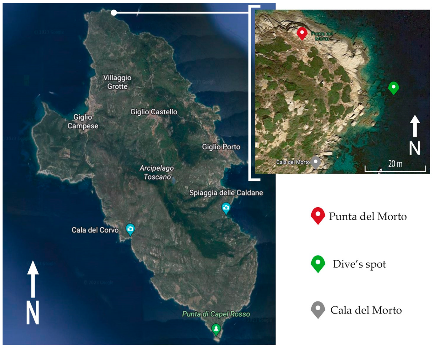
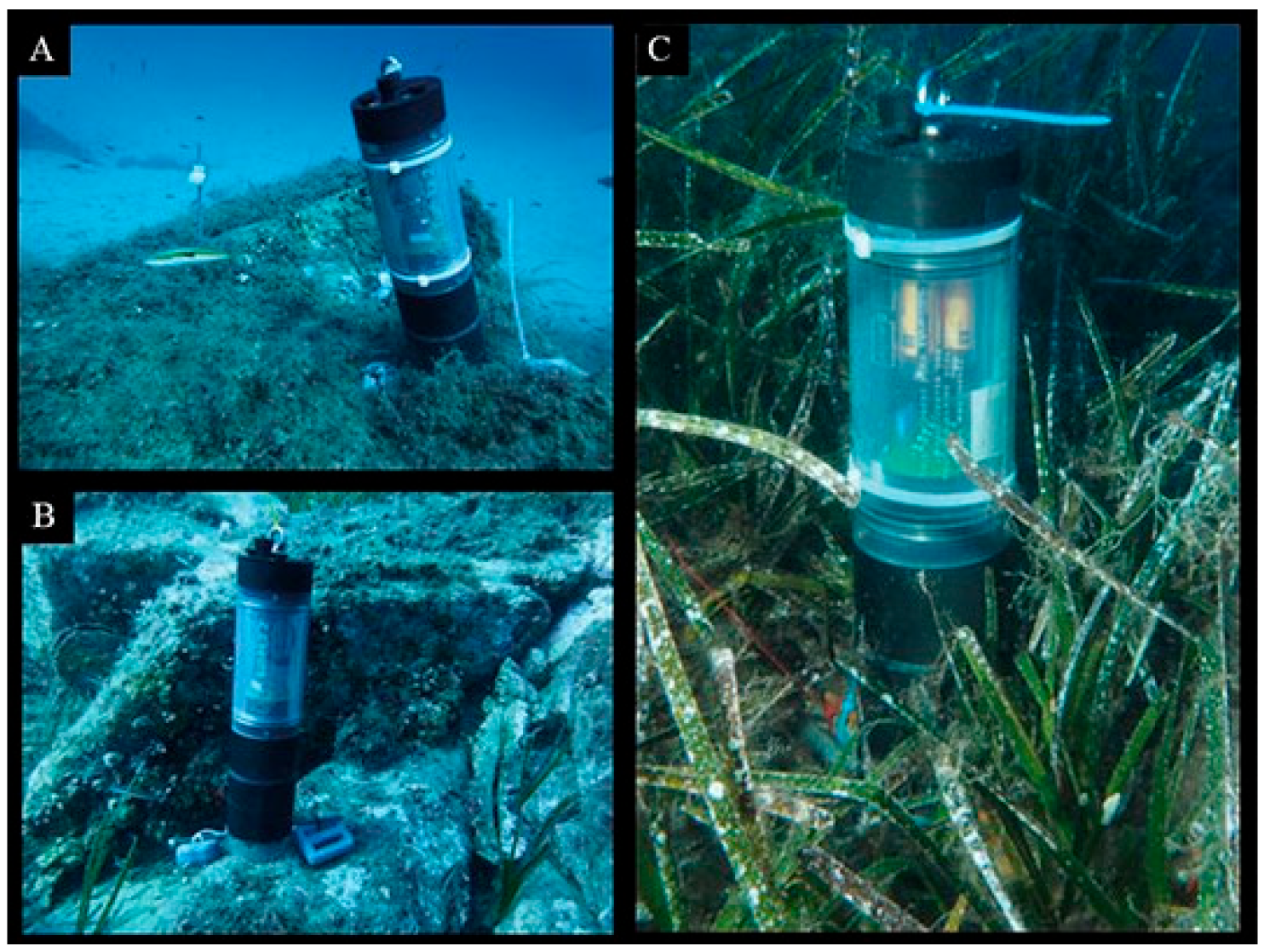
2.1. Study Area and Experimental Design
2.2. Statistical Analysis
3. Results
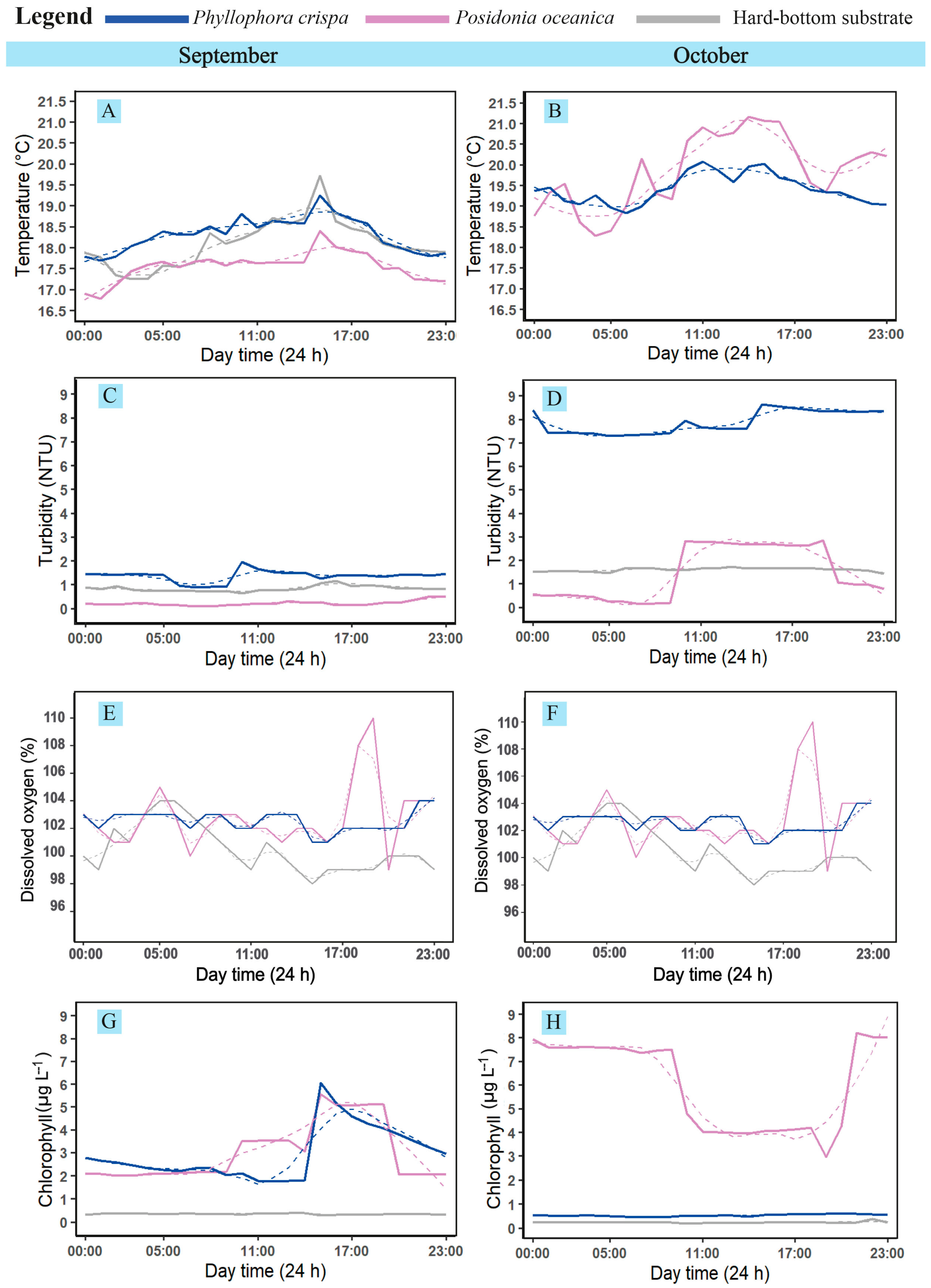
3.1. Temperature
3.2. Turbidity
3.3. Dissolved Oxygen
3.4. Chlorophyll
4. Discussion
4.1. How Do P. crispa Mats Influence Oxygen and Chlorophyll along with Turbidity and Temperature in Comparison to Neighboring Habitats?
4.2. What Is the Daily and Monthly Variation in These Key Parameters in P. crispa Mats in Comparison to Neighboring Habitats?
4.3. Ecological Implications
4.4. Limitations and Conclusions
Supplementary Materials
Author Contributions
Funding
Institutional Review Board Statement
Informed Consent Statement
Data Availability Statement
Acknowledgments
Conflicts of Interest
References
- Jones, C.G.; Lawton, J.H.; Shachak, M. Positive and Negative Effects of Organisms as Physical Ecosystem Engineers. Ecology 1997, 78, 1946–1957. [Google Scholar] [CrossRef]
- Hastings, A.; Byers, J.; Crooks, J.A.; Cuddington, K.; Jones, C.; Lambrinos, J.G.; Talley, T.S.; Wilson, W.G. Ecosystem engineering in space and time. Ecol. Lett. 2007, 10, 153–164. [Google Scholar] [CrossRef] [PubMed]
- Koch, E.W. Beyond Light: Physical, Geological, and Geochemical Parameters as Possible Submersed Aquatic Vegetation Habitat Requirements. Estuaries 2001, 24, 1–17. [Google Scholar] [CrossRef]
- Koch, E.W.; Sanford, L.P.; Chen, S.-N.; Shafer, D.J.; Smith, J.M. Waves in Seagrass Systems: Review and Technical Recommendations; Defense Technical Information Center: Fort Belvoir, VA, USA, 2006. [Google Scholar] [CrossRef]
- Via, J.D.; Sturmbauer, C.; Schönweger, G.; Sötz, E.; Mathekowitsch, S.; Stifter, M.; Rieger, R. Light gradients and meadow structure in Posidonia oceanica: Ecomorphological and functional correlates. Mar. Ecol. Prog. Ser. 1998, 163, 267–278. [Google Scholar] [CrossRef]
- Schmidt, N.; El-Khaled, Y.C.; Roßbach, F.I.; Wild, C. Fleshy Red Algae Mats Influence Their Environment in the Mediterranean Sea. Front. Mar. Sci. 2021, 8, 721626. [Google Scholar] [CrossRef]
- Arumugam, R.; Kannan, R.R.R.; Saravanan, K.R.; Thangaradjou, T.; Anantharaman, P. Hydrographic and sediment characteristics of seagrass meadows of the Gulf of Mannar Marine Biosphere Reserve, South India. Environ. Monit. Assess. 2013, 185, 8411–8427. [Google Scholar] [CrossRef]
- Bonifazi, A.; Ventura, D.; Gravina, M.F.; Lasinio, G.J.; Belluscio, A.; Ardizzone, G.D. Unusual algal turfs associated with the rhodophyta Phyllophora crispa: Benthic assemblages along a depth gradient in the Central Mediterranean Sea. Estuar. Coast. Shelf Sci. 2017, 185, 77–93. [Google Scholar] [CrossRef]
- Rossbach, F.; Casoli, E.; Beck, M.; Wild, C. Mediterranean Red Macro Algae Mats as Habitat for High Abundances of Serpulid Polychaetes. Diversity 2021, 13, 265. [Google Scholar] [CrossRef]
- Rossbach, F.I.; Casoli, E.; Plewka, J.; Schmidt, N.; Wild, C. New Insights into a Mediterranean Sea Benthic Habitat: High Diversity of Epiphytic Bryozoan Assemblages on Phyllophora crispa (Rhodophyta) Mats. Diversity 2022, 14, 346. [Google Scholar] [CrossRef]
- El-Khaled, Y.C.; Daraghmeh, N.; Tilstra, A.; Roth, F.; Huettel, M.; Rossbach, F.I.; Casoli, E.; Koester, A.; Beck, M.; Meyer, R.; et al. Fleshy red algae mats act as temporary reservoirs for sessile invertebrate biodiversity. Commun. Biol. 2022, 5, 579. [Google Scholar] [CrossRef]
- An Introduction to the Black Sea Ecology. Available online: https://aquadocs.org/bitstream/handle/1834/12945/An%20introduction%20to%20the%20Black%20sea%20ecology.pdf?sequence=1&isAllowed=y (accessed on 21 October 2022).
- Berov, D.; Todorova, V.; Dimitrov, L.; Rinde, E.; Karamfilov, V. Distribution and abundance of phytobenthic communities: Implications for connectivity and ecosystem functioning in a Black Sea Marine Protected Area. Estuar. Coast. Shelf Sci. 2018, 200, 234–247. [Google Scholar] [CrossRef]
- Zaitsev, Y. Introduction to the Black Sea Ecology; Smil Edition and Publishing Agency Ltd.: Chelmsford, UK, 2008; Available online: https://aquadocs.org/handle/1834/12945 (accessed on 21 October 2022).
- Guiry, M.D. Macroalgae of Rhodophycota, Phaeophycota, Chlorophycota, and two genera of Xanthophycota. Collect. Patrim. Nat. 2001, 50, 20–38. Available online: https://www.vliz.be/nl/personen-opzoeken?module=ref&refid=61168 (accessed on 21 October 2022).
- Navone, A.; Bianchi, C.N.; Orru, P.; Ulzega, A. Saggio di cartografia geomorfologica e bionomica nel parco marino di Tavolara-Capo coda cavallo (Sardegna Nord-Orientale). Oebalia 1992, 17, 469–478. [Google Scholar]
- El-Khaled, Y.C.; Tilstra, A.; Mezger, S.D.; Wild, C. Red and brown algae mats overgrow classical marine biodiversity hotspots in the Mediterranean Sea. Bull. Mar. Sci. 2022. [Google Scholar] [CrossRef]
- Kannel, P.R.; Lee, S.; Lee, Y.-S.; Kanel, S.R.; Khan, S.P. Application of Water Quality Indices and Dissolved Oxygen as Indicators for River Water Classification and Urban Impact Assessment. Environ. Monit. Assess. 2007, 132, 93–110. [Google Scholar] [CrossRef]
- Cicero, A.; Giovanardi, F. Classificazione dello Stato Ecologico dei Corpi Idrici delle Acque Marino Costiere; Implementazione della Direttiva IMP 2000/60/CE (ISPRA); ISPRA: Roma, Italy, 2012. [Google Scholar]
- Che Tempo Faceva a Isola del Giglio a Settembre 2019-Archivio Meteo Isola del Giglio iLMeteo. It. Available online: https://www.ilmeteo.it/portale/archivio-meteo/Isola%20del%20Giglio/2019/Settembre (accessed on 21 October 2022).
- Ross, A.; Willson, V.L. One-Way Anova. In Basic and Advanced Statistical Tests; Sense Publishers: Rotterdam, The Netherlands, 2017. [Google Scholar] [CrossRef]
- Ury, H.K.; Wiggins, A.D. Use of the Bonferroni inequality for multiple comparisons among means with post hoc contrasts. Br. J. Math. Stat. Psychol. 1974, 27, 176–178. [Google Scholar] [CrossRef]
- Wolf, M.; Sfriso, A.; Moro, I. Thermal pollution and settlement of new tropical alien species: The case of Grateloupia yinggehaiensis (Rhodophyta) in the Venice Lagoon. Estuar. Coast. Shelf Sci. 2014, 147, 11–16. [Google Scholar] [CrossRef]
- Pivato, M.; Carniello, L.; Gardner, J.; Silvestri, S.; Marani, M. Water and sediment temperature dynamics in shallow tidal environments: The role of the heat flux at the sediment-water interface. Adv. Water Resour. 2018, 113, 126–140. [Google Scholar] [CrossRef]
- Murray, L.; Wetzel, R. Oxygen production and consumption associated with the major autotrophic components in two temperate seagrass communities. Mar. Ecol. Prog. Ser. 1987, 38, 231–239. [Google Scholar] [CrossRef]
- Guerra, D. Uso di Parametri Chimico-Fisici Come Traccianti per Caratterizzare Masse d’acqua in Mediterraneo Occidentale. Misure di Ossigeno Disciolto e Salinità per la Calibrazione dei Sensori. 2017. Available online: http://dspace.unive.it/handle/10579/11881 (accessed on 21 October 2022).
- Kirk, J.T.O. Effects of suspensoids (turbidity) on penetration of solar radiation in aquatic ecosystems. Hydrobiologia 1985, 125, 195–208. [Google Scholar] [CrossRef]
- Duarte, C.M. Seagrass depth limits. Aquat. Bot. 1991, 40, 363–377. [Google Scholar] [CrossRef]
- Meyer, B.S.; Heritage, A.C. Effect of Turbidity and Depth of Immersion on Apparent Photosynthesis in Ceratophyllum Demersum. Ecology 1941, 22, 17–22. [Google Scholar] [CrossRef]
- Koch, E.W. Sediment resuspension in a shallow Thalassia testudinum banks ex König bed. Aquat. Bot. 1999, 65, 269–280. [Google Scholar] [CrossRef]
- Infantes, E.; Terrados, J.; Orfila, A.; Cañellas, B.; Álvarez-Ellacuria, A. Wave energy and the upper depth limit distribution of Posidonia oceanica. Bot. Mar. 2009, 52, 419–427. [Google Scholar] [CrossRef] [Green Version]
- Pergent, G.; Mendez, S.; Pergent-Martini, C.; Pasqualini, V. Preliminary data on the impact of fish farming facilities on Posidonia oceanica meadows in the Mediterranean. Oceanol. Acta 1999, 22, 95–107. [Google Scholar] [CrossRef] [Green Version]
- Passantino, L.; Malley, J.; Knudson, M.; Ward, R.; Kim, J. Effect of Low Turbidity and Algae on UV Disinfection Performance. J. AWWA 2004, 96, 128–137. [Google Scholar] [CrossRef]
- Hyams-Kaphzan, O.; Almogi-Labin, A.; Benjamini, C.; Herut, B. Natural oligotrophy vs. pollution-induced eutrophy on the SE Mediterranean shallow shelf (Israel): Environmental parameters and benthic foraminifera. Mar. Pollut. Bull. 2009, 58, 1888–1902. [Google Scholar] [CrossRef] [PubMed]
- Claps, P.; Giordano, P.; Laguardia, G. Spatial Distribution of the Average Air Temperatures in Italy: Quantitative Analysis. J. Hydrol. Eng. 2008, 13, 242–249. [Google Scholar] [CrossRef] [Green Version]
- Kostylev, E.F.; Tkachenko, F.P.; Tretiak, I.P. Establishment of “Zernov’s Phyllophora field” marine reserve: Protection and restoration of a unique ecosystem. Ocean Coast. Manag. 2010, 53, 203–208. [Google Scholar] [CrossRef]
- Frankovich, T.A.; Fourqurean, J. Seagrass epiphyte loads along a nutrient availability gradient, Florida Bay, USA. Mar. Ecol. Prog. Ser. 1997, 159, 37–50. [Google Scholar] [CrossRef] [Green Version]
- Sand-Jensen, K. Effect of epiphytes on eelgrass photosynthesis. Aquat. Bot. 1977, 3, 55–63. [Google Scholar] [CrossRef]
- Brush, M.; Nixon, S. Direct measurements of light attenuation by epiphytes on eelgrass Zostera marina. Mar. Ecol. Prog. Ser. 2002, 238, 73–79. [Google Scholar] [CrossRef] [Green Version]
- Sand-Jensen, K.; Revsbech, N.P.; Jørgensen, B.B. Microprofiles of oxygen in epiphyte communities on submerged macrophytes. Mar. Biol. 1985, 89, 55–62. [Google Scholar] [CrossRef]
- Moodley, L.; Schaub, B.; Van Der Zwaan, G.; Herman, P. Tolerance of benthic foraminifera (Protista: Sarcodina) to hydrogen sulphide. Mar. Ecol. Prog. Ser. 1998, 169, 77–86. [Google Scholar] [CrossRef] [Green Version]
- Bernhard, J.M. Potential Symbionts in Bathyal Foraminifera. Science 2003, 299, 861. [Google Scholar] [CrossRef]
- Li, F.; Chung, N.; Bae, M.-J.; Kwon, Y.-S.; Kwon, T.-S.; Park, Y.-S. Temperature change and macroinvertebrate biodiversity: Assessments of organism vulnerability and potential distributions. Clim. Chang. 2013, 119, 421–434. [Google Scholar] [CrossRef]
- Diz, P.; Francés, G. Distribution of live benthic foraminifera in the Ría de Vigo (NW Spain). Mar. Micropaleontol. 2008, 16, 165–191. [Google Scholar] [CrossRef] [Green Version]
- Fraschetti, S.; Giangrande, A.; Terlizzi, A.; Miglietta, M.; Della Tommasa, L.; Boero, F. Spatio-temporal variation of hydroids and polychaetes associated with Cystoseira amentacea (Fucales: Phaeophyceae). Mar. Biol. 2002, 140, 949–957. [Google Scholar] [CrossRef]
- Machery, E. What is a replication? Philos. Sci. 2020, 87, 545–567. [Google Scholar] [CrossRef]
- Krueger, C.; Tian, L. A comparison of the general linear mixed model and repeated measures ANOVA using a dataset with multiple missing data points. Biol. Res. Nurs. 2004, 6, 151–157. [Google Scholar] [CrossRef]


| Dissolved Oxygen | Chlorophyll | |
| Temperature | <0.001 37.406 | <0.001 8.412 |
| Turbidity | 0.007 7.707 | <0.001 301.411 |
| Habitat | <0.001 122.456 | <0.001 73.515 |
| Habitat × month | <0.001 18.972 | <0.001 88.033 |
| Habitat × Temperature | <0.001 8.467 | 0.011 5.682 |
| Habitat × Turbidity | 0.003 6.501 | <0.001 32.536 |
| Month × Temperature | 0.010 5.317 | 0.002 10.252 |
| Month × turbidity | 0.011 4.839 | <0.001 14.479 |
| Habitat | Months × Habitat | |
| Turbidity | <0.001 628.3 | 0.001 7.570 |
| Temperature | 0.026 5.298 | <0.001 20.447 |
| September | October | |||||
|---|---|---|---|---|---|---|
| P. crispa Mats vs. Hard-Bottom Habitats | P. crispa Mats vs. P. oceanica Meadows | P. oceanica Meadows vs. Hard-Bottom Habitats | P. crispa Mats vs. Hard-Bottom Habitats | P. crispa Mats vs. P. oceanica Meadows | P. oceanica Meadows vs. Hard-Bottom Habitats | |
| Dissolved oxygen | 0.590 | <0.001 | <0.001 | <0.001 | 0.856 | <0.001 |
| Chlorophyll | <0.001 | 0.969 | <0.001 | <0.001 | <0.001 | 0.074 |
| Turbidity | <0.001 | <0.001 | <0.001 | 0.707 | <0.001 | <0.001 |
| Temperature | <0.001 | <0.001 | 0.223 | - | 0.026 | - |
Disclaimer/Publisher’s Note: The statements, opinions and data contained in all publications are solely those of the individual author(s) and contributor(s) and not of MDPI and/or the editor(s). MDPI and/or the editor(s) disclaim responsibility for any injury to people or property resulting from any ideas, methods, instructions or products referred to in the content. |
© 2023 by the authors. Licensee MDPI, Basel, Switzerland. This article is an open access article distributed under the terms and conditions of the Creative Commons Attribution (CC BY) license (https://creativecommons.org/licenses/by/4.0/).
Share and Cite
Bianchi, A.G.; Wild, C.; Montefalcone, M.; Benincasa, E.; El-Khaled, Y.C. Spatiotemporal Variation in Environmental Key Parameters within Fleshy Red Algae Mats in the Mediterranean Sea. Oceans 2023, 4, 80-91. https://doi.org/10.3390/oceans4010007
Bianchi AG, Wild C, Montefalcone M, Benincasa E, El-Khaled YC. Spatiotemporal Variation in Environmental Key Parameters within Fleshy Red Algae Mats in the Mediterranean Sea. Oceans. 2023; 4(1):80-91. https://doi.org/10.3390/oceans4010007
Chicago/Turabian StyleBianchi, Alice G., Christian Wild, Monica Montefalcone, Enzo Benincasa, and Yusuf C. El-Khaled. 2023. "Spatiotemporal Variation in Environmental Key Parameters within Fleshy Red Algae Mats in the Mediterranean Sea" Oceans 4, no. 1: 80-91. https://doi.org/10.3390/oceans4010007