Real-Time Intent Sensing for Assistive Devices with Implications for Minimising Maintenance

Abstract

Intent sensing is a growing field within medical device control, with major potential applications for assistive devices, such as prosthetics. As many sensors as possible should be utilised to maximise accuracy. The availability of sensors may change over time due to changing surroundings or activities, sensors failing, and electrode contact being lost. The sensor network should be dynamic and modular in nature, continuing to function even when some sensors are unavailable. The management of sensor unavailability may help to reduce the need for device maintenance, particularly in developing nations with limited availability of these services. An algorithm is proposed to classify intent using networked sensors in real time. Data are gathered using human participants wearing four surface electromyography sensors and performing a pseudo-random sequence of grasps. The relationship between time offset and prediction accuracy is investigated, with the algorithm predicting future intent actions up to half a second in advance. Sensor dropout is simulated by randomly replacing sensor readings with recorded noise. The new algorithm is compared to existing algorithms and shown to be more accurate in situations of sensor dropout, with the difference increasing as more sensors become unavailable. This suggests that when reductions in sensing capabilities are likely to occur over time, the modular method is more appropriate for control.

1. Introduction

1.1. Background—Establishing the Problems

The field of intent sensing—understanding what it is that a user wants to happen at a given time—is growing rapidly [1] and has many potential applications all throughout human–machine interactions. It is particularly applicable for assistive technologies where it could allow more responsive, intuitive control, reducing cognitive loading and enhancing the user’s overall experience. Prosthetic technology provides an ideal use case for this research, as the control of the artificial limb is essential in the user’s overall experience. There are currently over 57.7 million people worldwide who have experienced a traumatic limb amputation [2], and the high incidence of device abandonment [3] suggests room for improvement with regard to functionality.

Modern active upper limb prosthetic devices are typically controlled with electromyography (EMG) sensors, detecting electrical activity present during muscle contractions. However, the experience of using this technology is not intuitive; the muscles must be deliberately contracted in order to activate the device in a manner that must be learned, and the number of degrees of freedom is limited [4].

Recent advancements have suggested neural interfaces as a potential solution, involving integration between a prosthetic device and the nervous system to produce more natural control. However, this kind of invasive technique carries an unavoidable risk of infection and tissue damage [5], which limits its potential for widespread uptake. If a system could be devised to increase prosthetic functionality and enable natural, intuitive control using non-invasive sensing, then this could be of great benefit [6].

Prosthetic maintenance is also an issue. Medical Center Orthotics & Prosthetics (MCOP), a leading US prosthetic out-patient clinic, recommends that prosthetic patients return to their local clinic for a maintenance check-up at least twice per year [7]. While this may be possible for some, patients with limited mobility or those who live far from the clinic and do not have access to the necessary funds or transport facilities may find this to be challenging. This is particularly problematic in developing nations, where clinics may be sparsely available and patients may have to travel several hours to reach them [8]. If the need for prosthetic maintenance could be reduced, this could have positive impact on these patients’ livelihoods.

Additionally, a common problem with myoelectric prosthetics is electrode lift-off, where movement and a change in limb volume, both throughout the day and over longer periods of time, can result in the quality of electrode contact being reduced to the point where no clear signal can be extracted [9]. A system that is robust to electrode lift-off could improve the prosthetic usability and further reduce need for visits to clinics.

This paper attempts to address these problems, proposing an algorithm to non-invasively measure users’ intent in real time in a way that is robust to sensor availability, failure, or electrode lift-off, enabling intuitive control and reducing the need for device maintenance.

1.2. Intent as a Solution

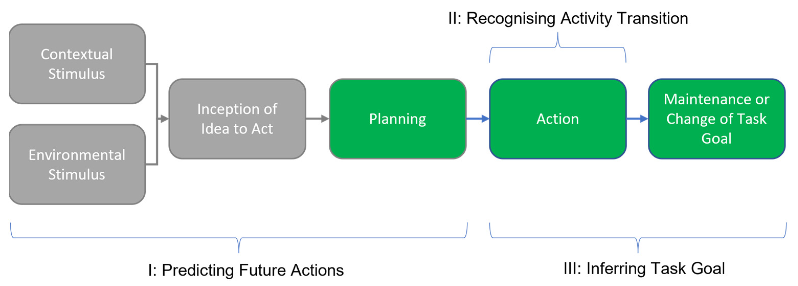
A user’s intent may be broadly thought of as the action they would like to happen at a given time. It can be defined as consisting of three aspects: (i) the prediction of future activities, (ii) activity transition recognition, and (iii) inference of the task’s goal [1,6,10]. The prediction of future actions involves looking ahead to an activity that has not yet begun to take place (e.g., detecting a staircase ahead, which a user may soon be about to climb). Activity transition recognition involves identifying the user’s current activity and detecting when it changes (e.g., starting walking). Goal inference is concerned with identifying the objective of the current activity (e.g., the user is walking towards the staircase). An overview of these aspects is shown in Figure 1.

The effect of sensor unavailability (through failure, lift-off, etc.) on intent prediction accuracy remains unclear and also directly impacts on the maintenance question. A technology that no longer reaches a certain level of performance needs to be serviced; so, keeping the performance level as high as possible even when components fail will result in a better experience for the user. This study explores how a new modular algorithm compares to more established methods of intent prediction when sensors drop out.

This study investigates all three aspects of intent sensing, with elements of activity transition recognition, inference of a task’s goal, and activity prediction. Analysis was performed in real time, with the intent estimations having continuously updated over the course of the activity. Participants were given advance warning of the actions they were required to perform to allow the possibility of an anticipatory response to occur [11], which was used to predict the action itself. The activity transition was then detected, and any change in task goal was monitored, resulting in a holistic intent-sensing system. At the moment, these systems are still rare in the literature [1], and different algorithmic approaches can be used to predict the action. The different options for this are discussed and compared.

1.3. Intent Sensing Methods: Modular and Non-Modular

Current multi-sensor control systems for prosthetics generally tend to favour a combined, non-modular method (NMM), where the system is trained on a specific combination of sensors that are available, and therefore, suffers from a serious reduction in accuracy when the sensors become unavailable. The choice of algorithm used can affect the extent to which this occurs: a K-Nearest Neighbours (KNN) classifier, for instance, is generally more robust to sensor dropout than a Decision Tree classifier is. A modular method (MM), however, might be the most optimal choice for dealing with sensor dropout, as each sensor is trained individually and makes its own prediction, which is then combined with the others at the end of the process using Naïve Bayes techniques. Removing a sensor naturally reduces the accuracy of the system, but the reduction is dependent on the contribution of that specific sensor and does not have a wider impact on the classification algorithm. As such, the decrease in accuracy from sensor dropout is expected to be smaller than it is in a combined, NMM system.

However, without dropout, combined NMMs, which use all sensor inputs to train a single classifier, should perform with a higher accuracy than the equivalent modular approach does, as a combined method can exploit the relationships between sensors. The higher dimensionality can allow classification based on concepts such as “when sensor 1 is high and sensor 2 is low, the intent is more likely to be X”, whereas a modular method of treating the sensors separately would not be able to use this kind of relationship.

This suggests that in cases of no sensor dropout, an NMM is expected to classify intent more accurately than an MM can. Once sensors start to dropout, the equivalent MM should decrease in accuracy much less rapidly than that of the NMM does, until it becomes the more accurate method, with this difference subsequently increasing as more sensors dropout.

This was initially investigated in [6], the authors of which tested an MM against an NMM retrospectively using laboratory gathered motion data. This study aims to apply an enhanced version of these techniques in a more realistic, real-time scenario.

1.4. Intent in Real Time

Unlike [6], the analysis performed in this study took place in a simulated real-time scenario. This means that all techniques used were carefully chosen to ensure that they would work in real time, and the simulated real time was controlled to ensure the algorithm was never given access to “future” data before the appropriate time. A video of the intent classification being performed on data being “played back” in simulated real-time is included in the Supplementary Materials.

Using simulated real time enabled the data collection to be performed remotely. Running the study fully “online” would have been would have been more ideal, as it would have enabled the quantification of the processing speed and would have allowed for the possibility of “user-in-the-loop” behaviour being captured. However, both these factors are beyond the scope of this study, which aims to develop algorithms for an intent-sensing input and does not extend to testing hardware implementation.

Rather than retrospectively classifying a set of data as one activity or another, the algorithms used in this study classify data continuously; at each time step, they update a set of intent predictions. Each update will include an estimation of the current action intent, predictions for actions in the immediate future, and improvements on the estimations from the immediate past.

It is understood that it is more difficult to predict what the intent will be in the future than it is to estimate what is happening at the present moment and that this in turn is more difficult than estimating what the intent was in the past. The prior work in [6] suggested this relationship between the accuracy of intent estimation and time offset should be approximately monotonic, with the accuracy increasing the later on in the activity cycle intent is estimated.

This study will investigate this relationship further, exploring how accuracy increases from the predictive to retrospective time offsets.

1.5. Experimental Concept

The proposed real-time modular method (MM) was compared to a more standard non-modular method (NMM) in a trial involving human participants. To clearly showcase the potential performance of the proposed algorithms, the experimental scenario was kept as simple as possible, while still satisfying the conditions for sensing intent and remaining representative of a practical prosthetic device. Binary classification was used, and we selected between two possible intent states, the right hand being open or the right hand being closed, which the participant switched between according to a pattern shown to them on a screen. A fine time resolution was used, classifying the open/closed state for each 50 ms window, allowing precise measurements of the effect of time on classification accuracy.

The sensing input used was surface electromyography (sEMG), a standard sensor type included in typical prosthetic devices [12]. Up to four of these sensors were used—which is more than a prosthetic device would usually include—to be representative of the best-case scenario as a starting point.

As this study intends to investigate applications of the proposed algorithms to reducing the need for prosthetic maintenance, sensor dropout was simulated to represent a sensor becoming unavailable (from causes such as sensor failure or electrode lift-off). To achieve this, the inputs of sensors were replaced with recorded pure sensor noise when they failed. This means that the signal contained no information, so could not be used for classification. Established methods exist for detecting sensor signal loss through a variety of causes [13]. The simulated dropout/unavailability was implemented from the start of recording; as for the vast majority of the time, a prosthetic device was in a steady state, with a certain number of sensors remaining active. The event of a sensor actually transitioning from working to not working is very rapid, with minimal contribution to the sensor’s overall accuracy; so, the transition to failing was not considered.

2. Materials and Methods

2.1. Data Collection

The data used here were specifically gathered for this study from seven non-disabled human participants (2 females and 5 males; age 23–60; weight 58–91 kg). The study was performed in accordance with the Helsinki Declaration, and ethical approval was obtained from the Medical Sciences Interdivisional Research Ethics Committee (IDREC) of the University of Oxford (Reference Number: R68585/RE001). All data were anonymized.

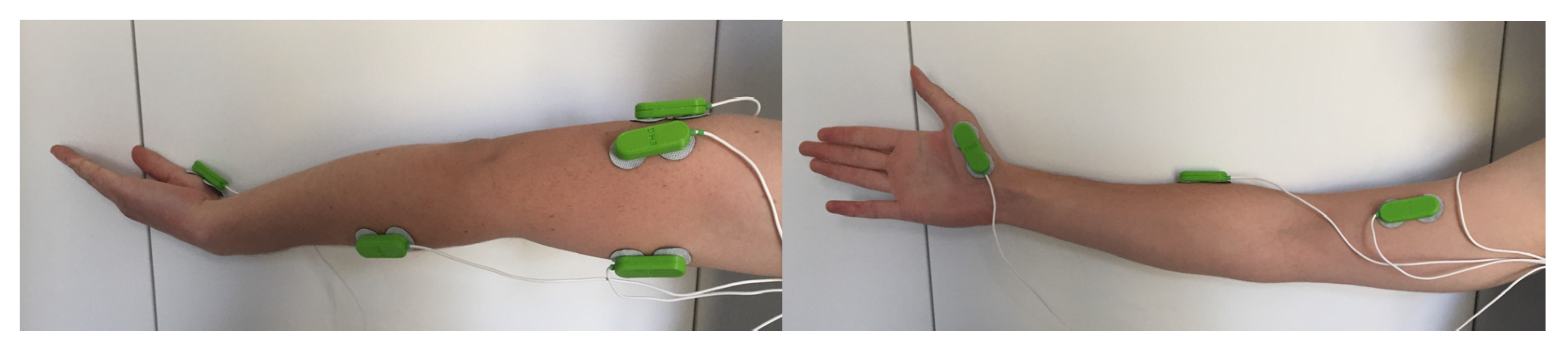
The methodology employed here builds on the method first employed in [14]. Each participant wore four surface electromyography (sEMG) sensors (voltage differential measurement, gain 1009, range +/−1.65 mV, CMRR 80 dB, input impedance 10 G Ohm) connected to a low-cost BITalino (r)evolution body-sensing toolkit, with a sample rate of 1000 Hz [15]. Each sensor module consisted of two gelled self-adhesive disposable Ag/AgCl electrodes (diameter 24 mm, thickness 1 mm, and coated in conductive hydrogel) to be placed on the muscle, and an additional electrode was placed on the collar bone as a ground reference. The sensors were placed on four major muscle sites on the right arm, following standard recommendations from SENIAM—biceps brachii, and triceps brachii (long head and lateral head) [16], along with the extensor carpi radialis. These are shown in Figure 2. Each participant held a finger exerciser [17], with their forearm flat on a table and their palm facing upwards.

A pseudo-random sequence of 1 s and 0 s was generated and presented on a screen in front of the participant as a line graph. This sequence was constrained so that exactly 50% of the sequence was 1 and 50% was 0, with the first 3 entries always being 0. The left edge of the graph was labelled as the “present”, with the future actions the participant would be required to take being shown on the right. Every second, the “future” plot would advance by one time step towards the “present”. The participant was asked to close their hand when the “present” line intersected with 1 and to open their hand when the line was at 0. An audio cue was also used, with a continuous high-pitched tone sounding when the participant was required to close their hand, and a low-pitched tone when they were required to open it.

The sequence used was saved, along with timestamps, to be used as ground truth when the accuracy of intent classification was assessed.

In order to standardise the strength of muscle activation, participants were instructed to close their hand with enough force to fully compress the finger exerciser and no more and to maintain this for the duration of the “1”.

Each trial lasted three minutes, and each of the seven participants was asked to perform three trials, resulting in twenty-one sets of data. To prevent muscle fatigue, the trials were separated by five minutes of rest time.

Additionally, a thirty-minute recording was made to represent sensor lift-off, in which the sensor on the biceps brachii was rotated 180 degrees, so that the electrodes pointed away from the surface of the skin. This meant that the recording was pure noise, with no underlying EMG information. Trials were repeated during this period with the hands opening and closing such as in the ordinary trials, so that motion artifacts could also be included. Sections of this recording were used when sensor drop-out was simulated.

BITalino was connected through Bluetooth to a personal computer running OpenSignals (r)evolution (v2.1.1, Plux Wireless Biosignals, Lisbon, Portugal), which was used to record EMG data.

2.2. Signal Processing

All signal processing was performed in MATLAB (R2022a, Mathworks Inc, Natick, MA, USA). Raw EMG signals were initially filtered with a 10–500 Hz band-pass third-order Butterworth filter and normalised by the maximum filtered signal recorded during training for each sensor on each participant [18].

2.3. Feature Extraction

To interpret the EMG data, protocols established in [19] were followed to represent the industry standard for EMG feature extraction, selecting key features identified in that study. Data were segmented into windows of 200 ms, each shifted by 50 ms, so that consecutive segments overlapped by 150 ms. From each segment, the features extracted were: Integrated EMG, Mean Absolute Value, Mean Absolute Value Slope, Variance in EMG, Root Mean Square, Waveform Length, Autoregressive Coefficients (to the fourth order), Frequency Median, and Frequency Mean.

As this study was performed in real time, an intent prediction was made at the end of each segment, i.e., every 50 ms. For each prediction, the features from the previous ten segments (650 ms) were used, resulting in a total of 110 features for each sensor. These were used to ensure that the full pattern of the changing EMG signal could be recognised and did not introduce input lag, as each segment was labelled according to its delay. This means that, once trained, the system weighted the segments’ contributions appropriately and was predicted to increase accuracy approximately monotonically over time as an activity transition occurred. Further evidence of this is included in Appendix A.

2.4. Real-Time MM Intent Algorithm

The MM algorithm used in this study was adapted from that in [6]. Sensors were treated individually, with no consideration for the relationships between sensors. Training data were used to train an individual KNN classifier for each sensor and to populate a confusion matrix to quantify its accuracy in classifying each possible intent outcome. During testing, each sensor made its own individual prediction of the intent, and these predictions were combined by effectively weighting them according to their confusion matrix entries. This was achieved using Bayes’ rule [20]:

$$P\left(E|V\right)=\frac{P\left(V\vee E\right)·P\left(E\right)}{P\left(V|E\right)·P\left(E\right)+P\left(V|E^{\prime }\right)·P\left(E^{\prime }\right)}$$

(1)

$P\left(E\right)$ is the prior probability of a particular intent being true, and $P\left(E^{\prime }\right)$ is the prior probability of that intent not being true; in this study, both of these are always set to 0.5. $P\left(E|V\right)$ is the probability of that intent being true given the set of sensor values currently being measured. $P\left(V|E\right)$ is the probability of measuring the current sensor values given that the intent being considered is true. Assuming that there is probabilistic independence between the individual sensors, this can be approximated as the product of the probabilities of each individual sensor. $P\left(V|E^{\prime }\right)$ is the probability of measuring the current sensor values given that the intent being considered is not true.

This equation was used to determine the probability of each possible intent being true, and then the algorithm simply selected the intent with the maximum likelihood given the data. When a sensor dropped out, its contribution was not included in the equation, and no re-training was required.

2.5. Comparison NMM Algorithm

The NMM algorithm used for comparison did not require the training of a confusion matrix, and it simply required all training data to be fed into a KNN classifier. When sensors dropped out, their entries were replaced with pure sensor noise, but their dimensions cannot be removed from a combined algorithm; so, the accuracy was expected to rapidly decrease.

2.6. Data Separation

Leave-one-out cross validation was used, which separated data into a training set of twenty samples and a testing set of one sample. Each sample contained three minutes of data. For the NMM, all data in the training set were used along with the recorded ground truths to train a single KNN classifier, which was then used to classify data in the testing sample.

For the MM, a separate classifier had to be trained for each sensor, and each classifier also required a confusion matrix, indicating its sensitivity and specificity. To ensure these were accurate and non-biased results, the same data could not be used both to train the classifier and populate the confusion matrix. The training set was, therefore, subdivided into a classifier training set and a probability learning set.

The classifier training set was used to train a KNN classifier for each sensor. This was then tested on the probability learning set and compared against the ground truth. The results of each classification were tallied and divided by the number of samples to produce the entries for the confusion matrix for each classifier.

The confusion matrix entries then gave the weighting for the contribution of each sensor to the Naïve Bayes sensor fusion algorithm, combining together the individual predictions from each sensor to produce a final prediction for the MM algorithm.

The two algorithms were then used to predict the intent for each segment in the testing set, with the number of successful classifications divided by the number of segments to give the accuracy. This is the metric that has been plotted in the graphs in the Results Section.

2.7. Time Offset

In order to measure the effect of changing time offset on classification accuracy, the recorded ground truth was shifted in increments (T) of 100 ms from −500 to +500. This had the effect of training the system to use each set of ten segments to predict the user’s intent, T segments, in the future for negative values and in the past for positive values.

The classification accuracy of samples in the testing set was measured for each value of T using both algorithms, with the results plotted. A Spearman’s rank correlation coefficient was calculated in order to quantify how well the trend may be described as monotonic. Where $R\left(P_i\right)$ and $R\left(T_i\right)$ are the ranks of each (i-th) sample in accuracy and time, respectively, and $n$ is the number of samples, this was calculated using:

$$r_s=1-\frac{6\sum {\left(R\left(P_i\right)-R\left(T_i\right)\right)}^2}{n\left(n^2-1\right)}$$

(2)

This value is always between −1 and 1, where 1 describes a completely monotonically increasing pattern and −1 describes a perfectly monotonically decreasing pattern. A value of 0 would indicate no monotonic relationship. This value was used to determine to what extent the following hypothesis is true: that accuracy will increase with greater values of T [21].

2.8. Sensor Dropout

A varying number of sensors, n, in the testing set were then replaced with noise from the pure noise recording to simulate sensor dropout. Both algorithms were trained on the full set of four sensors, but the MM was able to simply not include contributions from dropped sensors in its classification system. The NMM, on the other hand, cannot have dimensions removed; so instead, we continued with these entries, which had been replaced with pure noise.

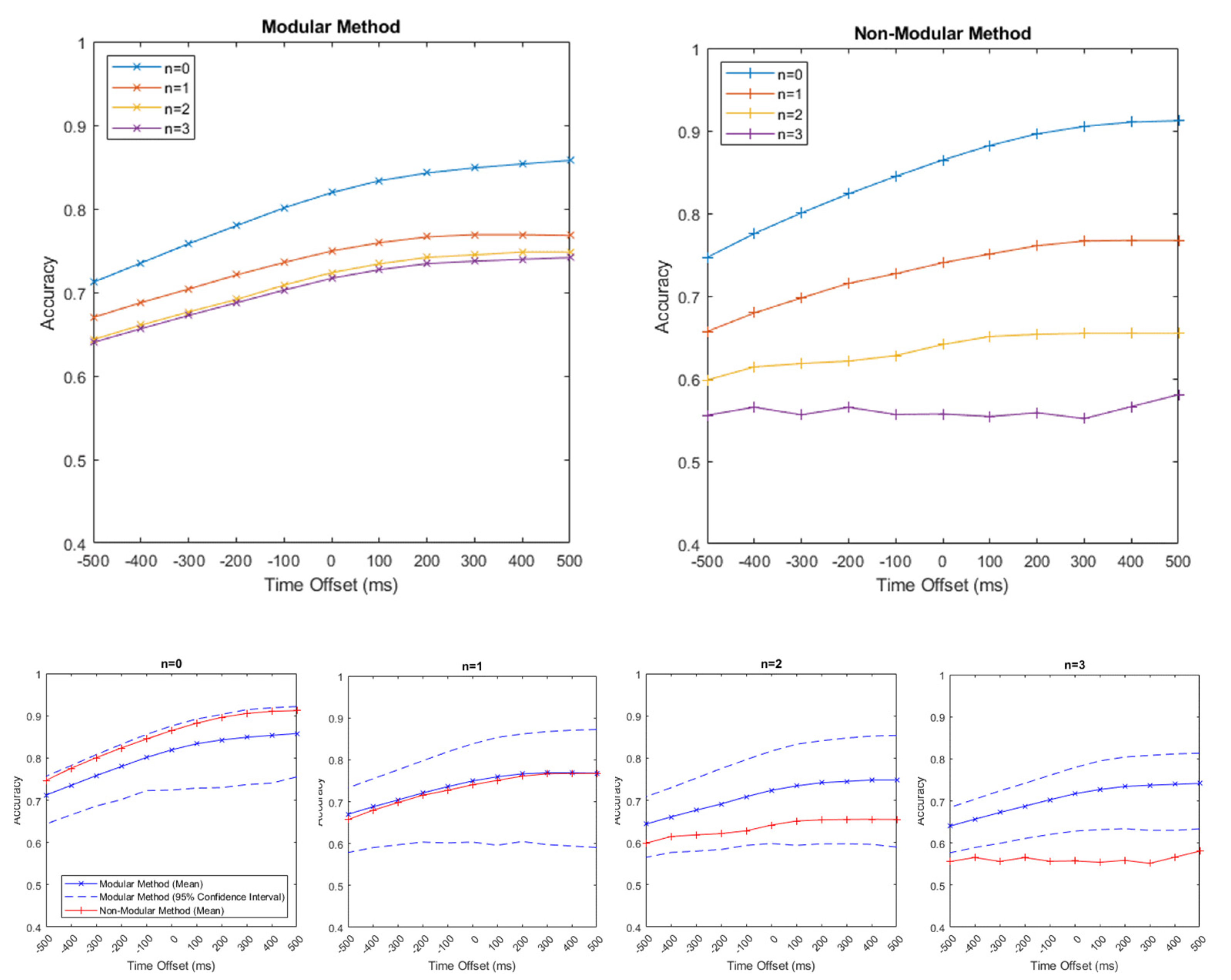
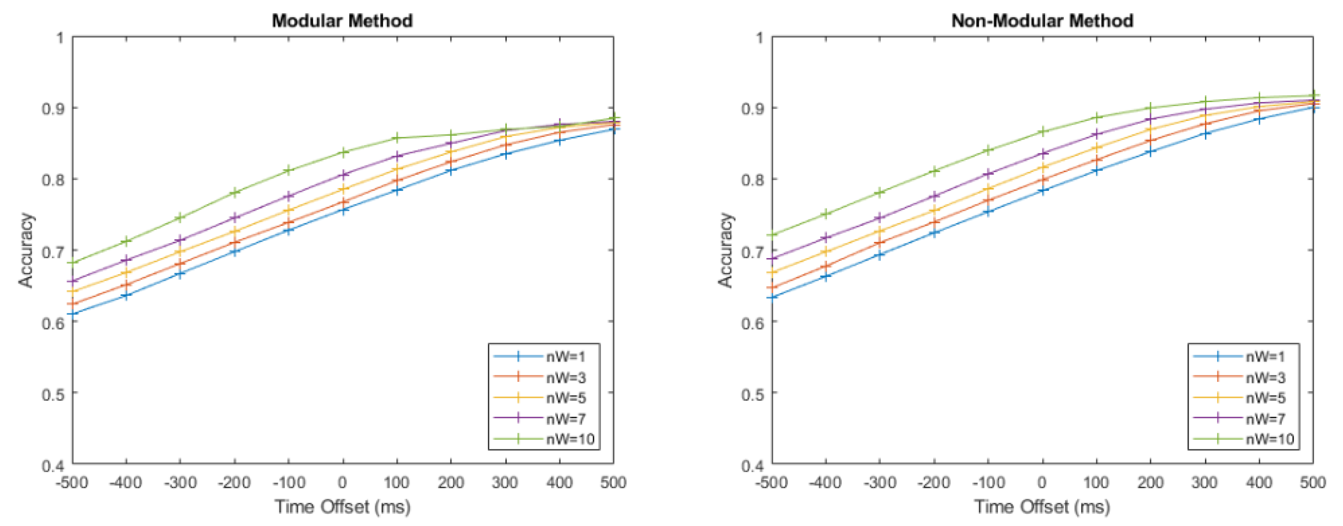
The number of dropped sensors, n, varied from 0 to 3, with classification accuracy recorded at all values of T. This was repeated for every possible combination of dropped sensors, and the mean accuracy was taken and plotted for both the MM and NMM algorithms for all T values. First, the lines of accuracy vs. time offset for values of n were overlaid on two graphs for the MM and NMM, respectively. No confidence intervals were plotted to provide clarity. Subsequently, individual plots were created, comparing the accuracy vs. time offset for the NMM and MM, with one plot for each value of n. For these graphs, the 95% confidence interval for the MM is shown, illustrating the variation in accuracy resulting from the choice of subdivision between the classifier training and accuracy learning sets. No interval is shown for the NMM, as there was no subdivision within its training set, and so, the results are entirely reproducible. The performances for both algorithms were then compared.

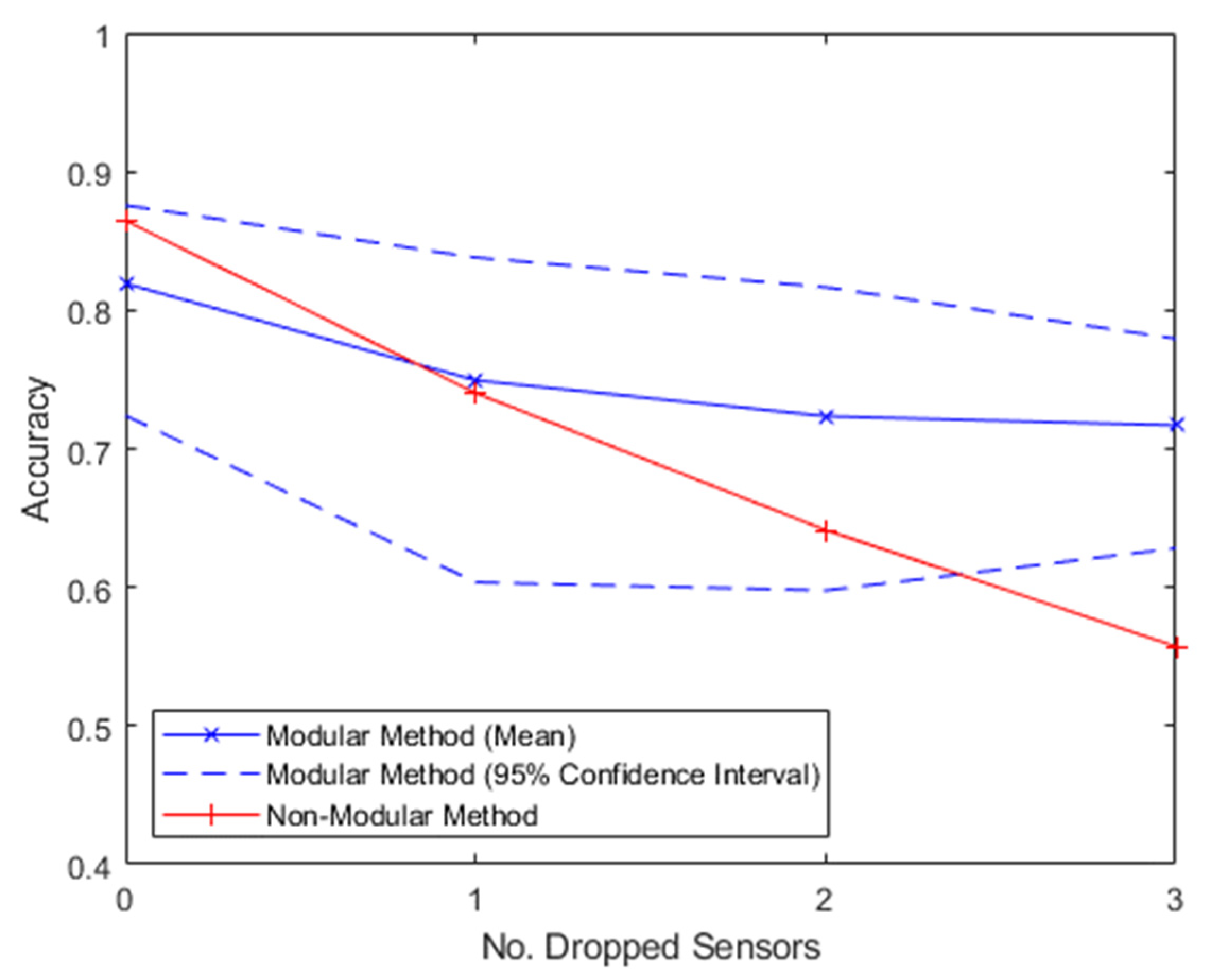
Following this, the time offset was fixed at 0 ms to represent a device predicting the current intent at any given moment. The number of dropped sensors, n, varied from 0 to 3 with all possible combinations for both algorithms. Again, the 95% confidence interval was also plotted for the MM, with no confidence interval plotted for the NMM due to the entirely reproducible results.

3. Results

The results of varying the time offset using the MM and NMM are shown in Figure 3. The maximum accuracies found were 0.91 for NMM and 0.86 for MM (both at zero drop outs), at which point, the gradient had become small, suggesting that these are approximately the maximum accuracies achievable in each algorithm with a positive time offset.

Spearman’s rank correlation coefficient was calculated for each line in order to quantify the extent to which the relationship between accuracy and time offset was monotonic. This is shown in

Table 1. Spearman’s rank correlation coefficients (r_s) calculated for accuracy vs. time offset from n = 0 to n = 3 using the modular method (MM) and the non-modular method (NMM). An r_s of 1 is a completely monotonic increase, 0 is no monotonic increase or decrease, and −1 represents a perfect monotonic decrease.

n	Rs of MM	Rs of NMM
0	1	1
1	0.96	0.99
2	1	0.97
3	1	0.27

.

The resulting accuracy of the MM and the NM, with a time offset fixed at 0 ms, with varying numbers of dropped sensors ranging from n = 0 to n = 3, is shown in Figure 4. Both algorithms were trained on the full set of four sensors. Both plots showed a Spearman’s rank correlation coefficient (r_s) of −1, which indicates a completely monotonic decrease. The mean gradient of the NMM was −0.10/sensor, and for the MM, it was −0.03/sensor.

4. Discussion

4.1. Time Offset

Varying the time offset resulted in a clear monotonic relationship between accuracy and time offset. This demonstrated that the classification of intent is easier when it is conducted retrospectively, and it becomes more difficult to accurately perform it in the earlier phases of the activity cycle. Predicting intent before the activity has begun is particularly difficult, and the MM and NMM could only initially achieve accuracies of 71% and 75%, respectively, compared to the maximum accuracies of 86% and 91%, respectively, 500 ms after onset. This difference may be somewhat explained by the nature of the sensing apparatus. EMG sensors operate by detecting the electrical activity in muscles, which can only be used to predict future activity through the anticipatory response: the slight pre-tensing of muscles just before an activity the subject knows they are about to perform [11]. This is not a reliable response, and it only occurs in a short window of time before the activity begins, resulting in low accuracy far in advance of the activity.

This might be improved in a future system by combining sEMG sensors with another sensing modality that is more effective in the predictive region, such as EEG, which could provide additional information in the planning phase by detecting activity in the brain. Contextual factors such as the time of day could also be employed in a real-world scenario, or environmental stimuli may be detected, which may trigger the idea to act. It has been shown that even small changes in the environment can lead to clear differences in motor control [22]. The nature of the experiment performed in this study did consider these, but future studies performed in situ in a participant’s home, rather than under control conditions in a lab, may be able to incorporate factors of this nature.

The monotonic relationship between accuracy and time offset has implications for practical intent-sensing systems. At a basic level, it highlights a design trade-off between accuracy and responsiveness in any intent-controlled device. Utilising a predictive classifier could totally eliminate the lag between a user attempting an activity and an assistive device engaging, which is used to aid them. However, this results in a lower accuracy of intent prediction than that which might otherwise be achieved by waiting a bit longer.

Different applications could benefit from different choices of accuracy versus delay. Systems that require a rapid response, but have low consequences for incorrect classification, might benefit from a “lower” time offset, thereby accepting the lower accuracy level. Systems requiring a higher accuracy level might be better suited to a “higher” time offset, thereby accepting the increased lag to achieve a desired outcome.

This is something which could be dynamically shifted during device operation. If the accuracy has been reduced due to sensor degradation, failure, or electrode lift-off, increasing the time offset could help alleviate the reduction. However, the resulting increase in lag would have to be carefully considered, particularly in a human-in-the-loop control system, where the permissible lag may be strictly limited. In prosthetic devices in particular, other studies found that an increase in delay reduced the control effectiveness, with a delay of 100–125 ms having been shown to be optimal [23].

A holistic intent-sensing system covering all three aspects of intent could utilise multiple classifiers with different time offsets in parallel. This would enable the device to initially make a prediction as to what the intent might be in the future, allowing it to perform any necessary preparations ahead of time. As the activity onset occurs, this intent prediction could be updated with a new estimation of the current intent, which the monotonic relationship indicates would be more accurate than the prior prediction would be. As the action then continues, the intent could again be updated using an “after the fact” classifier, thereby recording the intent with an even higher accuracy.

A continuously updating intent detection system of this nature could achieve high levels of responsiveness and accuracy, anticipating and preparing for upcoming actions, and then responding accurately to them once they occur. The “after the fact” classifier could even be used to gradually train and improve the predictive classifier, adjusting and tuning it to the specific user. This would be an interesting area to explore in a future study.

4.2. Sensor Dropout

The hypothesis was also shown to be true that while the NMM initially had a higher mean accuracy in the condition of no sensor dropout, the MM began to display a better mean performance as more than one sensor began to drop out. This occurred for all values of time offset, as observed in Figure 3 and Figure 4.

With n = 1 sensor dropping out, the mean accuracy of the MM was similar to that of the NMM. At all the time offsets, the MM performed slightly better than the NMM did, with this difference decreasing as the time offset increased. However, the NMM’s accuracy remained entirely within the 95% confidence interval for all time offsets at n = 1, indicating that the difference is small and the methods are approximately comparable.

For n = 2, the mean accuracy of the NMM is lower than that of the MM (while it is still within the 95% confidence interval). For n = 3, the NMM accuracy is well below even the lower bound of the 95% confidence interval of the MM, showing a strong difference in accuracy between the methods.

In Figure 4, the two methods are compared at a time offset of 0 ms, which is representative of the common method of predicting current intent using all prior information. This clearly showcases the accuracy of the NMM decreasing much more quickly than that of the MM as the sensors drop out, with the NMM decreasing at a rate of −0.10/sensor compared to the MM’s rate of −0.03/sensor.

These findings indicate that standard NMM techniques, such as those commonly used in existing commercially available systems, deteriorate rapidly when sensors start to become unavailable, justifying the need for more frequent maintenance check-ups.

Conversely, the MM technique experiences much smaller accuracy losses when sensors start to become unavailable. Even with three sensors dropped out, 72% classification accuracy was retained at 0 ms time offset, while the NMM’s accuracy was essentially random, supporting the MM as a viable technique for extending the prosthetic’s functional lifetime beyond the current standards.

In regard to the trade-off between accuracy and lag described in the previous section, if an increase in time offset is used to retain accuracy in the event of sensor dropout, a smaller increase is required in the MM than that in the NMM. For instance, with n = 2 sensors dropping out, if a 65% accuracy is required, the MM can achieve this with a time offset of −400 ms, whereas the NMM can only reach this accuracy level with a time offset of 100 ms. The human reaction time is typically in the region of 150–350 ms [24]; so, this difference is comparatively large.

In practice, it is possible to combine these two techniques into an Adaptive Algorithm, which would utilise the NMM when all sensors are available and switch to the MM when a pre-determined number of sensors have dropped out. This could be employed in an assistive device so that when the device is new and fully functional, the NMM is utilised, and then, as sensors start to drop out, when the predicted accuracy of the MM exceeds that of the NMM, the Adaptive Algorithm switches to use the MM. This “best of both worlds” approach could extend the lifespan of a prosthetic device without compromising the system accuracy when all sensors are active, and it may prove to be very effective for practical prosthetic control.

4.3. Limitations of the Study and Recommendations for Future Work

This study took place under carefully controlled conditions, with all participants performing exactly the same, simple actions: opening and closing their hand. This was useful to clearly illustrate the performance differences between the MM and the NMM algorithms. However, it is not representative of the real-life, day-to-day use of an assistive medical device such as an active prosthesis. A future study might use data gathered over a number of days in participants’ homes to be more representative of the algorithms’ practical performances.

The classifiers used in this study labelled data in only two classes: open or closed. In reality, there are many more possible intents a person might have during their daily activities, and so, the classification problem is much more complex. Dealing with this will require more sensors and more training data. Future work could explore the classification of a larger number of possible intents using a larger data set.

While all the techniques used in this study were performed in simulated real time, with no “future” data ever being used to process each prediction of intent, processing itself was performed offline. Future studies could utilise these algorithms in a “user-in-the-loop” scenario by employing a real output device to determine how this changes the accuracy outcomes.

In order to be representative of the sensors available on a prosthetic device, only EMG sensors were used in this study. However, a wider range of sensors, including Inertial Measurement Units and Smart Home sensors, might be available to users in practice, especially as sensing technologies improve in the coming years. Future work on a holistic intent-sensing system should utilise a wider variety of sensors and sensing environments to improve the performance.

All processing in this study was performed on a PC. If it were to be performed in real time on a real medical device, other factors, such as processor speed, battery consumption, and weight, should be considered. Studies exploring the application of these techniques to real medical devices should take these design limitations into account.

Finally, while the K-Nearest Neighbours approach taken for classification in this study is appropriate for the size and feature richness of the data set, more advanced techniques, such as Convolutional Neural Networks, exist, which could use deep learning techniques to automatically extract features and take advantage of emerging properties. The MM algorithm could utilise these CNN classifiers within its sensor modules and still combine them together using a maximum likelihood method, such as the one performed in this paper. Future studies should explore the performance improvement resulting from the use of state-of-the-art techniques, which would more precisely determine the maximum accuracy achievable in an intent-sensing device.

5. Conclusions

This study has contributed a novel method for combining sensors in a modular fashion to produce a continually updating real-time prediction of intent. This method has been shown to be robust to sensor dropout, a key requirement of the proposed ideal holistic intent-sensing system. Newly gathered data were used to verify the theory that accuracy of intent prediction increases approximately monotonically with time after activity inception.

The results obtained support the MM over the NMM in all measured performance metrics under the condition of sensor dropout. In the context of maintenance, this shows potential for increases in the lifespan of prosthetic devices, maintaining their useability even when one or more of their sensors has become unavailable.

This could have major benefits for those with limited access to clinics, particularly in developing nations, and for those that fund their medical devices privately, for whom extending the prosthetic’s lifespan could result in large financial savings.

There are also environmental implications for a device having an increased lifespan. This partly applies to prosthetic devices, but the intent sensing principles discussed in this paper could also be applied to a wide variety of applications, from healthcare to gaming. Increasing the lifespan of all these devices could reduce wastage and landfill use.

Future studies should look to apply these real-time intent sensing principles in more practical environments, where different sensor modes are available. A particular opportunity for accuracy improvements lies in networking with smart home technology, for which the MM algorithm can be used to allow sensors to “drop in/out” as and when they become available.

The ideal intent-sensing system should take advantage of every available sensor at any given time, as with enough training data, the algorithm used should weigh the sensors optimally, so that adding any sensor, however small its information contribution is, should only ever improve the performance of the system.

Future studies should also look to test these algorithms in a useability study with a “user-in-the-loop” scenario to attempt to quantify the benefits of intent sensing as a control input.

It is believed that, in time, as these techniques are developed, intent-sensing systems of this nature will grow to become ubiquitous in modern technology, with benefits for both the users and designers, as well as the environment.