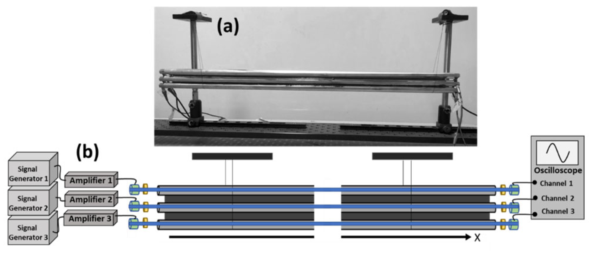
We have conducted an experiment with the system in
Figure 1 by driving waveguides 1 and 3 at the same frequency
and the middle waveguide 2 at a frequency of
The reason for choosing these driving frequencies is that, at these frequencies, the experimental aluminum rod’s (McMaster-Carr 1615T172: diameter = 1/2 inch, length = 0.6096 m, and density = 2660 kg/m
3) longitudinal waves have a wavelength of around 10 cm, making propagation along rod-like waveguides almost one-dimensional [
2]. Additionally, the transducers provide appropriate driving and detecting amplitudes at these frequencies, and the linear longitudinal modes of finite-length waveguides are well-defined [
2]. Initially, drivers 1 and 3 are in phase, and their relative phase,
, is increased by increments of 2.5° up to 360°. The displacement field at the detection ends of the waveguides is Fourier transformed. The Fourier spectrum includes primary peaks at the two frequencies
and
and secondary peaks at multiple frequencies,
, corresponding to nonlinear phi-bit modes. The complex amplitude of each phi-bit mode at the ends of the three waveguides is used to calculate the phase differences
and
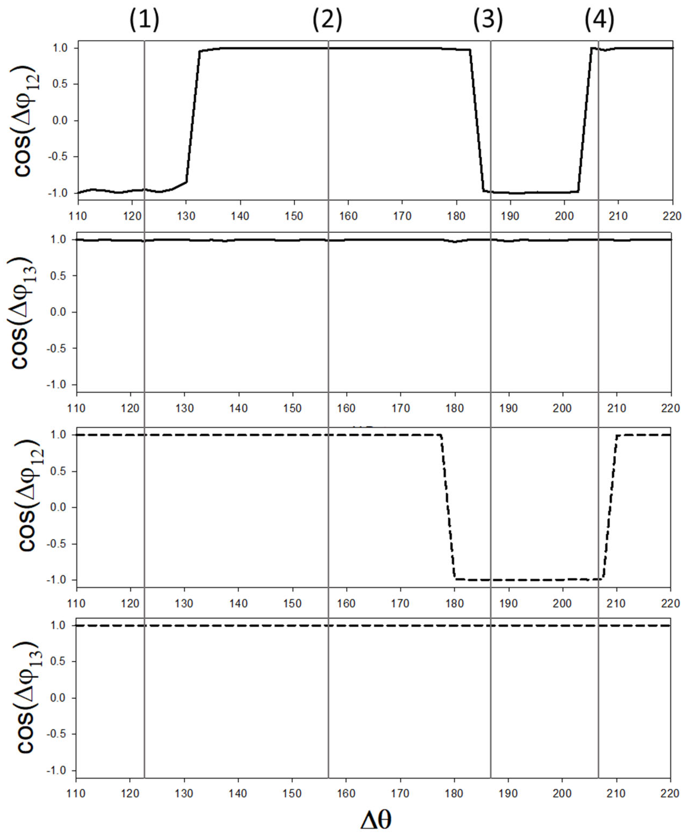
. In
Figure 2, we illustrate these phase differences for two phi-bit modes, namely a phi-bit (a) with nonlinear frequency
({
p = 4,
q = −2}) and a phi-bit (b) with frequency
({
p = 4,
q = −1}). In addition to the response to
of the phase differences
and
, from phi-bits (a) and (b), we have also measured the phases
and
for the primary modes observed at the frequencies
and
. We have also calculated the quantities
and
, as well as
and
. These quantities (
and
, with the superscript 0) would represent the phase differences of the phi-bits if these were simple linear combinations of
and
in the primary linear modes. The response of the two phi-bits is composed of two separate sets of features.
and
of both phi-bits (a) and (b) follow the trend of
,
,
, and
as functions of
. The variations following the linear combinations of primary mode phases will be subsequently called backgrounds. Sharp phase jumps that happen within a few degrees overlap with the backgrounds. These phase jump amount to less than 180°. Similar behaviors are observed for other phi-bit nonlinear modes.
These experimental results broach the challenging questions of the origin of the experimentally observed trends and jumps in the phases and ; this is in the context of enabling manipulation of phi-bit states (Equation (5)) within the Bloch sphere. The subsequent section develops a perturbative model of a nonlinear array of externally driven acoustic waveguides to offer possible answers to this question.
3.1. Model of Nonlinear Logical Phi-Bit and Effect of Drivers’ Phase on Phi-Bit State Vector
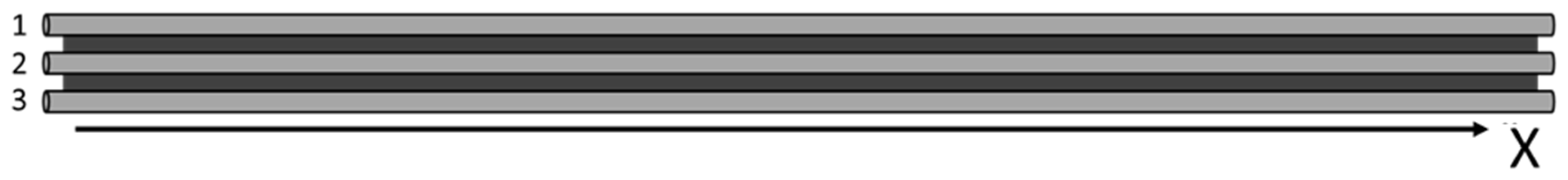
We consider a model of the acoustic metamaterial composed of three one-dimensional elastic waveguides coupled elastically along their length (
Figure 3). Each waveguide is driven externally at its end at the position
.
represents the position along the waveguides.
The nonlinear elastic wave equation in the long wavelength limit is written as
The parameter
β is proportional to the speed of sound along the waveguides. The parameter
represents damping.
is the identity matrix.
measures the elastic coupling strength between waveguides due to epoxy.
is the matrix characterizing the elastic coupling between the three waveguides. In the case of our planar array of waveguides, the coupling matrix takes the form
, , and are 3 × 1 vectors representing the external driving harmonic forces for the three different driving angular frequencies , , and . , , and are the phases of the driving forces.
The displacement in waveguides 1, 2, and 3 is represented by the 3 × 1 vector . is a nonlinear term with strength .
We seek analytical approximations to the nonlinear Equation (6) with three frequency excitations. For this, we consider a variation on that equation that enables us to use frequency detuning with multiple time scale perturbation theory [
11,
12].
Note the additional parameter and the dependency of damping on . A factor of 2 for multiplying the damping parameter is introduced in Equations (6) and (8) to simplify the derivation that follows. The function, , models the nonlinearities that act on the waveguides along their length. It may, therefore, qualitatively represent the effect of the nonlinear elasticity of epoxy.
We introduce two time scales:
and
. We also expand the displacement field as the sum of the zero-order (linear) and first-order (nonlinear) terms, as follows:
. The first-order and second-order time derivatives take the form
The wave equation to the 0th order in
is effectively the linear equation:
Note that there is no damping coefficient in Equation (10) as the effect of damping is now included in the first-order equation. We will see later that the phase associated with damping (included now in the first-order equation) will come back as a correction to the complex amplitude of the zero-order solution.
We can solve this equation by defining
and
with
n = 1, 2, 3: the eigenvalues and eigen vectors of the
matrix, where
represents the spatial eigenmodes across the waveguides with components
,
. We write
The eigenmodes have eigenvalues
and
, and are given by
We now expand the displacement vector on the complete orthonormal basis,
:
The
vectors,
, are also expanded on the basis
:
Inserting Equations (11)–(13) into Equation (10) yields a set of three equations, giving the form of
By employing plane wave expansions, the solutions to the homogeneous equation take the form of
with the dispersion relation:
.
is the
jth wave number for mode
n. The star in Equation (15) stands for the complex conjugate, and the superscript
stands for the homogeneous solution. The summations in Equation (15) cover a discrete set of wave numbers since the waveguides have a finite length.
The particular solutions of Equation (14) that follow the temporal dependency of the driving forces are found in the form
The quantities are real resonant amplitudes. In Equation (16), the superscript stands for a particular solution. In order to obtain Equation (16), we have expanded the cosine functions into complex exponentials.
The complete solution, therefore, takes the form
To obtain a first order in perturbation, the wave equation is given by
Note that the external driving force does not appear in Equation (18) as its full contribution was accounted for in the zeroth order equation. Here, the zeroth order solution now serves as a driver for the first-order equation.
We now choose a form for the nonlinear term
that enables us to proceed analytically and illustrate the effect of the phases
,
, and
on nonlinear modes:
This form assumes that the spatial modes, , do not interact with each other. However, for each spatial mode, the plane wave modes, , may interact with each other. We use a third order nonlinearity for the sake of analytical tractability.
Defining
and using Equation (14), we can rewrite Equation (18) as a set of three equation, each one corresponding to a different spatial mode:
The terms on the right-hand side of Equation (20) can lead to secular behavior.
In order to calculate
, we rewrite equation (17) as
with
. With this, we rewrite the cubic term in Equation (20) as
In this expression, since we have the product of three summations over the wave numbers, we introduced three different wave numbers,
,
,
. However, to simplify the problem, we investigate the self-interaction of one single mode
. We will more carefully examine two types of terms from Equation (22), those that contain the resonant frequencies of the system,
, and those corresponding to the driving frequencies,
. Beginning with those involving resonant frequencies, we seek terms in Equation (22) with a time dependency given by
. These terms will contribute to the secular behavior of Equation (20) and are grouped as
Furthermore, we seek terms in
but without a time dependency of the form
, which correspond to a mixing of the driving frequencies and phases. We focus on terms mixing the frequency and phase of driver 2 with either drivers 1 or 3, which we group as
In order to make contact with the experimental conditions, we now take and , , where is the phase difference between drivers 1 and 3.
In the experiment, since the outer transducers are driven with the same magnitude, and , according to Equation (13), we need to consider two cases. Case I corresponds to the spatial modes for which the are the same, leading to . Case II corresponds to the spatial mode , for which .
In both cases, .
3.1.1. Case I: or 3
In this case, we rewrite Equation (24) in the simpler form:
We now introduce a detuning parameter:
and redefine
as
By regrouping all the terms contributing to secular behavior and setting them to zero, we obtain the relation
Using
, Equations (15) and (16) for the wave number
, and Equations (23) and (26), after some algebraic manipulations, we obtain
where
and
. In Equation (28), the primed quantity is a derivative with respect to
. We have also chosen
without consequence on the rest of the derivation. We now take
. We also define:
such that
. By inserting these into Equation (28) and considering only steady state behavior (that is,
and
), the regrouping of the real and imaginary terms into two separate equations results in
We can get the amplitude-frequency response of the specific nonlinear mode,
due to self-interaction by eliminating the phase
using the trigonometric relation
. That response takes the form of
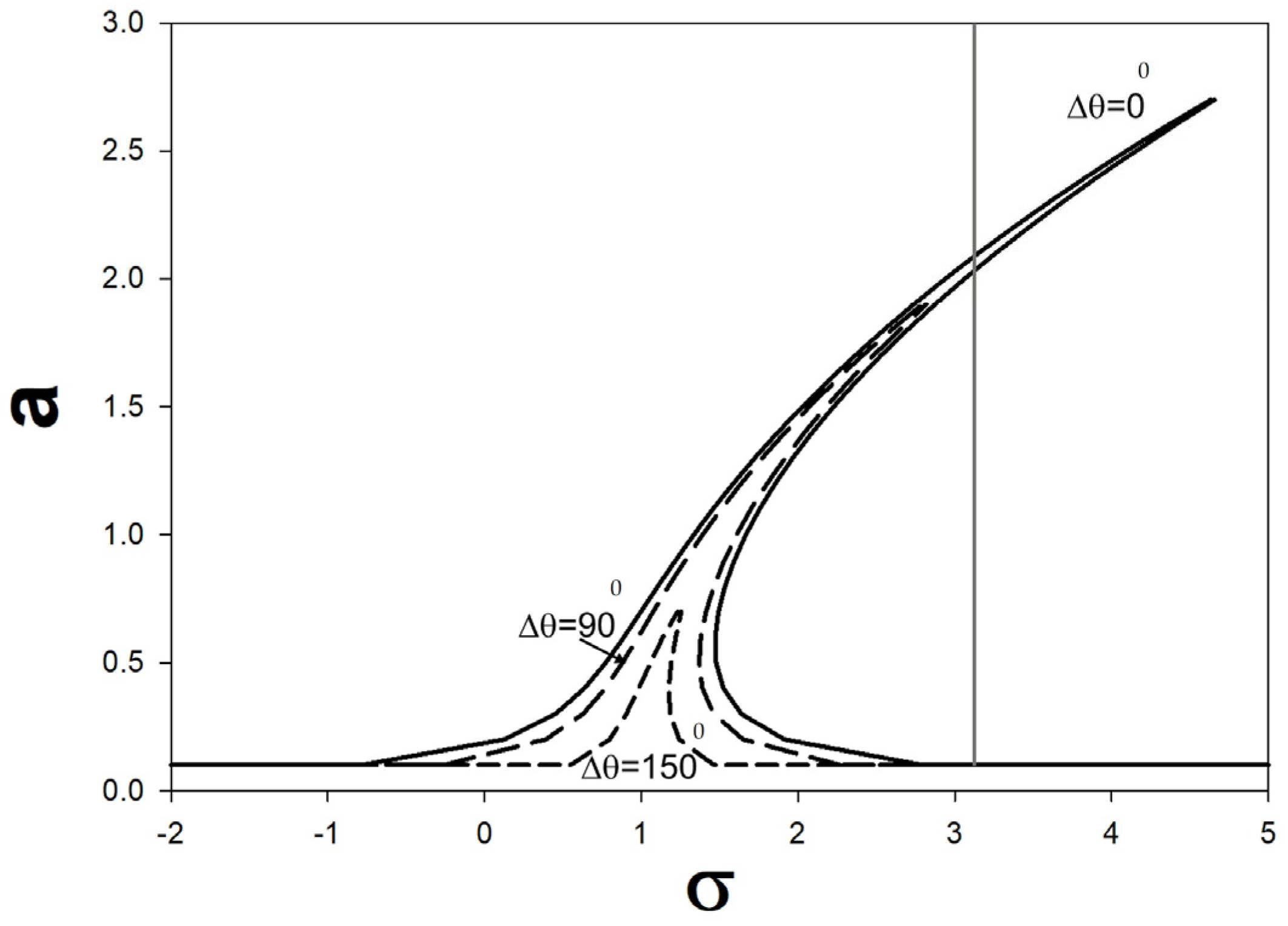
Recall that is the correction to the amplitude solution of the homogenous zeroth order wave equation as a result of the nonlinear perturbation. In some frequency ranges, , the amplitude frequency response may not be a single-valued function. The amplitude may show overhangs to a high frequency or low frequency depending on the sign of . It is centered on the backbone curve given by , where the amplitude decays to zero when . The maximum value of the amplitude is obtained by setting the square root term to zero, . The maximum amplitude is, therefore, dependent on the phase difference between drivers 1 and 3.
In
Figure 4, we note that the amplitude of the nonlinear mode depends on the phase difference between the two drivers, 1 and 3. We note that for
= 180°, the amplitude
a = 0 and the spatial modes
and
do not contribute to the nonlinear correction of the solution of Equation (15). In particular, we note that, at a fixed frequency,
~3.1 (vertical line in the figure), changing the drivers’ phase difference
from 0° to 90° reduces the number of solutions for the amplitude from 3 to 1. This dependency will impact the behavior of the phase,
. We obtain the phase from Equation (29a) as
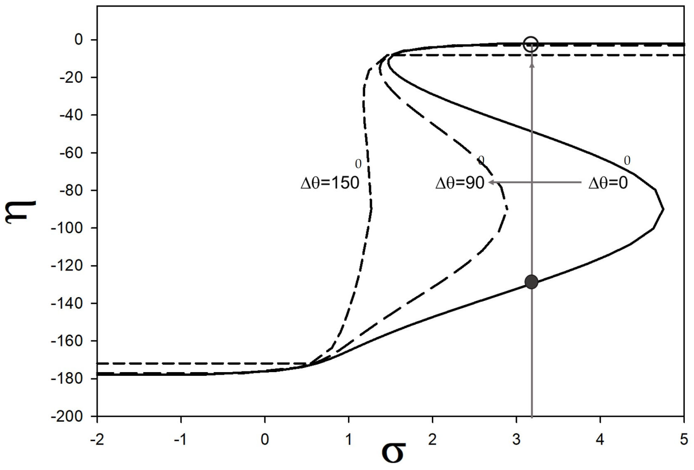
. In
Figure 4, we illustrate the effect of a change in the drivers’ phase on
as a function of frequency. Let us suppose that we prepared the nonlinear mode shown by the closed circle in
Figure 5. This is carried out by setting
and by slowly increasing the frequency
from −2 to 3.1, i.e., by moving along the upper part of the solid line amplitude-frequency response of
Figure 4 up to an amplitude
a~2.0. In that state,
. Increasing the phase difference between drivers 1 and 3 to
reduces the maximum amplitude of the nonlinear mode (long dashed curve) in
Figure 4, which now occurs at a frequency
< 3.
Under this condition, the amplitude-frequency response is single value and corresponds to the state illustrated as an open circle in
Figure 5. This state has a single value
. The change in the driver phase difference leads to a near 130° change in the phase of the nonlinear mode. This jump in phase carries to
through
and
.
Indeed, we can now rewrite
in the form
Here, we are using indices 1 and 3 to specify that the amplitude and phase correspond to the spatial modes
and
. Inserting the definition of:
,
and
, we rewrite Equation (31) as
Considering a single
and
in Equation (21) and focusing our attention on the complex term (keeping aside the complex conjugate in that equation), we obtain
Inserting Equation (32) into Equation (33) yields
The last two terms correspond to the primary linear modes observed experimentally. The first term corresponds to one of the possible nonlinear phi-bit modes, namely {p = 2, q = −1}.
3.1.2. Case II:
In this case, Equation (24) becomes
The secular Equation (27) yields
where again
and
. Choosing
,
and defining
such that
, Equation (36) becomes at steady state (i.e.,
and
)
Equations (37a) and (37b) result from the imaginary and real parts of Equation (36), respectively. Note that in case II, the effect of the phase difference occurs through a sine function instead of a cosine function, as was the case in case I. Additionally, note the swapping between and compared to case I.
We can obtain the amplitude-frequency response of the specific nonlinear mode,
for mode
n = 2 due to self-interaction by eliminating phase
using the trigonometric relation:
. That response takes the form of
This equation has the same backbone curve as that of case 1. The only difference resides in the way the amplitude varies with the phase difference
through
instead of
. Now, for
, that is
, Equations (37a) and (37b) give
a = 0. Spatial mode 2 does not contribute to the nonlinear displacement field. Case II mirrors case I with a
phase lag in
. The second spatial mode contributes to phase jumps in
with, again, a
phase lag in
. Considering a single
in Equation (21) for spatial mode
, we obtain
Again, in Equation (39), we apply a subscript of 2 to the amplitude a and phase to highlight the fact that, in case II, one deals with the spatial mode n=2.
Let us now combine cases I and II. The first-order correction (due to the self-interaction of the wave number to the complete displacement field of Equation (12), ) is now
In the Fourier spectrum of the displacement field, the displacement associated with the nonlinear logical phi-bit mode with a frequency of
measured at
x = 0 is given by
The driver phase difference,
, can, therefore, be used through its impact on
,
, and
to tune the complex amplitudes
and
of a logical phi-bit. These amplitudes may exhibit large phase jumps, which are associated with the phase jumps in
,
, and
, which is a behavior that is consistent with the experimental observation of the sharp phase jumps reported in
Section 3.
We now address the possible origin of the phi-bit phase background as a function of
. Let us consider the particular solution part of Equation (40) evaluated at
x = 0:
In the Fourier spectrum of the total displacement field, the two terms in Equation (42) correspond to the primary modes. We rewrite Equation (42) by introducing
In Equation (43), we have replaced
with
t. As seen in
Figure 1, the array of coupled acoustic waveguides is only part of a system that includes transducers and their ultrasonic coupling agent at the ends of the waveguides. These system components may possess nonlinear as well as damping characteristics, which will be able to mix the frequencies associated with the linear displacement of Equation (43). Indeed, let us consider a model of the transducer/coupling agent component of the system in the form of extrinsic nonlinear damped oscillators at the waveguide ends driven by the displacement
:
where
and
are the characteristic frequency and damping coefficient, respectively.
is the nonlinear function with a strength
.
where the
are displacement degrees of freedom associated with the extrinsic oscillators at the ends of rods,
i = 1, 2, 3.
is some proportionality constant converting displacement into force. Note that since the transducers/coupling agent at the ends of the waveguides are independent of each other, the components,
, in Equation (44) are also independent of each other. So we can rewrite Equation (44) in the form of three independent equations:
In Equation (45), we have chosen the nonlinear function,
in the form of a power
. We can solve Equation (45) using perturbation theory. We seek solutions in the form:
. Regarding the zeroth order in
, the equation reduces to a linear form:
By seeking zeroth order harmonic solutions with the same frequencies as the driving displacement, we obtain
Regarding the first order in
, Equation (45) becomes
Here, the zeroth order solution drives through the nonlinear term to the first-order solution. Inserting Equation (47) into the nonlinear Equation (48) leads to a series of terms with the general form of
, where D is a proportionality constant and
. By focusing on one of these terms, corresponding to one of the logical phi-bits with
Equation (48) yields
A particular solution of Equation (49) may be written as
The fraction prefactors in Equation (50) are the same for each component “
” of
and add the same general phase of each component. Therefore, we have
Note that the coefficients
are real. The Fourier spectrum of the displacement detected by the transducers will include the contribution of Equation (51) to the phase of the nonlinear phi-bit mode, {
p,
q}. These phases are linear combinations of the phase of primary linear modes at frequencies
and
with linear coefficients
p and
q. They will, therefore, contribute the background of the phases of a phi-bit that can be determined from the phases of the primary modes, as was shown it
Section 3. Here, the background in the logical phi-bit phase clearly depends on the parameter
in accordance with the experimental observation. However, to gain full insight into the effect of
on the phi-bit phase, one needs to go beyond the particular solution of Equation (42). Indeed, this solution does not include the effect of damping as it was lumped into the perturbation of Equation (8) in order to use frequency detuning with multiple time scale perturbation theory and shed light on the nonlinear amplitude-frequency response of a phi-bit. In order to illuminate the dependency of the phase of the primary modes, that is, the background of the phi-bit phase, on
, we now reconsider the linear version of Equation (6), with a single driving frequency,
, applied to the three waveguides with different phases, namely
We simplify this equation by working with a complex exponential instead of a cosine function for the driving force. That is, we reformulate the driving force on the right-hand side of Equation (52) as
where we have expressed the phase difference between drivers 2 and 3 relative to driver 1 as
and
. The coefficients
,
, and
are the magnitudes of the forces. We define
. Note that our experiment is conducted with
. However, because we use different transducers for each waveguide, that condition may not be exactly realized.
Expanding
on the basis of spatial modes
,
, and
gives the three components:
We also expand the left-hand side of Equation (52) on the basis of spatial modes; that is, we define . Equation (52) takes the form of three equations, each one corresponding to a spatial mode. We seek solutions for in the form of superpositions of plane waves. The complex resonant amplitudes are obtained for each spatial mode as
,
, and
, where
for
n = 1, 2, 3, wave number,
, and spatial mode eigenvalue,
, as was defined earlier. Inserting Equations (54a)–(54c) into the resonant amplitudes and determining their corresponding phase, as defined by
, yields
These phases are independent of
. We can now redefine
. We note that as
passes through 180° for
r = 1, the phases
undergo a π jump. There is no such jump in
. In order to see how such a jump would carry to a phase jump in the phase of the primary linear mode and subsequently to the background of a phi-bit, we write the complete solution for
:
Note that the
depends on the wave number and eigenvalue of the spatial mode. Since the
correspond to a Lorentzian resonance, we can assume that for a given driving frequency, there might be a single plane wave for each spatial mode that dominates the contribution to
. Choosing also to detect the displacement at
x = 0, Equation (56) reduces to
The components of the amplitude of
are given by
We can now try to evaluate the behavior of
. For instance, we first calculate
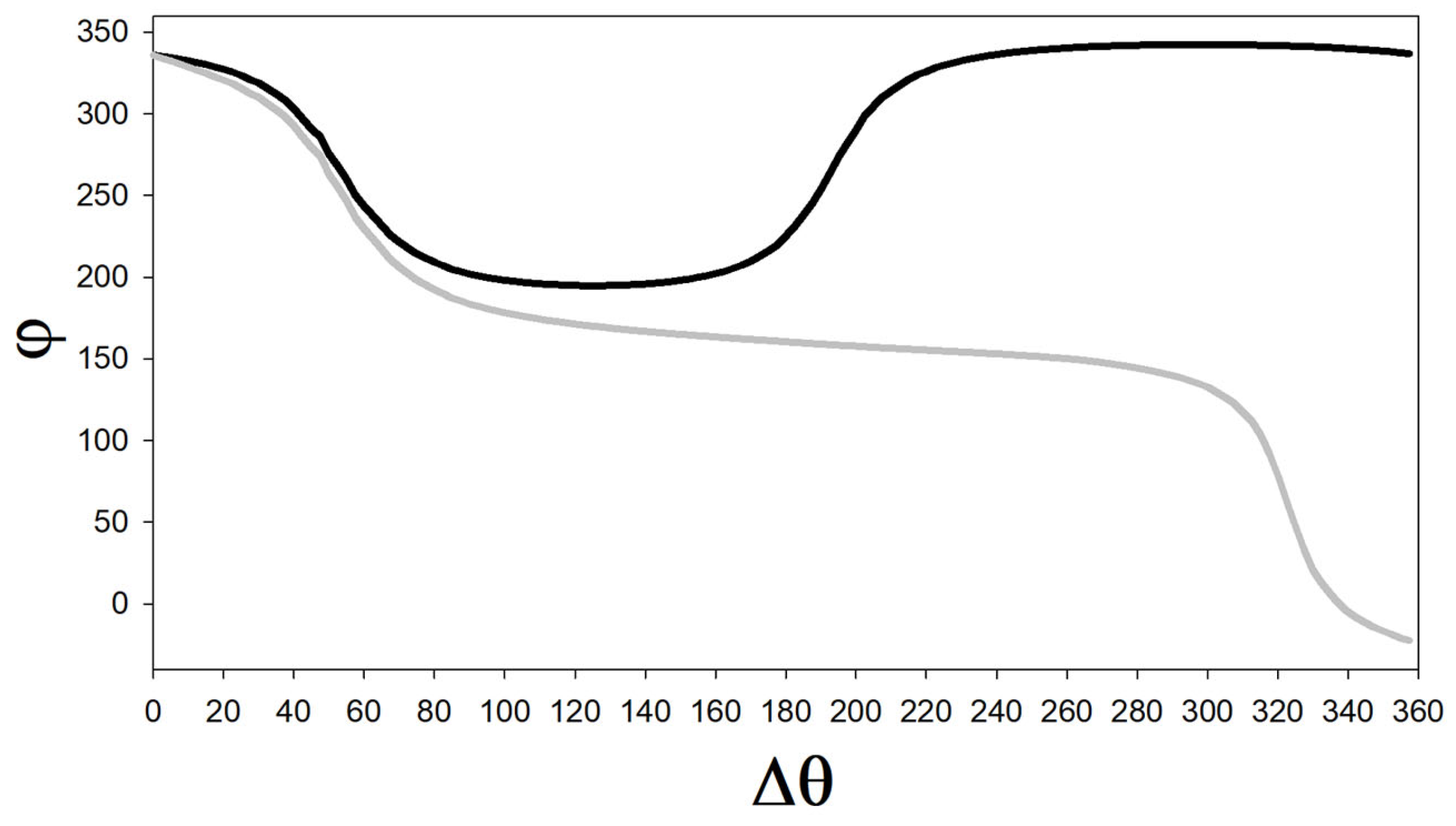
We observe that in this simple model, if we change to , and will effectively interchange. We, therefore, expect no jump in the difference of However, in contrast, a localized change is expected in the difference of . Furthermore, the phases , , and will undergo sharp π jumps when the denominator of the argument of the inverse tangent of Equations (59a)–(59c) becomes zero. Such zeros will not occur for the same value of , leading to several possible phase jumps.
This model indicates that for some specific values of the difference in the phase between drivers 1 and 3,
, one may observe localized changes in the phase of the primary linear modes and subsequently in the background phase of phi-bits (which was shown to be a linear combination of the primary phases). This is consistent with the results of
Figure 2.
In the next sections, we show how we exploit the parallelism of nonlinearly correlated phi-bits and the features of the phi-bit phase (nonlinear phase jumps and background phase) arising from variations in the drivers’ parameter to initialize the state of individual phi-bits and the superposition of states of multi-phi-bits.
3.3. Example of Initialization Using Phi-Bit Background Phase
As seen in
Figure 7 and observed in
Section 2, a background in the phi-bit phase response is common to all phi-bits. This background arises from the phases of the primary mode at the frequency
:
and
. Since
only applies to drivers 1 and 3, which are driven at
, the phases of the primary modes at
,
and
remain constant. Correlations between phi-bits make their background phases react simultaneously to a change in
in the same way.
When considering (for illustrative purposes)
N phi-bits with the same background phases, (we have experimentally verified that in addition to phi-bits (a) and (b) presented in this paper, all other phi-bits investigated possess the same background phases. We recall that the state of each phi-bit “
I” is given by Equation (5):
,
I =
a,
b, …,
m,
n is the phi-bit index. The state of a multipartite composite system constituting
N phi-bits can be constructed as a tensor product of individual phi-bit states,
’s, that is,
. This multi-phi-bit state is defined in an exponentially scaling Hilbert space,
, of dimension
, and can be written as
The basis for that representation is .
In order to construct other complex representations of the multi-phi-bit states, we can apply unitary transformations to the Hilbert space, , which are equivalent to changes in the basis, i.e., a change in the co-ordinate system. Since the experimental background in , and is the same for all phi-bits, we can use different representations to gain the ability to initialize multi-phi-bits states into any desired fiducial state. The choice of representation introduces complexity in multi-phi-bit states composed of identical single phi-bit states by differentiating them.
As an example, let us consider the following three-phi-bit representation:
where
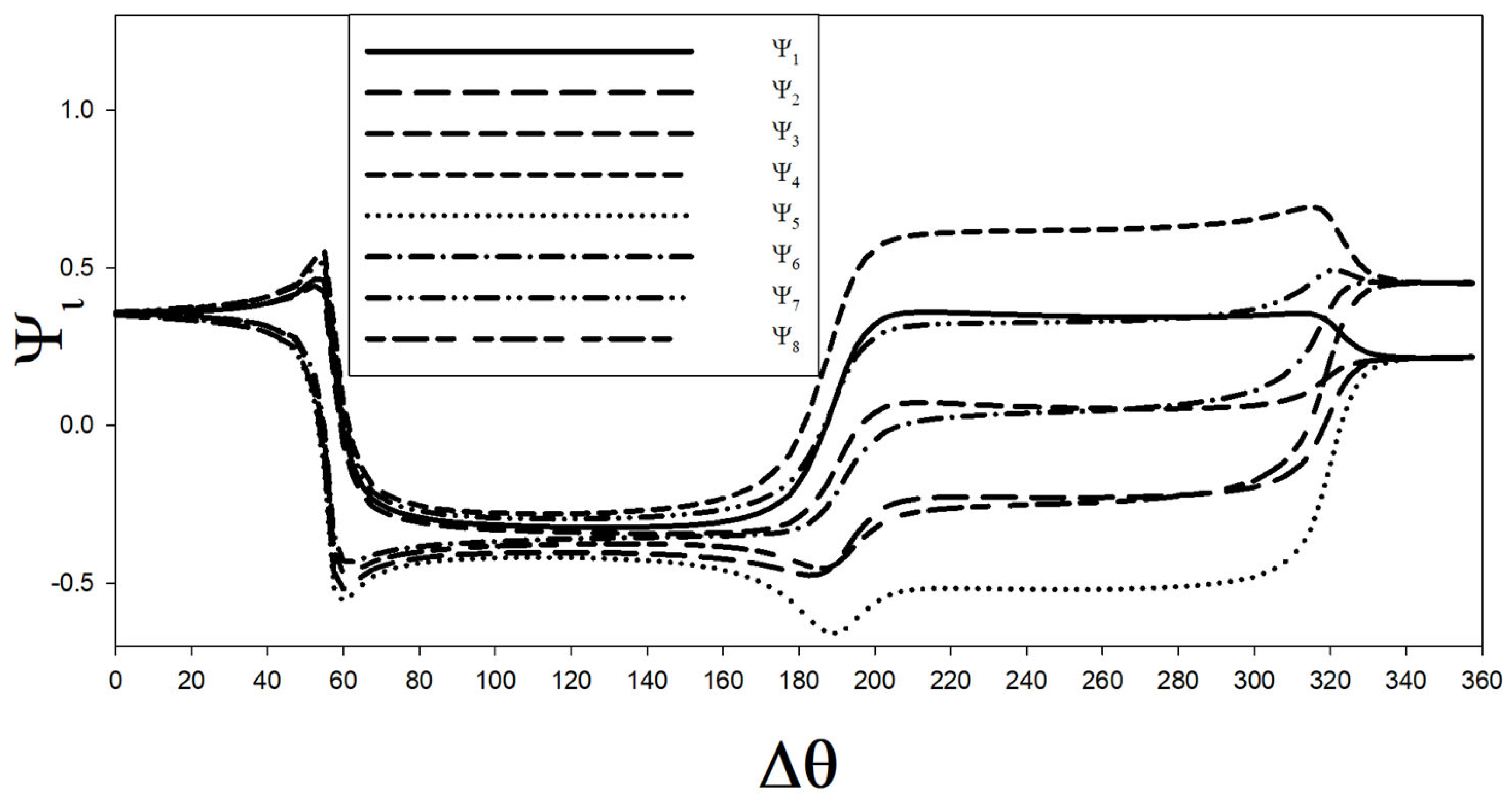
Norm is a normalization factor. In
Figure 8, we report, as an example, these eight components for the set of parameters:
,
,
,
,
,
,
,
, and
. This representation enables the initialization of the approximate states (to within 15%), as expressed in the transpose form
One may notice the simple relations between some of these states, which may be viewed as resulting from nontrivial unitary transformations. For instance,
with, for instance,
This is only an example of the use of representation as a means of initializing multiple phi-bit states. While we are here, we have exploited the background phase of the phi-bit, and we can also use the nonlinear phase jumps in combination with representations to add complexity to the multi-phi-bit states that can be realized. Note that since the phi-bits are nonlinearly correlated, an initializing operation, such as , can be achieved experimentally with a single action of tuning the drivers’ phase difference.


