Effect of a Moving Mirror on the Free Fall of a Quantum Particle in a Homogeneous Gravitational Field

Abstract

We investigate the effect of time-dependent boundary conditions on the dynamics of a quantum bouncer—a particle falling in a homogeneous gravitational field on a moving mirror. We examine more particularly the way a moving mirror modifies the properties of the entire wavefunction of a falling particle. We find that some effects, such as the fact that a quantum particle hitting a moving mirror may bounce significantly higher than when the mirror is fixed, are in line with classical intuition. Other effects, such as the change in relative phases or in the current density in spatial regions arbitrarily far from the mirror are specifically quantum. We further discuss how the effects produced by a moving mirror could be observed in link with current experiments, in particular with cold neutrons.

1. Introduction

The quantum bouncer—a quantum particle falling in a uniform gravitational field bounded by a perfectly reflecting mirror—is one of the paradigmatic examples of quantum mechanics. Mentioned in some textbooks [1,2], the quantum bouncer has been used as a model to investigate wavepacket dynamics and the quantum-classical correspondence [3,4], to derive semiclassical propagators [5,6], and, on the experimental side, to identify the quantized eigenstates of cold neutrons falling on a mirror in the Earth’s gravitational field [7,8].

In this work, we will be interested in the dynamics of a quantum particle obeying the Schrödinger equation with a linear potential (due to a homogeneous gravitational field) falling on a moving mirror. Such a problem belongs to the class of systems subjected to time-dependent boundary conditions. Quantum systems with time-dependent boundary conditions are interesting from a mathematical [9,10], foundational [11,12] or practical [13,14] perspective. Analytical solutions are known only for some special systems [15]. Even the simplest case—an infinite well with a moving wall—needs to be solved numerically [16,17]. Concerning experiments, setups with neutrons falling on a moving mirror have been implemented in order to develop a gravity resonance spectroscopy technique [18] and test exotic theories of gravity [19].

Our aim here will be to investigate some effects induced by moving boundary conditions on the dynamics of a quantum bouncer. Indeed the Hamiltonian remains the same, but the fact that boundary conditions change in a small spatial region imply that the quantum-mechanical wavefunction is modified everywhere, not only in the neighborhood of that small region. This implies that measurable effects (like the current density or the difference in relative phases at a given point) due to moving boundaries can in principle be observed everywhere as long as the wavefunction does not vanish. Such effects were recently investigated in cavities with a moving wall [17] or in confined time-dependent oscillators [12,20]. The original motivation from a fundamental point of view was to look for a novel type of single-particle non-locality [11]. In this paper we will be extending these studies to a particle in free-fall bouncing on a mirror.

To this end, we will first briefly recall the basic features of the Schrödinger equation with time-dependent boundary conditions (Section 2) as well as the main issues that appear when dealing with free fall and moving boundaries (Section 3). We investigate in Section 4 the evolution of quantum properties in the presence of moving boundaries. This will be done by comparing the dynamical evolution of a given initial state in the presence of fixed and moving boundaries. We will compare the short-time as well as the long-time dynamics (relative to the period of a bounce) for different types of initial states. We will particularly focus on the evolution of the current density, the phase, and the probability density of a bouncing wavepacket. We will discuss our results in Section 5, in particular on the prospects for observing experimentally the effects investigated in this work. A short Conclusion is provided in Section 6.

2. Schrödinger Equation with Time-Dependent Boundary Conditions

Before getting to the problem of a quantum particle bouncing on a moving mirror (Section 3.2), let us briefly look at the simplest system with time-dependent boundary conditions: a quantum particle placed in a box, i.e., an infinite well defined along the horizontal x axis, with one of the walls (say the right edge) moving according to some function $L\left(t\right)$. Such a system is defined (see e.g., [21]) by the Hamiltonian

$$H=\frac{P^2}{2m}+V$$

(1)

$$\begin{array}{c}\hfill V\left(x\right)=\left\{\begin{array}{c} 0 \mathrm{for} 0\le x\le L\left(t\right)\hfill \\ +\infty \mathrm{otherwise}.\hfill \end{array}\right.\end{array}$$

(2)

where m is the mass of the particle and $L\left(t\right)$ the position of the moving boundary (here the right edge of the cavity). The solutions $\mathsf{\Psi }(x,t)$ must obey the boundary conditions at $x=0$ and at $x=L\left(t\right)$, i.e., $\mathsf{\Psi }(0,t)=\mathsf{\Psi }\left(L\right(t),t)=0$.

The simplest way to obtain the solutions to Equations (1) and (2) is to view the problem as a Hamiltonian without an explicit time-dependence but with time-dependent boundary conditions. Alternatively one can map through a time-dependent unitary transformation [10] Equations (1) and (2) to a problem with fixed boundary conditions and a time-dependent Hamiltonian; in this case, the usual methods employed to solve time-dependent Hamiltonians can be used.

Keeping to the former method, it is usual to define instantaneous eigenstates of H by

$${\varphi }_n(x,t)=\sqrt{2/L\left(t\right)}sin\left[n\pi x/L\left(t\right)\right]$$

(3)

that verify

$$H\left|{\varphi }_n\left(t\right)\right.〉=E_n\left(t\right)\left|{\varphi }_n\left(t\right)\right.〉$$

(4)

where $E_n\left(t\right)=n^2{\hslash }^2{\pi }^2/2m{L}^2\left(t\right)$ are the instantaneous eigenvalues. Note that these instantaneous eigenstates obey the boundary conditions at $x=0$ and $x=L\left(t\right)$, but they are not solutions of the Schrödinger equation. We define for that purpose functions ${\psi }_n(x,t)$ obeying the Schrödinger equation

$$i\hslash {\partial }_t{\psi }_n(x,t)=H{\psi }_n(x,t).$$

(5)

If these functions are known, then the evolution of an initial wavefunction, say $\mathsf{\Psi }(x,0),$ can be expanded as $\mathsf{\Psi }(x,0)={\sum }_n{c}_n{\psi }_n(x,0),$ and by linear superposition the time-evolved wavefunction will be obtained as

$$\mathsf{\Psi }(x,t)=\sum _n{c}_n{\psi }_n(x,t).$$

(6)

Unfortunately, the basis functions ${\psi }_n(x,t)$ cannot be obtained in closed form except for special choices of functions $L\left(t\right)$; for example for a linear expansion $L\left(t\right)=L_0+at$ the functions ${\psi }_n(x,t)$ have a particularly simple form [22]. For an arbitrary boundary motion $L\left(t\right)$, numerical methods need to be employed. One method is to look for an expansion

$$\sum _n{c}_n\left(t\right){\varphi }_n(x,t)$$

(7)

in the eigenstate basis, but with time-dependent coefficients $c_n\left(t\right),$ that are obtained by solving numerically a system of coupled first order differential equations [16]. This method works efficiently if the coupled system matrix elements decrease to zero fast enough as the basis size is increased; this essentially depends on the scalar products $\left.〈{\varphi }_n\left(t\right)\right|{\dot{\varphi }}_m\left(t\right)\rangle$ (the overdot here and below labels the time-derivative). This is indeed the case [17] for the basis states given by Equation (3).

3. Quantum Bouncer

3.1. Fixed Mirror

The quantum bouncer problem is defined by the Schrödinger equation of a particle of mass m falling on a mirror in a homogeneous gravitational field,

$$ih{\partial }_t\mathsf{\Psi }(z,t)=\left(-\frac{{\hslash }^2}{2m}{\partial }_z^2+V\left(z\right)\right)\mathsf{\Psi }(z,t)$$

(8)

where $V\left(z\right)=mgz$ is the gravitational potential (g is the local free fall acceleration). Placing the perfectly reflecting mirror at $z=0$ implies the wavefunction must obey the boundary condition $\mathsf{\Psi }(0,t)=0$. In order to obtain the energy eigenvalues of the time-independent Schrödinger equation it is customary (e.g., Ref. [3]) to rescale the variables, $z\to z/l_g$, $E\to E/\left(mg{l}_g\right)$ yielding

$$\frac{d^2{\varphi }_n}{d{z}^2}-(z-E_n){\varphi }_n\left(z\right)=0,$$

(9)

whose solutions are well known to be given in terms of the regular Airy function $\mathrm{Ai}\left(z\right)$ by

$${\varphi }_n\left(z\right)=N_n\mathrm{Ai}(z-z_n).$$

(10)

The notation $z_n\equiv E_n$ is chosen because these are simply related to the zeros of the Airy function by $\mathrm{Ai}(-z_n)=0$. $N_n$ is a normalization constant that can be obtained in closed form [4]. The length in these units is given in terms of $l_g={(h^2/\left(2g{m}^2\right))}^{1/3}$, while time is given in terms of $t_g={\left(2\hslash /\left(g^{2}m\right)\right)}^{1/3}.$

The quantized states ${\varphi }_n\left(z\right)$ of a particle falling on a mirror have been observed experimentally with ultracold neutrons [7]. The dynamics of an arbitrary initial state can be easily computed by expanding the initial wavefunction in terms of ${\varphi }_n\left(z\right),$ from which it follows that $\mathsf{\Psi }(z,t)={\sum }_n\left.〈{\varphi }_n\right|\mathsf{\Psi }〉e^{-i{E}_{n}t/\hslash }{\varphi }_n\left(z\right)$. Several dynamical features of eigenstates or wavepackets have been investigated theoretically [3,4].

3.2. Moving Mirror

We assume now the mirror is moving, with its position given by $L\left(t\right).$ Equation (8), as well as the Hamitonian (1) still hold with V now given by

$$V\left(z\right)=\left\{\begin{array}{cc}+\infty \hfill & z<L\left(t\right)\hfill \\ mgz\hfill & z\ge L\left(t\right)\hfill \end{array}\right..$$

(11)

This is similar to Equation (2) implying time-dependent boundary conditions: a solution $\mathsf{\Psi }(z,t)$ of the Schrödinger equation must obey $\mathsf{\Psi }(z=L(t),t)=\mathsf{\Psi }(z=\infty ,t)=0.$ The instantaneous eigenstates analogous to Equation (3) are given here by

$${\varphi }_n(z,t)=N_n\mathrm{Ai}(z-z_n-L\left(t\right)),$$

(12)

but, as above, they are not solutions of the Schrödinger Equations (8)–(11). We have found that their use in numerical schemes is not as reliable as in the infinite well case mentioned in Section 2 due to the properties of the Airy functions: scalar products of the type $\left.〈{\varphi }_n\left(t\right)\right|{\dot{\varphi }}_m\left(t\right)\rangle$ decrease very slowly with increasing m, so that hundreds of thousands of terms would be needed in the expansion (7) for typical parameter values.

Closed-form solutions of the Schrödinger equation with the potential (11) with an arbitrary function $L\left(t\right)$ are unknown except in a handful of special cases [15,23]. One particular case we will be using below is the parabolic motion

$$L\left(t\right)=a{t}^2+bt+c.$$

(13)

The solutions can be shown [15] to be given by

$${\psi }_n(z,t)={\mathcal{N}}_n{e}^{-\frac{im}{2\hslash }\left(2\dot{L}\left(t\right)(z-L\left(t\right))+{\int }_0^t\dot{L}{\left(t^{\prime }\right)}^{2}d{t}^{\prime }-2g{\int }_0^{t}L\left(t^{\prime }\right)d{t}^{\prime }\right)}{e}^{-\frac{i}{\hslash }{\Lambda }_{n}t}Ai\left(\frac{z-L\left(t\right)}{\delta }-z_n\right),$$

(14)

where

$$\delta ={\left[\frac{{\hslash }^2}{2m^2(g+2a\left(t\right))}\right]}^{1/3},$$

(15)

$\ddot{L}=2a$ has to be such that $g+2a>0$, and ${\Lambda }_n$ is related to the nth zero of the Airy function through

$${\Lambda }_n=m\delta \left(g+2a\left(t\right)\right)z_n.$$

(16)

The normalization constant (not given in Ref. [15]) can be found to be given by

$${\mathcal{N}}_n={\left(\sqrt{\delta }{\mathrm{Ai}}^{\prime }\left(z_n\right)\right)}^{-1}.$$

(17)

These functions ${\psi }_n$ form a time-dependent basis over which any initial wavefunction can be expanded through Equation (6).

As a consequence of applying the rescaling $z\to z/l_g$, $E\to E/\left(mg{l}_g\right)$, and $t\to t/t_g$ (Section 3.1), we get $g=2$ and $\hslash =2m$ when expressed in gravitational units. This will give $\delta ={\left[\frac{2}{2+\ddot{L}\left(t\right)}\right]}^{1/3}$, and ${\Lambda }_n=2m{z}_n/{\delta }^2$. Consequently, ${\psi }_n(z,t)$ can be written in scaled units as

$${\psi }_n(z,t)={\mathcal{N}}_n{e}^{-\frac{i}{4}\left(2\dot{L}\left(t\right)(z-L\left(t\right))+{\int }_0^t\dot{L}{\left(t^{\prime }\right)}^{2}d{t}^{\prime }-4{\int }_0^{t}L\left(t^{\prime }\right)d{t}^{\prime }\right)}{e}^{-i{z}_{n}t/{\delta }^2}Ai\left(\frac{z-L\left(t\right)}{\delta }-z_n\right).$$

(18)

Note that these solutions can also be understood as resulting from a transformation to an accelerated frame in which the potential has been eliminated. The apparently non-trivial character of the phase in Equations (14) and (18) automatically follows from the corresponding scale transformation [24].

4. Results

We compare in this section the evolution of a quantum particle prepared in a chosen initial state with a fixed or moving mirror. The initial state will be set to be (i) a basis function of the moving mirror, (ii) an eigenstate of a falling particle with a fixed mirror, or (iii) a Gaussian wavepacket prepared above the mirror. In all cases considered we will assume the mirror moves parabolically according to Equation (13).

4.1. Initial Basis State of the Moving Mirror Bouncer

Let us choose as the initial state the ground basis state of the mirror with parabolic motion, given by Equation (18), $\mathsf{\Psi }(z,0)={\psi }_1(z,0)$.

The subsequent evolution if the mirror follows the parabolic motion is then

$${\mathsf{\Psi }}^M(z,t)={\psi }_1(z,t)$$

(19)

and can be read off from Equation (18): the modulus is an Airy function shifted by the mirror’s motion, while the exponential includes a phase as well as a spatial dependent term. If a and b in Equation (13) have opposite signs, there is a time $\overline{t}$ for which $\dot{L}\left(\overline{t}\right)=0$ at which point the spatial dependence becomes real. This implies the current density should vanish at this time, as can be confirmed by computing

$$j_n^M(z,t)=\dot{L}\left(t\right){\left[\mathrm{Ai}\left(z_n-\frac{(c+t(b+at)-z)}{\delta }\right)\right]}^2,$$

(20)

and hence $j_n^M=0$ everywhere whenever $\dot{L}\left(t\right)=0$.

If we prepare the system in the same initial state ${\psi }_1(z,0)$ but the mirror remains fixed, the ensuing evolution is different. The wavefunction is of course not shifted. By expanding ${\psi }_1(z,0)={\sum }_n{c}_n{\varphi }_n\left(z\right)$ in the basis of fixed mirror eigenstates (10), with $c_n=\left.〈{\varphi }_n\right|{\psi }_1〉$, we obtain the evolution in the fixed mirror case as

$${\mathsf{\Psi }}^F(z,t)=\sum _n{c}_n{e}^{-i{E}_{n}t/\hslash }{\varphi }_n\left(z\right).$$

(21)

Numerical results are shown in Figure 1. The intial wavefunction (Figure 1a) evolves differently when the mirror is fixed or moving. Even for very short times, when the mirror has barely moved, the wavefunction and the current density are appreciably different (Figure 1b). When the mirror reaches its maximum ($\dot{L}\left(t\right)=0$), the current density $j_n^M$ vanishes everywhere in the moving case, but not in the fixed case (Figure 1c). When the mirror comes back at its initial position (at $t=2\overline{t})$, we have ${\left|{\mathsf{\Psi }}^M(z,2\overline{t})\right|}^2={\left|{\mathsf{\Psi }}^M(z,0)\right|}^2$ for the probability density when the mirror moves, but this is seen not to be the case if the mirror remains fixed (Figure 1d); note that the probability density in the fixed and moving mirror cases flows in opposite directions.

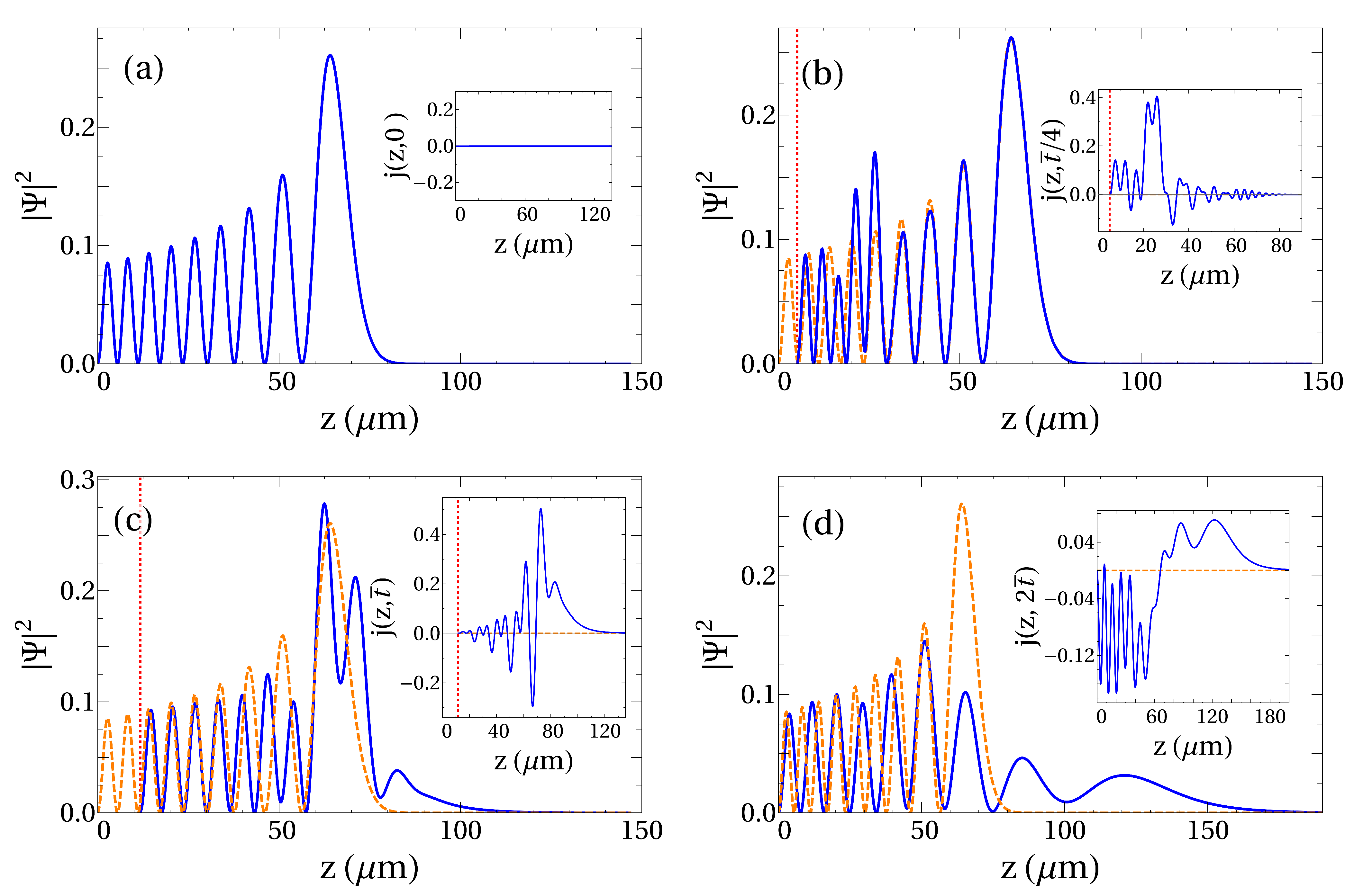
4.2. Initial Eigenstate of the Fixed Mirror Bouncer

We now choose as the initial state an excited state (say the kth excited state) of the fixed mirror problem, so that $\mathsf{\Psi }(z,0)={\varphi }_k\left(z\right)$ as given by Equation (10). If the mirror is fixed, the system remains in the eigenstate and the evolution of ${\mathsf{\Psi }}^F(z,t)$ is trivial. If the mirror moves, we need to expand the initial state in terms of the basis functions $\mathsf{\Psi }(z,0)={\sum }_n{d}_n{\psi }_n(z,0)$ with $d_n=\left.〈{\psi }_n(t=0)\right|{\varphi }_k〉$, and the evolution becomes

$${\mathsf{\Psi }}^M(z,t)=\sum _n{d}_n{\psi }_n(z,t).$$

(22)

An illustration is given in Figure 2 for the $k=9$th excited state. Even for short times, there is a significant difference between the evolution in the fixed and moving mirror cases, as the nodal structure of the moving case is pushed by the mirror at distances far beyond the range of motion of the mirror. Although the highest position of the mirror is $z=11.73$ $\mathsf{\mu }$m, the bouncing particle explores regions of space twice as high than in the fixed mirror case, as basis states ${\psi }_n$ with very high n are populated. Note that the current density, that remains zero everywhere when the mirror is fixed, varies wildly if the mirror moves, including for high values of z.

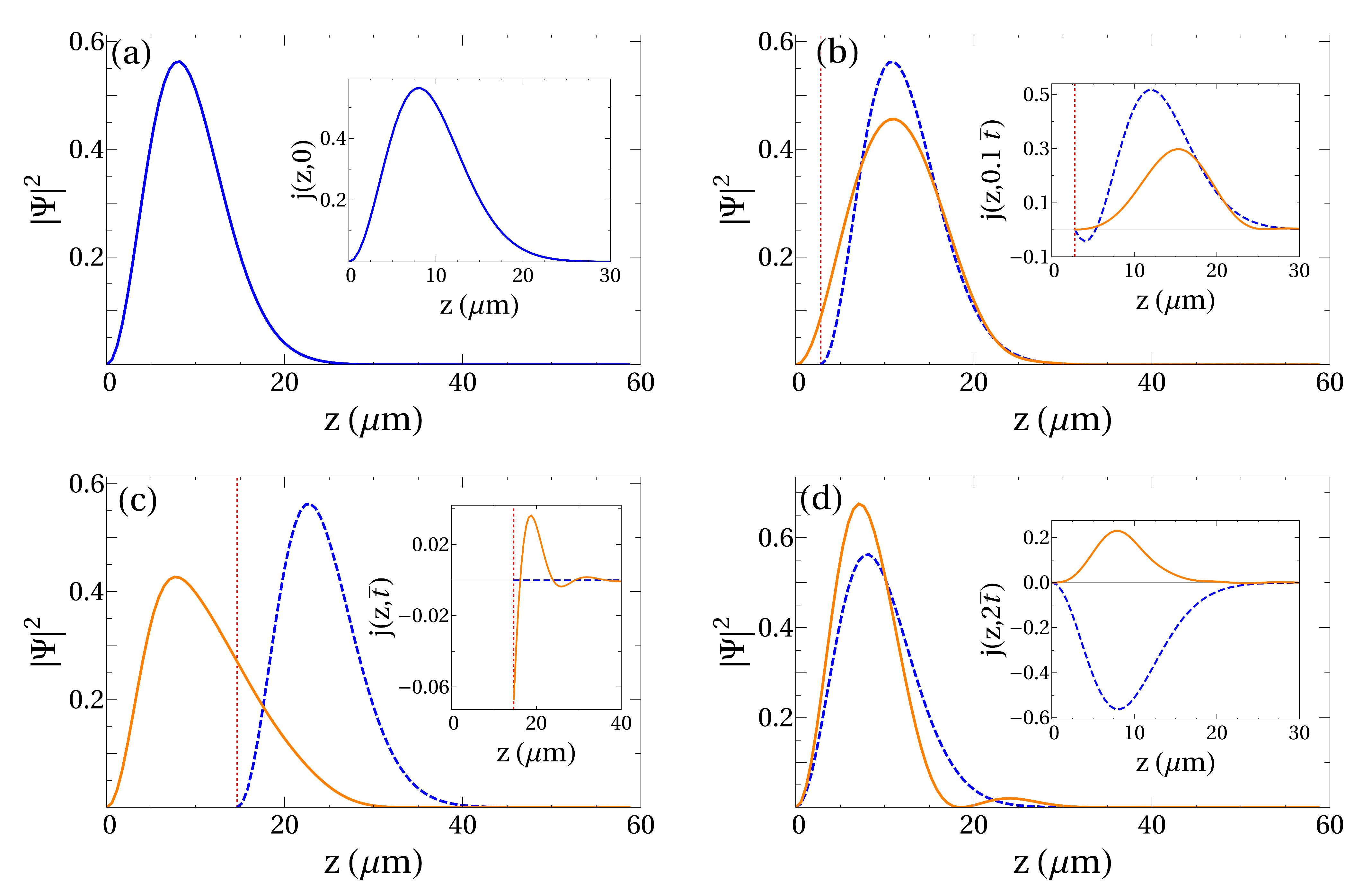
4.3. Initial Gaussian Wavepacket

We finally consider the quantum particle is initially prepared as a Gaussian wavepacket falling with zero average momentum towards the mirror. The initial wavefunction

$$\mathsf{\Psi }(z,0)=\sqrt{\frac{2}{\pi {\sigma }^2}}exp\left(-\frac{{(x-\mathrm{z}0)}^2}{{\sigma }^2}\right)$$

(23)

is expanded over the eigenstates of the fixed miror Hamitonian, in order to compute ${\mathsf{\Psi }}^F(z,t)$, or on the basis function of the Hamiltonian with the moving boundaries, in order to compute ${\mathsf{\Psi }}^M(z,t)$.

The results for a typical example are illustrated in Figure 3, comparing the wavepacket dynamics for a particle initially in a Gaussian state bouncing on a fixed or moving mirror. In this case the mirror moves upwards, kicking the wavepacket to higher altitude than for the fixed mirror bouncer.

5. Discussion

5.1. Dynamical Effects

We have seen for different types of initial states, that the dynamics of a quantum bouncer falling on a moving mirror is different from the bouncer evolution when the mirror is fixed. Some aspects of this behavior can be understood intuitively on classical grounds, for example the fact that the bounce is higher when the particle is kicked upwards by the moving mirror. However there are specific quantum features. These are due to the existence of discrete energy levels of the particle in the gravitational field, and to the fact that the wave needs to adapt globally to changing boundary conditions.

As a result, the effect of the mirror’s motion on the wavefunction and hence on observable properties can be monitored at any point in space. For example the moving mirror populates eigenstates of the gravitational field with higher energies (see Section 4.2), a process that is at the basis of recent proposals [13,14] aiming to implement a spectroscopic method to induce transitions between states. Another striking effect is that the current density may vanish everywhere when the mirror reaches an extremum position, when the initial state is prepared in a basis function state (see Section 4.1). In this situation, we also have ${\left|{\mathsf{\Psi }}^M(z,2\overline{t})\right|}^2={\left|{\mathsf{\Psi }}^M(z,0)\right|}^2$ when the mirror returns to its original position at time $t=2\overline{t}$, but the argument of the wavefunction is almost opposite, i.e., $arg{\mathsf{\Psi }}^M(z,2\overline{t})\simeq -arg{\mathsf{\Psi }}^M(z,0)$ as can be checked from Equation (18) (with $L\left(2\overline{t}\right)=L\left(0\right)$ and $\dot{L}\left(2\overline{t}\right)=-\dot{L}\left(0\right)$). The examples pictured in Figure 1 and Figure 2 clearly indicate that boundary conditions have an effect on the entire wavefunction well beyond the region of changing boundaries.

5.2. Non-Locality

The dynamical features produced by the moving mirror might give rise to non-local effects. The idea that moving boundaries could induce non-locality was proposed by Greenberger [11]. Although Greenberger’s original proposal (based on a wavepacket positioned far from the moving boundary) was disproved [12], it was realized that a quantum state having non-zero probability in the moving boundary region could display non-local features in the sense that an observer located far from the moving boundary region could guess whether the mirror is moving or not before a light ray emitted from the moving boundary region reaches the observer’s position. Note that this instantaneous reaction, albeit small, of the wavefunction to changing boundary condition does not seem to be an artifact of the non-relativistic framework, as it was also seen to be the case for relativistic wavefunctions [25].

In the cases examined in Section 4, non-locality, as defined here, would be obtained provided the dynamical features due to the moving mirror can be observed before a light signal emitted from the position of the moving boundary reaches the point of observation. For instance, when a basis function is chosen as the initial state (Section 4.1), one would need to observe the current density at point $z_0$, or check the relative phase between the inital and time evolved quantum states at $t=2\overline{t}$ (by employing an interferometric setup [20]), in a time shorter than $z_0/c$. When the initial state is chosen to be an eigenstate ${\varphi }_k\left(z\right),$ there are positions $\tilde{z}$ for which ${\left|{\varphi }_k\left(z\right)\right|}^2$ vanishes, while the time-evolved state ${\mathsf{\Psi }}^M(z,t)$ in case the mirror moves will have a small but non-vanishing probability to be detected (see Figure 2); such detections could in principle take place outside the light cone emanating from the mirror position.

5.3. Experimental Observation

Effects produced by a moving mirror on a quantum particle in free fall in a homogeneous gravitational field have actually already been observed experimentally with ultra-cold neutrons [18] when implementing a resonance spectroscopy method. Other effects based on particle counting might be observable with the same technology. The current density could be observed by coupling the neutron spin to the vertical velocity component with a wedge-shaped magnetic field [26], linking the spin deflection to the velocity. Quantities related to relative phases would require interferometry based techniques, the most straightforward option (a neutron bouncing in a Mach-Zehnder interferometer with different boundary conditions in each arm) appearing as hardly realizable.

The observation of non-local aspects appear also difficult to implement with present day technologies (one would actually rather expect on physical grounds to see the breakdown of the wavefunction formalism rather than detection of non-local aspects that could be signalling in certain cases, see Ref. [20]; still, a negative result would be extremely valuable). In principle, the detection of sufficient neutrons (for example by simultaneously measuring on a high number of identical systems the number of detections at a height larger than $\tilde{z}$) in regions for which the fixed mirror case would lead to no detections would be a signature of non-locality provided the detection takes place in a time shorter than it would take a light pulse to reach $\tilde{z}$. However we can see that typical cold neutron eigenstates in the gravitational field, which extend over a few micrometers, would require time delays in the picosecond regime. Not only are these delays minute in order to complete a measurement, but moreover this would require the miror to move at a sizeable fraction of the speed of light. Alternatively, the mirror should move on scales several orders of magnitude below the micrometer regime, which is also unfeasible (and would lead to tiny, probably undetectable effects anyway). The preparation of neutrons in extremely high eigenstates (which would extend over large distances) does not appear to be realistic.

We can rescale the results displayed in Figure 1 and Figure 2 in order to reach regimes for which the moving mirror would give rise to non-local effects. Indeed, reverting the numbers in these figures to gravitational units (see Section 3.1), we see that the light velocity in gravitational units is given by $c(t_g/l_g)=c{\left(4m/\hslash g\right)}^{1/3}$ and decreases for low masses and/or strong gravity fields. For the parameters chosen in Figure 1 and Figure 2, a measurement would have to be made in a time of the order of a gravitational unit $t_g$, for an observer positoned at a few gravitational units $l_g$, so the light velocity would need to be of the order 1∼100 in gravitational units in order for measurements to take place outside the light cone emanating from the mirror. This implies roughly that g/m should be of the order of $c^3/\hslash$, so that for the parameters displayed in Figure 1 and Figure 2 extremely low masses (compared to the neutron mass) and high gravity fields (compared to the gravitational field on the Earth’s surface) would lead to non-local effects.

6. Conclusions

To sum up, we have investigated the effects produced by a moving mirror on the dynamics of a quantum bouncer. We have seen, for different choices of initial states, that a moving mirror modifies the properties of the quantum bouncer, including for short times. Some effects are readily understandable from classical considerations, while other effects are purely quantum, coming form the fact that the wavefunction is modified everywhere by the time-dependent boundary conditions. While in principle the moving mirror could—at least formally—give rise to non-local effects, we have seen that such effects cannot be observed in the regimes accessed by current experiments investigating the behavior of neutrons in a gravitational field. It would be interesting to examine the implications of moving mirrors in the context of the universality of free-fall [27,28,29] as well as in the current experiments investigating the free-fall of anti-matter [30,31].

References

1. Sakurai, J.J. Modern Quantum Mechanics; Pearson: Harlow, UK, 1994. [Google Scholar]
2. Landau, L.D.; Lisfshitz, E.M. Quantum Mechanics; Pergamon: Oxford, UK, 1977. [Google Scholar]
3. Gea-Banacloche, J. A quantum bouncing ball. Am. J. Phys. 1999, 67, 776–782. [Google Scholar]
4. Doncheski, M.A.; Robinett, R.W. Expectation value analysis of wave packet solutions for the quantum bouncer: Short-term classical and long-term revival behaviors. Am. J. Phys. 2001, 69, 1084–1090. [Google Scholar] [CrossRef] [Green Version]
5. Goodings, D.A.; Szeredi, T. The quantum bouncer by the path integral method. Am. J. Phys. 1991, 59, 924–930. [Google Scholar] [CrossRef]
6. Loh, Y.L.; Gan, C.K. Path-integral treatment of quantum bouncers. J. Phys. A Math. Theor. 2021, 54, 405302. [Google Scholar] [CrossRef]
7. Nesvizhevsky, V.V.; Börner, H.G.; Petukhov, A.K.; Abele, H.; Baeßler, S.; Rueß, F.J.; Stöferle, T.; Westphal, A.; Gagarski, A.M.; Petrov, G.A.; et al. Quantum states of neutrons in the Earth’s gravitational field. Nature 2002, 415, 297. [Google Scholar] [CrossRef] [PubMed]
8. Suda, M.; Faber, M.; Bosina, J.; Jenke, T.; Käding, C.; Micko, J.; Pitschmann, M.; Abele, H. Spectra of neutron wave functions in Earth’s gravitational field. Z. Naturforschung. A 2022, 77, 875. [Google Scholar] [CrossRef]
9. Di Martino, S.; Facchi, P. Quantum systems with time-dependent boundaries. Int. J. Geom. Methods Mod. Phys. 2015, 12, 1560003. [Google Scholar] [CrossRef] [Green Version]
10. Mostafazadeh, A. Perturbative calculation of the adiabatic geometric phase and particle in a well with moving walls. J. Phys. A 1999, 32, 8325. [Google Scholar] [CrossRef]
11. Greenberger, D.M. A new non-local effect in quantum mechanics. Physica B+C 1988, 151, 374–377. [Google Scholar]
12. Matzkin, A. Single particle nonlocality, geometric phases and time-dependent boundary conditions. J. Phys. A 2018, 51, 095303. [Google Scholar] [CrossRef] [Green Version]
13. Abele, H.; Jenke, T.; Leeb, H.; Schmiedmayer, J. Ramsey’s method of separated oscillating fields and its application to gravitationally induced quantum phase shifts. Phys. Rev. D 2010, 81, 065019. [Google Scholar] [CrossRef] [Green Version]
14. Duffin, C.; Dijkstra, A.G. Controlling a Quantum System via its Boundary Conditions. Eur. Phys. J. D 2019, 73, 221. [Google Scholar] [CrossRef]
15. Makowski, A.J. Two classes of exactly solvable quantum models with moving boundaries. J. Phys. A 1992, 25, 3419. [Google Scholar] [CrossRef]
16. Glasser, M.L.; Mateo, J.; Negro, J.; Nieto, L.M. Quantum infinite square well with an oscillating wall. Chaos Solitons Fract. 2009, 41, 2067–2074. [Google Scholar] [CrossRef]
17. Matzkin, A.; Mousavi, S.V.; Waegell, M. Nonlocality and local causality in the Schrödinger equation with time-dependent boundary conditions. Phys. Lett. A 2018, 382, 3347–3354. [Google Scholar] [CrossRef] [Green Version]
18. Jenke, T.; Geltenbort, P.; Lemmel, H.; Abele, H. Realization of a gravity-resonance-spectroscopy technique. Nat. Phys. 2011, 7, 468–472. [Google Scholar] [CrossRef]
19. Cronenberg, G.; Brax, P.; Filter, H.; Geltenbort, P.; Jenke, T.; Pignol, G.; Pitschmann, M.; Thalhammer, M.; Abele, H. Acoustic Rabi oscillations between gravitational quantum states and impact on symmetron dark energy. Nat. Phys. 2018, 14, 1022–1026. [Google Scholar] [CrossRef] [Green Version]
20. Waegell, M.; Matzkin, A. Nonlocal Interferences Induced by the Phase of the Wavefunction for a Particle in a Cavity with Moving Boundaries. Quantum Rep. 2020, 2, 514–528. [Google Scholar] [CrossRef]
21. Scheininger, C.; Kleber, M. Quantum to classical correspondence for the Fermi-acceleration model. Phys. D Nonlinear Phenom. 1991, 50, 391–404. [Google Scholar] [CrossRef]
22. Doescher, W.; Rice, H.H. Infinite Square-Well Potential with a Moving Wall. Am. J. Phys. 1969, 37, 1246–1249. [Google Scholar] [CrossRef]
23. Makowski, A.J. On the solvability of the bouncer model. J. Phys. A Math. Gen. 1996, 29, 6003. [Google Scholar] [CrossRef]
24. Cervero, J.P.; Polo, P.P. The one dimensional SchrZXLdinger equation: Symmetries, solutions and Feynman propagators. Eur. J. Phys. 2016, 37, 055401. [Google Scholar] [CrossRef]
25. Colin, S.; Matzkin, A. Non-locality and time-dependent boundary conditions: A Klein-Gordon perspective. Europhys. Lett. 2020, 130, 50003. [Google Scholar] [CrossRef]
26. Rauch, H.; Werner, S.A. Neutron Interferometry; Clarendon: Oxford, UK, 2000. [Google Scholar]
27. Mousavi, S.V.; Majumdar, A.S.; Home, D. Effect of quantum statistics on the gravitational weak equivalence principle. Class. Quantum Grav. 2015, 32, 215014. [Google Scholar] [CrossRef] [Green Version]
28. Emelyanov, V.A. On free fall of quantum matter. Eur. Phys. J. C 2022, 82, 318. [Google Scholar] [CrossRef]
29. Emelyanov, V.A. Non-universality of free fall in quantum theory. arXiv 2022, arXiv:2204.03279. [Google Scholar]
30. Perez, P.G.; Banerjee, D.; Biraben, F.; Brook-Roberge, D.; Charlton, M.; Clade, P.; Comini, P.; Crivelli, P.; Dalkarov, O.D.; Debu, P.; et al. The GBAR antimatter gravity experiment. Hyperfine Interact 2015, 233, 21–27. [Google Scholar] [CrossRef]
31. Doser, M.; Amsler, C.; Belov, A.; Bonomi, G.; Bräunig, P.; Bremer, J.; Brusa, R.; Burkhart, G.; Cabaret, L.; Canali, C.; et al. Exploring the WEP with a pulsed cold beam of antihydrogen. Class. Quantum Grav. 2012, 29, 184009. [Google Scholar] [CrossRef]
Figure 1. Snapshots of the time evolution of the probability density and the current density (shown in the insets) for a neutron prepared in the ground basis state of the moving mirror Ψ ( z , 0 ) = ψ 1 ( z , 0 ) . (a) shows the initial state ( t = 0 ); (bd): The probability density | Ψ F | 2 and corresponding current when the mirror is fixed are shown in orange; the blue dotted lines represent | Ψ M | 2 and j 1 M (inset) when the mirror is moving. The position of the mirror is indicated by a vertical red line. These snapshots are taken (b) at t = t ¯ / 10 ; (c) at t = t ¯ (when the mirror reaches its maximum position); (d) at t = 2 t ¯ (the mirror returns to its initial position). The parameters of the mirror in gravitational units are a = 0.1 , b = 1 and c = 0 , which sets t ¯ = 5 t g . The values shown in the plots have been rescaled from the gravitational unit values by using the neutron mass and the Earth’s surface gravitational acceleration g, giving L ( t ¯ ) = 14.67 μ m at t ¯ = 5.47 ms.
Quantumrep 05 00001 g001
Figure 2. Similar to Figure 1 but when the initial state is prepared as the n = 9 excited eigenstate of the fixed mirror ( Ψ ( z , 0 ) = ϕ 9 ( z ) ) and for a different parabolic motion ( a = 0.5 , b = 2 , c = 0 in scaled units). (a) shows the initial probability density. (b) shows the probability and current densities (in the insets) at t = t ¯ / 4 when the mirror is fixed (dashed orange line) or moving (solid blue). The vertical red line displays the position of the mirror in the moving case. (c): Same as (b) but for t = t ¯ , when the mirror is at its maximum position. (d) shows the same quantities at t = 2 t ¯ when the mirror returns to z = 0 . The values shown in the plots are obtained by rescaling the gravitational units to SI units for a neutron falling in the gravitational field at the surface of the Earth, giving a maximum position of the mirror L ( t ¯ ) = 11.73 μ m at t ¯ = 2.18 ms.
Quantumrep 05 00001 g002
Figure 3. Evolution of an initial Gaussian wave packet released at rest from a height z 0 = 25 l g , and bouncing over a fixed mirror (left panel) or over a moving mirror (right panel). The initial Gaussian is at the bottom (t increases from bottom to top); the red dotted line shows the average position while the parabolic black curve on the right panel indicates the mirror’s position (the parameters of the mirror are in gravitational units a = 0.00625 , b = 0.25 , and c = 0 ). The mirror returns to its initial position at t = 2 t ¯ . We have rescaled the gravitational units so that the numbers on the axes correspond to a neutron falling in the gravitational field of the Earth, leading to z 0 = 146.7 μ m, t ¯ = 21.88 ms and L ( t ¯ ) = 14.67 μ m.
Quantumrep 05 00001 g003
Disclaimer/Publisher’s Note: The statements, opinions and data contained in all publications are solely those of the individual author(s) and contributor(s) and not of MDPI and/or the editor(s). MDPI and/or the editor(s) disclaim responsibility for any injury to people or property resulting from any ideas, methods, instructions or products referred to in the content.