Application of the DMD Approach to High-Reynolds-Number Flow over an Idealized Ground Vehicle

Abstract

This paper attempts to develop a Dynamic Mode Decomposition (DMD)-based Reduced Order Model (ROMs) that can quickly but accurately predict the forces and moments experienced by a road vehicle such that they be used by an on-board controller to determine the vehicle’s trajectory. DMD can linearize a large dataset of high-dimensional measurements by decomposing them into low-dimensional coherent structures and associated time dynamics. This ROM can then also be applied to predict the future state of the fluid flow. Existing literature on DMD is limited to low Reynolds number applications. This paper presents DMD analyses of the flow around an idealized road vehicle, called the Ahmed body, at a Reynolds number of $2.7\times {10}^6$. The high-dimensional dataset used in this paper was collected from a computational fluid dynamics (CFD) simulation performed using the Menter’s Shear Stress Transport (SST) turbulence model within the context of Improved Delayed Detached Eddy Simulations (IDDES). The DMD algorithm, as available in the literature, was found to suffer nonphysical dampening of the medium-to-high frequency modes. Enhancements to the existing algorithm were explored, and a modified DMD approach is presented in this paper, which includes: (a) a requirement of higher sampling rate to obtain a higher resolution of data, and (b) a custom filtration process to remove spurious modes. The modified DMD algorithm thus developed was applied to the high-Reynolds-number, separation-dominated flow past the idealized ground vehicle. The effectiveness of the modified algorithm was tested by comparing future predictions of force and moment coefficients as predicted by the DMD-based ROM to the reference CFD simulation data, and they were found to offer significant improvement.

1. Introduction

The reduction of the aerodynamic drag force remains a core objective of vehicle aerodynamic development and is motivated by the desire to reduce fuel consumption [1,2]. Researchers have attempted to achieve aerodynamic drag reduction through different types of passive flow control devices such as the front bypass ducts [3], rear bypass ducts [4], and various deflector designs [5,6,7]. One of the major limitations of passive flow control devices is that, once installed, they can be difficult to remove or modify. Thus, researchers have turned to active flow control devices to achieve flexibility in optimization [8]. Examples of active flow control include a variety of synthetic jet and suction systems [8,9,10,11,12]; interested readers are referred to the review articles by [13,14] for further details.

Recent technological advances in the automotive industry have shifted the focus of transportation research from human-operated-and-controlled fossil-fuel-based vehicles to electrified (EV) connected and automated vehicles (CAVs). As a result, there is a growing interest in the prediction of aerodynamic characteristics in adaptive driving conditions. An example is platooning, where drag reduction is desired via vehicle-to-vehicle interaction of aerodynamics where one or more trailing cars follow a lead car in close proximity. Active control systems are believed to make platooning feasible for all vehicles, as autonomous vehicles allow for closer proximity due to reduced reaction times [15,16,17]. Before a control signal can be applied to the moving vehicle, predictions of the future state of aerodynamic forces and moments are required. A Reduced Order Model (ROM) can be used to make future state predictions of the aerodynamic flow field [1]. For adaptive systems, the future state predictions can then be coupled with a control input to obtain the desired performance characteristics [18].

Previous studies on the adaptation of aero-devices largely relied upon time-averaged wind tunnel experiments or Reynolds-Averaged Navier–Stokes (RANS)-based numerical methods. Fluid flows around road and race vehicles are highly turbulent and consist of many dynamic coherent structures that are characterized by a wide range of length and time scales. The evolution and convection of these structures produce macroscopic spatio-temporal patterns [1,19,20,21]. Hybrid turbulence modeling simulation approaches, such as the Improved Delayed Detached Eddy Simulation (IDDES), have shown greater success in elucidating these finer vortical structures embedded in the flow field. The challenge with such Scale-Resolved Simulation (SRS) approaches comes from the grid resolution requirements for the high-Reynolds-number flow fields that these methods try to resolve. It is conjectured that the spatio-temporal domain must be resolved to the so-called Taylor scales [21,22,23] in order achieve a desirable accuracy. Thus, such SRS approaches are resource-prohibitive for the onboard controllers on a moving vehicle, as these would likely not have the processing power and time needed to solve a transient flow field while attempting to implement real-time control of the vehicle’s trajectory. As such, there is a need for a Reduced Order Model (ROM) that can provide fast, accurate, and reliable flow predictions utilizing feasible computational resources. Decomposing the fluid flow into its constituent components can be very helpful in this regard. Researchers in this field have largely resorted to methods of modal decomposition to analyze the flow field [1,24,25].

Proper Orthogonal Decomposition (POD) has been a popular method for the modal decomposition of fluid flows [26,27,28,29]. However, the POD modes are arranged by energy and not by dynamical importance, contain a mix of frequencies, and have unclear truncation criteria [30]. In recent times, researchers have used Dynamic Mode Decomposition (DMD), which is a data-driven linearization algorithm that can decompose a set of data into its constituent modes and extract the associated oscillation frequencies of each mode [31]. These constituent modes and their associated oscillation frequencies can then be used to make future state predictions of the system [32,33]. DMD has shown success when applied to a variety of fluid dynamic problems, including water jets [33], backward-facing step [34], circular cylinder wakes [35,36,37], Poiseuille flow, supersonic jet [38], open cavity flows [39], boundary layer flows [36], airfoil, and hydrofoil flows [40,41]. DMD has been seen to be adaptable, and many variants exist. Interested readers are directed to Kutz’s book [24] and Schmid’s review paper [25] for further details.

All of the studies cited above applied DMD to relatively simple flow fields at low Reynolds numbers. A Ground Vehicle (GV) has an associated flow field that is much more complex, and is at orders of magnitude higher Reynolds numbers, which implies a larger spread of length and time scales within the flow field [20,21]. Only a handful of studies have applied DMD to such separation-dominated, high-Reynolds-number flows. Ahani et al. [1] performed DMD on a DrivAer geometry at a Reynolds number of $4.8\times {10}^6$; note that the DrivAer model, developed by [42], is a simplified rendering of a highly complex vehicle geometry. This work was primarily focused on comparing the obtained mode shapes from the DMD to those obtained from the POD. Another study with the DrivAer geometry by [43] performed a low-pass filtering with a cutoff frequency of 10 Hz before the data were processed by the DMD algorithm and thus filtered out all the complexities associated with a high-Reynolds-number flow.

As mentioned earlier, the development of a ROM capable of producing reliable future state predictions will be very useful for the on-road adaptation of the CAVS. However, we needed an engine for this ROM development. Based on the currently available mathematical tools for fluid flow characterization, we anticipated that DMD is a strong candidate. Thus, the objective of this study is to analyze the effectiveness of the DMD methodology in reconstructing the flow field round a moving Ground Vehicle (GV) at a high Reynolds number using data generated from an IDDES-based CFD simulation. Taira et al. [30] states that the weaknesses of DMD include the requirement to obtain time-resolved data with high resolution and determining the metrics to identify dominant modes. In order to obtain such a “reliable” DMD model for high Reynolds number fluid flows, certain parameters pertaining to the DMD requirements must be determined: (a) length of one data-sampling window, (b) data-sampling frequency, and (c) number of data samples for converged ensemble averaging. Additionally, we need to know whether it is necessary to go through the Singular Value Decomposition (SVD) step, as seen in the existing DMD algorithm, and if so, the truncation criteria for the SVD need to be defined. In addition, it is important to know whether the inverse transformation, i.e., the reconstruction of the flow field from the DMD modes, suffers from the artifacts of spurious high-frequency modes or other noise in the training data. As well, we need to know how much flow energy is conserved when the flow field is reconstructed and what is the minimum energy that must be retained when performing a low-dimensional transformation of the system.

In this paper, we attempted to address these questions by applying DMD to a high Reynolds number, separated flow past an idealized road vehicle, the Ahmed body geometry [44]. This choice is driven by the fact that extensive experimental and CFD data are available for correlation and validation of this idealized GV model. Among many variants of the Ahmed Body model, we, however, chose to proceed with the ${35}^{°}$ slant-angle Ahmed body model, as the flow over this model shows all the salient features of the flow over a Sport Utility Vehicle (SUV)-type of vehicle, which is the subject of the next phase of our work [45].

The work flow of this study involves first perming DMD on a canonical 2D cylinder flow at a low Reynolds number to verify and validate the accuracy of the DMD approach to be used. Next, we performed the CFD simulation of the GV and validated the CFD results against published experimental data [44,46]. We then performed a DMD analysis using the data collected from the CFD simulation. Based on our findings on the failure of existing DMD methodologies to produce the desired outcome for such flows, we proposed in this paper: (a) modifications to the CFD data generation strategy and (b) a filtering process for removing spurious modes obtained from the model decomposition. As can be found in the subsequent sections, although not perfect yet, these significantly improved the adaptability of the DMD approach to high-Reynolds-number GV flows.

The subsequent sections further explain the development of the methodologies used and the results that were obtained. The methodology developed in this paper can be applied to generic vehicle shapes, such as the DrivAer, and subsequently to more complex real-life road vehicles to develop ROMs, which can predict on-road characteristics of the vehicle, subject to changes in vehicle operating conditions, such as the CAVs in a platoon.

As a final note, this paper forms a part of the lead author Adit Misar’s doctoral dissertation work [47]. Finally, this paper is approved by the US Army Combat Capabilities Development Command, Ground Vehicle Systems Center (GVSC) as “DISTRIBUTION A. Approved for public release; distribution unlimited. OPSEC#7440.”

2. DMD Mathematical Framework

The first step in the DMD process involves storing the data in a vector form, $X_i^n=\{x_i^1,x_i^2,\dots ,x_i^n\}$. Here, the subscript i represents the i-th element of the grid in which the snapshots of the flow field were taken, and n is the total number of time snapshots collected. Thus, each time snapshot $x^n$ is a vector containing data from all m grid elements at time instant n. If we expand the vectors for the grid elements, we can build the complete dataset in matrix form as shown in Equation (1):

$$X=\left[\begin{array}{ccc}{x}_1^1& \cdots & x_i^n\\ ⋮& \ddots & ⋮\\ x_m^1& \cdots & x_m^n\end{array}\right]$$

(1)

In the DMD approach, the collected dataset from a dynamical system is represented as a coupled system of ordinary differential equations, as given in Equation (2), which itself contains non-linear relations in the spatial and temporal domains.

$$dx/dt=f(x,t)$$

(2)

The idea is to represent data from the non-linear, complex system as a locally linear regression such that $x_{k+1}=A{x}_k$, where A is then chosen to minimize $\parallel x_{k+1}-A{x}_k{\parallel }_2$ over $k=1,2,3,\dots ,n-1$. Since we have collected the data from the system, $x_{k+1}$ and $x_k$ are known, but the function relating them is unknown.

$$x_{k+1}=F\left(x_k\right)$$

(3)

The DMD approach then constructs a locally linear approximation of the dynamical system:

$$\frac{dx}{dt}=Ax$$

(4)

This ordinary differential equation (ODE) form of the dynamical system is advantageous, as with initial conditions, we have a well-known solution:

$$x\left(t\right)=\sum _{k=1}^N{\varphi }_k\exp \left({\omega }_{k}t\right)b_k=\mathbf{\Phi }\exp \left(\mathbf{\Omega }t\right)\mathit{b}$$

(5)

where $b_k$ is the amplitude of each mode, ${\varphi }_k$ are the DMD modes (mode shapes involving the eigenvectors of A), and ${\omega }_k$ are the continuous-time eigenvalues of A. The matrix that results as a product of terms, $\exp \left(\mathbf{\Omega }t\right)\mathit{b}$, is also referred to as the “time dynamics” of the system, as it contains the information associated with the frequency, amplitude, and growth rates for all of the modes. Now, when the dimensions of X are large, A becomes impossibly large to mathematically work with. The existing DMD process circumvents this through eigen-decomposition of A by considering a rank–reduced representation, $\tilde{A}$, which has the same non-zero eigenvalues as A, and is obtained by performing SVD of X using the collected data.

$$X\approx U\mathrm{\Sigma }{V}^{*}$$

(6)

In Equation (6), X is a rectangular data matrix of size $m\times n$, U is a complex unitary matrix of size $m\times n$ that contains the left singular vectors, which are the POD modes, $\mathrm{\Sigma }$ is a rectangular diagonal matrix of size $m\times n$ having a positive real number as its diagonal elements, $V^{*}$ is a complex unitary matrix of size $n\times n$, and ${}^{*}$ represents a complex conjugate transform. The diagonal elements ${\sigma }_i$ of ${\mathrm{\Sigma }}_{ij}$ are the singular values of X. Matrix A may be obtained by using the pseudo-inverse of X, shown in Equation (7):

$$A=X^{\prime }V{\mathrm{\Sigma }}^{-1}{U}^{*}$$

(7)

In practice, since A can be computationally prohibitive to calculate, $\tilde{A}$ is computed through a unitary transform of A as shown in Equation (8):

$$\tilde{A}=U^{*}AU=U^{*}{X}^{\prime }V{\mathrm{\Sigma }}^{-1}$$

(8)

Using $\tilde{A}$, we now can create a low-dimensional subspace of A, such that:

$${\tilde{x}}_{k+1}=\tilde{A}{\tilde{x}}_k.$$

(9)

The eigen decomposition of $\tilde{A}$ can now be computed as:

$$\tilde{A}W=W\mathrm{\Lambda }$$

(10)

where columns of W are the eigenvectors of $\tilde{A}$, and the diagonal elements, ${\lambda }_k$, of $\mathrm{\Lambda }$ are the DMD eigenvalues. We can now use the eigen decomposition of $\tilde{A}$ to reconstruct the high-dimensional DMD modes. The eigenvalues of A, ${\omega }_k$, are expressed in terms of the diagonal elements of $\mathrm{\Lambda }$ (${\lambda }_k$), which are scaled logarithmically according to the relation ${\omega }_k=\ln \left({\lambda }_k\right)/\Delta t$. The eigenvectors of A are given by Equation (11):

$$\mathrm{\Phi }=X^{\prime }V{\mathrm{\Sigma }}^{-1}W$$

(11)

The mode amplitudes may be calculated as:

$$b={\mathrm{\Phi }}^{†}{x}_1$$

(12)

where ${}^{†}$ denotes the adjoint operator, ${\varphi }_k$, and ${\omega }_k$ and $b_k$ may now be used in Equation (5) to obtain the system state predictions. Interested readers are again directed to the original articles and review papers for a more detailed description of the DMD process [25,48,49]. Lastly, Equation (5) can be rewritten as Equation (13) [50]:

$$x_i=\sum _{j=1}^{N-1}{b}_{ij}{\mathrm{\Phi }}_{Norm,j}(x,y)$$

(13)

Kou and Zhang [50] then used this representation to extract a new parameter $I_j$, which denotes the influence of a mode on the entire sampling window as opposed to only at the initial condition. $I_j$ is defined as:

$$I_j=\int |b_j\left(t\right)|\approx {\int }_{i=1}^N\left|b_{ij}\right|dt$$

(14)

The parameter $I_j$ was proposed as an improved method of mode selection. This concept was further modified by Ahani and Uddin [1], and the integral term was replaced with a root mean squared (RMS) term. This new RMS method was used in this paper for mode selection.

3. Methodology

We investigated three cases in this study. Case 1 (C1 here in after) involves a low Reynolds number flow past a 2D circular cylinder. This is a simple and relatively well-known case and was used for initial validation and verification of the DMD process. The second and third cases (C2 and C3, respectively) used the Ahmed body geometry in a high-Reynolds-number flow. Cases C2 and C3 differ in regard to the extents of the computational domain and the associated boundary conditions. Case C2 used Ahmed’s (1984) [44] wind tunnel dimensions as the computational domain. However, the wind tunnel setup used by Ahmed results in a blockage ratio of $4\%$ and necessitates blockage ratio corrections. Since most vehicles are run in an open-air (OA) configuration, we considered it important to switch our Virtual Wind Tunnel (VWT) setup to an OA configuration to better resemble a real-world driving environment. For C3, based on the authors prior experience, the extents of the computational domain were significantly increased [51] to create a computational domain that has a negligible model blockage.

3.1. CFD Simulation Process Details

All CFD simulations were carried out using a commercial finite volume code STAR-CCM+ version 2020.2. For C1, a laminar, incompressible solver was used. The time-step size, $\Delta t$, was set to $0.3\times t^{*}$, where $t^{*}$ represents one Large Eddy Turn Over Time (LETOT). A LETOT is defined as the amount of time required for the freestream flow to pass over the characteristic length of the geometry a single time, i.e., $t^{*}=(t\times U_{\infty })/L$, where $U_{\infty }$ is the freestream velocity, and L is the characteristic model length scale.

As flow case C2 and C3 represent turbulent flows, an incompressible Improved Delayed Detached Eddy (IDDES) solver was used [52,53]. The IDDES approach represents extensions of the original Detached Eddy Simulation (DES) approach proposed by Spalart and coworkers [54,55]. DES is a hybrid approach that combines, for computational efficiency, Large Eddy Simulation (LES) in the regions far away from the wall and Reynolds-Averaged Navier–Stokes (RANS) in the boundary layer region. The switching between LES and RANS is performed by computing a local turbulent length scales, $l_T$, and a local grid size, $l_{LES}$. However, the existing literature reports that LES may incorrectly be applied inside the boundary layer when $l_T$ and $l_{LES}$ drop below a critical value. This can then cause a phenomenon called Grid-Induced Separation (GIS), which is a prediction of nonphysical separation due to the local grid size. In the Delayed DES (DDES) approach, GIS is prevented by introducing a delay in the switching function based on the wall normal distance and local eddy viscosity [56]. IDDES, proposed by [52], is the next extension of the DES, which combines the DDES and wall-modeled LES (WMLES) [57]. In WMLES, RANS is limited to a much thinner near-wall region where the wall distance y is very small compared to the boundary layer thickness, but $y^{+}\equiv y{u}_{\tau }/\nu$ is significantly large; note that with ${\tau }_w$, $\rho$, and $\nu$ representing the wall-shear stress, fluid density and viscosity, respectively, the friction velocity $u_{\tau }$ is defined as $u_{\tau }\equiv \sqrt{{\tau }_w/\rho }$. The IDDES approach was reported to resolve the issue of mismatch between the modeled log layer and the resolved log layer, and it broadened the application area by providing a well-balanced simulation approach for high-Reynolds-number turbulent flows.

The RANS region in the IDDES approach used in this study is solved using Menter’s Shear Stress Transport (SST) $k-\omega$ turbulence model [58,59]. For brevity, mathematical equations related to the RANS, IDDES and SST models are omitted from this paper, as there are plentiful resources for these. Interested readers are referred to the original articles by Menter and coworkers [58,59,60] for the development of the $k-\omega$ model and to the automotive external aerodynamics article by [61] for all relevant equations.

In C1 and C2, a two-layer wall treatment was used to ensure accurate capturing of the boundary layer characteristics. This time-step-independency study carried out by the authors concluded that a time-step size of $\Delta t=1\times {10}^{-4}\times t^{*}$ is sufficient for this setup and is consistent with the time-step size used in previous similar IDDES investigations (c.f. [1,22,62]). To minimize the effects of domain decomposition in CFD predictions, all simulations were run on UNC Charlotte High Performance Computing (HPC) clusters using 144 processors across 3 nodes having 48 processors each [63].

3.2. Geometry, Domain, and Boundary Conditions

For case C1, the circular cylinder with a diameter $D=0.01$ m was placed in the simulation domain. The longitudinal extents of the computational domain were $5D$ upstream and $20D$ downstream of the object. The cross-stream extents were $5D$ on both sides. The upstream edge was specified as a velocity inlet having a stream-wise velocity set to $0.15$ m/s, the down-stream edge was specified as a zero gauge pressure outlet, and the top and bottom edges were specified as zero-gradient boundaries. This setup is found in the user guide of Star-CCM+ version 2020.2, which references the work of Daily et al. [64]. This flow corresponded to a Reynolds number of 75. The C1 case was run for 120 LETOTs, and the last 80 LETOTs of data were used for analyses.

For case C2, the Ahmed body geometry was placed in a VWT of $8L\times 5H\times 5W$ in the stream-wise, vertical and lateral extents, respectively; here L, W and H represents the length, width, and height of the Ahmed body, respectively. These dimensions are similar to the physical wind tunnel used in Ahmed’s original experiment. The vehicle body was placed at a distance of $2L$ from the upstream boundary. Boundary conditions were applied to the computational domain to match the wind tunnel setup of [44,46]. These included a velocity inlet of 40 m/s applied to the upstream face with a turbulence intensity of $0.25\%$, a turbulence length scale of 10 mm, and a 0 Pa gauge pressure applied as an outlet condition to the downstream face, and all other boundaries were specified as no-slip walls. This configuration results in a blockage ratio of $4\%$.

For case C3, the domain extents were significantly increased to $31L\times 35H\times 31W$ in the stream-wise, vertical and lateral extents, respectively, with the Ahmed body placed at a distance of $10L$ from the upstream boundary. The side wall boundaries were changed to a velocity inlet and a pressure outlet to prepare for crosswind simulations, which will be the subject of a subsequent study. This setup for the side-wall boundary conditions is different from the one used by Fu et al. [65], involving turbulence modeling effects on the aerodynamic characterizations of a stock race car subject to yaw, in which a zero-gradient boundary condition was used for the side walls. However, later studies by [51] show that a zero-gradient boundary condition poses nonphysical pressure reflections unless the virtual tunnel is infinitely wide. Finally, to imitate a moving-ground simulation, the floor of the tunnel was given a tangential velocity equal to the free-stream velocity, and the ceiling of the VWT was set as a zero-gradient boundary. This setup was taken from the authors’ experience of performing CFD of crosswind simulations [51]. Both C2 and C3 had a Reynolds number of $2.86\times {10}^6$, which is several orders of magnitude larger than the 2D cylinder case.

For cases C2 and C3, each time-step was run for 10 inner iterations to ensure that residuals had reduced by at least three orders of magnitude. The last 30 LETOTs of data were used for analyses. A C2 simulation was run for 160 LETOTs. It was found that the initial transients subsided after 30 LETOTs. Thus, C3 was run for 130 LETOTs. In both C2 and C3, the last 80 LETOTs were used for averaging and data collection; note that 80 LETOTs correspond to about 2 s of physical time and provide the opportunity to capture a lowest possible frequency of 0.5 Hz.

3.3. Discretization Scheme

The flow case C1 was discretized using polyhedral cells. It has a near wall cell size of $0.05D$ near the cylinder surface, and grows to $0.1D$ elsewhere in the domain. It has five prism layers on the cylinder boundary, resulting in a total cell count of 20,000.

For cases C2 and C3, the simulation domain was discretized using unstructured hexahedral cells. To properly resolve the flow around the GV, five refinement volumes were used around the geometry. The finest mesh was set to a size close to an approximated estimate of Taylor length scale, $\lambda$ [19,22,46]. Further, to properly resolve the boundary layer flows on all the surfaces, a prism layer mesher was used to ensure that the wall $y^{+}$ values are less than unity. In the final mesh, more than 99% of surfaces had a $y^{+}$ value less than unity. For C2, the mesh consisted of $15.24$ million cells. For C3, the meshing parameters are kept the same as in C2, resulting in a mesh of $21.94$ million cells.

3.4. Workflow for DMD Analyses

The step-by-step process required to perform a classical DMD is available in detail in [24]; however, a brief summary of these steps is provided below:

• Step 1: Collect multiple time snapshots of the system of interest.
• Step 2: Create a low-dimensional subspace using the SVD or Truncated SVD (TSVD) method.
• Step 3: Obtain an eigen decomposition of the low-dimensional subspace.
• Step 4: Using the eigen decomposed low-dimensional subspace, assemble the mode shapes and their associated oscillation frequencies, called the “Time Dynamics” (TD).
• Step 5: Use the mode shapes and TD to assemble the DMD output equations.
• Step 6: Use the DMD solution to predict (or reconstruct) the flow field.

3.5. Data Collection Strategy

Storing the entire 3D flow field data associated with all of the time-averaging window time-steps would impractically require more than 3 petabytes of data. Therefore, since we are more focused on the GV aerodynamic force and moment predictions, we collected the static pressure field on the Ahmed body surface. Additionally, to capture the flow field around the GV, we chose eight reference planes around the Ahmed body. For some of these planes, experimental data are available and may be used for future validation steps, such as the wake planes at $x/L=1.077,1.192,1.479$ [20,46]. The other chosen planes are anticipated to capture flow characteristics in critical flow regimes when crosswind and vehicle interaction simulations are to be performed for future investigations. These include planes at $y/W$ = 0.5, 0.88, and 1.27, and at z equal to half of vehicle ground-clearance of 0.5, 1.15, and 1.3 H. Over each of theses planes, seven scalar quantities were collected, viz., pressure coefficient, three components of velocity, turbulent kinetic energy (TKE) or k, vorticity, and the Q-criterion [66]. Thus, instead of storing the entire 3D flow field, we stored only the data from the Ahmed body surfaces and these eight reference planes. Even then, by using this strategy, we extracted about 3.4 TB of data per GV simulation, which is also huge. This is because STAR-CCM+ exports these data in ASCII format with redundancies in exporting spatial locations. Converting the data to binary format and removing the redundancies result in about 400 GB of binary data per case, which is deemed to be a feasible approach. However, this study is limited to the analyses of vehicle surface static pressure data. Note that the CFD simulation time-step size used in C2 implied that the data are sampled at a rate of 4 kHz, and thus, the Nyquist criterion implies that flow structures with frequencies of up to 2 kHz can be captured by the DMD reconstruction.

4. Results

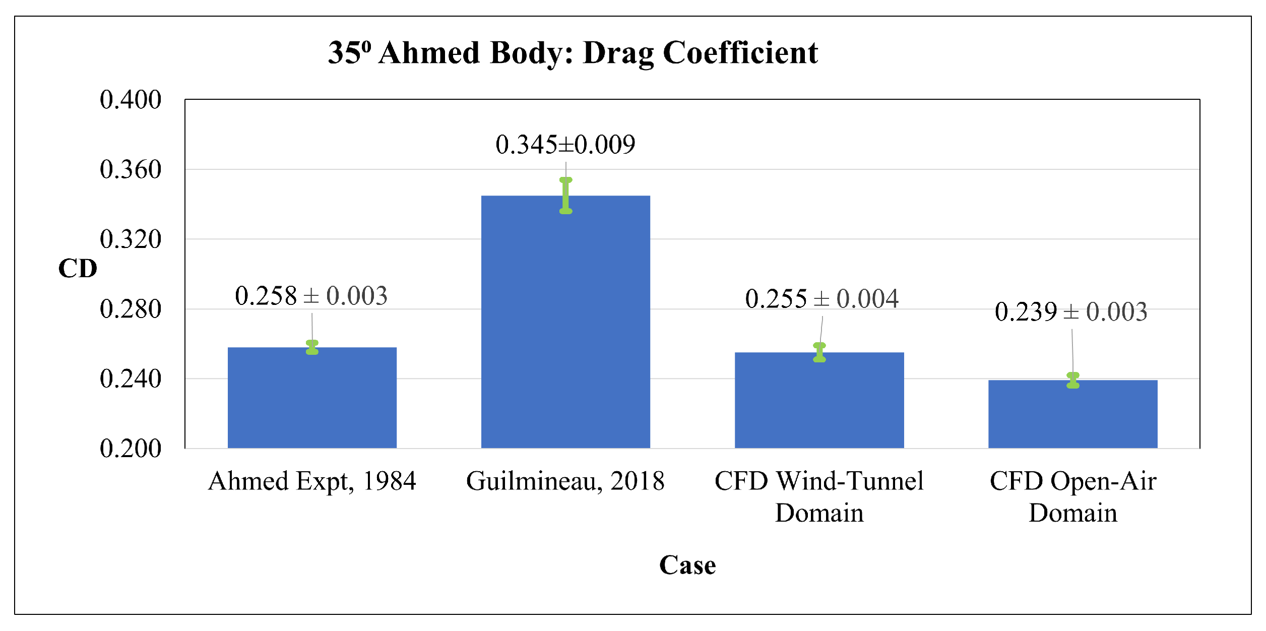
4.1. Validation of CFD Simulation Process

The simulation process used in this study was validated by comparing CFD predictions of the drag coefficient ($C_D$) against the wind tunnel measurements of Ahmed et al. [44], shown in Figure 1, which also contain the IDDES CFD simulation results of Guilmineau et al. [22], as well as predictions using the OA configuration. The error bars in Figure 1 indicate uncertainties for each of the cases. Clearly, our CFD prediction of drag matches very well with the experimental result when the vehicle is placed in a VWT. A 6% reduction in $C_D$ was observed for the OA configuration, which has a blockage ratio of <0.25%. The existing literature suggests that up to a $12\%$ drop in $C_D$ prediction can be expected [67,68].

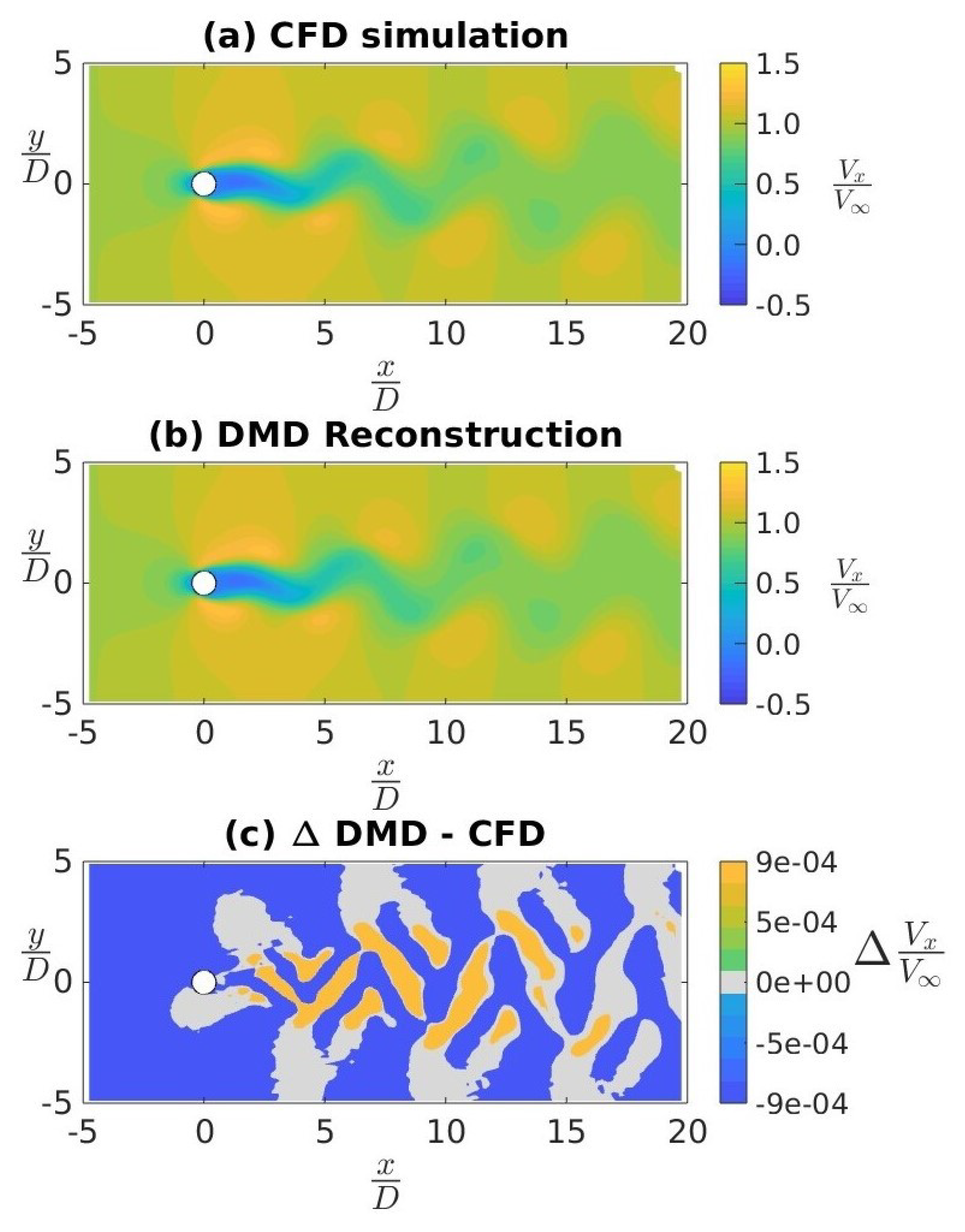
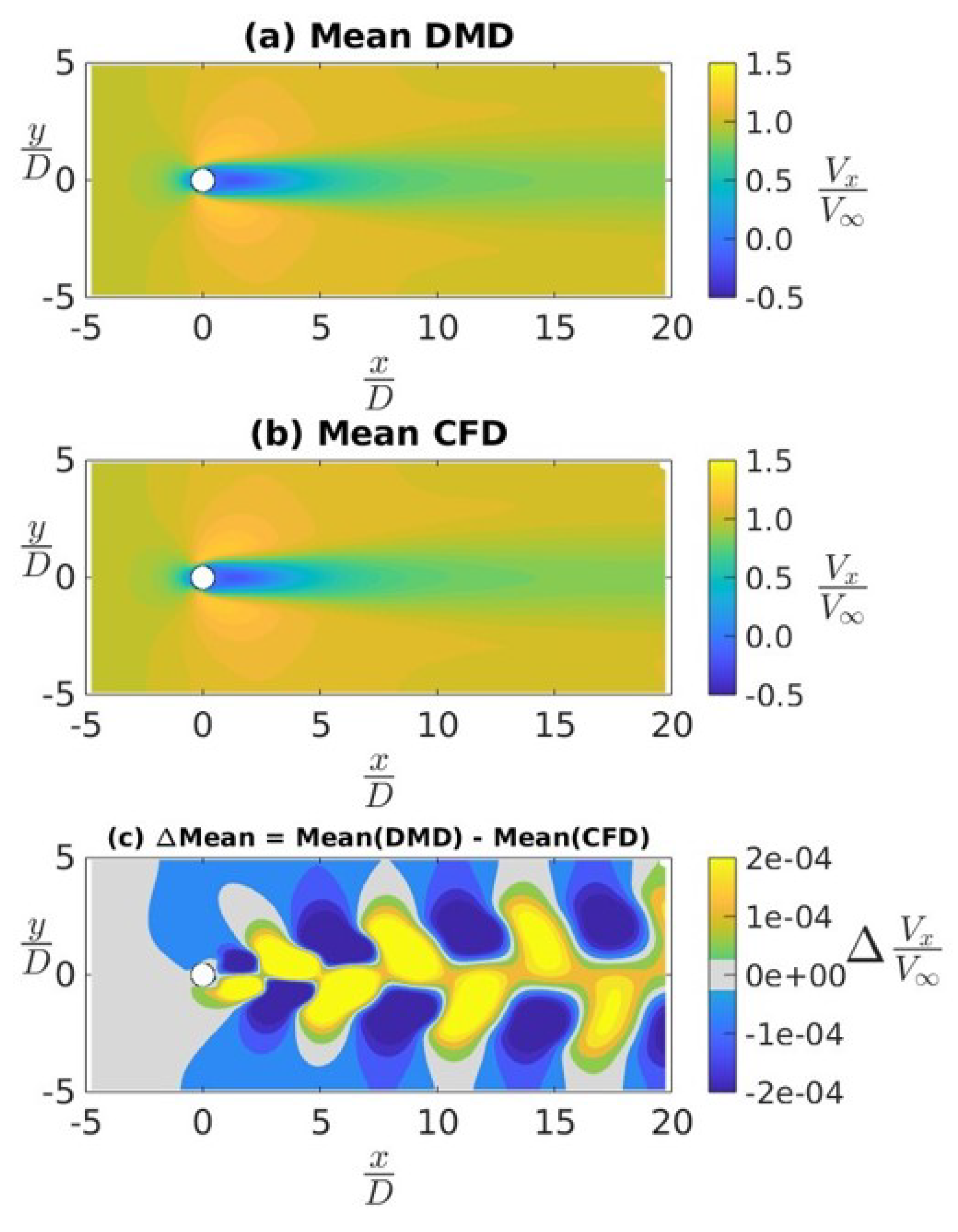
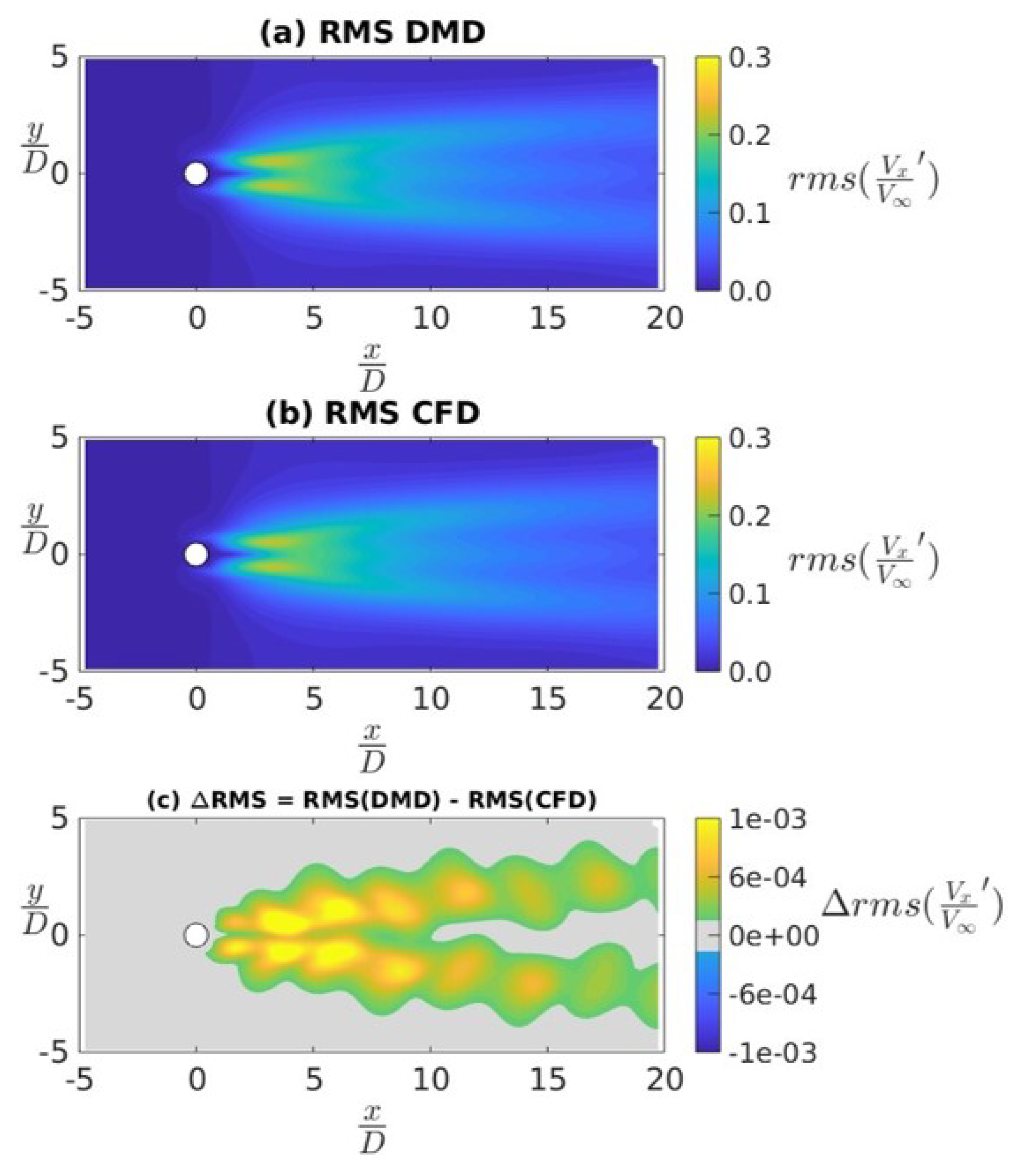
4.2. Application of DMD to a Canonical Flow Case

As a first learning exercise, we performed the DMD of a canonical flow past a 2D circular cylinder at a Reynolds number of 75, similar to a number of DMD works found in the existing literature [35,36,37]. Figure 2 shows scalars of stream-wise velocity normalized by the freestream velocity at the instant $t^{*}=120$, which is essentially the very last time-step. This very last time instance was chosen for validation as a test case because the DMD predictions from Equation (5), which are in exponential form, are expected (and reported) to diverge with large values of time. As such, the greatest discrepancy between the CFD-predicted and DMD-reconstructed flow fields are more likely to be observed for this time instant. From a comparison of the flow fields as obtained from the DMD reconstruction and the CFD simulation in Figure 2a,b, we can conclude that the DMD reconstruction was qualitatively similar to the CFD prediction. This was an encouraging sign for the ability of the DMD to reconstruct the flow field. Further, in Figure 2c, we plotted the difference in the normalized stream-wise velocity predictions between the DMD reconstruction and CFD simulation. This figure clearly demonstrates that the difference between the DMD-reconstruction and CFD-simulation results for this time instance is very small, with the order of magnitude of the differences being ${10}^{-4}$. Thus, we inferred that the DMD reconstruction of the flow field is very well correlated to the CFD simulation results.

However, we note that it is pointless to compare two instantaneous snapshots for turbulent flows. Thus, similar to the Reynolds decomposition approach used in the analysis of turbulent flows, we will be looking at the mean and fluctuating components of the flow field separately. As an example, using the above 2D cylinder case, we present in Figure 3, a comparison of the CFD and DMD results of the normalized mean stream-wise velocity. For both CFD and DMD results, the flow field statistics are taken from the last 30 LETOTs of the simulation data. Similar to the analysis of Figure 2, in Figure 3a,b, we saw that the mean of the DMD reconstructed flow field is qualitatively similar to the one obtained from the CFD simulation. Furthermore, in Figure 3c, we can see that the differences in the mean of the normalized stream-wise velocity prediction between the DMD reconstruction and CFD simulation are very small, $\mathcal{O}\left({10}^{-4}\right)$.

In Figure 4, we see a comparison between the RMS values of normalized stream-wise velocity fluctuations as obtained from the CFD computation and DMD reconstruction. Similar to the previous results, in Figure 4a–c, we see a very negligible difference between the RMS values obtained using the CFD calculations and DMD reconstruction of the flow fields. In Figure 4c, we see that the maximum prediction difference is $\mathcal{O}\left({10}^{-3}\right)$, which is one order larger than the difference seen for the mean component. This indicates that the DMD modes associated with higher frequencies may have more reconstruction error compared to the modes associated with lower frequencies. In subsequent discussions, this frequency-based bias of the DMD-reconstruction error will be explored further using the force and moment time-series data obtained from the Ahmed body CFD simulations.

4.3. Ahmed Body Simulations

The Ahmed body simulation of cases C2 and C3 were run first with a time-step of $\Delta t=0.001\times t^{*}$, which corresponds to a physical time-step of $2.5\times {10}^{-4}$ s, implying a sampling frequency of 4 KHz when data were collected from every time-step. As an initial exploration of the question, “How much data are required to perform an effective DMD?”, we took about $25\%$ of the collected data for the DMD analysis. To address one of the other fundamental questions pertaining to DMD, “What is the necessary sampling frequency for reliable DMD analyses of high-Reynolds-number flows?”, the sampling frequency was increased to 10 kHz, and the necessity and implications of this smaller time-step on the overall veracity of the DMD-reconstruction process will be discussed in later sections.

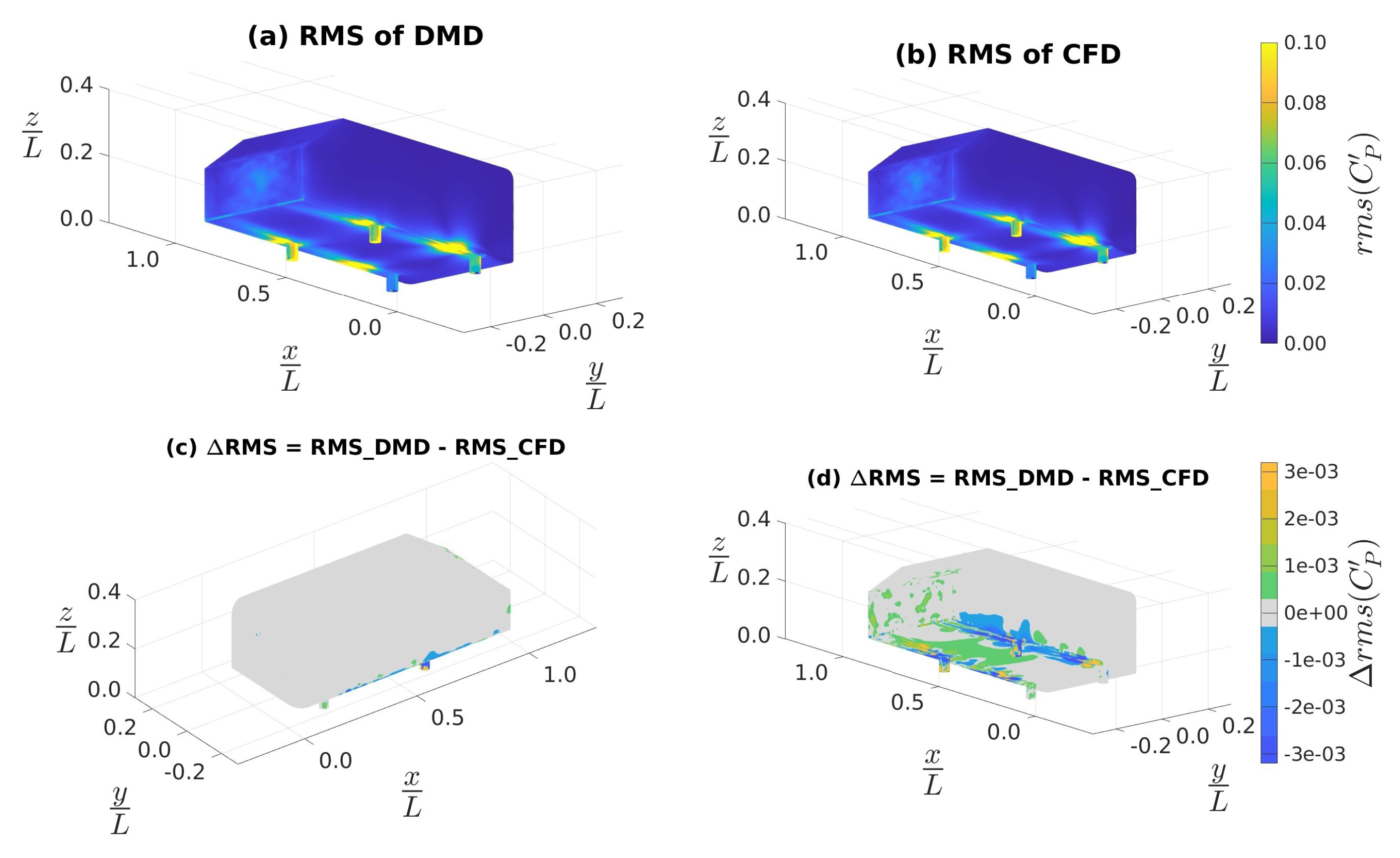
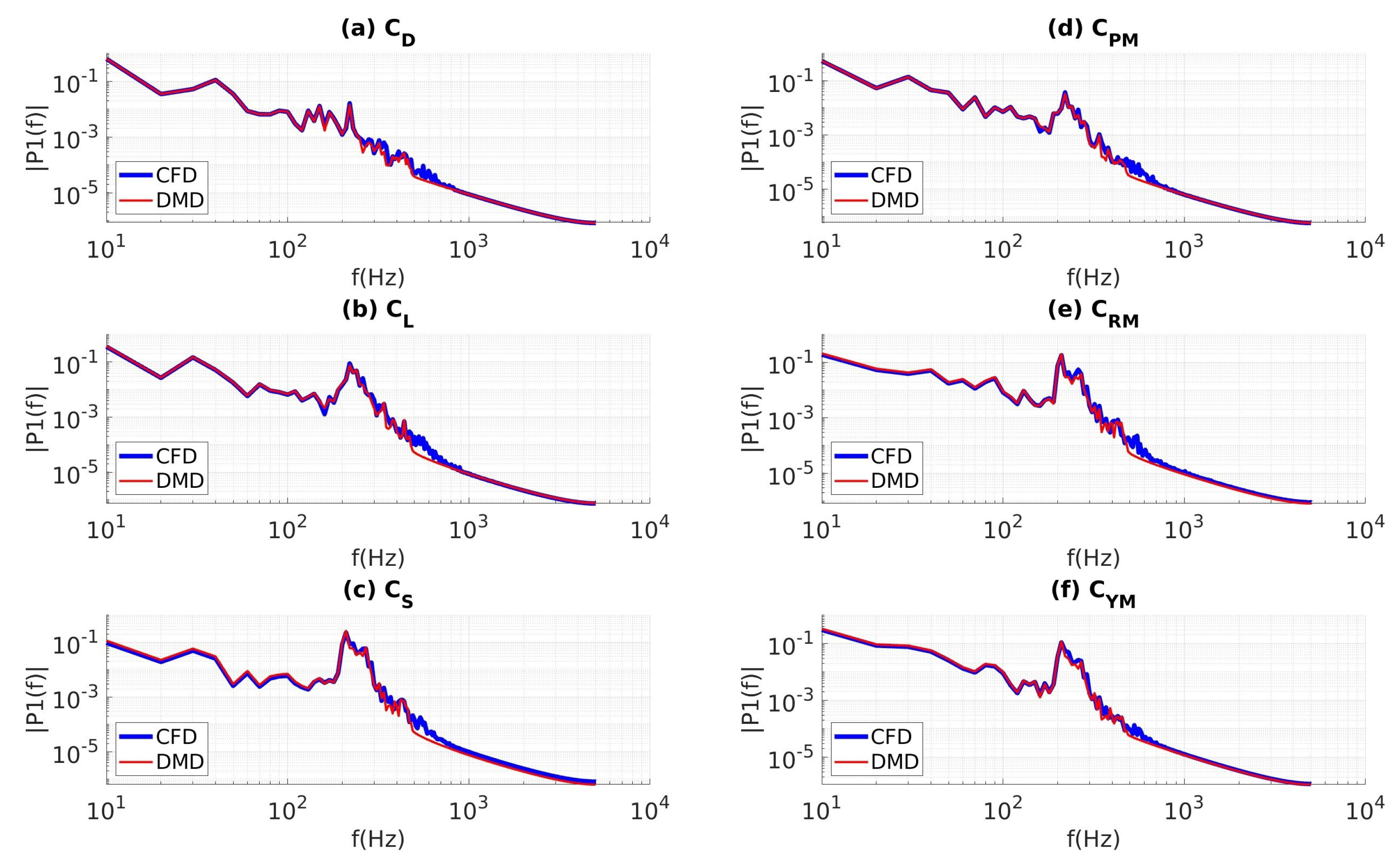
4.3.1. Effectiveness of the DMD Approach Using CFD Data Sampled at 4 kHz

Figure 5a–d show the distribution of mean pressure coefficient $C_P\equiv p/\left(0.5\rho U_{\infty }^2\right)$ on the surface of the Ahmed body; here, p and $U_{\infty }$ represent pressure and reference free-stream velocity, respectively. Note that all sub-figures, unless stated otherwise, are an isometric bottom-right view of the GV. The spatial extents of the coordinate system are non-dimensionalized by the length of the Ahmed body, L. Similar to Figure 3, we see that the distribution of mean $C_p$ on the GV surface is qualitatively the same in both the DMD-reconstruction and CFD-computation results. Note that in subsequent discussions, for simplified references, “results using the DMD-reconstruction” and “results using the actual CFD computations” will be referred to as DMD and CFD results, respectively. Figure 5c,d show the discrepancy in mean $C_p$ prediction by the DMD relative to the CFD results; in Figure 5d, we changed the camera viewing angle to a bottom-right orientation to accommodate visualization of the hidden portions of Figure 5c. In both Figure 5c,d, we noted that the discrepancies were $\mathcal{O}\left({10}^{-3}\right)$. In Figure 5c, we observed that the result differences are mostly toward the rear of the GV and around the edges of the front face. From Figure 5d, we observed that the discrepancies are most pronounced on the rear slant, rear fascia, and around the two downstream stilts, which are regions with recirculation and where smaller vortical structures can exist; see [20,45]. We will revisit this when analyzing Figure 6.

Figure 6a,b show the RMS of surface $C_p$ fluctuations from DMD reconstruction and CFD calculations, respectively. We see a notable discrepancy in the region immediately downstream of the stilts. Figure 6c,d show the discrepancies between the DMD-predicted and CFD-simulated values of the RMS surface $C_p$; note that in Figure 6d, we changed the camera angle to a top-left orientation to accommodate visualization of the hidden portions of Figure 6c. In both Figure 6c,d, we noted that the discrepancies were $\mathcal{O}\left({10}^{-2}\right)$, which is an order of magnitude worse compared to the mean-flow DMD predictions in Figure 5. In addition, in Figure 6d, we observed that the DMD result discrepancy (relative to the CFD results) was due to an underprediction of the fluctuating components along the stilts, rear edges, rear slant and rear face. These were the same regions observed in Figure 5d.

To better quantify the implications of these flow field discrepancies, we integrated the surface static pressure field to obtain the pressure component of force and moment coefficients from both the CFD data and the DMD reconstruction. Figure 7a–f show the time-series data of coefficients of drag, lift, sideforce, and pitching, rolling, and yawing moments, respectively. On each subplot, the CFD simulation data-series is shown in blue, and the DMD reconstruction data-series is shown in red. We can see that DMD reconstruction was able to capture the mean of all the coefficients reasonably well; however, the fluctuating components were seen to exist only in the first $10\%$ of the time-series and then dissipated rapidly thereafter. Even a low-frequency motion in the CFD data was seen to be initially captured by the DMD, but that too dissipated to 5 LETOTS. By investigating the time dynamics component of Equation (5), we found nonphysical growth rates that caused the eventual dissipation of the higher-frequency DMD modes. This is further corroborated by the following frequency analysis.

The Power Spectral Density (PSD) of all six force and moment coefficients obtained using the recorded time-series data are shown in Figure 8a–f. In these figures, PSDs obtained using the actual CFD data and DMD reconstruction of the time-series are shown in blue and red, respectively. It can be seen that all of the DMD spectra were missing many of the characteristic frequencies of the flow. The PSDs obtained form the DMD calculations underpredicted energy contributions form the flow structures in the frequencies from 30 to 300 Hz. Additionally, except for drag, many of the medium-frequency motions from 100–400 Hz are entirely missed for all other components of force and moment in Figure 8b–f. In Figure 8a,b,d, the characteristic PSD peaks around 200 Hz and, amplitude-wise, are significantly underpredicted by the DMD. Thus, we inferred that the present implementation of the DMD process is suffering energy loss due to a nonphysical dampening of medium-to-high-frequency motions.

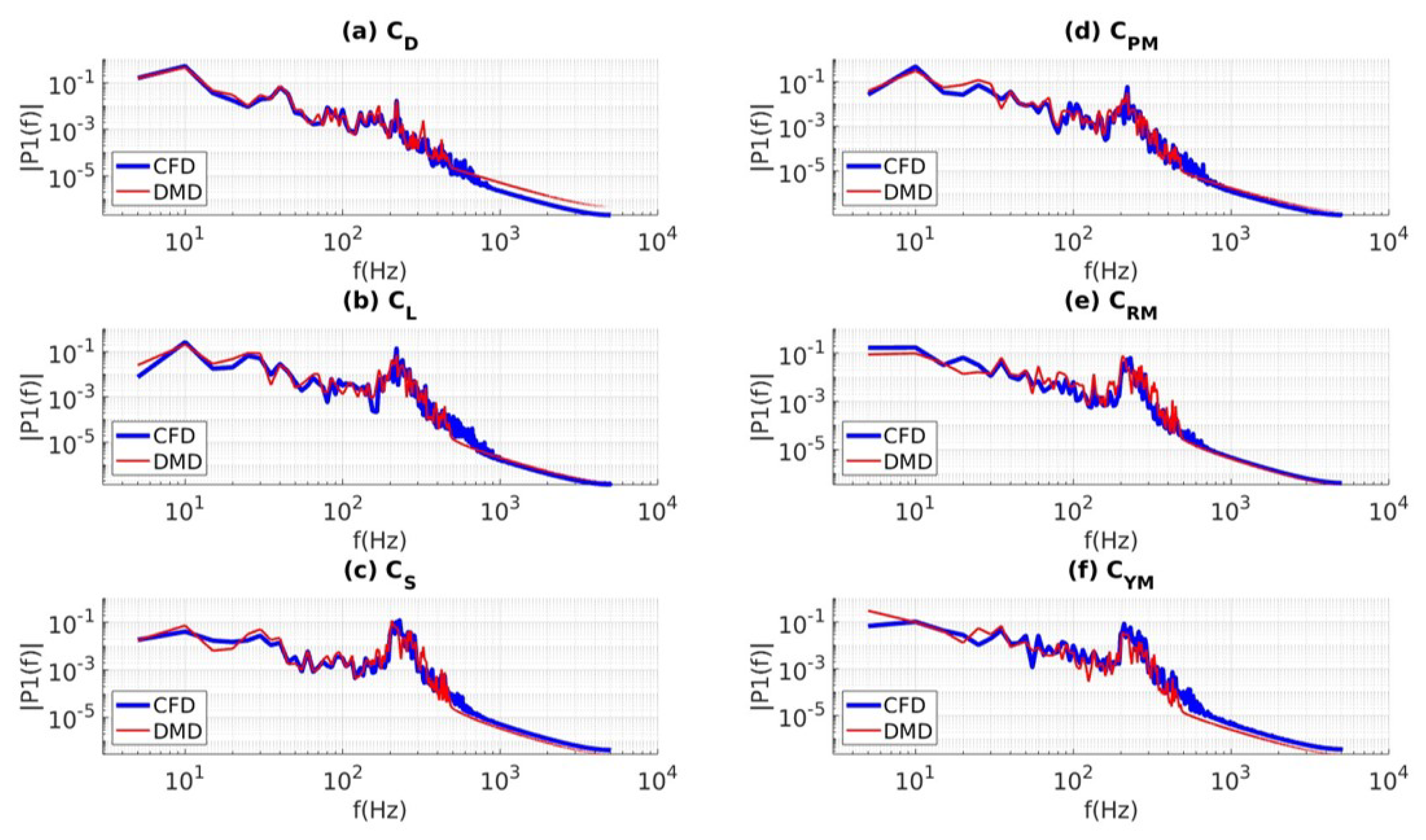
4.3.2. Effectiveness of the DMD Approach Using CFD Data Sampled at 10 kHz

To address one of the fundamental questions pertaining to DMD, “What is the necessary sampling frequency for DMD of high-Reynolds-number flows?”, and to help resolve the issues highlighted in Figure 7 and Figure 8, we increased our sampling frequency to 10 kHz as used by [1] for a much higher Reynolds-number flow. This necessitated a reduction in our CFD time-step size by $60\%$ to $\Delta t=4\times {10}^{-5}{t}^{*}$, a re-run of the CFD simulation, and fresh data collection for DMD at the 10 kHz sampling frequency. To facilitate a consistent comparison of DMD performance between the two CFD runs (using these two different time-steps), the size of the data matrix of Equation (1) was kept constant. Thus, the subsequent plots were generated using about 8 LETOTs of converged CFD data, which represents about 0.2 s of physical time, and a lowest resolved frequency of 4.8 Hz.

Figure 9a,b show the mean $C_p$ distribution on the Ahmed body surface as obtained from the DMD and CFD, respectively, similar to those presented in Figure 5a,b, but determined using data sampled at 10 kHZ. As before (i.e., for the 4 KHz case), we see that the distribution of mean $C_p$ on the GV surface is qualitatively the same in both DMD and CFD. Figure 9c,d show the differences in mean $C_p$ prediction of DMD relative to CFD; in Figure 9d, we changed the camera angle to a bottom-right orientation to help better visualize the hidden portions of Figure 9c. In both of these figures, we noted that the discrepancies were $\mathcal{O}\left({10}^{-4}\right)$, which is an order of magnitude less than that associated with Figure 5c,d, which corresponds to the data sampled at 4 kHz. In Figure 9c, we observed that the discrepancies are nearly eliminated from the upper surface, and the process shows a marked improvement along the edges of the front face, compared to Figure 5c. In Figure 9d, we, however, observed that the discrepancies were still very prominent on the rear slant, the rear fascia, and around the two downstream stilts.

In Figure 10, we observed the distribution of RMS of $C_p$ fluctuations on the surface of the Ahmed body. Figure 10a,b show the RMS of $C_p$ as predicted by DMD and CFD, respectively. In comparison to Figure 6a,b, we see a significant improvement in the region immediately downstream of the stilts. Figure 10c,d show the difference in RMS $C_p$ prediction of DMD relative to CFD; similar to before, in Figure 10d, we changed the camera angle to a top-left orientation to help visualize the hidden portions of Figure 10c. In both Figure 10c,d, we noted that the discrepancies were $\mathcal{O}\left({10}^{-2}\right)$, which was similar to the order of magnitude seen in Figure 6c,d. In Figure 10d, we observed that the discrepancies in DMD are due to underpredictions of the fluctuating components along the stilts, rear edges, rear slant and rear face. These were the same regions highlighted in Figure 6d. Thus, Figure 9 and Figure 10 indicate that the low-to-medium frequency response of DMD improved, but the high frequencies may remain unresolved.

We again integrated the surface static pressure field to get the pressure component of force and moment coefficients from both the CFD simulation and the DMD reconstruction. Figure 11a–f show the time-series data for coefficients of drag, lift, sideforce, and pitching, rolling, and yawing moments, respectively. We can see in Figure 11a–f that the DMD reconstruction was now able to capture the moving mean of all the coefficients, which is a notable improvement from Figure 7a–f. However, in the DMD reconstruction, the higher-frequency fluctuating components are still seen to be dissipated. By investigating the time dynamics component of Equation (5), and plotting the mode amplitudes obtained from Equation (14) vs. their frequency, we found non-physical energies among the higher-frequency DMD modes. This suggested that some of the time dynamics obtained by the DMD reconstruction in Equation (5) involve aspects of frequency, amplitude, and growth rates that are non-physical, which may be due to a consequence of noise in the algorithm. This is further investigated by the following frequency space analysis.

We analyzed the Power Spectral Density (PSD) of all six force and moment coefficient signals in Figure 12a–f; note that the subfigures show the PSD of the coefficients of drag, lift, sideforce, pitching moment, rolling moment, and yawing moment, respectively. Each PSD is plotted on the ordinate, and the frequency on the abscissa. On each subplot, the CFD simulation data-series is shown in blue, and the DMD reconstruction data-series is shown in red. Comparing Figure 8 and Figure 12, we can already tell that, for the medium-frequency range, the performance of the DMD reconstruction is far better when the data are sampled at 10 kHz as opposed to 4 kHz (as used earlier). The high-frequency ranges from 1000 Hz and above are well correlated in Figure 12a,c,e,f, with a minor underprediction in Figure 12b,d. In Figure 12a,b,d,f, we see that the DMD spectra manifested some underprediction in the PSDs for the medium-range frequencies, from 30 to 700 Hz. Within these frequency ranges shown in Figure 12c,e, a good correlation between the DMD reconstruction and the CFD simulation results is evident. At a sampling rate of 10 kHz, flow structures in the frequency range up to 1 kHz can be expected to have reasonably good anti-aliasing. Thus, the medium-frequency energies in the DMD reconstructed flow may still be adversely affected by the noise from the decomposition algorithm. These necessitated us to explore the development of a procedure for the removal of these undesired artifacts from the decomposed modes and time dynamics, which are described in the next section.

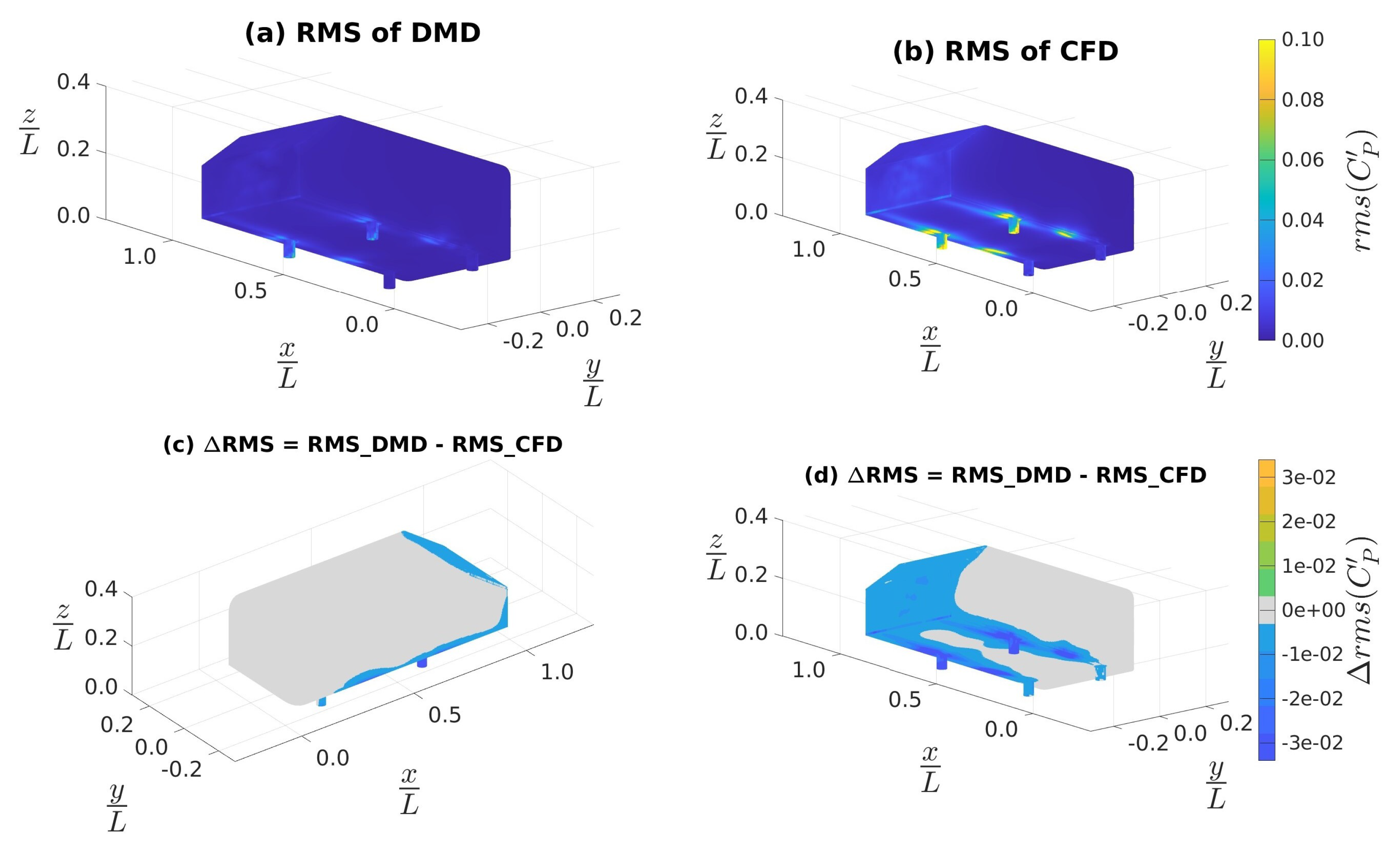
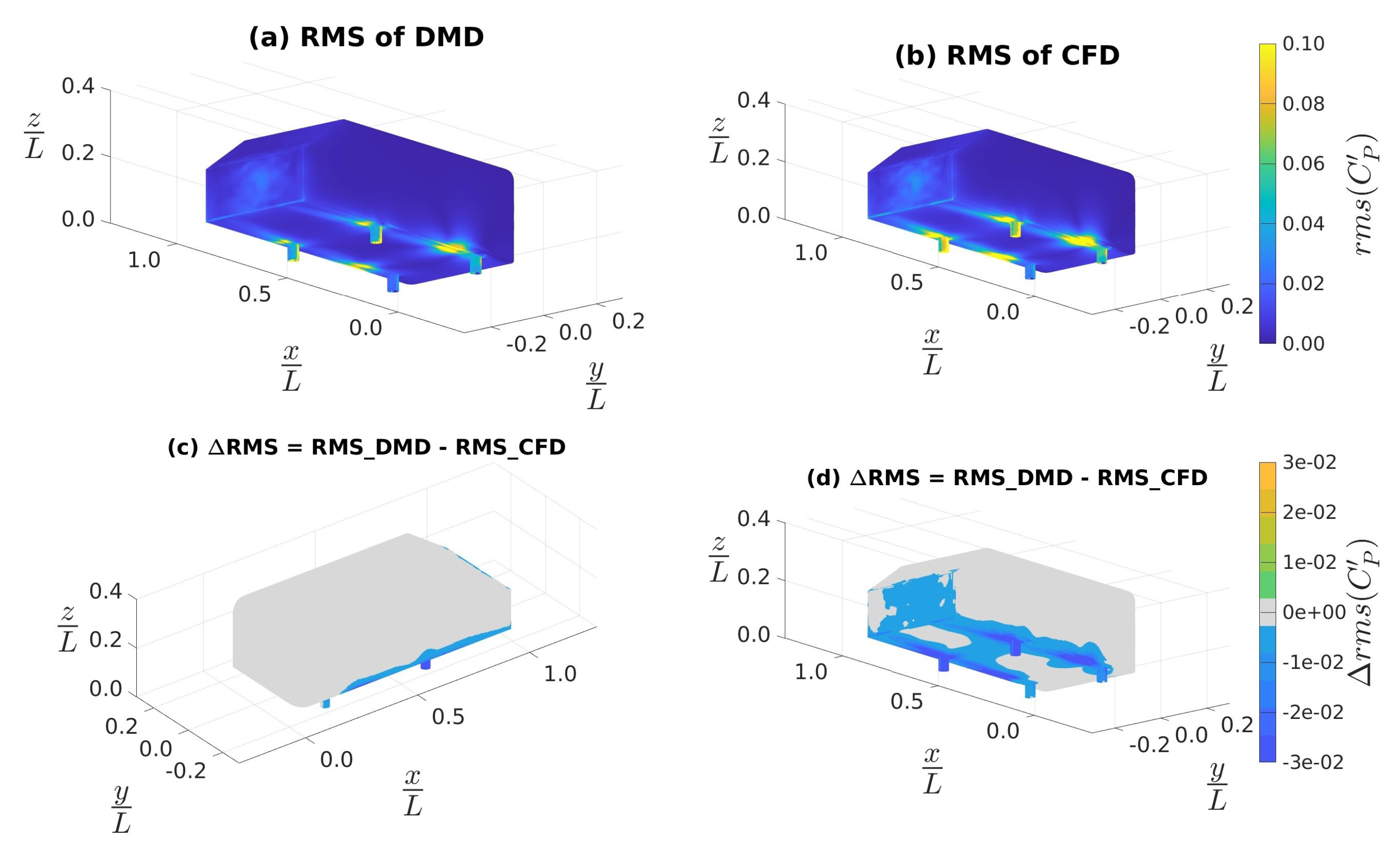
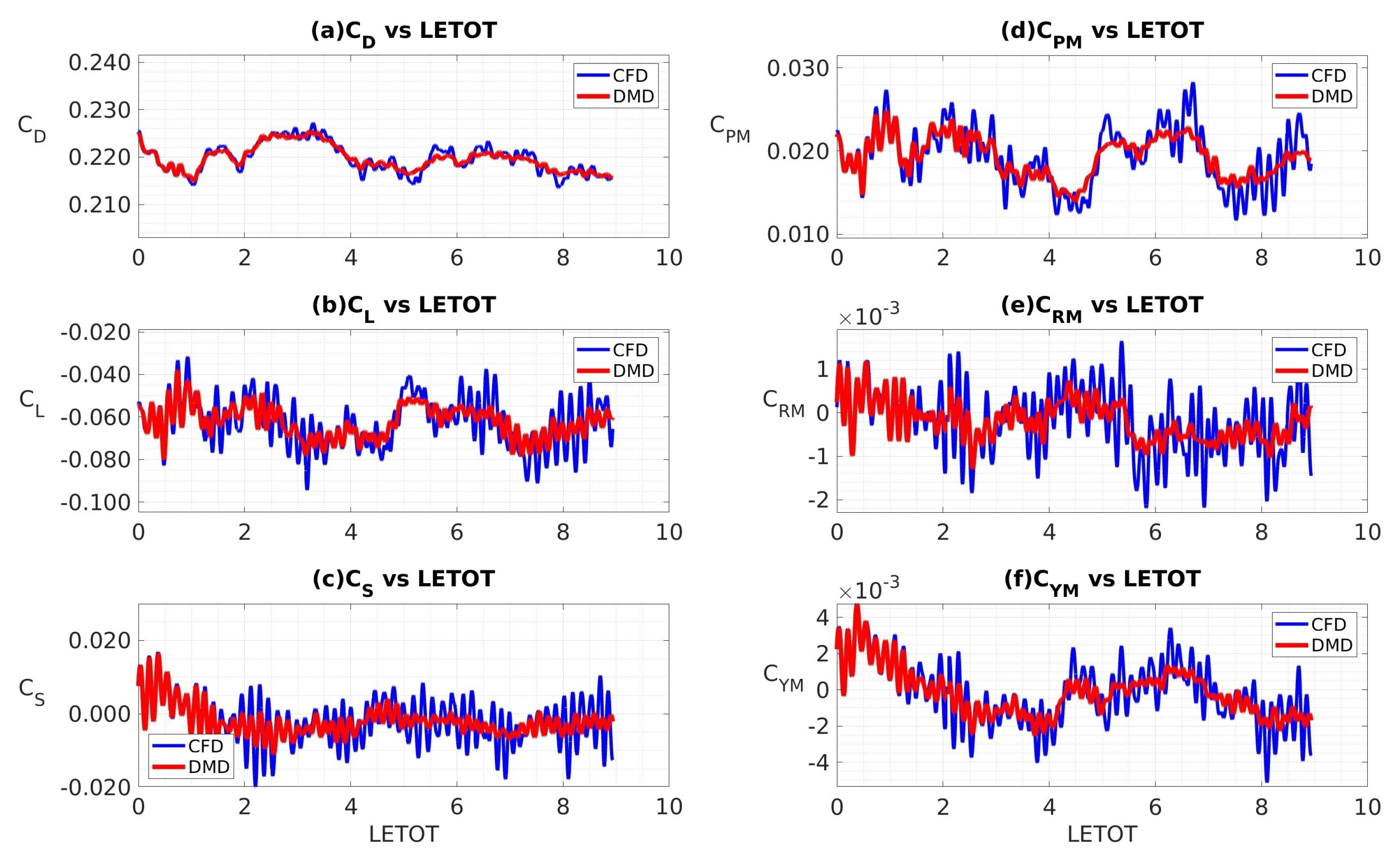
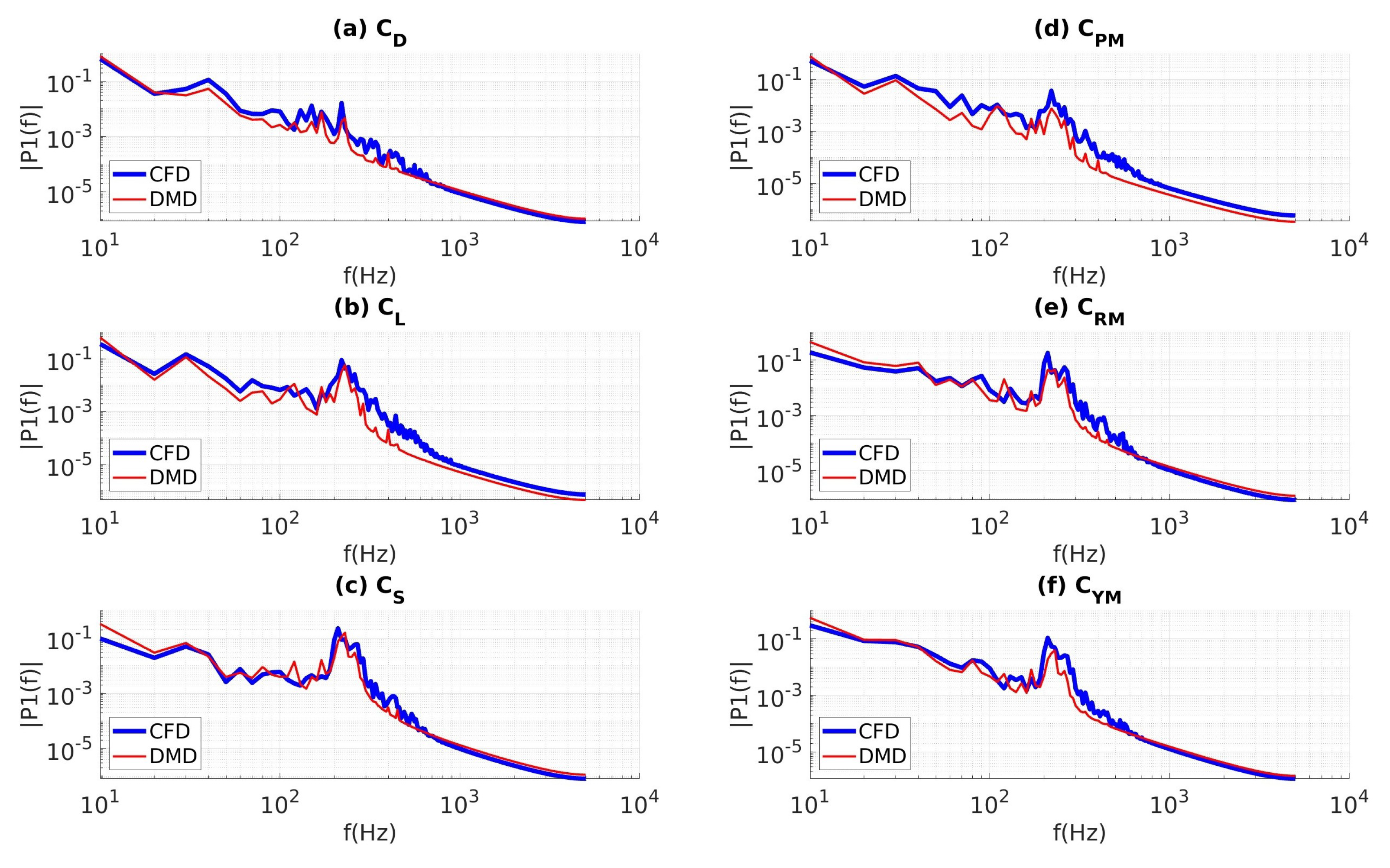
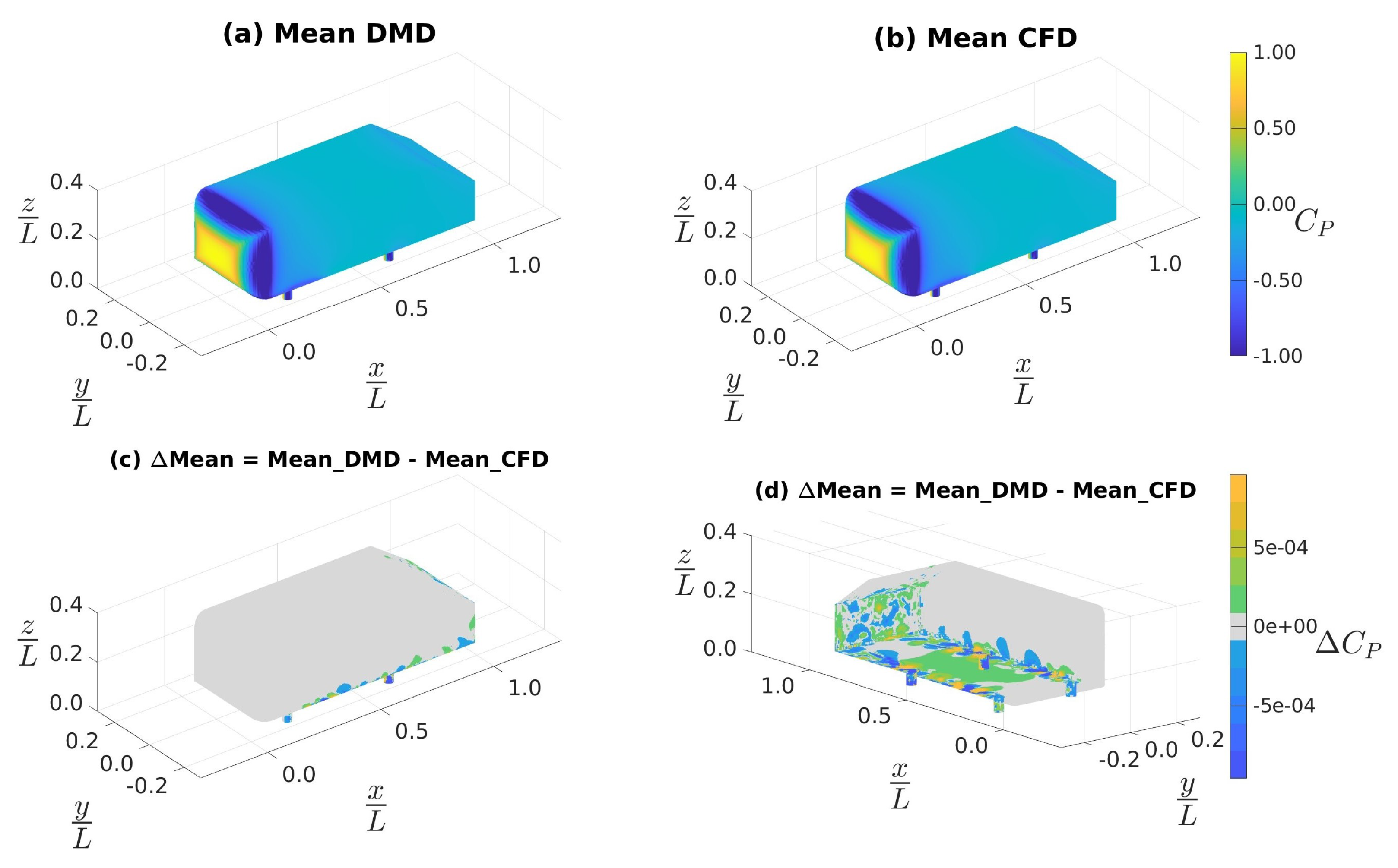
4.3.3. Custom Filtering with Data Sampled at 10 kHz

To circumvent the issues discussed above, we made a modification to the commonly used DMD algorithm. Two changes were made. The first involves the removal of the truncation step of the SVD, and the second involves the introduction of our own custom filtering of the DMD modes. We filtered the time dynamics based on their predicted amplitudes, frequencies and contribution toward the total energy using a series of three sequential filters to identify and remove nonphysical modes. We acknowledge that both the design of the filtration process and the cutoff criteria each require their own methodological optimization, which is left for a subsequent investigation. Here, we briefly describe the filtration process. However, the objective here is to show the concept of filtering out nonphysical modes and how it improved the DMD predictions. After several trials with many strategies and alternatives, we developed a custom filtering approach as described below:

• The first filter was a low-pass filter applied to the modes, identified based on their maximum instantaneous amplitude in the time dynamics term as obtained from Equation (5). The modes with a maximum instantaneous amplitude greater than $50\%$ of the zero-frequency mode were removed.
• The second filter was applied to the modes based on their frequency and their amplitude, given by the RMS version of Equation (14). The second filter was designed to remove high-frequency modes with non-physically excessive energy. To accomplish this, the modes were plotted in frequency space against the amplitudes; among the high-frequency modes ($f>250$ Hz), the spurious modes were identified using a clustering-based anomaly-detection algorithm. Outliers were defined as modes with an amplitude greater than a moving mean of 10 samples by more than a single local standard deviation. The outliers thus identified had their associated modes removed.
• The third filter was designed to remove modes that contribute negligible energy to the system. The remaining modes were sorted based on their contribution toward the total cumulative energy in the system. In this example, modes contributing collectively less than $5\%$ to total energy were removed; we suspect that these modes may arise from the numerical noise. However, this aspect and the effects of the mode cut-off energy limit need to be further investigated.

When this modified DMD process was applied to the 10 kHz sampled data, about 30% of the modes were removed.

Now, let us analyze the same 10 kHz sampled dataset, this time with custom filtering, in the same manner as before. Figure 13a,b show the mean $C_p$ as predicted by DMD reconstruction and CFD prediction, respectively. We see that the distribution of mean $C_p$ on the GV surface is qualitatively the same for both the DMD and CFD results. Figure 9c,d show the discrepancy in the mean $C_p$ prediction of the DMD results relative to the CFD results. In both Figure 13c,d, we noted that the discrepancies were $\mathcal{O}\left({10}^{-4}\right)$, which is the order of magnitude as in Figure 9c,d. However, in Figure 13d, we observed that the errors are nearly absent from the rear slant face, are reduced on the rear face of the GV, and are markedly improved along the edges of the front face—all of which are notable improvements relative to Figure 9d.

Figure 14a,b show the RMS of the fluctuating component of $C_p$ as obtained from the DMD reconstruction and CFD simulations, respectively. In contrast to Figure 10a,b, here the DMD results are virtually identical to the CFD results. Figure 14c,d show the discrepancy in the RMS of the fluctuating component of $C_p$ predicted by DMD reconstruction relative to those predicted by the CFD results; similar to before in Figure 14d, we changed the camera angle to a top-left orientation to visualize the hidden portion of Figure 14c. In both Figure 14c,d, we noted that the discrepancies were $\mathcal{O}\left({10}^{-3}\right)$, which were similar to the order of magnitude seen in Figure 10c,d. This indicates a significant improvement in the prediction of the fluctuating component of the flow field. In Figure 14d, we observed that the discrepancies in the DMD reconstruction are concentrated along the rear edges between the stilts. Thus, Figure 13 and Figure 14 indicate that the medium-frequency response of DMD reconstruction improved through the filtration process. We corroborate this with the subsequent analysis.

We again integrated the surface static pressure field to obtain the pressure component of force and moment coefficients from both the CFD simulation and the DMD reconstruction. Figure 15a–f show a comparison of the time-series data for coefficients of drag, lift, sideforce, pitching moment, rolling moment, and yawing moment, respectively, against the CFD predictions. On each subplot, the CFD simulation data are shown in blue, and the DMD reconstruction data are shown in red. We can see in Figure 15a–f that the DMD reconstruction and CFD simulation predictions are very well correlated, which is a notable improvement from Figure 11a–f. In the DMD reconstruction of Figure 15b,c,e,f, some of the local peaks associated with the CFD simulation are not captured. This could be due to excessive losses in the filtration process and is a subject of our next investigation.

Figure 16a–f show the PSD of coefficients of drag, lift, sideforce, and pitching, rolling, and yawing moments, respectively. Comparing Figure 12 and Figure 16, we can see that the performance of DMD reconstruction using filtered modes, called fmDMD, is better in the medium-frequency range. While there remains some room for improvement within the medium- and high-frequency ranges, we understand that data collected from an IDDES simulation cannot resolve the very high-frequency flow characteristics; in other words, this imitation may be due more to the limitations of the CFD approach and less to the limitations of the DMD approach.

In order to investigate the effectiveness of DMD to predict force and moment coefficients, a comparison of statistical quantities (mean and RMS of the fluctuating component) obtained from the DMD-reconstructed reduced-order flow field against those from the CFD simulations are presented in

Table 1. Mean of all aerodynamic coefficients and RMS of their fluctuations as obtained from the CFD simulation and DMD reconstruction.

	${\mathit{C}}_{\mathit{D}}$	${\mathit{C}}_{\mathit{L}}$	${\mathit{C}}_{\mathit{S}}$	${\mathit{C}}_{\mathit{PM}}$	${\mathit{C}}_{\mathit{RM}}$	${\mathit{C}}_{\mathit{YM}}$
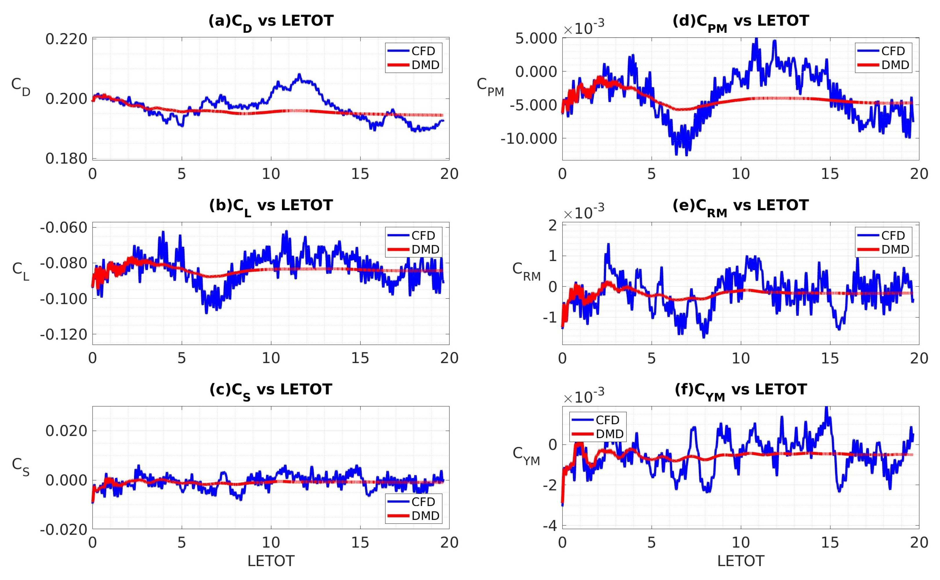
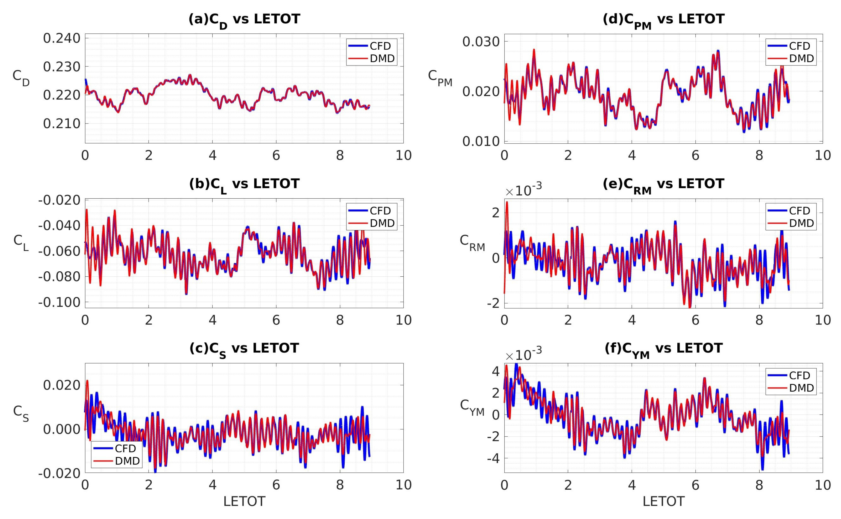
Mean Value from CFD	0.220	−0.062	−0.002	0.019	0.000	0.000
Mean Value from DMD	0.220	−0.062	−0.002	0.019	0.000	0.000
RMS Value from CFD	0.003	0.012	0.006	0.004	0.002	0.001
RMS Value from DMD	0.003	0.012	0.006	0.004	0.001	0.002

. Clearly, the predictions associated with this DMD method (developed in this paper) match very well to the CFD data. Note that the CFD simulation of 2 s of physical time requires 14,400 central processing unit (CPU) hours, where as the DMD averaging over the same period took 15 s of CPU time.

4.4. Future State Predictions Using DMD

We next present the effectiveness of the DMD to make future state predictions of the aerodynamic forces and moments. This was achieved by updating the initial condition vector, $\mathit{b}$, in Equation (5), to represent the last time-step shown in Figure 15. Then, the same coefficients of matrices $\mathbf{\Phi }$ and $\mathbf{\Omega }$ were used in Equation (5) to generate future state predictions of static pressure distribution on the Ahmed body surface. This pressure distribution was then integrated to calculate the aerodynamic forces and moments.

Figure 17a,b show the differences between the future prediction by the DMD relative to the known CFD data (the true value). The instantaneous future predictions by the DMD have small and oscillating differences with reference to the known CFD data. This is expected, as it is unrealistic to expect to perfectly recreate an instantaneous snapshot of a stochastic process, such as the turbulent flow past a ground vehicle. As the existing texts and literature would suggest, for such cases, the parameters of interest are the statistical quantities, such as the mean and RMS of fluctuations and spectral distributions. Thus, we presented a comparison of these time-averaged quantities in

Table 2. Mean of all aerodynamic coefficients and RMS of their fluctuations as obtained from the CFD simulation and future predictions by the DMD-based ROM developed in this study.

	${\mathit{C}}_{\mathit{D}}$	${\mathit{C}}_{\mathit{L}}$	${\mathit{C}}_{\mathit{S}}$	${\mathit{C}}_{\mathit{PM}}$	${\mathit{C}}_{\mathit{RM}}$	${\mathit{C}}_{\mathit{YM}}$
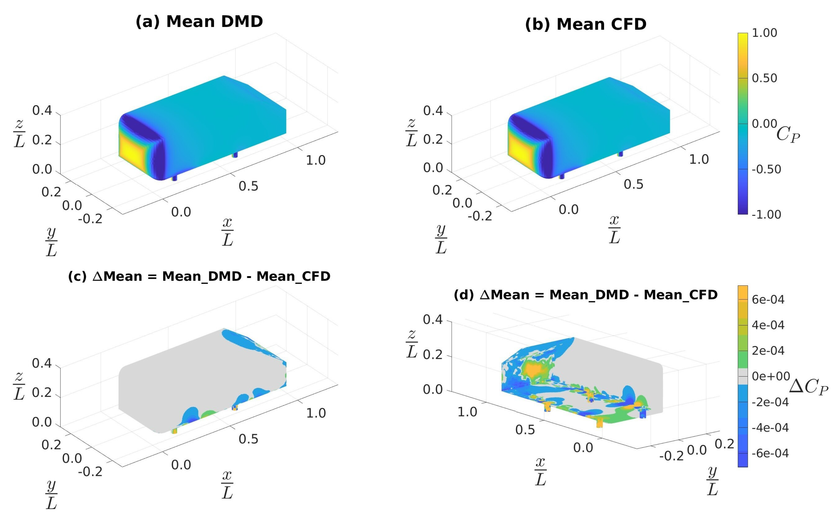
Mean (CFD)	0.220	−0.059	−0.001	0.022	0.000	−0.001
Mean (DMD)	0.218	−0.065	−0.001	0.018	0.000	−0.001
RMS (CFD)	0.002	0.011	0.005	0.003	0.001	0.001
RMS (DMD)	0.001	0.011	0.005	0.003	0.001	0.001

. Generally, the predictions from the DMD method developed in this paper well matched to the CFD data. There is a small discrepancy in the mean CFD and mean DMD coefficients of $C_D,C_L$ and $C_{PM}$ of between two and six counts. This is hypothesized to come from the low-frequency oscillations within the flow field that was not captured in the CFD data used to generate the ROM and is thus not predicted by the DMD. The RMS of the fluctuating components of the DMD and CFD shown in Table 2 are very well matched. This suggests that the proposed ROM successfully predicts the medium- and high-frequency motions.

Figure 18a–f show the PSD of future predictions of the DMD relative to the known CFD data. Similar to Figure 16, spectra of the DMD future prediction are shown in blue, and spectra of the known CFD data are shown in red. Again, the future predictions by DMD are able to capture the PSD of the flow field very well. Small discrepancies are seen in the low-to-medium frequencies in Figure 16e, which indicate that there remains a scope for improvement of the proposed ROM. A sensitivity analysis and optimization are left for future work.

4.5. A Note on Computational Resource Requirements

Finally, in

Table 3. Computational resources required by DMD and CFD.

Parameter	CFD	DMD
Processors	144	1
CPU time for the entire time-series	100 h	<15 s
CPU time for a single time snapshot	5 s	<0.01 s
Storage needed	20 GB	<0.20 GB

, we compare the computational resources required to run the DMD solution shown in Equation (5) against the requirements to run a full-blown CFD simulation. We can see that the DMD is able to reduce the total CPU time and storage requirements by two orders of magnitude. The resources required by DMD are thus expected to be within the capability of an on-board controller on a moving vehicle. The modified DMD process proposed in this paper has the potential to be combined with a control modification, such as the DMD with Control (DMDc) algorithm proposed by [18], and effect real-time control of a moving vehicle. This is a very promising result as a full-blown CFD for real-time control by an on-board computer is not possible.

5. Conclusions

In this paper, we intended to apply the Dynamic Mode Decomposition (DMD) approach to a high-Reynolds-number flow around an idealized ground vehicle with an objective of using the DMD as the engine to develop a Reduced-Order predictive Model (ROM). We observed that the standard DMD algorithm, as available from the existing literature, can successfully reconstruct the low-Reynolds-number flow fields past a 2D cylinder. However, when the same algorithm was applied to a high-Reynolds-number $Re$, separation-dominated complex flow over an idealized ground vehicle, the existing methods failed to accurately reconstruct the flow fields using the derived DMD modes. This implies that a reduced-order reconstruction of the flow field based on the DMD modes obtained using the existing algorithm would be not very reliable for such flows.

It was found that even though a time-step may be sufficiently small for a CFD simulation to resolve the flow field accurately, it may be inadequate to generate a well-resolved dataset required for developing a well-resolved DMD reconstruction methodology. A larger than adequate time-step caused nonphysical growth rates of the modes, which caused excessive energy dissipation of the medium-to-high-frequency modes, which eventually led to total decay of the higher-frequency DMD modes during future-state predictions. Thus, for high $Re$ flows, the data sampling frequency needs to be higher than what may be sufficient on the basis of the time-step size needed for a well-resolved IDDES simulation; this implies that the CFD simulation is needed to be run with a much smaller time-step than necessary for a well-resolved IDDES. Although the higher sampling rate improves the observed discrepancies between the DMD reconstructed values and the ground truth (values from the CFD simulation in this case) for the mean flow variables, the RMS of the fluctuating quantities still shows significant errors. In addition, spectral analyses show that the medium-frequency motions reconstructed by the DMD still show nonphysical dampening. This was hypothesized to be due to the presence of dampening modes emanating from the generation of spurious DMD modes due to the numerical noise present in the CFD training data. Thus, a mode filtration process was developed to remove the offending modes from the DMD reconstruction. This resulted in an order of magnitude improvement in the errors observed in the DMD predictions of the RMS of the fluctuating components when compared to the ground truth. The ROM synthesized via the proposed mode filtration process was able to make a future state prediction that had time-averaged quantities and PSD well correlated to the known CFD data.

The modified DMD reconstruction algorithm presented in this paper was able to overcome the challenges in the medium-to-high-frequency DMD modes. Thus, we demonstrated that the method, called mfDMD, is capable of flow field reconstruction that is correct in the accuracy of the CFD modeling scheme used to generate the training data. The computational resources required by the mfDMD algorithm look feasible for the implementation alongside a DMD with control modification to effect real-time control of a moving vehicle by an on-board controller. Applications of the modified DMD algorithm to aerodynamic interactions between vehicles in close proximity, such as dynamic platooning conditions [45], and NASCAR race cars subject to ride height and crosswind changes [21,51] are the subjects of future research.

References

- Ahani, H.; Nielsen, J.; Uddin, M. The Proper Orthogonal and Dynamic Mode Decomposition of Wake behind a Fastback DrivAer Model; SAE WCX Technical Paper Number 2022-01-0888; SAE International: Warrendale, PA, USA, 2022. [Google Scholar]
- Ikeda, J.; Matsumoto, D.; Tsubokura, M.; Uchida, M.; Hasegawa, T.; Kobayashi, R. Dynamic mode decomposition of flow around a full-scale road vehicle using unsteady CFD. In Proceedings of the 34th AIAA Applied Aerodynamics Conference, Washington, DC, USA, 13–17 June 2016; p. 3727. [Google Scholar]
- Jacuzzi, E.; Granlund, K. Passive flow control for drag reduction in vehicle platoons. J. Wind Eng. Ind. Aerodyn. 2019, 189, 104–117. [Google Scholar] [CrossRef]
- Mohammadikalakoo, B.; Schito, P.; Mani, M. Passive flow control on Ahmed body by rear linking tunnels. J. Wind Eng. Ind. Aerodyn. 2020, 205, 104330. [Google Scholar] [CrossRef]
- Hanfeng, W.; Yu, Z.; Chao, Z.; Xuhui, H. Aerodynamic drag reduction of an Ahmed body based on deflectors. J. Wind Eng. Ind. Aerodyn. 2016, 148, 34–44. [Google Scholar] [CrossRef]
- Siddiqui, N.; Chaab, M. A simple passive device for the drag reduction of an Ahmed body. J. Appl. Fluid Mech. 2020, 14, 147–164. [Google Scholar]
- Tian, J.; Zhang, Y.; Zhu, H.; Xiao, H. Aerodynamic drag reduction and flow control of Ahmed body with flaps. Adv. Mech. Eng. 2017, 9, 1687814017711390. [Google Scholar] [CrossRef]
- Zhang, B.; Liu, K.; Zhou, Y.; To, S.; Tu, J. Active drag reduction of a high-drag Ahmed body based on steady blowing. J. Fluid Mech. 2018, 856, 351–396. [Google Scholar] [CrossRef]
- Joseph, P.; Amandolese, X.; Aider, J.L. Drag reduction on the 25° slant angle Ahmed reference body using pulsed jets. Exp. Fluids 2012, 52, 1169–1185. [Google Scholar] [CrossRef]
- Joseph, P.; Amandolese, X.; Edouard, C.; Aider, J.L. Flow control using MEMS pulsed micro-jets on the Ahmed body. Exp. Fluids 2013, 54, 1–12. [Google Scholar] [CrossRef]
- Li, Y.; Cui, W.; Jia, Q.; Li, Q.; Yang, Z.; Morzyński, M.; Noack, B.R. Explorative gradient method for active drag reduction of the fluidic pinball and slanted Ahmed body. J. Fluid Mech. 2022, 932, A7. [Google Scholar] [CrossRef]
- Bruneau, C.H.; Creusé, E.; Depeyras, D.; Gilliéron, P.; Mortazavi, I. Coupling active and passive techniques to control the flow past the square back Ahmed body. Comput. Fluids 2010, 39, 1875–1892. [Google Scholar] [CrossRef]
- Sudin, M.N.; Abdullah, M.A.; Shamsuddin, S.A.; Ramli, F.R.; Tahir, M.M. Review of research on vehicles aerodynamic drag reduction methods. Int. J. Mech. Mechatron. Eng. 2014, 14, 37–47. [Google Scholar]
- Mukut, A.M.I.; Abedin, M.Z. Review on aerodynamic drag reduction of vehicles. Int. J. Eng. Mater. Manuf. 2019, 4, 1–14. [Google Scholar] [CrossRef]
- Bounds, C.P.; Rajasekar, S.; Uddin, M. Development of a Numerical Investigation Framework for Ground Vehicle Platooning. Fluids 2021, 6, 404. [Google Scholar] [CrossRef]
- Zhang, J.; Feng, T.; Yan, F.; Qiao, S.; Wang, X. Analysis and design on intervehicle distance control of autonomous vehicle platoons. ISA Trans. 2020, 100, 446–453. [Google Scholar] [CrossRef]
- Sivanandham, S.; Gajanand, M. Platooning for sustainable freight transportation: An adoptable practice in the near future? Transp. Rev. 2020, 40, 581–606. [Google Scholar] [CrossRef]
- Proctor, J.L.; Brunton, S.L.; Kutz, J.N. Dynamic mode decomposition with control. SIAM J. Appl. Dyn. Syst. 2016, 15, 142–161. [Google Scholar] [CrossRef]
- Tennekes, H.; Lumley, J.L. A First Course in Turbulence; MIT Press: Cambridge, MA, USA, 1972. [Google Scholar]
- Liu, K.; Zhang, B.; Zhang, Y.; Zhou, Y. Flow structure around a low-drag Ahmed body. J. Fluid Mech. 2021, 913, A21. [Google Scholar] [CrossRef]
- Misar, A.S.; Uddin, M.; Pandaleon, T.; Wilson, J. Scale-Resolved and Time-Averaged Simulations of the Flow over a NASCAR Cup Series Racecar; SAE WCX Technical Paper Number 2023-01-0735; SAE International: Warrendale, PA, USA, 2023. [Google Scholar]
- Guilmineau, E.; Deng, G.; Leroyer, A.; Queutey, P.; Visonneau, M.; Wackers, J. Assessment of hybrid RANS-LES formulations for flow simulation around the Ahmed body. Comput. Fluids 2018, 176, 302–319. [Google Scholar] [CrossRef]
- Ashton, N.; West, A.; Lardeau, S.; Revell, A. Assessment of RANS and DES methods for realistic automotive models. Comput. Fluids 2016, 128, 1–15. [Google Scholar] [CrossRef]
- Kutz, J.N.; Brunton, S.L.; Brunton, B.W.; Proctor, J.L. Dynamic Mode Decomposition: Data-Driven Modeling of Complex Systems; SIAM: Philadelphia, PA, USA, 2016. [Google Scholar]
- Schmid, P.J. Dynamic mode decomposition and its variants. Annu. Rev. Fluid Mech. 2022, 54, 225–254. [Google Scholar] [CrossRef]
- Schmidt, O.T.; Colonius, T. Guide to spectral proper orthogonal decomposition. AIAA J. 2020, 58, 1023–1033. [Google Scholar] [CrossRef]
- Muld, T.W.; Efraimsson, G.; Henningson, D.S. Flow structures around a high-speed train extracted using proper orthogonal decomposition and dynamic mode decomposition. Comput. Fluids 2012, 57, 87–97. [Google Scholar] [CrossRef]
- Sieber, M.; Paschereit, C.O.; Oberleithner, K. Spectral proper orthogonal decomposition. J. Fluid Mech. 2016, 792, 798–828. [Google Scholar] [CrossRef]
- Berkooz, G.; Holmes, P.; Lumley, J.L. The proper orthogonal decomposition in the analysis of turbulent flows. Annu. Rev. Fluid Mech. 1993, 25, 539–575. [Google Scholar] [CrossRef]
- Taira, K.; Brunton, S.L.; Dawson, S.T.; Rowley, C.W.; Colonius, T.; McKeon, B.J.; Schmidt, O.T.; Gordeyev, S.; Theofilis, V.; Ukeiley, L.S. Modal analysis of fluid flows: An overview. AIAA J. 2017, 55, 4013–4041. [Google Scholar] [CrossRef]
- Schmid, P.J. Dynamic mode decomposition of numerical and experimental data. J. Fluid Mech. 2010, 656, 5–28. [Google Scholar] [CrossRef]
- Schmid, P.J.; Li, L.; Juniper, M.P.; Pust, O. Applications of the dynamic mode decomposition. Theor. Comput. Fluid Dyn. 2011, 25, 249–259. [Google Scholar] [CrossRef]
- Schmid, P.J.; Violato, D.; Scarano, F. Decomposition of time-resolved tomographic PIV. Exp. Fluids 2012, 52, 1567–1579. [Google Scholar] [CrossRef]
- Wynn, A.; Pearson, D.; Ganapathisubramani, B.; Goulart, P.J. Optimal mode decomposition for unsteady flows. J. Fluid Mech. 2013, 733, 473–503. [Google Scholar] [CrossRef]
- Sakai, M.; Sunada, Y.; Imamura, T.; Rinoie, K. Experimental and numerical flow analysis around circular cylinders using POD and DMD. In Proceedings of the 44th AIAA Fluid Dynamics Conference, Atlanta, GA, USA, 16–20 June 2014; p. 3325. [Google Scholar]
- Hemati, M.S.; Rowley, C.W.; Deem, E.A.; Cattafesta, L.N. De-biasing the dynamic mode decomposition for applied Koopman spectral analysis of noisy datasets. Theor. Comput. Fluid Dyn. 2017, 31, 349–368. [Google Scholar] [CrossRef]
- Erichson, N.B.; Mathelin, L.; Kutz, J.N.; Brunton, S.L. Randomized dynamic mode decomposition. SIAM J. Appl. Dyn. Syst. 2019, 18, 1867–1891. [Google Scholar] [CrossRef]
- Jovanović, M.R.; Schmid, P.J.; Nichols, J.W. Sparsity-promoting dynamic mode decomposition. Phys. Fluids 2014, 26, 024103. [Google Scholar] [CrossRef]
- Guéniat, F.; Mathelin, L.; Pastur, L.R. A dynamic mode decomposition approach for large and arbitrarily sampled systems. Phys. Fluids 2015, 27, 025113. [Google Scholar] [CrossRef]
- Mengmeng, W.; Zhonghua, H.; Han, N.; Wenping, S.; Le Clainche, S.; Ferrer, E. A transition prediction method for flow over airfoils based on high-order dynamic mode decomposition. Chin. J. Aeronaut. 2019, 32, 2408–2421. [Google Scholar]
- Qiu, R.; Huang, R.; Wang, Y.; Huang, C. Dynamic mode decomposition and reconstruction of transient cavitating flows around a Clark-Y hydrofoil. Theor. Appl. Mech. Lett. 2020, 10, 327–332. [Google Scholar] [CrossRef]
- Heft, A.I.; Indinger, T.; Adams, N.A. Experimental and numerical investigation of the DrivAer model. In Fluids Engineering Division Summer Meeting; American Society of Mechanical Engineers: New York, NY, USA, 2012; Volume 44755, pp. 41–51. [Google Scholar]
- Matsumoto, D.; Haag, L.; Indinger, T. Investigation of the unsteady external and underhood airflow of the DrivAer model by dynamic mode decomposition methods. Int. J. Autom. Eng. 2017, 8, 55–62. [Google Scholar] [CrossRef]
- Ahmed, S.R.; Ramm, G.; Faltin, G. Some salient features of the time-averaged ground vehicle wake. SAE Trans. 1984, 93, 473–503. [Google Scholar]
- Uddin, M.; Nichols, S.; Hahn, C.; Misar, A.; Desai, S.; Tison, N.; Korivi, V. Aerodynamics of Landing Maneuvering of an Unmanned Aerial Vehicle in Close Proximity to a Ground Vehicle; SAE Technical Paper 2023-01-0118; SAE International: Warrendale, PA, USA, 2023. [Google Scholar]
- Lienhart, H.; Becker, S. Flow and turbulence structure in the wake of a simplified car model. SAE Trans. 2003, 112, 785–796. [Google Scholar]
- Misar, A. Insight into the Aerodynamics of Race and Idealized Road Vehicles Using Scale-Resolved and Scale-Averaged CFD Simulations. Ph.D. Thesis, The University of North Carolina at Charlotte, Charlotte, NC, USA, 2023. [Google Scholar]
- Dylewsky, D.; Tao, M.; Kutz, J.N. Dynamic mode decomposition for multiscale nonlinear physics. Phys. Rev. E 2019, 99, 063311. [Google Scholar] [CrossRef]
- Tu, J.H. Dynamic Mode Decomposition: Theory and Applications. Ph.D. Thesis, Princeton University, Princeton, NJ, USA, 2013. [Google Scholar]
- Kou, J.; Zhang, W. An improved criterion to select dominant modes from dynamic mode decomposition. Eur. J. Mech. B Fluids 2017, 62, 109–129. [Google Scholar] [CrossRef]
- Misar, A.S.; Uddin, M. Effects of Solver Parameters and Boundary Conditions on RANS CFD Flow Predictions over a Gen-6 NASCAR Racecar; SAE WCX Technical Paper 2022-01-0372; SAE International: Warrendale, PA, USA, 2022. [Google Scholar]
- Shur, M.L.; Spalart, P.R.; Strelets, M.K.; Travin, A.K. A hybrid RANS-LES approach with delayed-DES and wall-modelled LES capabilities. Int. J. Heat Fluid Flow 2008, 29, 1638–1649. [Google Scholar] [CrossRef]
- Gritskevich, M.S.; Garbaruk, A.V.; Schütze, J.; Menter, F.R. Development of DDES and IDDES formulations for the k-ω shear stress transport model. Flow Turbul. Combust. 2012, 88, 431. [Google Scholar] [CrossRef]
- Spalart, P.R. Comments on the Feasibility of LES for Wings and on the Hybrid RANS/LES Approach. In Proceedings of the First AFOSR International Conference on DNS/LES, Ruston, LA, USA, 4–8 August 1997; pp. 137–147. [Google Scholar]
- Spalart, P.R.; Streett, C. Young-Person’s Guide to Detached-Eddy Simulation Grids; 21076-1320; NASA STI Help Desk, NASA Center for AeroSpace Information: Hanover, MD, USA, 2001.
- Spalart, P.R.; Deck, S.; Shur, M.L.; Squires, K.D.; Strelets, M.K.; Travin, A. A new version of detached-eddy simulation, resistant to ambiguous grid densities. Theor. Comput. Fluid Dyn. 2006, 20, 181–195. [Google Scholar] [CrossRef]
- Piomelli, U.; Balaras, E. Wall-layer models for large-eddy simulations. Annu. Rev. Fluid Mech. 2002, 34, 349–374. [Google Scholar] [CrossRef]
- Menter, F.R. Two-equation eddy-viscosity turbulence models for engineering applications. AIAA J. 1994, 32, 1598–1605. [Google Scholar] [CrossRef]
- Menter, F. Zonal two equation kω turbulence models for aerodynamic flows. In Proceedings of the 23rd Fluid Dynamics, Plasmadynamics, and Lasers Conference, Orlando, FL, USA, 6–9 July 1993; p. 2906. [Google Scholar]
- Menter, F.R.; Kuntz, M.; Langtry, R. Ten years of industrial experience with the SST turbulence model. Turbul. Heat Mass Transf. 2003, 4, 625–632. [Google Scholar]
- Zhang, C.; Bounds, C.P.; Foster, L.; Uddin, M. Turbulence modeling effects on the CFD predictions of flow over a detailed full-scale sedan vehicle. Fluids 2019, 4, 148. [Google Scholar] [CrossRef]
- Aultman, M.; Wang, Z.; Duan, L. Effect of time-step size on flow around generic car models. J. Wind Eng. Ind. Aerodyn. 2021, 219, 104764. [Google Scholar] [CrossRef]
- Misar, A.S.; Bounds, C.; Ahani, H.; Zafar, M.U.; Uddin, M. On the Effects of Parallelization on the Flow Prediction around a Fastback DrivAer Model at Different Attitudes; SAE WCX Technical Paper 2021-01-0965; SAE International: Warrendale, PA, USA, 2021. [Google Scholar]
- Daily, J.W.; James, W.; Harleman, D.R. Fluid Dynamics; Addison-Wesley: London, UK, 1966. [Google Scholar]
- Fu, C.; Bounds, C.P.; Selent, C.; Uddin, M. Turbulence modeling effects on the aerodynamic characterizations of a NASCAR Generation 6 racecar subject to yaw and pitch changes. Proc. Inst. Mech. Eng. Part D J. Autom. Eng. 2019, 233, 3600–3620. [Google Scholar] [CrossRef]
- Hunt, J.C.; Wray, A.A.; Moin, P. Eddies, streams, and convergence zones in turbulent flows. In Studying Turbulence Using Numerical Simulation Databases, 2. Proceedings of the 1988 Summer Program; Center for Turbulence Research: Stanford, CA, USA, 1988. [Google Scholar]
- Fu, C.; Uddin, M.; Zhang, C. Computational Analyses of the Effects of Wind Tunnel Ground Simulation and Blockage Ratio on the Aerodynamic Prediction of Flow over a Passenger Vehicle. Vehicles 2020, 2, 318–341. [Google Scholar] [CrossRef]
- Altinisik, A.; Kutukceken, E.; Umur, H. Experimental and numerical aerodynamic analysis of a passenger car: Influence of the blockage ratio on drag coefficient. J. Fluids Eng. 2015, 137, 081104. [Google Scholar] [CrossRef]