A Hybrid Method to Calculate the Real Driving Range of Electric Vehicles on Intercity Routes

Abstract

A new method to evaluate the energy consumption and driving range of electric vehicles running on intercity routes is proposed. This method consists of a hybridization of a predictive method and the application of online information during the driving run. The method uses specific algorithms for dynamic conditions based on real driving conditions, adapting the calculation method to the characteristics of the route and the driving style; electric vehicle characteristics are also taken into consideration for the driving range calculation. Real data were obtained from driving tests in a real electric vehicle under specific driving conditions and compared with the results generated by a simulation process specifically developed for the new method run under the same operating conditions as the real tests. The comparison showed very good agreement, higher than 99%. This method can be customized according to the electric vehicle characteristics, the type of route and the driving style; therefore, it shows an improvement in the determination of the real driving range for an electric vehicle since it applies real driving conditions instead of protocol statistical data.

1. Introduction

One of the main goals and concerns of today’s electric vehicle manufacturers is the correct estimation of driving range. Although different protocols are available depending on the geographical area (WLTP for the European market [1,2,3,4], FTP-75 and its derivatives for the American one [5,6,7,8], JC08 for the Japanese area [9]), which are used by the manufacturers to predict the driving range of any electric vehicle under specific driving conditions, these protocols are based on statistical analysis of driving tests which, although quite accurate, do not correspond exactly to the driving style of each driver or the specific type of route used or the exact driving conditions. In recent times, different studies have been performed to cover the gap between statistical predictions and real conditions [10,11,12], with the aim of providing manufacturers, designers and drivers a tool to obtain more accurate results in the determination of the real driving range of an electric vehicle [13,14,15,16,17].

Electric vehicle driving range can be obtained either by applying a simulation process based on the use of the associated algorithms [18,19,20,21,22], or from a self-learning process applying real data from previous experiences [23,24,25,26,27,28,29]. This second method, although more accurate, requires a precise knowledge of the driving conditions such as the route characteristics and style of driving, which are not always are available. Furthermore, this method is not entirely predictive since it requires previous information of the route to calculate the driving range [13]. The first method does not require so much deep knowledge of the driving conditions, but the result of the driving range calculation is only estimative. Fuzzy logic is an alternative method that represents a serious contribution in the determination of the driving range of electric vehicles [30]; it allows more or less intensive decision making based on intermediate degrees of compliance with a premise. The accuracy of this method depends on the compliance degree, so if the fulfilment is not high, the prediction can show large divergence from real values.

A hybridization process that uses specific characteristics of the two aforementioned methods could result in a better solution to the problem of calculating the driving range for electric vehicles with maximum accuracy and requiring minimum previous information [31]. Recent studies aimed at this goal have been performed in an attempt to provide the real driving range for electric vehicles and not only an accurate estimation [32]. The solution, however, is far from satisfactory since many variables are involved in the calculation of the real driving range, and many of them are not known previous to the calculation. In this work we propose an improvement in searching for a solution that combines the accuracy of using real data and the application of predictive method calculation.

2. Theoretical Foundations

Driving range in an electric vehicle can be determined using the following expression:

$$DR=\eta \frac{{\xi }_{bat}}{{\zeta }_{rate}}$$

(1)

where ξ_bat represents the energy of the battery in Wh, ζ_rate is the energy consumption rate of the electric vehicle in Wh/km, and η is the efficiency in transferring the energy from the battery to wheels and includes the efficiency of the process of the battery discharge, the performance of the powertrain, and the energy transmission losses.

The energy of the battery can be expressed as a function of voltage and capacity through the equation:

$${\xi }_{bat}=V_{bat}{C}_{bat}$$

(2)

where V is the voltage and C is the capacity.

Nevertheless, the voltage and capacity of batteries in electric vehicles are not constant but time dependent; therefore, Equation (2) should be rewritten as:

$${\xi }_{bat}={\displaystyle \underset{0}{\overset{t_D}{\int }}{V}_{bat}(t)C_{bat}(t)}dt$$

(3)

with t_D being the discharge time.

Since the functions V_bat(t) and C_bat(t) depend on the discharge rate, and this parameter is not constant over the entire discharge, the aforementioned functions adopt different forms depending on the discharge rate; therefore, the integral should be split into as many terms as there are discharge rate values. This solution, although mathematically correct, is not practical and requires a perfect knowledge of the voltage and capacity evolution of the battery as it is being discharged.

A mathematical approximation is the use of a multiple step process replacing the integral function by a summation, which is reasonably accurate if the number of steps is sufficiently large; in such a case, Equation (3) adopts the form:

$${\xi }_{bat}={\displaystyle \sum _{i=1}^n{V}_i{q}_i}$$

(4)

where V_i represents the average value of the battery voltage for the interval i, and q_i is the charge extracted from the battery for the same interval.

Comparing Equations (2) and (4), the following condition must be fulfilled:

$$C_{bat}={\displaystyle \sum _{i=1}^n{q}_i}$$

(5)

In lithium batteries, which are the most currently used in electric vehicles, the voltage decay follows a linear pattern. Thus, the average value can be expressed as:

$$V_i=\frac{V_{o,i}+V_{f,i}}{2}$$

(6)

where V_o,i and V_f,i are the initial and ending value of the battery voltage for the interval i.

The slope of the voltage decay depends on the discharge rate; therefore:

$$V_{f,i}=V_{o,i}-m_i{t}_i$$

(7)

m_i is the slope of the voltage decay for the interval i, and the t_i is the time length of the interval.

Combining Equations (4), (6) and (7), and taking into account that

q_i = I_it_i

(8)

where I_i is the discharge current at the interval i:

$${\xi }_{bat}={\displaystyle \sum _{i=1}^n\left(V_{o,i}-\frac{m_i{t}_i}{2}\right)I_i{t}_i}$$

(9)

The summation of Equation (9) can be extended until the battery is completely discharged. To fulfil this condition, we can express the extracted charge in terms of the battery capacity and calculate the partial depth of discharge corresponding to the ongoing interval; doing so, we obtain:

$${\xi }_{bat}={\displaystyle \sum _{i=1}^n\left(V_{o,i}-\frac{m_i{t}_i}{2}\right)C_r{\left(DOD\right)}_i}$$

(10)

C_r is the real capacity of the battery and (DOD)_i is the partial depth of discharge for the interval i.

Because the battery capacity depends on the discharge rate, it is necessary to introduce a correction factor, f_C, that takes into account the discharge rate dependence. From the literature, we have [33]:

$$f_C=\frac{f_i}{f_{ref}}={\left(\frac{t_i}{t_{ref}}\right)}^{0.0149}={\left(\frac{I_{ref}}{I_i}\right)}^{0.0149}$$

(11)

The term I accounts for discharge, with the sub-index i for the i-step of the process, and ref for the reference process, which currently is referred to 20 h discharge time.

Relating real and nominal capacity, C_n, where the nominal capacity is given by the battery manufacturer, we substitute nominal capacity into Equation (10) and combining this with Equation (11) we have:

$${\xi }_{bat}={\displaystyle \sum _{i=1}^n\left(V_{o,i}-\frac{m_i{t}_i}{2}\right)C_n{f}_C{\left(DOD\right)}_i}={\displaystyle \sum _{i=1}^n\left(V_{o,i}-\frac{m_i{t}_i}{2}\right)C_n{\left(DOD\right)}_i{\left(\frac{I_{ref}}{I_i}\right)}^{0.0149}}$$

(12)

Or:

$${\xi }_{bat}={\displaystyle \sum _{i=1}^n\left(V_{o,i}-\frac{m_i{t}_i}{2}\right)C_n{I}_i{t}_i{\left(\frac{I_{ref}}{I_i}\right)}^{0.0149}=}{\displaystyle \sum _{i=1}^n\left(V_{o,i}-\frac{m_i{t}_i}{2}\right)C_n{t}_i\frac{{\left(I_{ref}\right)}^{0.0149}}{{\left(I_i\right)}^{0.9851}}}$$

(13)

Because the nominal capacity and reference discharge current are constant:

$${\xi }_{bat}=C_n{\left(I_{ref}\right)}^{0.0149}{\displaystyle \sum _{i=1}^n\left(V_{o,i}-\frac{m_i{t}_i}{2}\right)\frac{t_i}{{\left(I_i\right)}^{0.9851}}}$$

(14)

The slope of the voltage decay, m_i, also depends on the discharge rate, as indicated in Equation (15):

$$m_i=\frac{\left(V_C-V_D\right){\left(I_i\right)}^{1.0149}}{C_n{\left(I_{ref}\right)}^{0.0149}}$$

(15)

m_i in Equation (14) is then replaced with Equation (15):

$${\xi }_{bat}=C_n{\left(I_{ref}\right)}^{0.0149}{\displaystyle \sum _{i=1}^n\left[V_{o,i}-\frac{\left(V_C-V_D\right){\left(I_i\right)}^{1.0149}}{C_n{\left(I_{ref}\right)}^{0.0149}}\frac{t_i}{2}\right]\frac{t_i}{{\left(I_i\right)}^{0.9851}}}$$

(16)

V_C and V_D are the battery voltages at full charge and full discharge states.

Equation (16) provides an algorithm that enables the determination of the energy delivered by the battery as a function of the extracted current and time length of every step.

The energy demand indicated in Equation (1), ζ_rate, depends on driving conditions, which, in turn, depend on the route characteristics, driving style and aerodynamic conditions; therefore, when any of the driving conditions change, the energy rate does as well.

Considering an i-interval, as in the previous analysis for the battery performance, the energy demand can be obtained from the power requirements and the time length of the i-interval. Power can be easily determined from the classical expression of the dynamics:

$$P_i=F_i\stackrel{\_\_}{v}$$

(17)

where F_i is the global force acting on the electric vehicle and $\stackrel{\_\_}{v}$ is the average value of the vehicle speed over the entire interval.

The global force is the sum of four contributions: inertial, drag, rolling and potential force. It can be expressed as [31]:

$$F_i=m{a}_i+k{v}_i^2+\mu mg+mg\sin {\alpha }_i$$

(18)

where a is the acceleration, v the vehicle speed, k the drag coefficient, μ the rolling coefficient, α the slope of the road, and m the vehicle mass.

The total amount of energy over the entire route is the sum of partial energies required at every interval; thus:

$${\zeta }_{rate}={\displaystyle \sum _{j=1}^n\left(m{a}_i+k{v}_i^2+\mu mg+mg\sin {\alpha }_i\right)}$$

(19)

Taking into account that the energy requirements and battery delivery should match at every single interval, and extending the analysis over the driving route, we have:

$$DR={\eta }_{pwt}{\displaystyle \sum _{i=1}^n{\left(\frac{{\xi }_{bat}}{{\zeta }_{rate}}\right)}_i=}{\eta }_{pwt}{C}_n{\left(I_{ref}\right)}^{0.0149}{\displaystyle \sum _{i=1}^n\left\{\frac{\left[V_{o,i}-\frac{\left(V_C-V_D\right){\left(I_i\right)}^{1.0149}}{C_n{\left(I_{ref}\right)}^{0.0149}}\frac{t_i}{2}\right]}{\left(m{a}_i+k{v}_i^2+\mu mg+mg\sin {\alpha }_i\right)}\frac{t_i}{{\left(I_i\right)}^{0.9851}}\right\}}$$

(20)

where η_pwt is the powertrain efficiency.

On intercity routes, the driving conditions do not change as often as on urban routes since the driver is not forced to accelerate or reduce speed very often because of traffic. Nevertheless, intercity routes are subject to larger changes in road altitude, which causes a greater influence of the potential term; in addition, the slope of the road is, at many times, high enough to highly influence the driving conditions.

Analyzing Equation (20), we observe that most of the involved terms correspond to set-up values that remain constant over the entire route, including the fully charged and fully discharged battery voltages, the nominal capacity of the battery, the mass of vehicle, and the drag coefficient. As for the rolling coefficient, it can also be considered constant if the type of pavement of the route does not change very much.

The acceleration of an interval, if any, can be expressed as:

$$a_i=\frac{v_{f,i}-v_{o,i}}{t_i}$$

(21)

where v_oi and v_f,i are the initial and final values of the vehicle speed at the i-interval.

The vehicle speed in the drag term is considered as the average value over the i-interval; in cases when the time length of the interval is sufficiently short, the average value can be expressed as:

$$v_i=\frac{v_{f,i}+v_{o,i}}{2}$$

(22)

where a linear variation has been applied.

Replacing acceleration and average speed in Equation (20), the driving range can be expressed as:

$$DR=\eta C_n{\left(I_{ref}\right)}^{0.0149}{\displaystyle \sum _{i=1}^n\left\{\frac{\left[V_{o,i}-\frac{\left(V_C-V_D\right){\left(I_i\right)}^{1.0149}}{C_n{\left(I_{ref}\right)}^{0.0149}}\frac{t_i}{2}\right]}{\left[m\left(\frac{v_{f,i}-v_{o,i}}{t_i}\right)+k{\left(\frac{v_{f,i}+v_{o,i}}{2}\right)}^2+mg\left(\mu +\sin {\alpha }_i\right)\right]}\frac{t_i}{{\left(I_i\right)}^{0.9851}}\right\}}$$

(23)

The variable terms in Equation (23) along the route can be obtained from the corresponding sensors that installed on the electric vehicle, including the speedometer, inclinometer, battery voltmeter and ammeter, and clock time counter. The other parameters involved in Equation (23) are fixed and can be obtained from a data base.

3. Methodological Procedure

The hybrid methodology consists of a combination of a predictive method and an online verification. The predictive method uses the route characteristics and expected driving conditions to estimate the driving range over a specific intercity route, and the online verification applies measurement data from the electric vehicle sensors to correct the predictions. Equation (23) can be used at any time to determine the driving range from the dynamic driving conditions, route characteristics and vehicle specifications.

The implemented software in the electric vehicle control unit (EVCU) makes the corresponding calculations using Equation (23) and data provided through a simulation process that is carried out before starting up [13]. The simulation uses the route profile provided by any of the GPS applications installed in modern vehicle navigators (Google Maps, Sygic, Petal Maps, Geo Track, etc.) and divides the route path into small segments of short duration, generally 1 s, in order to satisfy the established boundary conditions to be able to use Equation (23) to its full extent. The minimum vehicle speed to match the aforementioned GPS resolution and time interval is 18 km/h, which is far below the current speed in intercity routes; therefore, it can be ensured that the positioning of the vehicle is obtained with sufficient precision at every time interval.

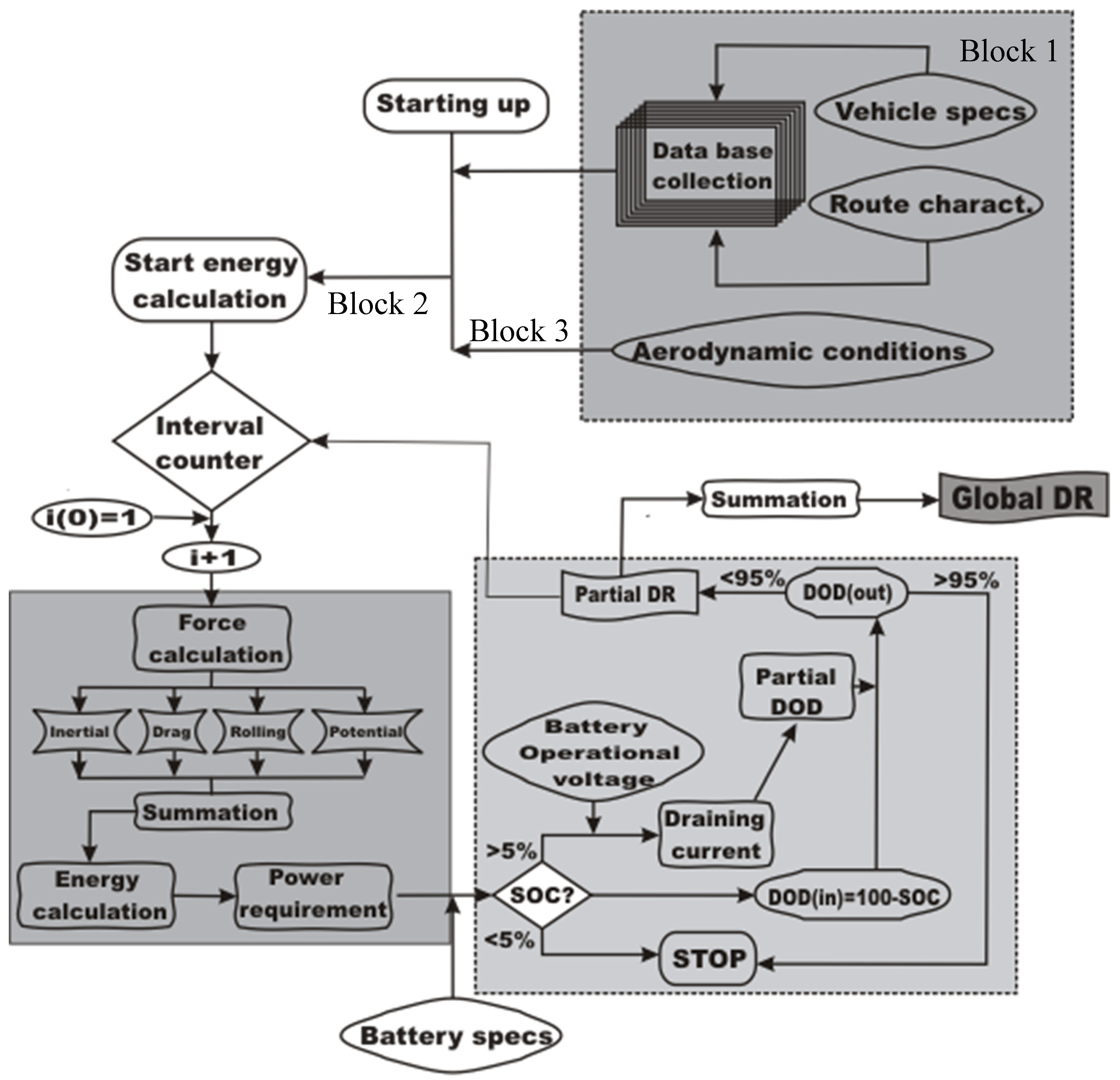
The specific software has been developed following a block structure as represented in Figure 1. The first block corresponds to a subroutine that introduces specific data from the data base related to the characteristics of the route, the electric vehicle specifications, and the aerodynamic conditions. These data correspond to fixed parameters in Equation (23), including the mass of the vehicle, its aerodynamic coefficient, and the rolling and drag coefficients. The second block corresponds to the subroutine that calculates the mechanical force at every interval to obtain the power and energy requirements to maintain the specified driving conditions. Finally, the third block deals with the performance of the battery, determining the current and energy extracted as well as the state of charge (SOC) or depth of discharge (DOD) after completing every interval, thus obtaining the accumulated depth of discharge. The subroutine of this block determines the partial driving range associated with every time interval and the cumulative driving range over the number of intervals until the DOD parameter reaches the set-up value for the minimum state of charge.

Intercity Route Model

To evaluate the driving range from a predictive mode, an intercity route model was designed; the route consists of a series of flat terrain, ascent and descent segments as outlined in

Table 1. Distribution of the travelled distances grouped by type of segment.

Type of Segment	Flat Terrain	Ascent	Descent
Distance (m)	3569.96	5476.15	3376.70
Average slope (°)	0	1.19	−1.84

.

The values shown in Table 1 correspond to the cumulative distances for flat terrain, ascent and descent segments, respectively, of the entire route. All segments included in each category (flat terrain, ascent or descent) have identical characteristics; thus, they can be grouped in a single category with its representative travelled distance. The slope of the route for the ascent and descent category is the result of averaging the slope of the different included segments.

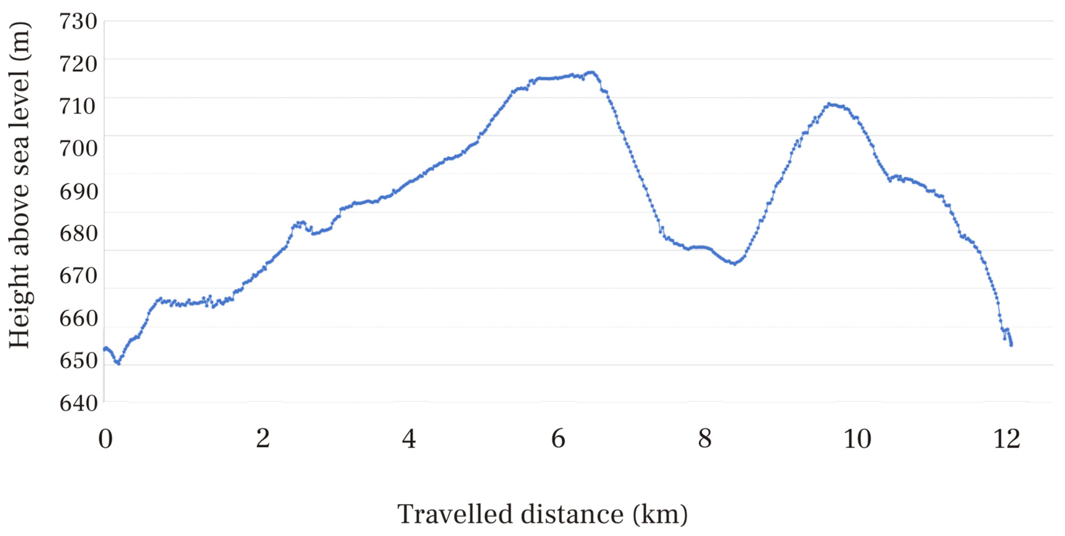
The schematic representation of the intercity route model is the result of modelling a real intercity route, which is used as a testing bench for the validation of the proposed predictive model. The real route configuration is represented in Figure 2, where the route profile has been obtained from satellite data using a GPS application.

Table 2. Orographic characteristics of the real intercity route.

Segment	1	2	3	4	5	6	7
Travelled distance (m)	25.57	173.61	645.84	845.25	1035.01	220.05	367.05
Slope (°)	1.11	−1.34	1.33	0.00	1.10	−0.63	0.96
Segment	8	9	10	11	12	13	14
Travelled distance (m)	434.86	1336.28	777.97	815.01	1054.19	586.60	320.18
Slope (°)	0.21	0.62	1.19	0.20	−2.34	−0.25	−0.57
Segment	15	16	17	18	19	20
Travelled distance (m)	1288.42	271.17	522.17	296.91	816.28	590.41
Slope (°)	1.25	−0.28	−1.77	−0.02	−1.08	−2.67

shows the orographic characteristics of the real intercity route used as a testing bench. It can be observed that the route has been divided into twenty segments, considering the slope of the route as the key parameter for the segment definition; a sudden change in the road slope defines the ending limit of a segment and the initial limit of the next one.

The ascent road group includes segments with slope equal to or higher than 1°, and descent road group corresponds to segments with slope equal to or lower than −1°; any other segments, with slope between −1° and +1° have been included in the flat terrain group.

The average slope of every group has been determined using the following expression:

$$\stackrel{\_\_}{\alpha }=\frac{{\displaystyle \sum _i{L}_i{\alpha }_i}}{{\displaystyle \sum _i{L}_i}}$$

(24)

where L_i and α_i are the travelled distance and the slope of the segment, respectively.

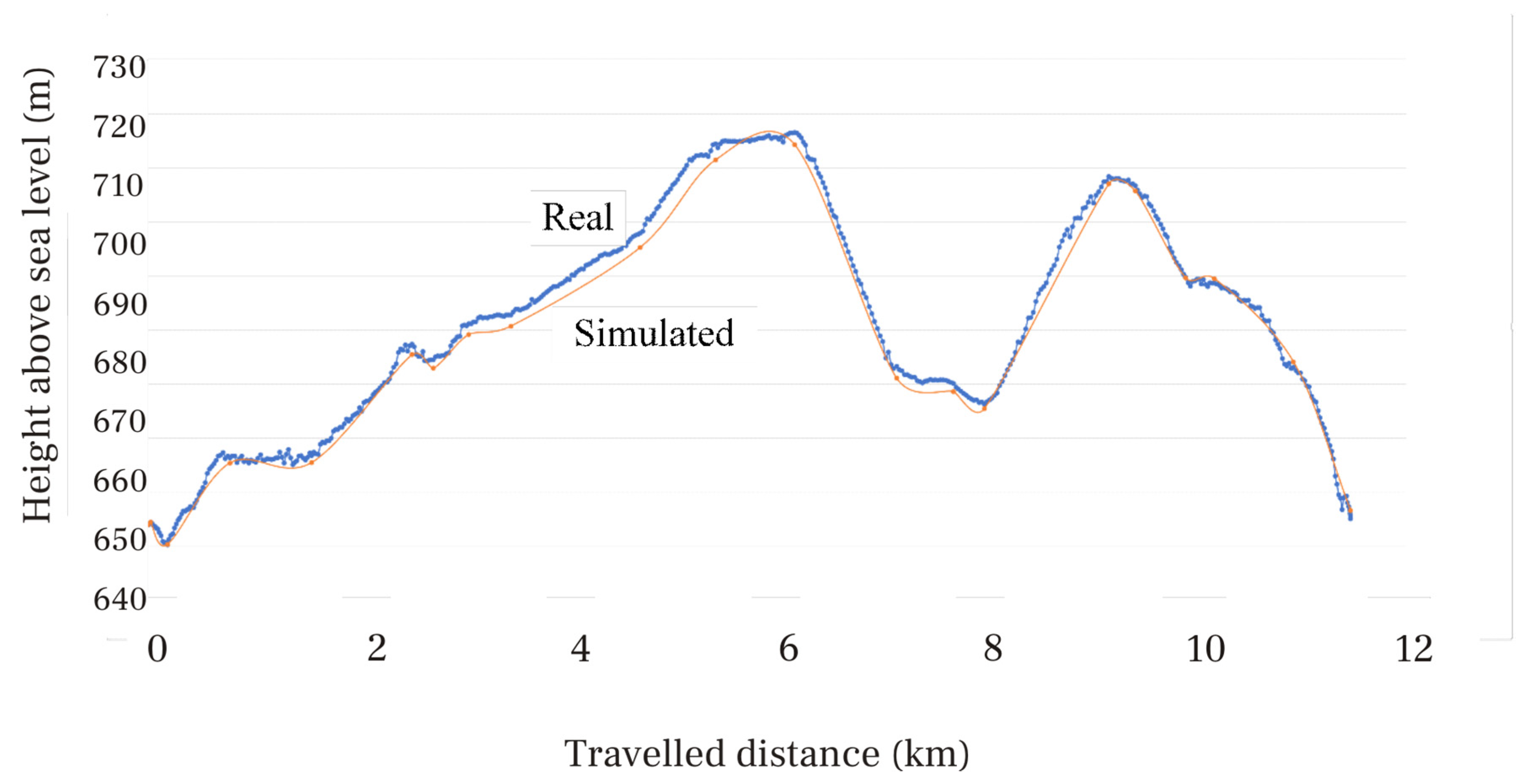
A simulation process was run to reproduce the profile of the real intercity route using the slope of the road as a key parameter, and the results can be seen in Figure 3.

It can be observed that there is excellent agreement between theoretical (simulated) and real profile of the intercity route, proving that the simulation process is highly accurate.

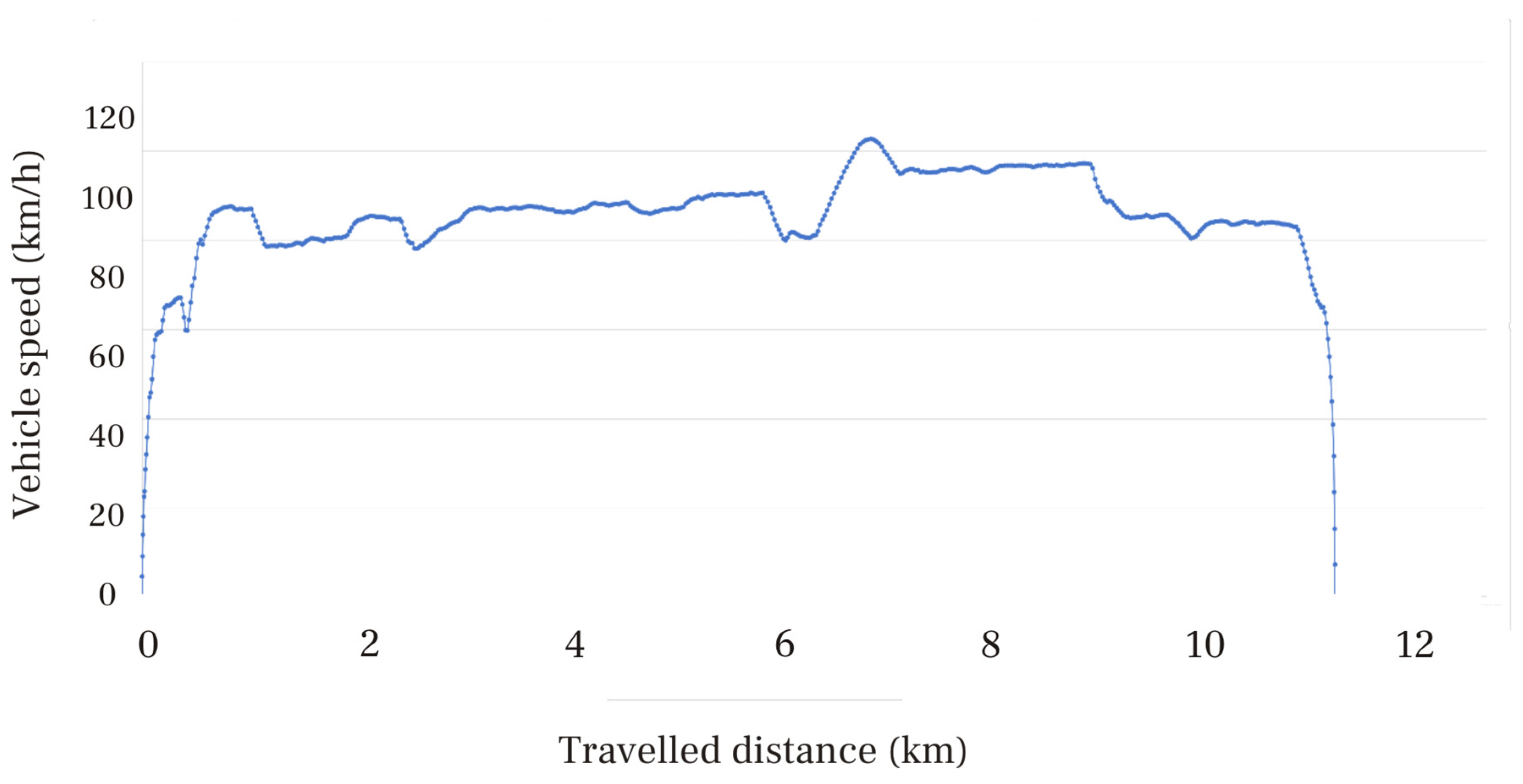
The simulation was extended to the elaboration of the vehicle speed and acceleration profile, which can be seen in Figure 4 and Figure 5, respectively.

Looking at the speed profile of Figure 4, we realize there is a rather constant speed of the electric vehicle over the entire route, which is in good agreement with the set-up statement of short acceleration periods and longer distances at constant speed that was the basis of the calculation process.

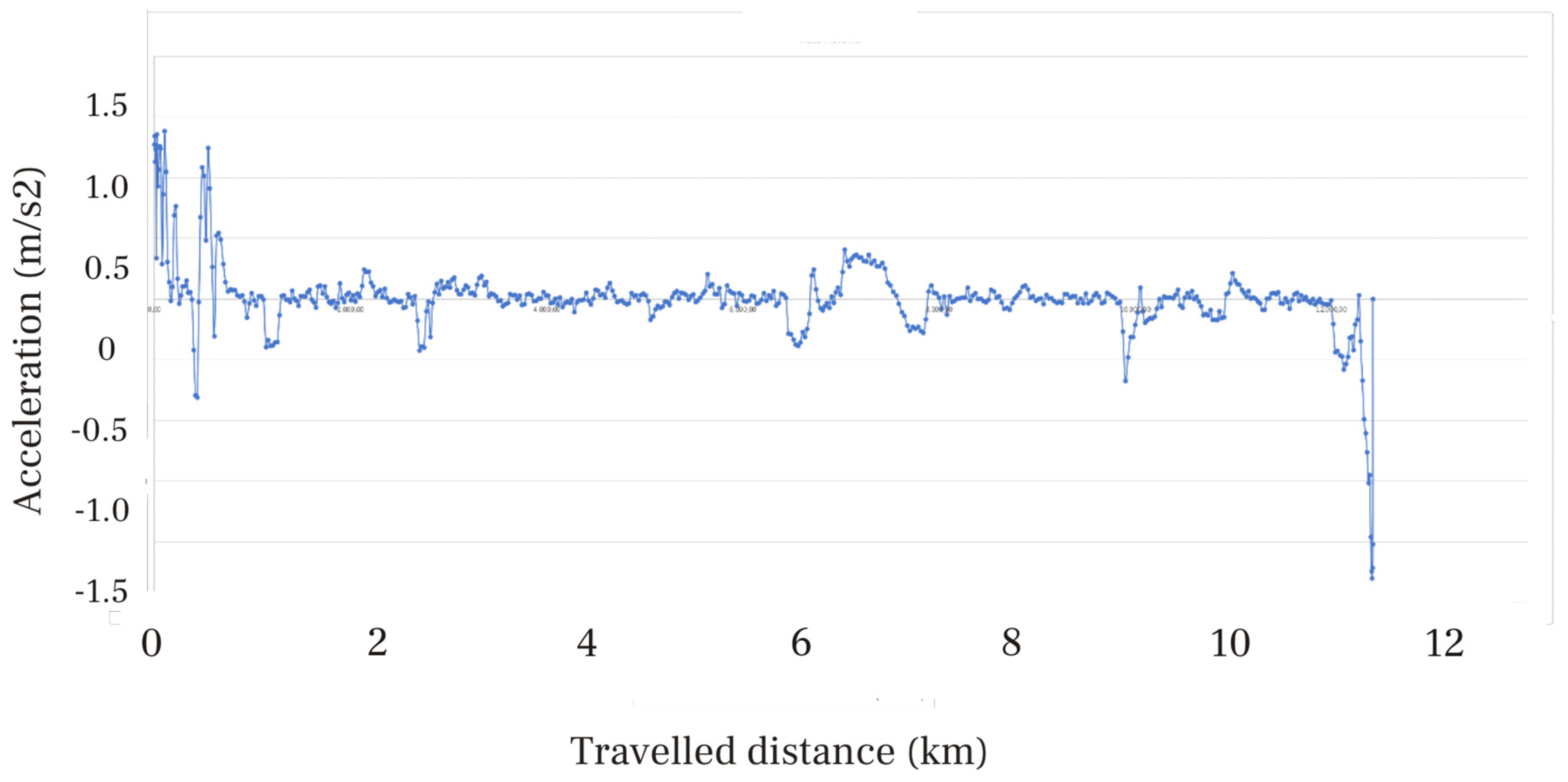
The acceleration profile of Figure 5 shows a near null value over a large fraction of the route with significant variations at the beginning and end of the route that correspond to the starting up and stopping period. The profile of Figure 5 also shows slight variations in the acceleration value due to changes in road level (smallest variations) or the need to accelerate to pass other vehicles (intermediate variations).

The last section of the predictive method calculates the global force required to maintain the driving conditions through the use of Equation (18), resulting in the following graph evolution (Figure 6).

Once the global force has been determined, the predictive method calculates the energy consumption by applying the classical expression:

$$\xi ={\displaystyle \sum _{i=1}^n{F}_i\stackrel{\_\_}{v_i}\Delta t_i}$$

(25)

where F_i corresponds to the global force of every interval of the route, $\stackrel{\_\_}{v_i}$ is the average value of the vehicle speed at this interval, and Δt_i is the time length of the interval.

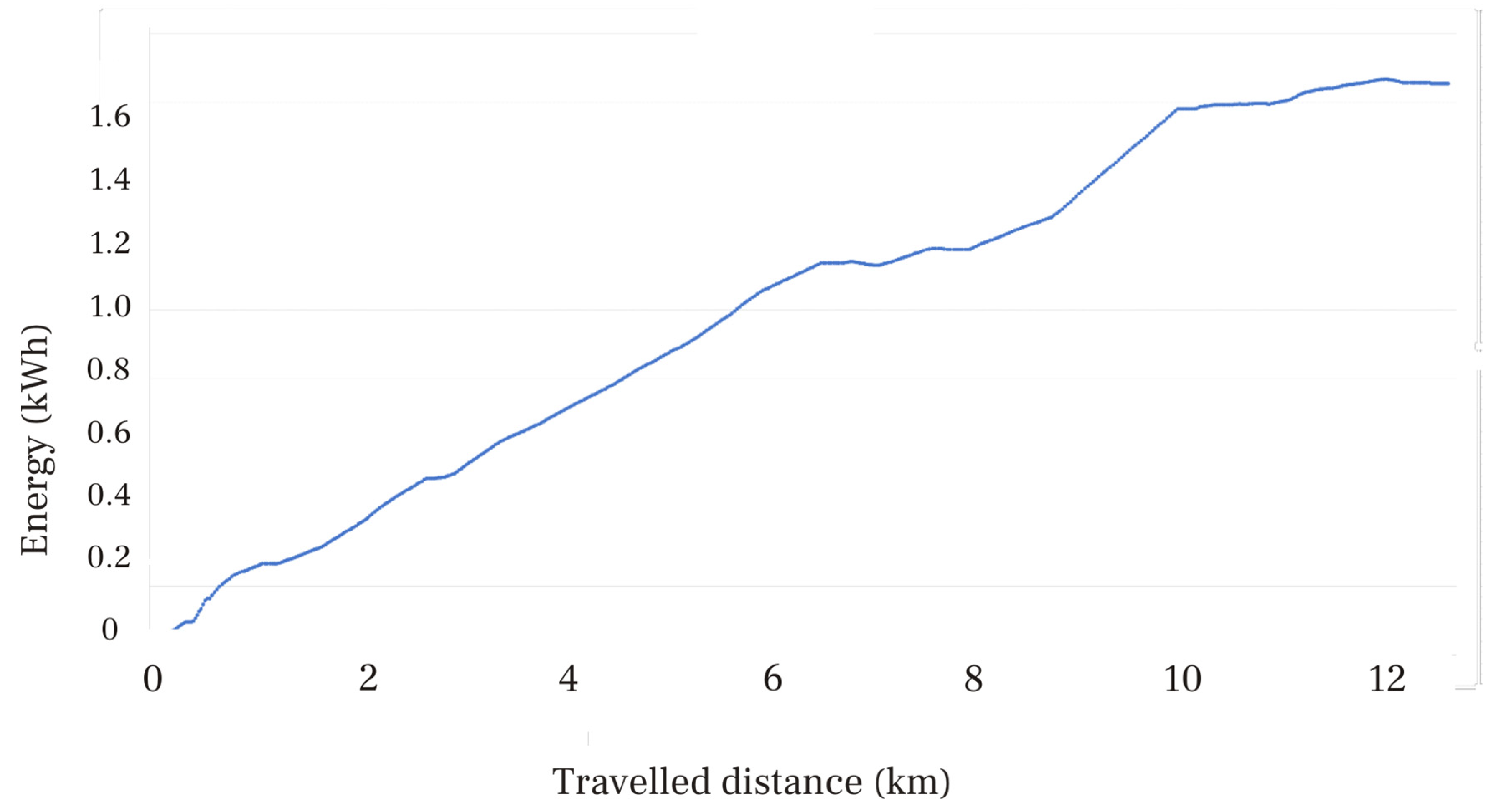
Figure 7 shows the graph of the predicted energy consumption with travelled distance, with an average consumption rate of 133.1 Wh/km, which is in the range of a utility electric vehicle that is the model used for simulation.

Once the predictive method evaluated the power and energy consumption of the set-up intercity route under specific driving conditions, the online method was applied. This online method consists of verifying the estimated results from the predictive method for the power and energy at every time interval. To do so, the electric vehicle is equipped with specific sensors to determine the values of the critical parameters for the online method, such as battery voltage and draining current, travelled distance, slope of the road, vehicle speed, and elapsed time.

The online method uses a very short time interval, currently 1 s, to obtain real values of power and energy delivered by the battery. The energy extracted from the battery is calculated from the electric parameters and time lapse, using the expression:

$${\xi }_{bat}={\displaystyle \sum _{i=1}^n{I}_i{V}_i\Delta t_i}$$

(26)

where I_i and V_i are the average values of current and voltage of the battery, respectively, during the set-up time interval, and ∆t_i is the time interval (1 s).

Applying Equations (16) and (19), and considering that the energy demand of the electric vehicle and energy extracted from the battery are related through the powertrain efficiency, the energy extracted from the battery is calculated as:

$${\xi }_{bat}=\frac{{\zeta }_{rate}}{{\eta }_{pwt}}$$

(27)

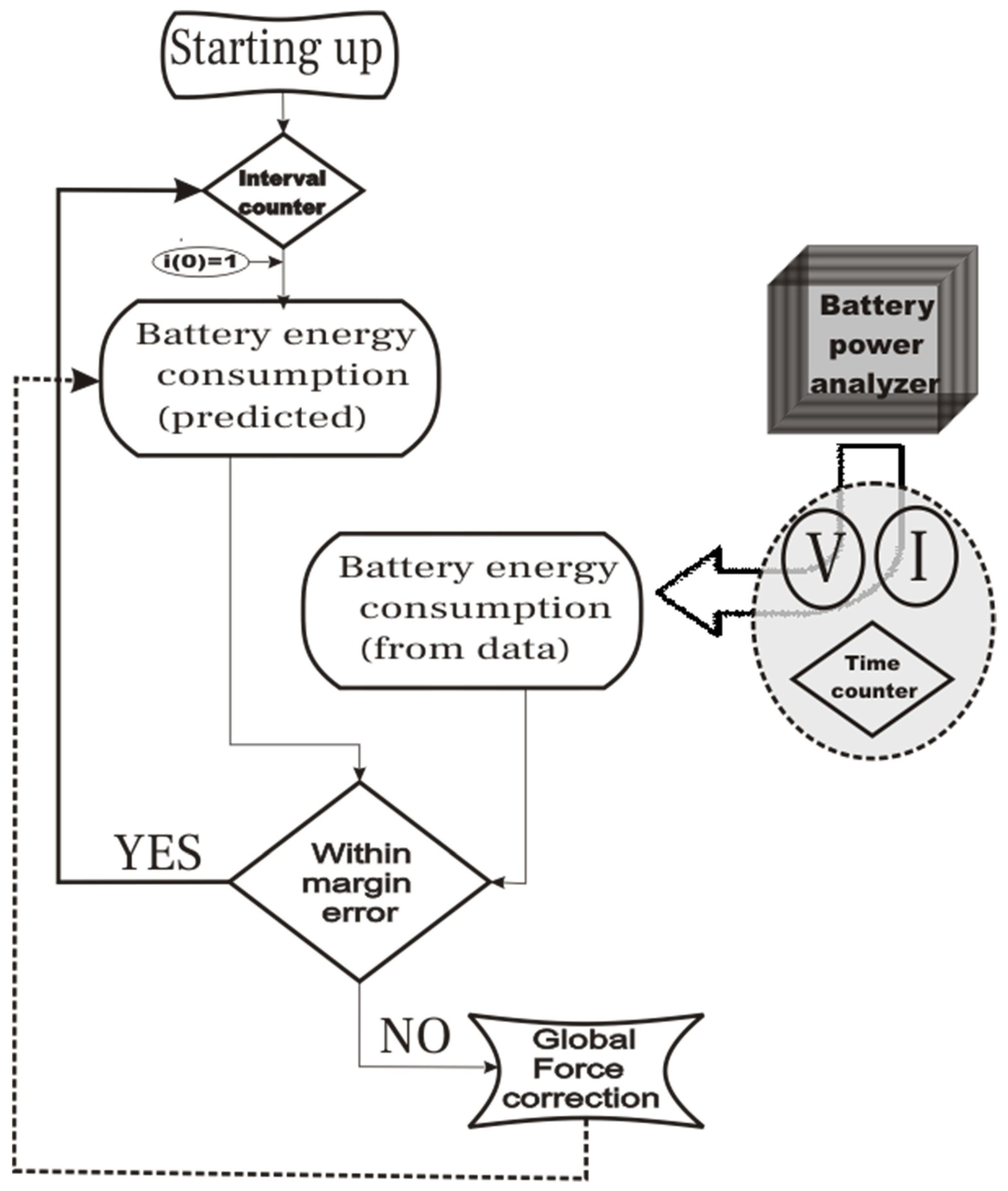
The electric vehicle control unit (EVCU) compares the result from the calculation using Equation (27) with the experimental value from Equation (26). If the two values match within the set-up error margin, the calculated value is considered valid and the program continues to the next time interval. When there is a difference between the two values that exceeds the set-up margin error, the system modifies the calculated global force by a factor that eliminates the difference, and then applies this correction to the remaining intervals of the intercity route, so it recalculates the energy consumption and the driving range. The following diagram shows how the software works (Figure 8).

Corrections in the calculation of energy consumed by the electric vehicle can be attributed to different causes, including variation in the vehicle speed because of traffic, changes in the driving style due to a change in the driver’s attitude during the route, and modifications of the characteristics of the route such as the type of pavement, wind speed, etc. These effects cannot be foreseen before starting the trip, and therefore, cannot be implemented in the predictive calculation method.

4. Experimental Test

To prove the validity of this assessment, we performed an experimental test on an electric vehicle, BMW i3, on a specific intercity route. This route departed from the city of Madrid (Spain) and finished in a small town located 53.3 km north of Madrid City (see Figure 9).

The route is a two-lane highway with no intersections between the starting and destination point. Entering and exiting the highway was considered in the calculation of driving range. A moderate driving style was used with medium acceleration values when required (currently 1.75 m/s²). The characteristics of the route are accessible from any of the current applications used in navigation mode; in our case, Google Maps was selected. The type of pavement was considered regular and homogeneous over the entire route. The data was obtained from public information provided by the Spanish Ministry of Transport, Mobility and Urban Agenda [34] and the Spanish General Directorate of Traffic (DGT) [35]. The aerodynamic coefficient for the BMWi3 model was obtained from the official data sheet provided by the manufacturer [36]. The mass of the vehicle was also taken from the official data sheet [37].

Table 3. Values of the relevant parameters for the simulation process.

Mass of Vehicle (kg)	Aerodynamic Coefficient	Rolling Coefficient	Maximum Slope (°)	Battery Capacity (Ah)	Energy Content (kWh)	Battery Voltage (V)
1600	0.29	0.15	± 5	120	42.2	352

shows the values of the parameters used in the calculation.

The test was performed in both directions along the route to compare results from both cases and verify the quality of the test. The results on the return journey were in good agreement with those of the outward trip, within 99.4% accuracy. Therefore, the test was considered valid for the energy calculation. The results from the two tests, the outward and return trips, were averaged for unity purposes.

Figure 10 shows the results of the test performed for the intercity route case. The continuous line corresponds to the measured values obtained through direct calculation using the registered parameters (voltage, current and time of the battery) and applying Equation (26). The dashed and dotted line represents the values obtained using the predictive method, and dotted line corresponds to the application of the hybrid method.

The test was divided into three different sections. Region A corresponds to the first part of the journey between the Starting Point (SP) and Intermediate Point 1 (IP₁). Region B is between Intermediate Point 1 (IP₁) and Intermediate Point 2 (IP2), and region C is from Intermediate Point 2 (IP₂) to the end of the journey at the Ending Point (EP). The operational method for determining the energy consumption along the route is described below.

4.1. Predictive Method

• Region A

The software calculates the energy applying the predictive mode at intervals of 1 km. At the end of the first interval the electric vehicle control unit (EVCU) evaluates the result from the predictive method and compares it to the data obtained through experimental measurements using Equation (26). In the case of a deviation between the predicted value and experimental data higher than the set-up value, the software applies the correction factor until the deviation falls within the limits and recalculates the energy consumption for the predictive method for the rest of the section range. The process is repeated at every interval of 1 km.

• Region B

The procedure is very similar to the one explained for region A with the only difference that repeating the process is omitted; thus, the calculation of the energy consumption applying the predictive method is based on the calculation at the first interval of 1 km. The method evaluates the deviation between the predicted and measured values and corrects the calculation of the energy consumption through the predictive method over the entire range corresponding to this section B until Intermediate Point 2, with no further corrections applied, no matter if there are deviations or not.

• Region C

No action is taken on the predictive result of energy consumption in the whole range of the region.

4.2. Hybrid Method

• All regions (A, B and C)

As in the predictive method for region A, the software calculates the energy applying the predictive mode at intervals of 1 km for the entire route. At the end of every interval, the EVCU evaluates the deviation between the experimental data and predicted values and applies the correction factor if the deviation exceeds the set-up value. This procedure applies to the whole route.

4.3. Analysis of Results

Looking at Figure 10, it can be seen that the predicted values match reasonably well with the measured results in region A, where correction is applied at the end of every single interval, proving that the application of the hybrid method is of high merit. In fact, the experimental measurements, predictive method and hybrid method show almost identical values of energy consumption for the entire range of the region.

In region B, where predicted energy consumption is based on an initial application of the correction factor at the end of the first interval with no further corrections for the entire range of the region, the predicted results show a slight deviation from the measured results, a deviation that increases with travelled distance. However, the hybrid method closely matches the measured results with very small deviation over the entire range of the section.

In region C, where the predicted values are not corrected at any time, it can be observed that there is a large deviation between the predicted results and experimental data, a deviation that is extended over the entire range of the section. It can also be observed that the deviation is higher when the power demand increases. On the contrary, the hybrid method shows a very good performance with results in close agreement with the experimental data, proving the accuracy of this methodology.

Analyzing the application of the hybrid method over the whole range of the tested intercity route, we observed a close agreement between measured data and hybrid results, with an accuracy higher than 99%. This proves the merit of the hybrid method and the validity of its application at the intercity route case.

5. Conclusions

A new method to evaluate the energy consumption in electric vehicles travelling on intercity routes is proposed. This method consists of a hybrid form of a predictive method and the application of online information during the driving run.

This new method is based on the calculation of the energy consumption using equations from dynamics that provide a prediction for the energy consumption, and thus, for the driving range. The method also uses a correction factor that is applied to the prediction of the energy consumption based on the deviation between prediction results and online data.

The hybrid method uses online information and measured data obtained from the electric vehicle control unit (EVCU), which registers values of vehicle speed, acceleration, slope of the route, battery voltage, and current drained from the battery. The method uses a data base with set-up values of characteristic driving parameters, including rolling and draft coefficients, and the mass and aerodynamic coefficient of the vehicle.

The proposed hybrid method allows the driver to select the style of driving by inputting an acceleration value. Three cases have been considered for driving style: aggressive, moderate, and conservative. These three cases correspond to current options in modern electric vehicles: sport mode (aggressive), cruising (moderate) and ECO (conservative).

This hybrid methodology is of high accuracy if applied at short time or distance interval control. The accuracy in the test case was higher than 99% for a controlled test using a distance interval of 1 km or time interval of 45 s. The accuracy can be improved if the time or distance interval is reduced.

Applying the hybrid method, the calculated energy rate for the intercity route was determined to be 132.0 Wh/km, which is very close to the measured value of 133.1 Wh/km provided by the EVCU. These values are within the current range of the tested vehicle.