1. Introduction
Automated driving is currently one of the most outstanding and ambitious technological developments in the automotive field, to a large extent motivated by the improvement of transport efficiency and driving safety [
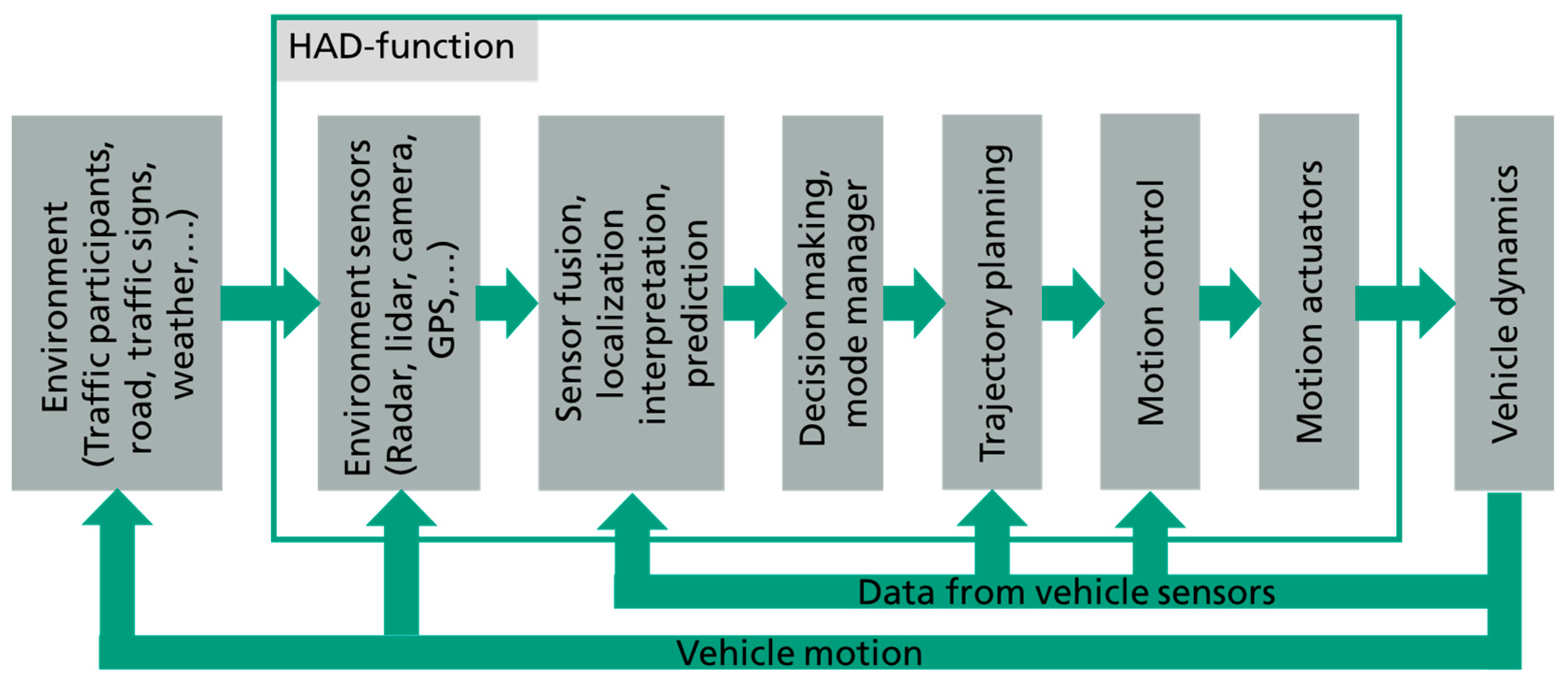
1]. This is supposed to be obtained by replacing the human driver with a complex system including sensors for detecting the environment, a so-called highly automated driving (HAD) function, and actuators. The functionality of such systems is dependent on a high number of technical subsystems. The influence of the functional reduction or failure of components in those systems on the safety of the HAD function can be difficult to predict and depends on the functional relations within the vehicle subsystems as well as on the driving situation.
One of the major challenges of the testing and validation of automated vehicles is covering the enormous amount of possible driving situations resulting from the complexity and high number of variables of the interaction of a vehicle with the environment and other traffic agents. Moreover, automated vehicles need to be tested and validated not only in standard and usual driving situations, but also under severe and extreme conditions. Replacing a large proportion of real driving tests with simulation leads therefore to a major benefit for the development of automated vehicles [
2]. Similarly to other complex mechatronic systems, shifting tests to simulation means also shortening the development process and improving its flexibility. The SET Level project, supported by the German Federal Ministry of Economic Affairs and Climate Action, aims at providing an environment for simulation-based testing and development of automated driving functions [
3]. The project focuses on scenario-based analysis and testing, especially within urban areas.
With the possibility to virtually simulate a vehicle’s behavior, including the functional effect chains of the HAD function in various driving situations, it becomes favorable to also investigate the behavior in cases of component failure systematically during the virtual assessment of the vehicle using fault injection, as suggested by ISO 26262. The application of quantitative measures for emergent risk makes the safety gain in critical situations quantifiable and thus can improve confidence in HAD functions, accelerating the development and approval of automated vehicles for public roads, and thus will foster the breakthrough of HAD, bringing its improvement of transport efficiency and driving safety into effect.
Other works have covered fault injection in HAD function and sensor models [
4,
5]. Specifically, sensor faults are discussed in many other research works, e.g., in the vehicle front sensor and speed sensors [
6], in the GPS and in the steering ECU [
7]. The work of [
8] covers multi-sensor fault detection, identification, isolation and health forecasting. No work from the literature is known, however, that covers a specific actuator component fault in autonomous driving and its influence on the vehicle’s behavior.
In [
9,
10], a simulation framework for virtual testing of autonomous driving functions including effects of vehicle dynamics in a closed-loop manner was presented. In this paper, this framework is extended for use in virtual testing of autonomous driving functions under the influence of a fault occurring in a component. Furthermore, functions for calculating standard criticality metrics for driving scenarios are added. Models for the simulation are presented in
Section 2, consisting of trajectory planning, motion control and a vehicle model. Fault-handling tests in a right-turn maneuver subject to an injected fault in the steering system are described in
Section 3. Different scenarios are discussed without and with a fault and without and with counteractions against the fault. The results of five scenarios for different criticality metrics are discussed in
Section 4.
2. Models and Simulation Framework
This section introduces the simulation framework for the testing of autonomous driving functions. Furthermore, the models used in the tests are described in detail.
2.1. Simulation Framework
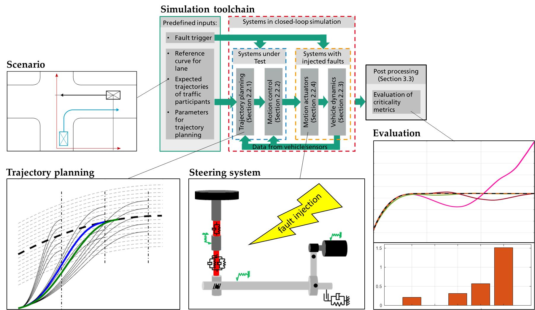
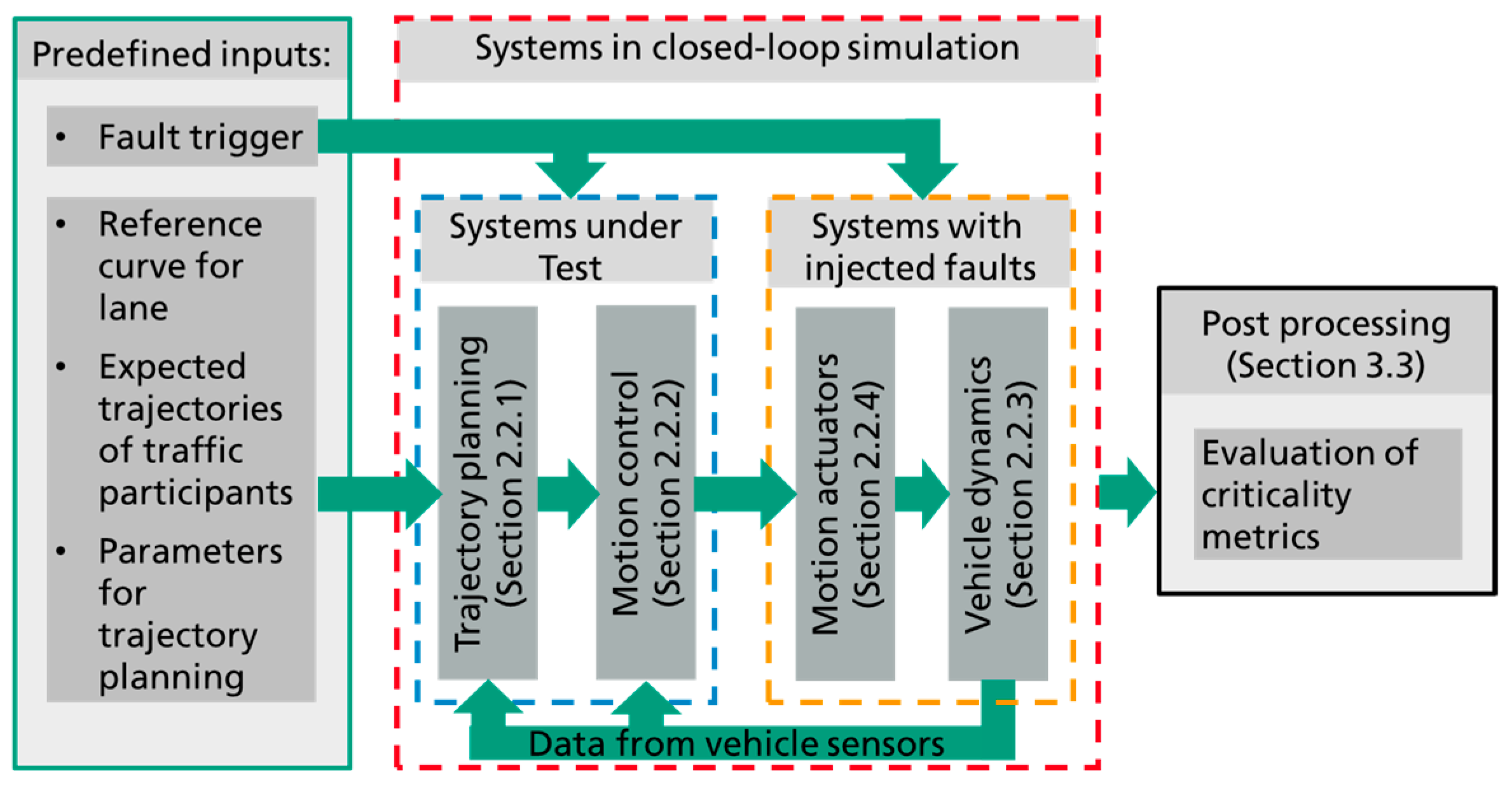
For each simulation task, an appropriate simulation set-up needs to be selected. Whereas the functionality of some subsystems and components may be analyzed in open-loop simulations with pre-defined input signals, the analysis of the behavior of interactive systems requires closed-loop simulations. The selection of the subsystems to be included into a simulation depends on the purpose of the test.
Figure 1 shows the flowchart of a numerical simulation of an autonomous vehicle driving in a traffic scenario.
In a closed-loop simulation of a traffic scenario, traffic participants may react to the behavior of the ego vehicle under testing. Such simulations are useful for analyses with a focus on the behavior of the ego vehicle and its external communication. For analyses focusing on scenario perception of the sensors, traffic participants do not need to act in a closed-loop, but the impact of vehicle motion on sensor view is of great importance.
For designing and testing a vehicle’s motion control, the feedback loop of the control system consisting of motion controller and the controlled vehicle dynamics and actuators need to be included in a closed-loop simulation. Trajectory planning may need to be part of this control system, too, because it may react to position deviations with an updated trajectory, whereas the input from other subsystems can be provided statically as open-loop input. All these different simulation set-ups with their different focuses can be implemented using the simulation framework developed in SET Level.
Numerical fault injection tests may serve either for verification of system requirements or for identifying critical degraded conditions and the development of feasible vehicle-degraded modes for the HAD function. Such tests are of course relevant for all subsystems of an autonomous vehicle, including sensors, software, actuators and the mechanical vehicle systems. The required levels of detail for the subsystems included in the simulation differ depending on the failure modes under investigation and the system under test (SUT). Whereas fault injection tests with faults in the sensor and parts of the HAD software, which are upfront of the trajectory planning, require only very simple vehicle models like a kinematic single-track model, testing of trajectory planning and motion control requires a higher level of detail for the vehicle model. The simulation set-up described in this paper is designed for fault injection tests, which require a high level of detail in the vehicle dynamics model; this includes, e.g., failure modes, which affect the dynamic response of the vehicle to inputs from the controller. Such failure modes may affect the lateral and longitudinal controllability of the vehicle and hence may result in hazardous situations. In this case, the SUT is the trajectory planning and motion control of the vehicle. Trajectory planning must be able to plan trajectories which are feasible for the vehicle in its degraded state, and the motion control system must be able to make the degraded vehicle follow this trajectory with acceptable accuracy, at least for driving the vehicle into a minimal risk condition. Out of the subsystems depicted in
Figure 1, the trajectory planning, motion control, actuators and vehicle dynamics models are included in a closed-loop simulation for this kind of test, whereas the expected trajectories of traffic agents as well as the reference curve to follow are used as open-loop inputs from “decision making”, “prediction” and “mode manager” (see
Figure 2).
This selected simulation subsystem is feasible for tests with the purpose of verifying robustness of the motion control and the feasibility of trajectories for the degraded vehicle state, as well as for designing and testing failure-degraded modes of the HAD function, which may include modified parameters for trajectory planning, motion control and actuator management. Furthermore, failure modes can be identified for which the vehicle journey needs to be discontinued, and corresponding minimal-risk maneuvers for transferring it into a minimal-risk condition can be identified.
The simulation as well as the postprocessing are set up in a MATLAB/Simulink environment. In this environment, the simulation is controlled by a MATLAB script defining all the “predefined inputs” listed in
Figure 2 as a function of time and starting the simulation run of the Simulink model, which contains the subsystems included in
Figure 2 in the “systems in closed-loop simulation” box. Each of the subsystems has a standardized in- and output interface to enable exchangeability of each submodel without any need to adapt other submodels. After completing the simulation run, the resulting vehicle motion is handed over to a MATLAB function, where the assessment of the simulation results is performed in an offline post-processing environment using a variety of criticality metrics (see
Section 3.3). The models included in the simulation set-up are described in the following sections. The reference to the corresponding section is denoted in
Figure 2.
2.2. Individual Models
In this section, the model components of the toolchain (first introduced in [
9,
10]) are described. Starting with trajectory planning and motion control, the section also describes the vehicle dynamics and actuator models used in this work.
2.2.1. Trajectory Planning
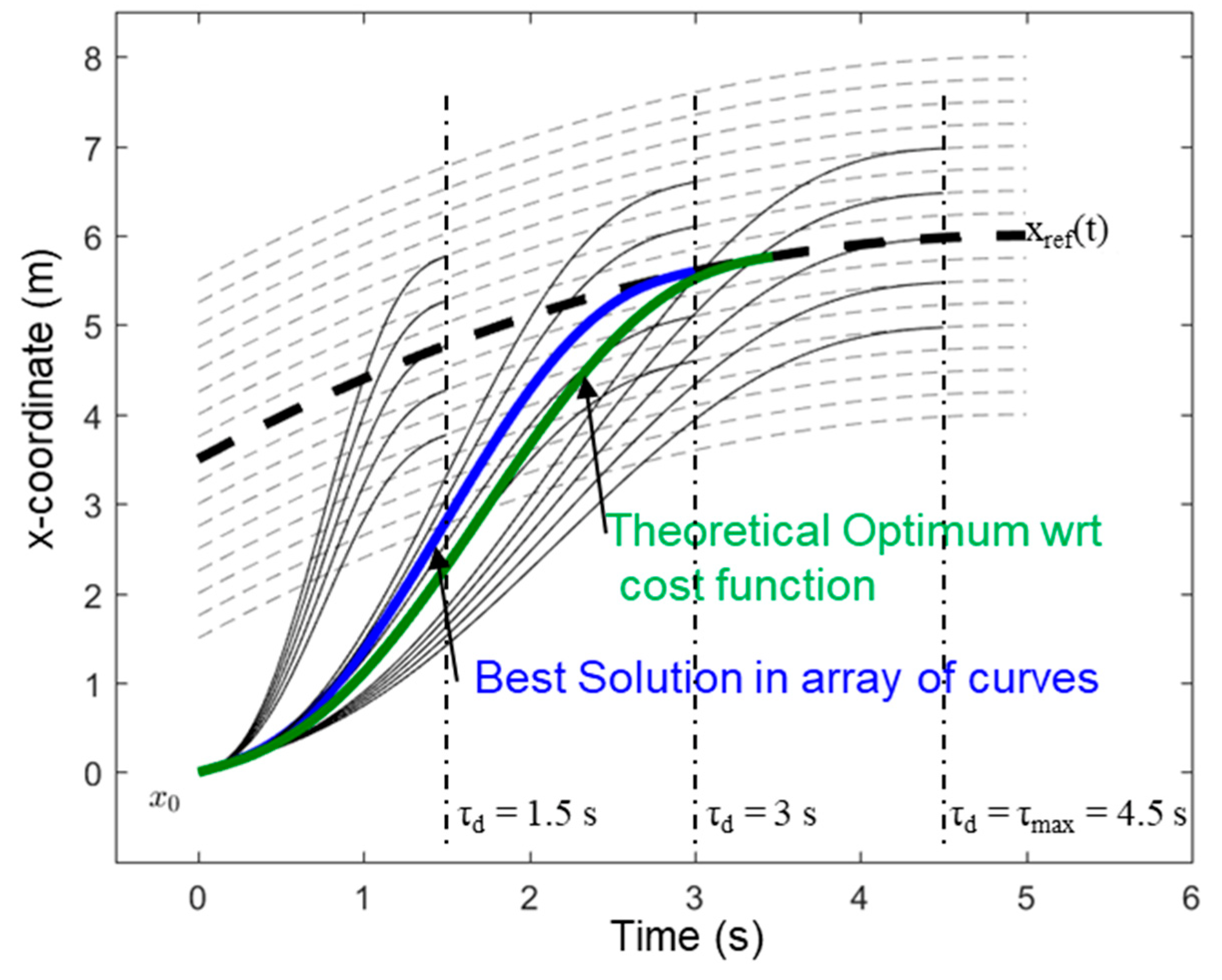
The trajectory-planning algorithm used in the model chain for the investigations uses discretized terminal manifolds, as proposed by Werling et al. [
11]. Within this algorithm, a manifold of trajectories is created, amongst which the best with respect to given boundary conditions and quality criteria is selected. The algorithm creates the manifold of trajectories by varying polynomial functions, which are expressed in Frenet coordinates relative to a predefined reference curve, e.g., the centerline of the lane to follow. The polynomial functions for longitudinal (Equation (1)) and lateral (Equation (2)) movement are created independently.
In these equations, s denotes the longitudinal position of the vehicle projected perpendicular to the reference curve, d denotes the lateral distance, and t denotes the time (start time of each trajectory is t = 0). The coefficients c… of the polynomial functions are chosen so that they minimize the jerk in the trajectory for given initial and end conditions of the trajectory. The initial conditions are identical for all trajectories. Normally, they are taken from the planned state according to the previously selected trajectory after one planning time step. In the case that the difference of the actual vehicle position and the actually planned position exceeds predefined limits, the initial conditions are computed based on the actual vehicle position using an extrapolation to the expected vehicle position at the beginning of the next planning time step. For creating the manifold, the end conditions are varied. The varied parameters are the final longitudinal position , the final longitudinal velocity , the final lateral position as well as the durations and for reaching the final longitudinal and lateral positions, respectively. The end condition for the lateral velocity is always , which means that all trajectories end with a vehicle movement parallel to the reference curve. Furthermore, the acceleration at the end of all created trajectories is zero. If the duration parameters and are smaller than the planning horizon , the trajectories contain a constant longitudinal velocity for and a movement with constant distance to the reference curve for . First, the algorithm creates manifolds of lateral and longitudinal trajectories independently. Then, the full manifold of trajectories is created by combining each lateral trajectory with each longitudinal trajectory.
For all the trajectories in the manifold, the trajectory-planning algorithm checks whether they satisfy the given boundary conditions, such as the limitation of total horizontal acceleration due to tire friction, limit of curvature, limits of engine torque and engine power, maximum velocity and accessible lane width. Furthermore, in the presence of other traffic participants, a collision check algorithm ensures that safe distances in space and time are respected. Out of all the trajectories which comply to these boundary conditions, the one is selected which has the minimal costs according to the cost function
It considers the lateral jerk
and the longitudinal jerk
, the difference of the final velocity
and final lateral position
from their reference values (
for velocity and
for lateral position) as well as the durations
and
until the final state is reached.
Figure 3 shows an example of a manifold of lateral trajectories.
In the end, the selected trajectory approximates the theoretical optimum with respect to the cost function. The quality of the approximation depends on the discretization of the manifold.
2.2.2. Motion Control
The task of the motion controller is to control the lateral and longitudinal motion of the vehicle according to the trajectory planned by the trajectory planner (see
Section 2.2.1). It considers the deviations of the actual vehicle state from the planned vehicle state in longitudinal position
, longitudinal velocity
, lateral position
and heading angle
. All these quantities are computed in the actual vehicle body coordinate system. Based on these deviations, controller commands for lateral acceleration
and curvature
are computed. These controller commands are inputs to the actuator management system (see
Section 2.2.4). By choosing kinematic quantities at the interface between motion control and actuator management, the interface becomes independent from the actual vehicle design, which is a benefit with respect to the exchangeability of submodels. The control laws are given below.
The longitudinal motion is controlled using the linear approach given in Equation (4). The acceleration command uses the planned acceleration from the trajectory and adds an amount of acceleration depending on the controller deviations and and the controller gains and . Steering control (Equation (5)) works similarly, using the planned curvature , adding curvature based on the deviations and and the controller gains and , but it contains some nonlinear features: The amplification of the curvature command depends not only on the controller deviations, but also on vehicle speed as denoted in Equation (5). The higher the vehicle velocity is, the smaller are the steering commands. This part of the control law is intended to make the lateral velocity in steering maneuvers independent from the vehicle speed, making the controller feasible for a large velocity range. Equation (6) expresses a degressive behavior of the curvature command with increasing values of the desired curvature correction . This nonlinearity considers the nonlinear steering behavior which is caused by the limitations of the steering actuation. The steering actuation can follow small-amplitude commands with higher frequency than large-amplitude commands. Hence, also the stability of the control loop depends on the command amplitude. This is compensated by this degressive behavior, which reduces controller amplification with an increasing value of , which corresponds to an increasing controller deviation. Furthermore, the steering control includes a static pre-control feature. It accounts for non-kinematic vehicle behavior. Due to tire slip, the vehicle does not perfectly follow the commanded curvature. This difference, which increases with increasing velocity and increasing lateral acceleration, is approximated by the function given in Equation (7). This approximation of the ratio of the actual and the requested curvature is used to compensate for this non-kinematic behavior.
2.2.3. Vehicle Dynamics
The vehicle dynamics model implements a reduced 3D multi-body model of the vehicle chassis with suspensions and the tires. As inputs, the model receives the output signals of the actuator models (i.e., the rotational velocity of the wheels, the reaction powertrain, braking torques and the steering rack position). As outputs, the model delivers the required feedback signals to the actuator models (i.e., wheel torque to the powertrain model and steering rack force to the steering model) as well as several signals describing the vehicle dynamics (such as translational and rotational velocities, accelerations, etc.).
The chassis part of the vehicle dynamics model includes rigid bodies for the car body (or sprung mass) and four unsprung masses, connected to the sprung mass by the suspension constraints and by the suspension stiffness and damping elements. The dynamics of the sprung mass are described by its 6 degrees of freedom (DOFs). This body is connected via the suspension constraints to the two front unsprung masses, each of them with two relative 3D-spatial DOFs, representing the suspension travel and the steering rack movement. Similarly, the sprung mass is connected to the two rear unsprung masses, each of them with just one relative 3D-spatial DOF, representing the suspension travel (i.e., no rear steering is implemented in the model). Finally, each unsprung mass is connected to the respective wheel by a relative rotational DOF about the wheel rotation axis. Because the wheel rotations and the steering rack position DOFs are imposed as so-called motions from the input signals, they do not account for the total number of DOFs of the system, which are then 10 in total.
The suspension constraint is modeled as a pure kinematic 3D constraint involving all six coordinates as function of the displacement along the vertical coordinate
of the unsprung mass center relative to the car body and of the steering rack displacement
(the latter, as mentioned, just for the front axle). The suspension constraint can be simply written as
where
represents the vector of all translational and rotational coordinates of a single unsprung mass. The spring displacement and the damper velocity are defined in the same way. All these kinematic functions are modeled as polynomial functions by fitting experimental data or data obtained by models with higher levels of detail (such as complex multi-body models).
The main equations system of the model is built by combining the suspension kinematic Equation (8) with the dynamical equilibrium equations of the sprung and unsprung masses as well as the equations of force equilibrium along the suspension DOFs. The latter are written using the virtual work principle and involve the suspension loads
and the spring, damper and anti-roll bar forces. The resulting equation system is symbolically manipulated; this leads to a linear function with respect to the accelerations of the Lagrangian coordinates
(i.e., the system DOFs) and the Lagrangian multipliers (i.e., the suspension loads
). These can be therefore obtained by solving the following linear problem
where
represents the tire loads,
the aerodynamic load,
all torque inputs (from powertrain and braking system) and
the wheel rotation velocities. The velocities and the Lagrangian coordinates are then simply obtained by integration from the accelerations.
The tire loads
are provided by the tire part of the vehicle dynamics model. The horizontal forces and the three moment components are implemented by means of the Magic Formula tire model by Pacejka [
12]. The vertical tire force is obtained by simulating a simple spring–damper-equivalent system, which represents the tire vertical compliance. This allows the model to simulate the main effects of tire interaction with uneven road profiles, even if this simplified approach is mainly intended for use for handling simulations and not for comfort and durability. The tire slip behavior is modeled with a dynamic system of the first order, whose time constant depends on the so-called tire relaxation length and on the tire longitudinal velocity.
Because the classical tire slip formulation leads to numerical problems at speeds close to zero, the tire slip dynamics are implemented with the modification suggested in [
13], which allows the vehicle to fully stop and restart, as required for simulations for the testing and validation of autonomous vehicles.
2.2.4. Actuators with Management
The actuator management model implements a simplified control, which converts the drive signals from the motion control into the target signals for the powertrain, braking and steering actuators. The drive signal of the longitudinal acceleration is used to compute the target powertrain and brake torques using algebraic functions. For this purpose, a simple point mass model for longitudinal dynamics is implemented in the algorithm, which takes into account some basic powertrain and vehicle parameters (such as the torque–velocity characteristic, the maximum torque and power values and the wheel radius). In terms of steering, the actuator management model uses the pinion angle of the steering model as an input to calculate the current rack position . This is compared to the target rack position, derived from the target curvature by means of ideal Ackermann steering. A PID controller is used to minimize the difference between the actual and target values. An optimization algorithm is used to find suitable controller parameters, considering the maximum overshoot, the time delay and the residual difference at a defined time in a step response test.
The steering system (cf.
Figure 4) consists of the steering actuator and the steering kinematics model, which comprises all mechanical parts transferring torque from the steering wheel or actuator to the tie rod. The steering system investigated is an electric-powered steering (EPS) system with belt drive that acts on the rack via a ball nut mechanism. The inertia and compliances of the mechanical parts are split into a 3DOF model as proposed in [
14].
The steering wheel and column are considered as two inertias. The third inertia is steering pinion, ball nut assembly, rack and steering actuator, which are kinematically coupled via the pinion–rack–gear ratio. Advanced friction elements acting on the steering column, steering rack and electric motor comprise exponential spring friction elements and a Maxwell element; see [
15]. The steering actuator contains a model of the electric motor and a torque controller. It converts the desired pinion torque from the actuator management system to an actuator torque that acts via the belt drive on the steering rack.
The powertrain model consists of an electric engine model and a transmission model. The latter includes a differential for the driven axle and wheel models for the driven and non-driven axle. A target torque
as an input from the actuator management system is converted to an actual torque by the motor model. The motor model is represented by a PT1-element with a time delay
together with a lookup table limiting the motor torque to a maximum torque
. The motor torque
is transferred to the differential gear and is split up into equal torques
and
for the left and right wheels, respectively, as
where
is the transmission ratio and
the transmission efficiency. For a single wheel, the equation of motion can be written as
with the wheel reaction torque
, the braking torque of the respective wheel
, the rotational wheel velocity
, the rotational viscous damping
and the wheel and motor inertias
and
, respectively. The wheel equations for the non-driving axle are simplified to
The braking system model converts the wheel angular velocities and the target braking torques from the actuator management system into the actual braking torques . The brake actuator is modeled as a PT1 element with time delay representing a hydraulic actuator. A condition for stick and slip friction is implemented using a threshold angular velocity.
3. Fault-Handling Tests
In this section, the usage of the model chain for fault-handling tests and result assessment using criticality metrics is demonstrated using the example of a steering failure.
3.1. Failure Modes
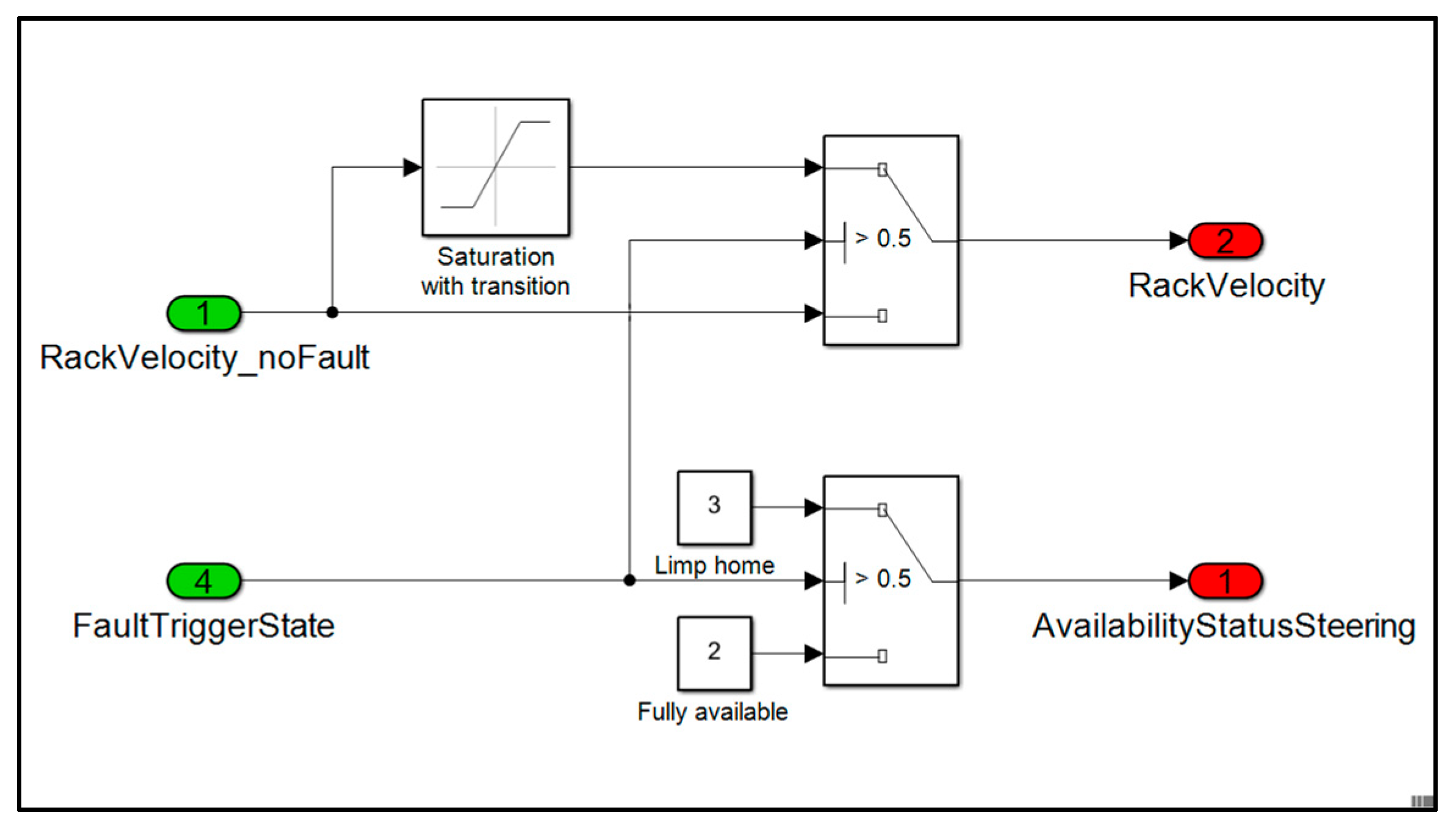
The simulated fault case describes an error that manifests itself in a sudden limitation of the steering actuator velocity (cf. “motion actuators” block in
Figure 2), which directly relates to a limitation of the rack velocity and of the pinion angular velocity
. This error represents a family of errors, which lead along a causal chain to the same degradation of the steering system. One possible fault chain for this fault to occur could be that within a redundantly designed steering actuator, the controller of one branch could detect a severe error, due to, e.g., a missing sensor feedback, which again has its origin in the failure of a sensor or a cable brake. This one branch of the steering actuator will then shut off so that the overall steering actuator operates similar to having only half of the regular motor. In driving conditions with dynamic steering actuation, this results in a severe reduction of possible maximum steering actuator velocity. Only this reduction of the steering angular velocity is modeled explicitly and not its possible origins.
In this work, the fault case is simulated both without and with a detection and counteraction to show the difference with respect to criticality metrics. As the focus of this work is to investigate interactions between degraded vehicle system dynamics and a highly automated driving function, the implementation of fault injection does not consider the full fault chain, as described above. The fault is considered in the MATLAB/Simulink model of the mechanical part of the steering system using logical inputs and operators to trigger a saturation block, which limits the rack velocity to a constant value. The rack velocity limit is chosen by the authors to cause an angular velocity limit of the steering column of
270°/s. In
Figure 5, strongly simplified elements are used to sketch how the fault trigger affects the output of the steering system. On the one hand, the actual rack velocity is limited in case of a fault, and on the other hand, the steering systems availability status switches from the value 2 (indicating the system is fully available) to the value 3, indicating the degraded state of the steering system. At any time, this state of availability status of steering can then be used as an input to the components of the trajectory-planning and motion control system. Considering the taxonomy mentioned in [
16], the fault magnitude can be described with
, the fault activation time is directly at the start of the simulation, and the fault exposure duration is until the end of the simulation.
3.2. Scenarios
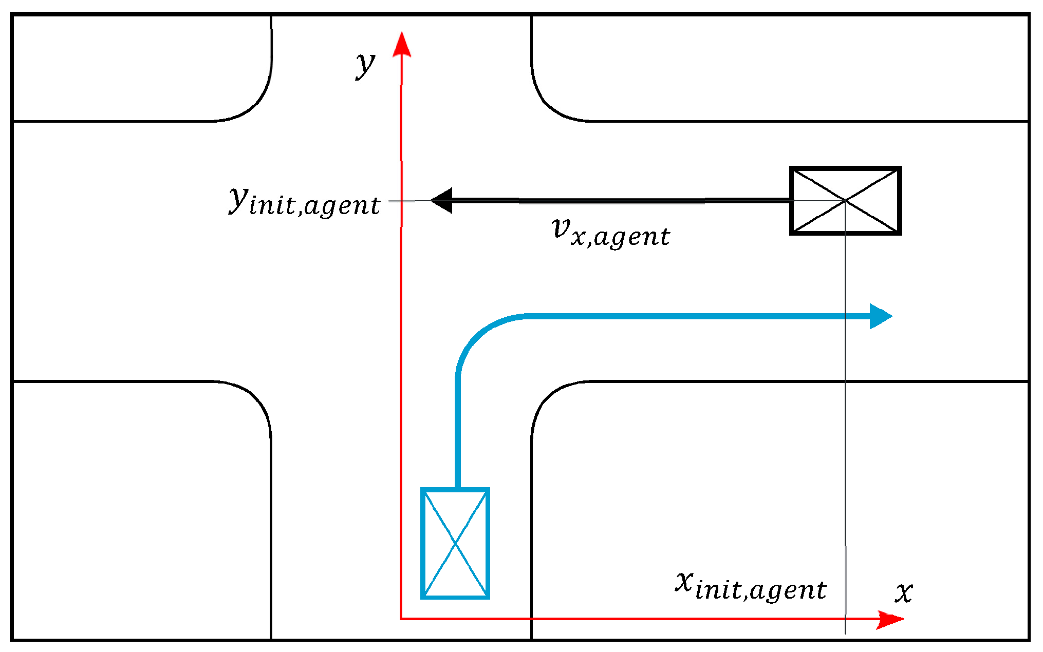
The simulated traffic scenario is a right-turn maneuver of the ego vehicle shown in
Figure 6. The figure shows a crossing with the ego vehicle and a traffic vehicle emerging from the street, the ego vehicle is driving into the street. In the figure, arrows indicate the intended directions of travel.
The conducted simulations of the ego vehicle are shown in
Table 1. The main fault-related parameters for the simulations are whether a fault is injected or not, whether the fault is detected or not and two measures to counteract the fault effects. The measures are an anti-windup in the steering controller and a reduction of the vehicle speed. The term windup stands for a control loop misbehavior triggered by a control value limitation and hence a deviation from linear behavior. Anti-windup describes a counteraction to this problem, which is described in [
17].
3.3. Criticality Metrics
For the calculation of the investigated criticality metrics in this work, the center points of the ego vehicle and the traffic agent are used. On the one hand, the deviation of the vehicle from the planned trajectory is taken as a metric. This metric becomes critical, when a certain threshold value is exceeded and not critical if it remains below this threshold. On the other hand, typical criticality metrics [
2] are calculated using the simulation toolchain. These are represented by the well-known time-to-collision (TTC) metric, calculating the time it would take for two traffic agents (ego vehicle and agent vehicle) to collide in the case of linearly extrapolated trajectories [
18]. For the investigated two-dimensional scenario, a time is calculated when the two traffic agents (1 and 2) approach the same
-position (Equation (13)) and another for the same
-position (Equation (14)).
When both values are the same, a collision happens, and the respective value is taken as the TTC.
is the velocity of the agents that is split up into
and
components for the calculation. The TTC extrapolates the current positions, headings and velocities of both vehicles and determines if a collision can happen between these two trajectories. Other definitions of the TTC are used in the literature [
19], but especially when the vehicles are very close, this definition is reasonable. If no collision happens, the TTC equals infinity. In this case, it can be regarded as noncritical. The TTC is regarded as critical if it becomes lower than a defined threshold value.
Furthermore, the post-encroachment time (PET) [
20] is calculated, which determines the time difference of the two vehicles passing the crossing of their trajectories with the crossing time
of the two agents in Equation (15).
The PET only provides a defined value if a crossing of the two regarded trajectories occurs. Similarly to the TTC, it is regarded critical if it becomes lower than a certain threshold value, which naturally requires it to have a defined value. If it is not defined, it is regarded not critical.
4. Results
The simulations are conducted according to
Table 1. In the first part of this section, the results for the movement behavior of the ego vehicle are presented. In the second part, the criticality metrics for a parameter variation of the starting conditions of the obstacle vehicle are shown.
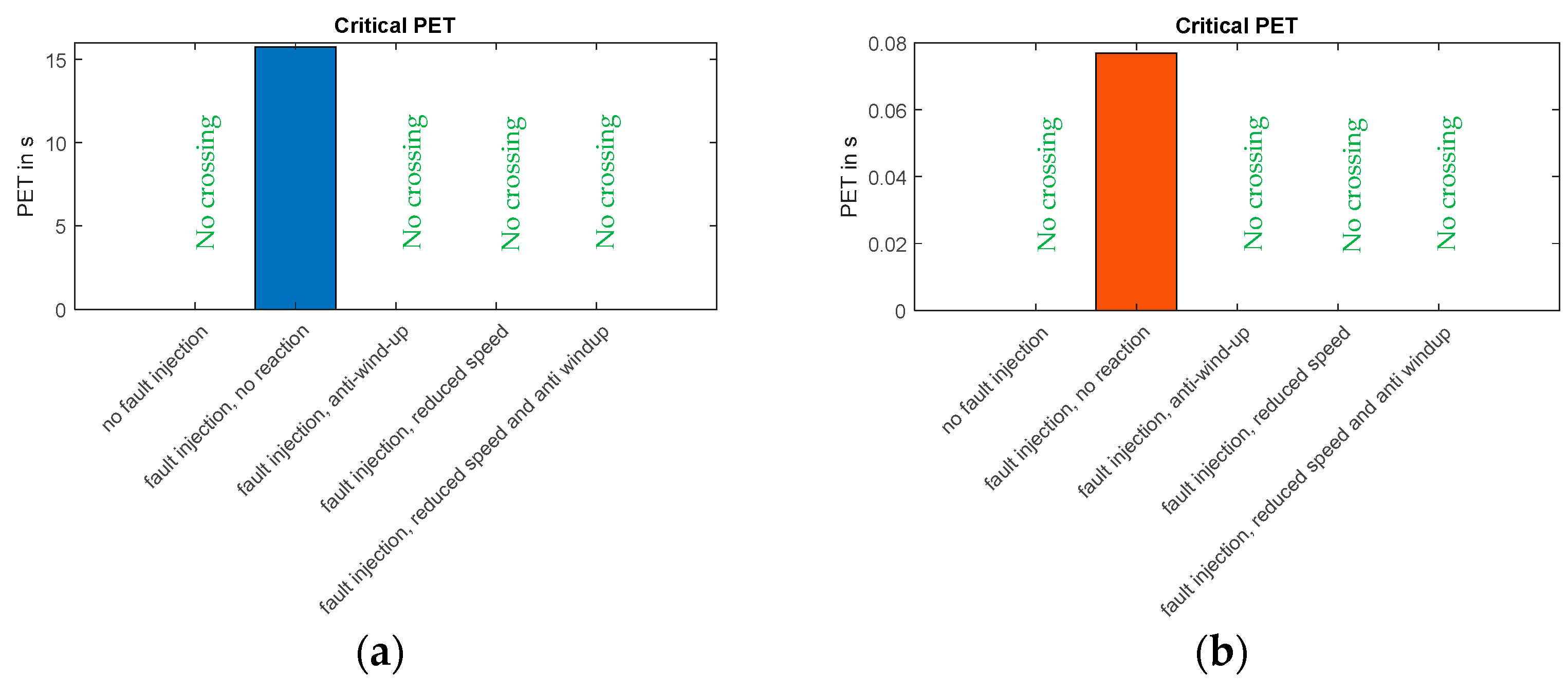
4.1. Simulation Results of the Ego Vehicle
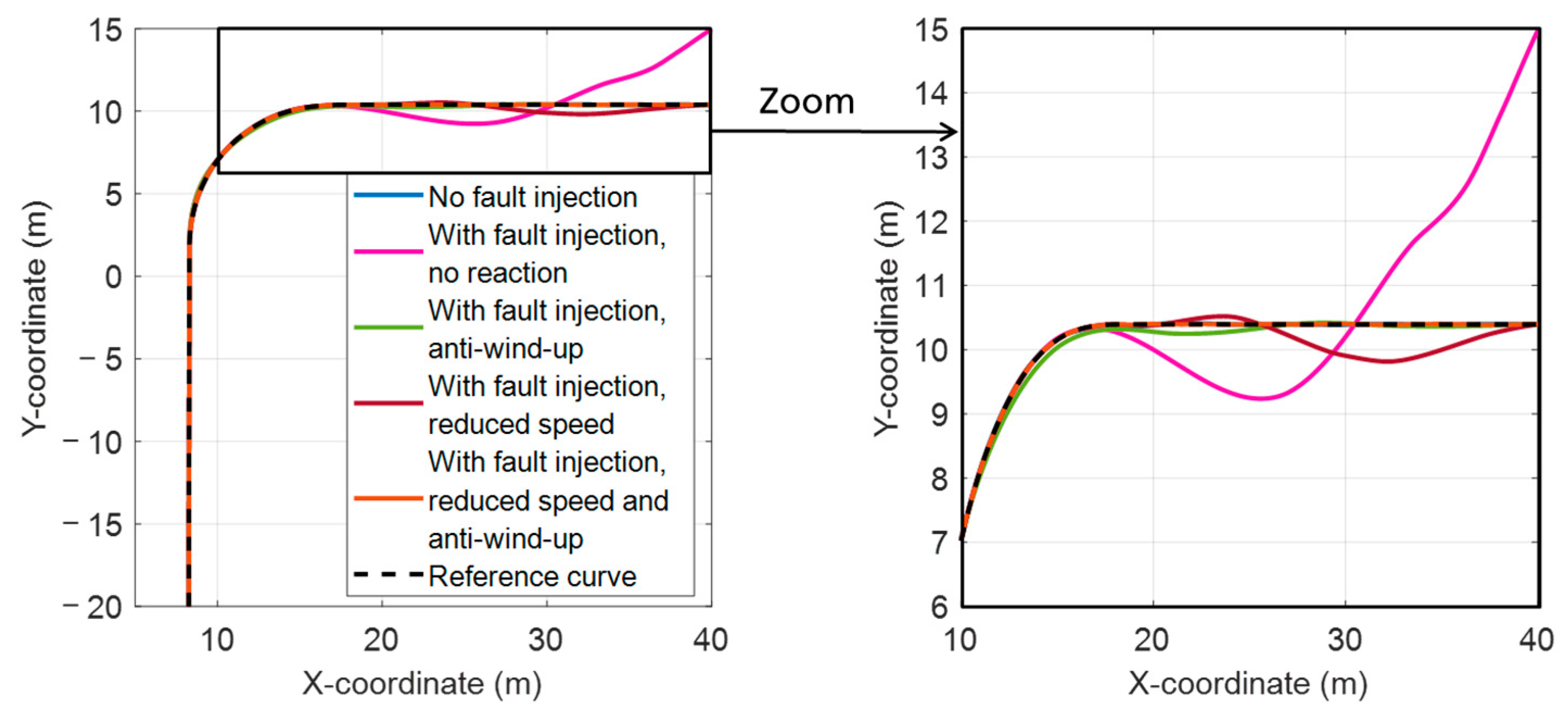
In
Figure 7 the path of the ego vehicle is shown for the different simulation cases. In
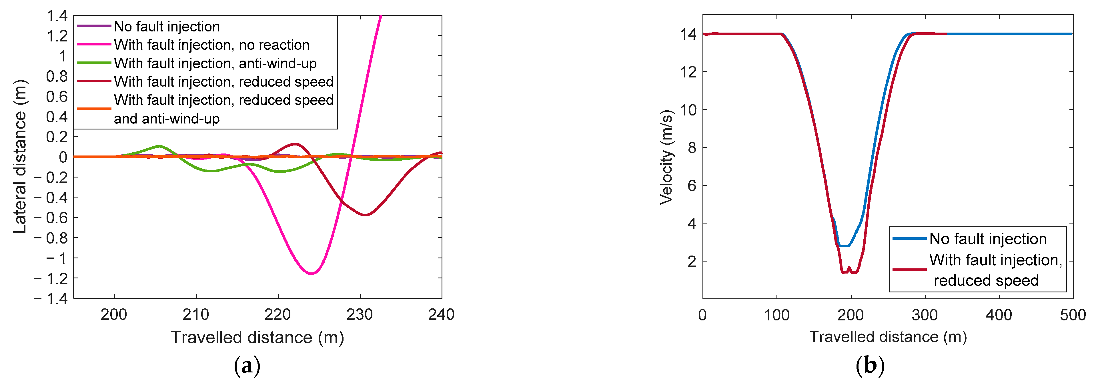
Figure 8 (left-hand side), the lateral position deviation is shown. Without fault injection, the vehicle can follow the reference curve with a lateral distance below 0.031 m. The discussed fault in the steering system leads to a pronounced deviation from the reference curve, which can be explained as a consequence of a windup effect in the steering controller. Without a fault detection, the fault can therefore potentially cause safety-critical driving situations. Using an anti-windup measure in the controller and a reduction of the ego vehicle speed separately, the lateral position deviation can be reduced, but is still noticeable. In the last case, when both measures are combined, the position deviation is reduced to values below 0.01 m. The right-hand side of
Figure 8 displays the planned vehicle velocity with and without the speed reduction measure, showing that the trajectory-planning algorithm reduces the minimum speed in the curve from 2.8 m/s to 1.4 m/s in the case of using the “reduced speed” option.
4.2. Scenario Assessment Based on Criticality Metrics
The values of the criticality metrics depend on the behavior of the other traffic agents. To assess the criticality of an injected fault in a given traffic situation, the most critical behavior for these traffic agents has to be identified. This is accomplished in the following way: The traffic vehicles’ initial x and y positions are varied with a constant velocity of 30 km/h. For all the resulting cases, an evaluation of the TTC (Equations (13) and (14)) and the PET (Equation (15)) is conducted in postprocessing. For the parameter variation, the trajectory of the ego vehicle is not changed in the respective case and remains as shown in
Figure 7.
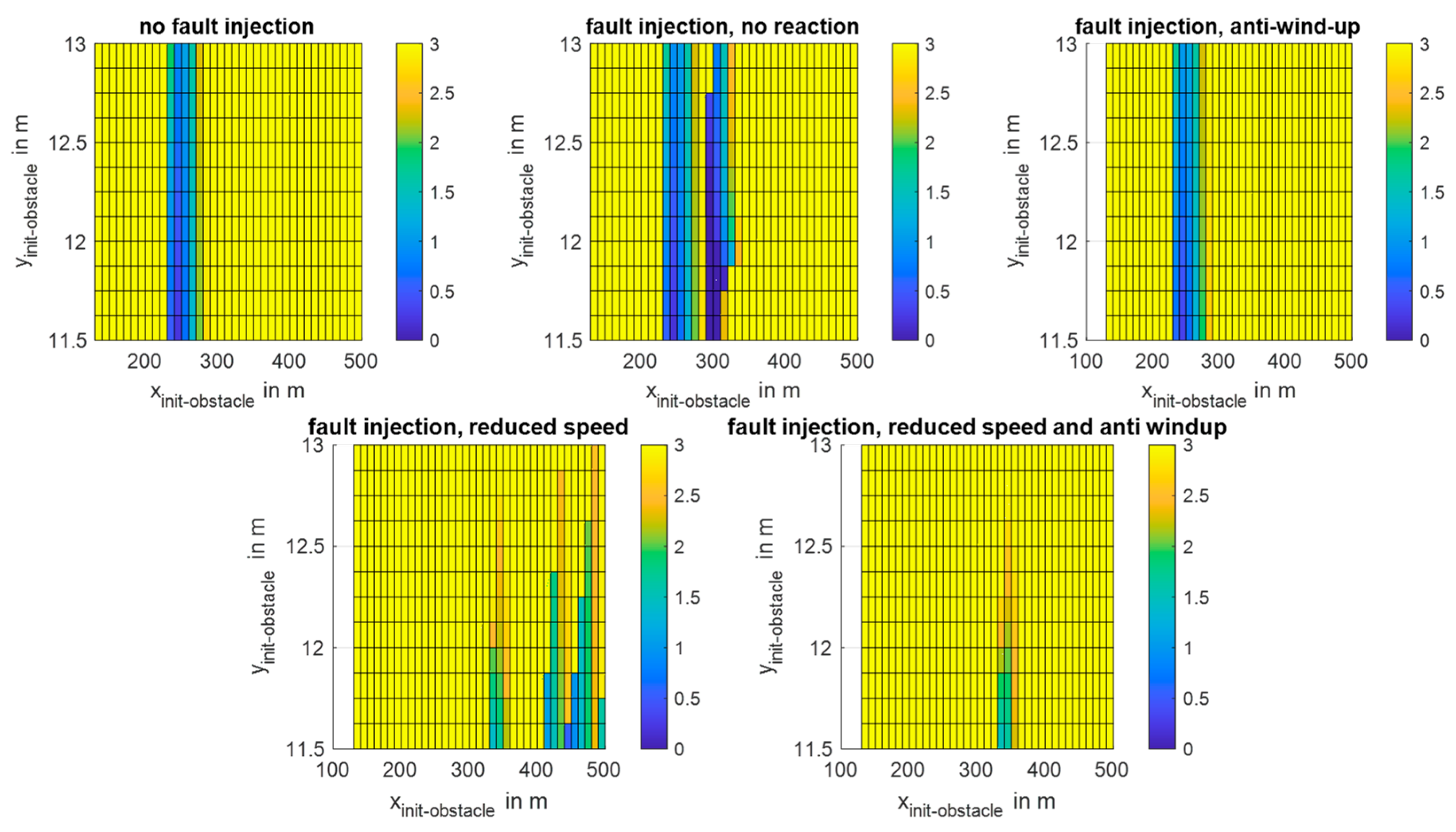
In
Figure 9, the results of the parameter variation in terms of the TTC are shown. To illustrate the effect of the fault, the color map ranges only from 0 to 3 s, as all values above that range are considered safe. First of all, for all cases a TTC below 3 s is observable. However, an additional minimum due to fault injection is observed in the second plot, providing the lowest values of all plots. The safety measure “anti-windup” leads to an improvement in the overall TTC values, achieving a similar behavior as that without a fault. The safety measure “reduced speed” leads to another distribution of the TTC minima, as the vehicles approach each other at different times. The minimum is visibly increased in comparison to the case without a safety measure. Using both safety measures, a strong increase in the overall minimum TTC values is achieved.
In
Figure 10, the mean and minimal values of the minimum TTC values of all simulations in the parameter variation are presented. The mean value condenses the information of the whole parameter study; however, its value strongly depends on the chosen parameter range. The minimum value represents the most critical situation. It can be seen that the mean value decreases in the fault case but increases slightly due to the anti-windup system. The reduced speed, however, decreases the value even more. For the minimum TTC values, the lowest and therefore most critical value is obtained in the case of a fault injection without a reaction with a value close to zero. Both safety measures increase the value. Using the combined safety measures, the mean minimum is slightly increased, and the minimal minimum is increased significantly in comparison to the initial state. This indicates a decrease in the dynamic behavior of the vehicle, which might be safer but not necessarily desirable in practical use. This conflict of objectives is easily understandable when approaching a vehicle velocity of zero. However, for a vehicle suffering from a component fault, a higher TTC threshold value appears to be a reasonable aim of the HAD function.
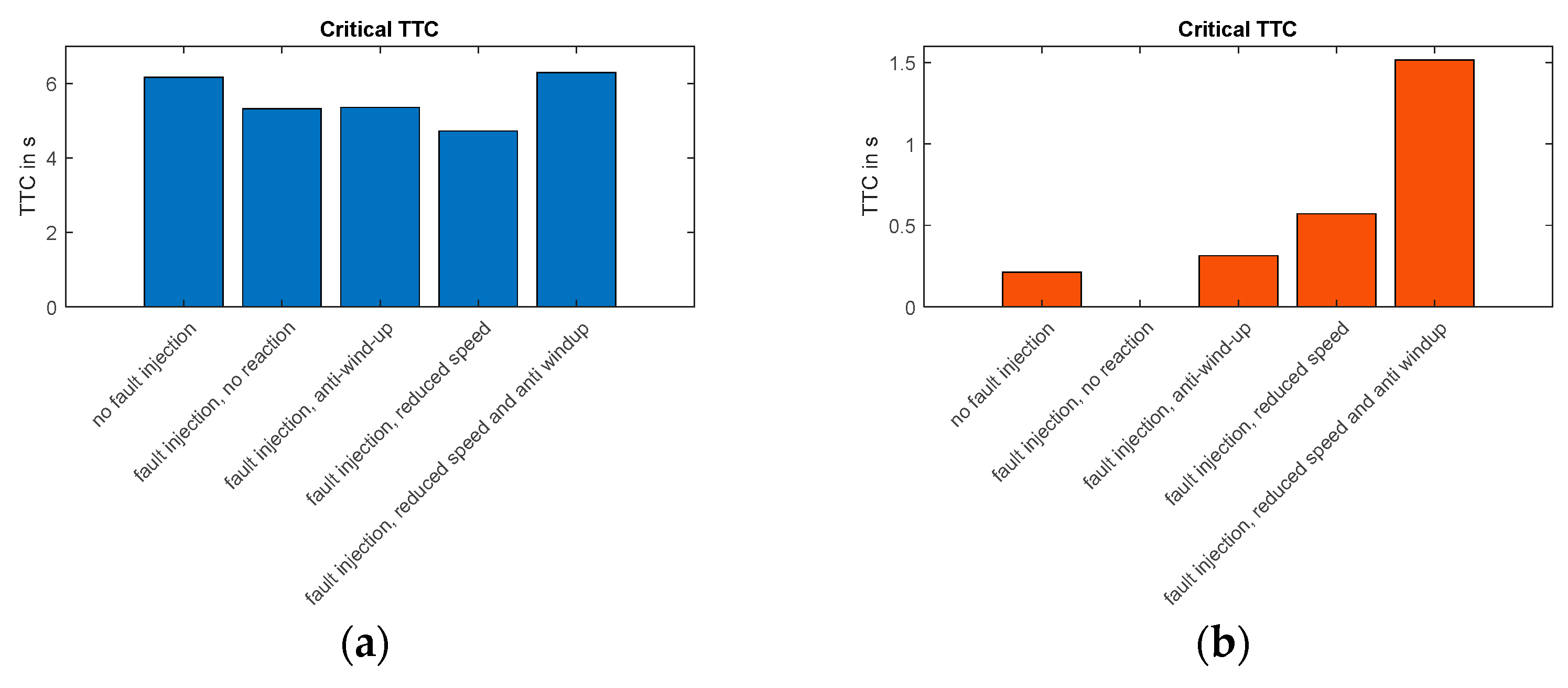
The PET takes the actual driven trajectories and determines the time difference in terms of Equation (15). If no crossing point exists, the PET is not defined. Using the same parameter variation as with the TTC, the results depicted in
Figure 11 are obtained.
It can be seen that only in case of a fault without reaction is a value obtained, as only in this case do the trajectories cross each other. The mean value is relatively high, as only certain parameter combinations result in a short time delay of both vehicles. The minimum value, however, is very low at 0.075 s, representing a very critical situation due to the injected fault. Considering that the vehicles are treated as points for metric calculation, this would certainly lead to a collision of the two vehicles.
The results show that the TTC metric is sensitive to situations where the vehicles approach each other and their linearly extrapolated trajectories cross each other. It can be calculated from current information of the vehicle and can therefore be useful during driving. The drawback is, however, that it can become critical in situations where the vehicles intentionally drive close to each other. The PET can only be calculated in postprocessing and is only sensitive to a situation where an actual crossing of the trajectories occurs. The lateral position deviation metric (cf.
Figure 8), in addition, provides information on if and to what extent the ego vehicle deviates from its intended path. However, it is completely insensitive to the vehicle’s velocity.
For a final assessment of the simulation tests, the threshold for the lateral position deviation to be regarded critical is set to 0.1 m, and the thresholds times for the TTC and PET are set to 0.2 s. These values are derived from the minimum TTC value in the case without fault injection. Therefore, they are suitable only for this specific driving scenario. Using these example values, the final assessment of the simulation tests can be conducted as presented in
Table 2.
It can be seen that in two of the five tests, the metric classifications do not match, indicating that the different fault metrics are sensitive to different properties of the results. This is an argument to not only use a single fault metric to assess a situation but to use a combination of different metrics for a practical criticality classification of driving situations. A conservative approach is to require all three criticality criteria to be fulfilled for a noncritical overall assessment. This type of combination was used in
Table 2. In this case, the lateral position deviation is the dominating criticality criterion. Nevertheless, in many cases it is worthwhile to also include a velocity-sensitive metric like TTC and/or PET in the criticality assessment because the lateral position deviation does not consider the impact of vehicle velocity.
5. Conclusions
In this work, a simulation framework for the virtual testing of autonomous driving functions under the influence of a fault occurring in a component is presented. The models consist of trajectory planning and motion control on the one hand, representing the HAD function of an autonomous vehicle, being the SUT. On the other hand, models of actuator management, actuators (i.e., powertrain, braking and steering system) and vehicle dynamics are used in the toolchain.
Fault-handling tests for an exemplary right-turn maneuver are described, subject to an injected fault in the steering system manifesting itself in a limitation of the steering column’s angular velocity. Different scenarios are discussed without and with a fault and without and with counteractions against the fault. The results of five scenarios (without fault, with fault/without counteraction, with fault/anti-windup, with fault/reduced speed and with fault/anti-windup/reduced speed) for different criticality metrics are discussed.
In the case of a fault without a counteraction, a pronounced lateral position deviation of the ego vehicle from the reference curve is observed that can lead to a safety-critical driving situation. The results show that the lateral position deviation can be reduced significantly in the different cases with a counteraction and can become even lower than in the case without an injected fault. Furthermore, the minimal and hence most critical TTC and PET values are calculated for each scenario together with a parameter variation of the initial position of a traffic agent. The results show that the minimum TTC values are, as expected, lowest in the case of the fault without counteraction. Corresponding to the lateral position deviation, the counteractions cause a reduced criticality that is even lower than in the case without a fault. This indicates a decrease in the dynamic behavior of the vehicle, which might be safer but not necessarily desirable in practical use. For the PET, only in the case of a fault without counteraction can a non-zero value be calculated. The metric is therefore only sensitive to the case with a fault and without counteraction. For a final assessment of the simulation tests, threshold values of the metrics are defined for a classification of every simulation test. Based on a combination of different metrics, an overall assessment is conducted as a possible example for this specific driving situation.
With the implemented testing toolchain, the automated vehicle and the reaction of the HAD function in non-standard conditions with reduced performance can be investigated. This can be used to test the influence of component faults on automated driving functions and help increase acceptance of the implemented counteractions as part of the HAD function. The assessment of the situation using a combination of metrics is further shown to be useful, as the different metrics become critical in different situations.
Future research could focus on faults in other actuator or sensor models in more complex driving scenarios. With the addition of more diverse criticality metrics that are sensitive to acceleration (e.g., modified time-to-collision (MTTC)) or collision severity (e.g., crash index (CI)), counteractions of the HAD function can be further assessed.
Author Contributions
Conceptualization, R.B., H.H., V.L., U.P. and G.S.; methodology, U.P.; software, R.B., H.H. and V.L.; formal analysis, H.H.; investigation, H.H. and V.L.; data curation, H.H.; writing—original draft preparation, R.B., H.H. and V.L.; writing—review and editing, R.B., H.H. and U.P.; visualization, H.H., V.L. and U.P.; project administration, H.A. and G.S.; funding acquisition, H.A. and G.S. All authors have read and agreed to the published version of the manuscript.
Funding
This research was funded by German Federal Ministry for Economic Affairs and Climate Action based on a resolution of the Deutscher Bundestag, grant number 19A19004K.
Data Availability Statement
Conflicts of Interest
The authors declare no conflict of interest. The funders had no role in the design of the study; in the collection, analyses or interpretation of data; in the writing of the manuscript; or in the decision to publish the results.
References
- Chan, C.-Y. Advancements, prospects, and impacts of automated driving systems. Int. J. Transp. Sci. Technol. 2017, 6, 208–216. [Google Scholar] [CrossRef]
- Westhofen, L.; Neurohr, C.; Koopmann, T.; Butz, M.; Schütt, B.; Utesch, F.; Neurohr, B.; Gutenkunst, C.; Böde, E. Criticality Metrics for Automated Driving: A Review and Suitability Analysis of the State of the Art. Arch. Comput. Methods Eng. 2022, 30, 1–35. [Google Scholar] [CrossRef]
- SET Level—Simulationsbasiertes Entwickeln und Testen von Automatisiertem Fahren. Available online: https://setlevel.de/en (accessed on 9 November 2022).
- Jha, S.; Banerjee, S.S.; Cyriac, J.; Kalbarczyk, Z.T.; Iyer, R.K. AVFI: Fault Injection for Autonomous Vehicles. In Proceedings of the 2018 48th Annual IEEE/IFIP International Conference on Dependable Systems and Networks Workshops (DSN-W), Luxembourg, 25–28 June 2018; pp. 55–56. [Google Scholar]
- Jha, S.; Tsai, T.; Hari, S.; Sullivan, M.; Kalbarczyk, Z.; Keckler, S.W.; Iyer, R.K. Kayotee: A Fault Injection-Based System to Assess the Safety and Reliability of Autonomous Vehicles to Faults and Errors. July 2019. Available online: http://arxiv.org/pdf/1907.01024v1 (accessed on 5 January 2023).
- Saraoglu, M.; Morozov, A.; Janschek, K. MOBATSim: MOdel-Based Autonomous Traffic Simulation Framework for Fault-Error-Failure Chain Analysis. IFAC-PapersOnLine 2019, 52, 239–244. [Google Scholar] [CrossRef]
- Juez, G.; Amparan, E.; Lattarulo, R.; Ruíz, A.; Pérez, J.; Espinoza, H. Early Safety Assessment of Automotive Systems Using Sabotage Simulation-Based Fault Injection Framework. In Lecture Notes in Computer Science, Computer Safety, Reliability, and Security; Tonetta, S., Schoitsch, E., Bitsch, F., Eds.; Springer International Publishing: Cham, Switzerland, 2017; pp. 255–269. [Google Scholar]
- Safavi, S.; Safavi, M.; Hamid, H.; Fallah, S. Multi-Sensor Fault Detection, Identification, Isolation and Health Forecasting for Autonomous Vehicles. Sensors 2021, 21, 2547. [Google Scholar] [CrossRef] [PubMed]
- Bartolozzi, R.; Landersheim, V.; Stoll, G.; Holzmann, H.; Moller, R.; Atzrodt, H. Vehicle simulation model chain for virtual testing of automated driving functions and systems. In Proceedings of the 2022 IEEE Intelligent Vehicles Symposium (IV), Aachen, Germany, 5–9 June 2022; pp. 1054–1059. [Google Scholar]
- Landersheim, V.; Jurisch, M.; Bartolozzi, R.; Stoll, G.; Möller, R.; Atzrodt, H. Simulation-Based Testing of Subsystems for Autonomous Vehicles at the Example of an Active Suspension Control System. Electronics 2022, 11, 1469. [Google Scholar] [CrossRef]
- Werling, M.; Kammel, S.; Ziegler, J.; Gröll, L. Optimal trajectories for time-critical street scenarios using discretized terminal manifolds. Int. J. Robot. Res. 2011, 31, 346–359. [Google Scholar] [CrossRef]
- Pacejka, H. Tire and Vehicle Dynamics, 3rd ed.; Elsevier: Oxford, UK, 2012. [Google Scholar]
- Bernard, J.E.; Clover, C.L. Tire Modeling for Low-Speed and High-Speed Calculations. J. Passesng. Cars Part 1 1995, 104, 474–483. [Google Scholar] [CrossRef]
- Lin, J.; Pfeffer, P.E. Simulation and Modelling of Steering Ripple and Shudder. In Lecture Notes in Electrical Engineering, Proceedings of the FISITA 2012 World Automotive Congress; Springer: Berlin/Heidelberg, Germany, 2013; Volume 13, pp. 405–413. [Google Scholar]
- Pfeffer, P.E.; Harrer, M.; Johnston, D.N. Modelling of a Hydraulic Steering System. In Proceedings of the FISITA 2006 World Automotive Congress, Yokohama, Japan, 22–27 October 2006. [Google Scholar]
- Fabarisov, T.; Mamaev, I.; Morozov, A.; Janschek, K. Model-based Fault Injection Experiments for the Safety Analysis of Exoskeleton System. In Proceedings of the ESREL2020/PSAM15 Conference, Venice, Italy, 1–5 November 2020; pp. 1338–1345. [Google Scholar] [CrossRef]
- Zaccarian, L.; Teel, A. Nonlinear Scheduled Anti-Windup Design for Linear Systems. IEEE Trans. Autom. Control 2004, 49, 2055–2061. [Google Scholar] [CrossRef]
- Jiménez, F.; Naranjo, J.E.; García, F. An Improved Method to Calculate the Time-to-Collision of Two Vehicles. Int. J. Intell. Transp. Syst. Res. 2012, 11, 34–42. [Google Scholar] [CrossRef] [Green Version]
- Hou, J.; List, G.F.; Guo, X. New Algorithms for Computing the Time-to-Collision in Freeway Traffic Simulation Models. Comput. Intell. Neurosci. 2014, 2014, 1–8. [Google Scholar] [CrossRef] [PubMed] [Green Version]
- Allen, B.L.; Shin, B.T.; Cooper, P.J. Analysis of Traffic Conflicts and Collisions; Transportation Research Board: Washington, DC, USA, 1978; pp. 67–74. [Google Scholar]
| Disclaimer/Publisher’s Note: The statements, opinions and data contained in all publications are solely those of the individual author(s) and contributor(s) and not of MDPI and/or the editor(s). MDPI and/or the editor(s) disclaim responsibility for any injury to people or property resulting from any ideas, methods, instructions or products referred to in the content. |
© 2023 by the authors. Licensee MDPI, Basel, Switzerland. This article is an open access article distributed under the terms and conditions of the Creative Commons Attribution (CC BY) license (https://creativecommons.org/licenses/by/4.0/).

 ,
, 


