1. Introduction
As automotive systems are getting more complex, it is getting more challenging to investigate, test, and validate the system and its modules in every possible specific system state. In other words, manufacturers and other industrial partners would need to implement an infinite number of tests to evaluate a given system’s safety and security conformance. Therefore, it is an outstandingly important research objective of the automotive development processes to identify critical scenarios [
1].
Accordingly, this paper introduces a novel approach to defining critical scenarios for automotive testing. To do so, we propose to selecting real accidents related to either the malfunctioning of certain electronic control units, including the in-vehicle-communication network and the connected sensor systems or to the wrong specification of the investigated driving assistance systems.
Therefore, we introduce and evaluate road accidents strongly connected to specific ADAS (Advanced driver-assistance systems) functions. Special attention is paid to using complex automotive simulation frameworks applied by the industry during the development process for test and validation purposes [
2]. This approach makes it possible to test ECUs (electronic control units), networks, and complex driving assistance functions in scenarios which have already proved to be critical or dangerous, and are strongly related to the E/E (electrics/electronics) systems of the vehicle [
3,
4].
Over the last years, with the increasing performance of computer technologies, companies have used simulation software to develop ADAS systems. Owing to virtual technologies, experiments consume less time, are much cheaper, and are safer than real-life testing methods [
5,
6]. The vehicle dynamics and ADAS simulation software used during the development allow simulation testing of highly automated functions taking into account the operation of the sensors [
7], the vehicle dynamics parameters, the environmental characteristics, and the vehicle decision mechanism [
8].
Although highly automated vehicles are equipped with a collection of advanced sensing technologies, such as cameras, RADAR, and LIDAR, the ability of the sensors to function perfectly in all weather conditions is still problematic. Additionally, the Artificial Intelligence (AI) and Machine Learning (ML) software and algorithms on which automated driving is based are extremely complex [
9]. As they operate as ‘black-boxes’, they require testing against standards designed to ensure their safe operation [
10].
The automotive industry has a tradition of applying methods to ensure safety during development processes, such as (ISO26262 [
11], SOTIF [
12], ISO21434 [
13], HARA (Hazard Analysis and Risk Assessment), FTA (Fault Tree Analysis), FMEA (Failure Mode and Effects Analysis), etc.) [
14,
15]. The standard ISO 26262 defines functional safety for automotive equipment applicable throughout the lifecycle of all automotive electronic and electrical safety-related systems. The absence of unreasonable risk due to hazards resulting from functional insufficiencies of the intended functionality or by reasonably foreseeable misuse by persons is referred to as SOTIF (Safety of the Intended Functionality). ISO 21434 covers all stages of a vehicle’s lifecycle—from design through to decommissioning by applying cybersecurity engineering. The elimination of the risk starts with the identification and analysis of the hazards and assessment of the risks associated with the hazards. This particular step or process of identification and analysis is known as
HARA. A fault tree analysis (
FTA) is a type of problem-solving technique used to determine the root causes of any failure of safety observance, accident or undesirable loss event. It is a tree-like graphic model of the pathways that starts at the top and leads to a predictable and undesirable loss event. Failure Modes and Effects Analysis (
FMEA) is a systematic, proactive method for evaluating a process to identify where and how it might fail, assess the relative impact of different failures, and identify the parts of the process that are most in need of change.
Each module is continuously examined and tested during development and at some key stages. Hybrid simulations are often used in this procedure (MiL—Model-in-the-Loop, SiL—Software-in-the-Loop, HiL—Hardware-in-the-Loop, SciL—Scenario-in-the-Loop), which provide an opportunity for cost-effective testing [
16].
This paper aims to simulate real-life critical road traffic accidents [
17] and introduce an investigation method focusing on the effect size of the relevant control parameters and environmental factors in a sensitivity analysis [
18]. The effect of changing the values of the critical variables in the simulation software is examined to reveal its impact on the accident process. In the case of accidents reconstructed in
PreScan, we focused on the internal variables, such as the coefficient of rolling friction and other control parameters of the braking system. Furthermore, during the accident reconstruction in
CarMaker, we primarily investigated the effect of external variables, such as the distance between the lead vehicle and the ego vehicle, the distance before a cut-off manoeuvre, and the velocity of other traffic objects [
19].
The essence of our article is that we looked for critical situations of automated vehicles where ADAS functions were involved in the accident. Then, we investigated the parameters and factors that could have played a significant role in the accident [
20]. The main aim is to draw general conclusions based on the parameters that show how crashes could have been avoided with ADAS functions. We focused our research on investigating the AEB ADAS function [
21,
22].
2. Background
A forensic expert performs the reconstruction procedure of serious accidents. Besides the experience and traditional methods, a forensic expert can use different accident reconstruction software programs, such as Virtual CRASH (VC) or PC Crash. Accident reconstruction software is a multi-purpose application used primarily for vehicle investigating the accident process [
23]. The software can simulate vehicle and pedestrian accidents in 2D and 3D. In the software, users can create documentation, draw charts, create and manipulate 3D models and environments, and create stunning and incredibly lifelike HD animations [
24].
It is possible to use accident reconstruction software for highly automated vehicles as if these were conventional vehicles. As the software does not include blocks, tools or sensors to simulate systems, it software cannot create critical scenarios for ADAS testing, just accidents of human-driven [
25] vehicles which experts reconstruct. Consequently, the need arises to find other methods for future accidents and testing ADAS systems [
26].
The mentioned simulation programs perform vehicle dynamics calculations and are extremely accurate, but they do not detail the functions or testing of highly automated vehicles [
27]. Consequently, it would be important to include an accident analysis software program with the features of highly automated vehicles so that experts can reconstruct and analyse accidents of SAE level 2 vehicles or higher. The number of accidents [
28] involving highly automated vehicles is increasing, so using a new analytical method would certainly be necessary. To develop the new model, traditional methods should serve as the starting point. It is worth expanding the classic, concept-based software with modules related to future vehicles, e.g., a decision-making layer, a perception layer, etc.
This article focuses on the ADAS system’s parameters (vehicle drivers’ parameters are addresssed in later research [
29]), within that SAE level 2 and level 3, because these levels are present in today’s traffic. Our current investigation regarding the parameters of the ADAS systems only deals with the scenarios presented in the article. Our goal in the future is to analyse several scenarios that we would choose from the examples and cases of the NHTSA and GIDAS Pre-Crash-Matrix [
30]. In addition to considering accident databases, we also compared real situations with standard test cases - EuroNCAP [
31], ISO26262 [
32].
3. Metholodgy
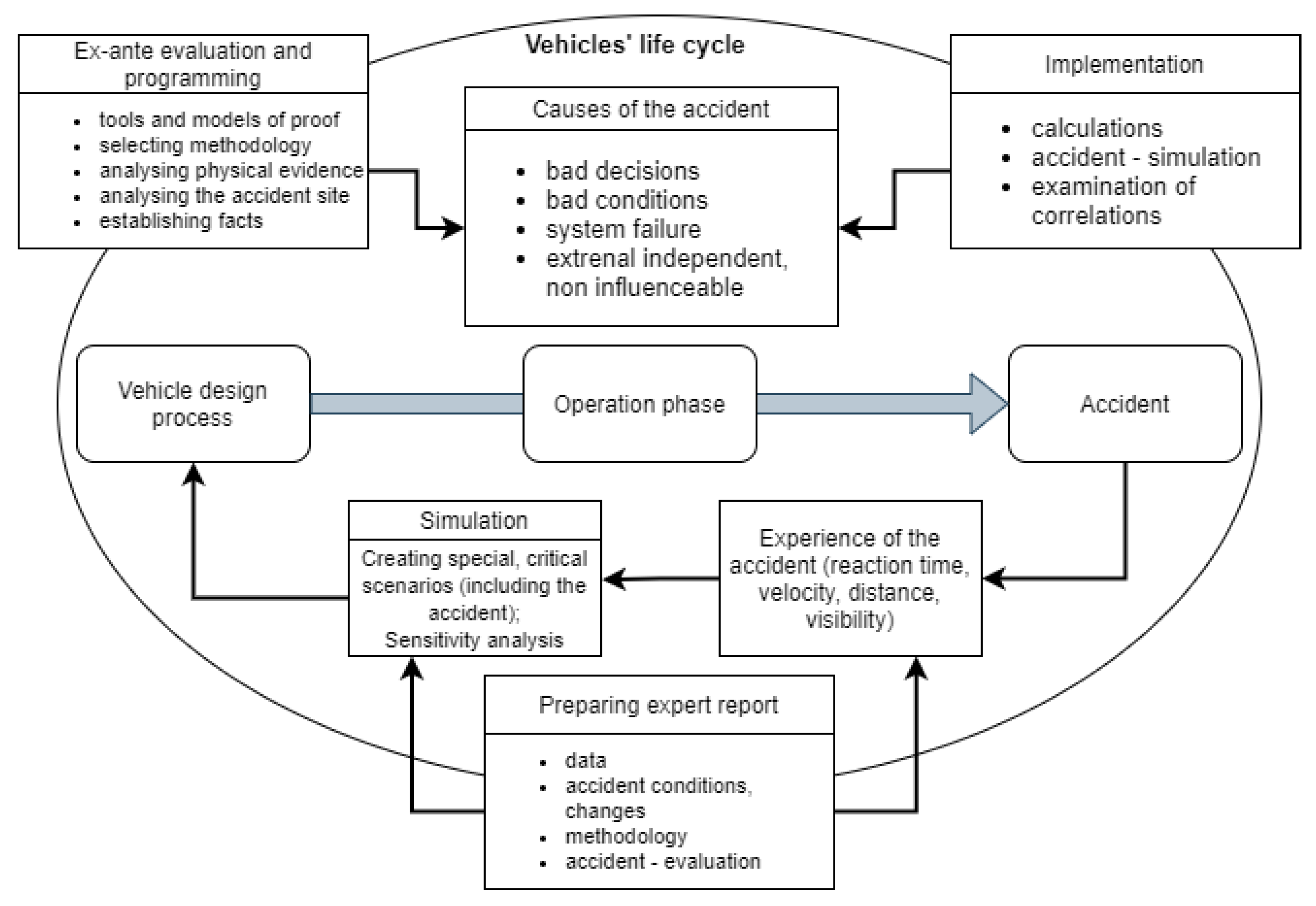
The new concept may affect the vehicle design process, as the developers can use accident data, the lessons of accidents, and create real-life-based critical scenarios. This procedure is illustrated in
Figure 1.
We call something an “accident,” it implies that no one caused it on intentionally, including the driver. The term “crash,” on the other hand, is more specific in terms of the action’s work without the unavoidable implication. In this current article, we thought about the specific crash and how to avoid them; when two objects collide (touch each other and damage occurs). The parameters of the sensitivity test and their values were chosen based on these.
The sensitivity analysis part of the methodology is further detailed in the results section. Accordingly, the accident reconstruction related to the automotive development process has to align with the V-model. The main goal of our model is to consider the causes of accidents that have already occurred already during the design phase of future vehicles. Thus, the causes of the accident are examined in the operation phase. Possible causes include bad decisions, bad conditions, system failure, external and independent factors, or non-influenceable factors. Following this, it becomes possible to conclude the accidents and construct critical and unique scenarios using the relevant factors.
The literature has validated the used data and measurements obtained from the software (IPG CarMaker and PreScan). Thus we also took the software as appropriate, which is why we got it as a basic proposition—it is considered validated software. For the simulations, we used the basic sensor settings found in the software.
As software-based exploration techniques are grounded in traditional methods of forensic experts, a brief introduction to the traditional accident analysis procedure [
33] is due. The duties of a forensic expert include professional reconnaissance and proof, all using expert tools, in the following work phases.
This study used PreScan [
34] and Car Maker simulation software to create scenarios [
35] in which a vehicle with sensors can relate to a virtual environment. Furthermore, the vehicle can respond and react to the sensors and receive data by using control algorithms that have to be implemented in Matlab Simulink [
36,
37]. We examined cases where the operation of the AEBS (Advanced Emergency Braking System) function could be linked to critical traffic situations.
In accordance with the above, the structure and parameters of the AEBS function used during the tests were uniforms. The AEBS function is controlled based on the estimated Stopping Distance (
—Equation (
1) and Time-to-Collision parameters (Equations (
3) and (
5). Accordingly, the formulas taken into account in the control method are introduced below [
38].
In the next step, we can represent the vehicle dynamics characteristics related to the modelled functions. During our research, we considered how the relevant factors influence different situations and accidents. Based on these, we can determine the speed at which the vehicle must travel to stop safely before hitting the object within a suitable braking distance. factors. In the next step, we can perform sensitivity analyses regarding the investigated parameters to evaluate the considered factors. This assessment has to be carried out during the simulation process (
Figure 1). The following formulas and calculations were applied.
Distance travelled from detection to stopping (braking distance):
where
: braking distance [m]
: vehicle speed []
: system reaction time [s]
: delay in the braking system starting to operate [s]
: the time for the full braking effect to develop [s]
: the time for the distance with full braking [s]
TTC (Time-to-Collision) can be calculated or approximated using various equations. In the case, of a following and a lead vehicle, when approaching a stationary lead vehicle, or when the lead vehicle is moving at a constant rate, Time-to-Collision is computed as follows [
39]:
If the following vehicle acceleration is assumed to be zero and if the lead vehicle is decelerating or accelerating, this lead vehicle acceleration is included in the equation as follows [
39]:
r: the range between the vehicles [m]
: relative velocity [m/s]
: velocity of the lead vehicle [m/s]
: velocity of the following vehicle [m/s]
: deceleration of the lead vehicle [m/s]
3.1. PreScan
PreScan from Model-Based Controller Design can be used for real-time tests with SiL and HiL systems. The tool allows building different traffic scenarios using a library of elements available such as actors (vehicles, animated humans, trucks, trailers), infrastructural elements (traffic signs, buildings, roads, trees), weather conditions (rain, snow, and fog), and sensors (RADARs, camera, V2X—vehicle-to-everything, ultrasonic devices) [
40].
With PreScan, a MATLAB Simulink interface is provided that allows users to design and verify the algorithms for decision-making [
41], data processing, sensor fusion, real-time collision and control [
42]. Furthermore, a 3D visualization viewer shows a visual representation of the scenario created during the simulation that can be seen from multiple points of view [
43].
Different ADAS systems were implemented, including Adaptive Cruise Control (ACC), Advanced Emergency Braking System (AEBS), Lane Change Assist (LCA), Lane Keeping Assist (LKA), Park Assist, Pedestrian Protection System (PPS), Traffic Sign Recognition (TSR).
3.2. IPG CarMaker
IPG Automotive’s main product is the vehicle simulation software CarMaker. This software enables real-time functional and performance testing using virtual vehicle prototypes. In the CarMaker product family, chassis control systems, steering systems and suspension design, and ready-made virtual prototypes from the software can be developed. As an actuator, the steering system is also important for the development of ADAS functions. One of the advantages of CarMaker is that there are basic fixed models (vehicle, suspension, tires, etc.) and the number of bodies and the degrees of freedom (DOF) between them is already defined [
44].
The animation of the simulation can be seen in IPGMovie while running the simulation. The IPG Control tool can use the results to plot various simulation diagrams. The tool is able to model traffic environments, connect with control systems, and visualize simulation results, which are specifically considered. A set of scenarios are realized to evaluate the tool’s strengths concerning the features considered. In this simulation software, critical scenarios can be created, using accident data, and the experiences of the accident [
45].
3.3. Investigated Accident Scenarios
This section explains how PreScan and CarMaker created the desired scenarios. It demonstrates the development of a traffic environment and the simulation of the resulting design. In our experience, both software programs are suitable for modelling driving assistance systems with different levels of automation and taking into account special vehicle dynamics aspects [
46]. The PreScan software provides a more detailed design environment for examining vehicle control logic, while CarMaker can be used more widely to analyse vehicle dynamics parameters.
In order to present the new methodology, accidents that have occurred due to the failure of highly automated functions and are well documented were selected, and thus the accident process and causes are available detail.
The preliminary assessment found that the functions supporting the automated driving system played a larger role in the control system for the examined first two accident scenarios, so they were modelled in the PreScan software. For the third and fourth accident scenarios, the preliminary evaluation found that the characteristics of the relationship between the vehicle and the environment played a more significant role, so these were modelled in the CarMaker software.
3.3.1. Reconstruction of the First Scenario in PreScan
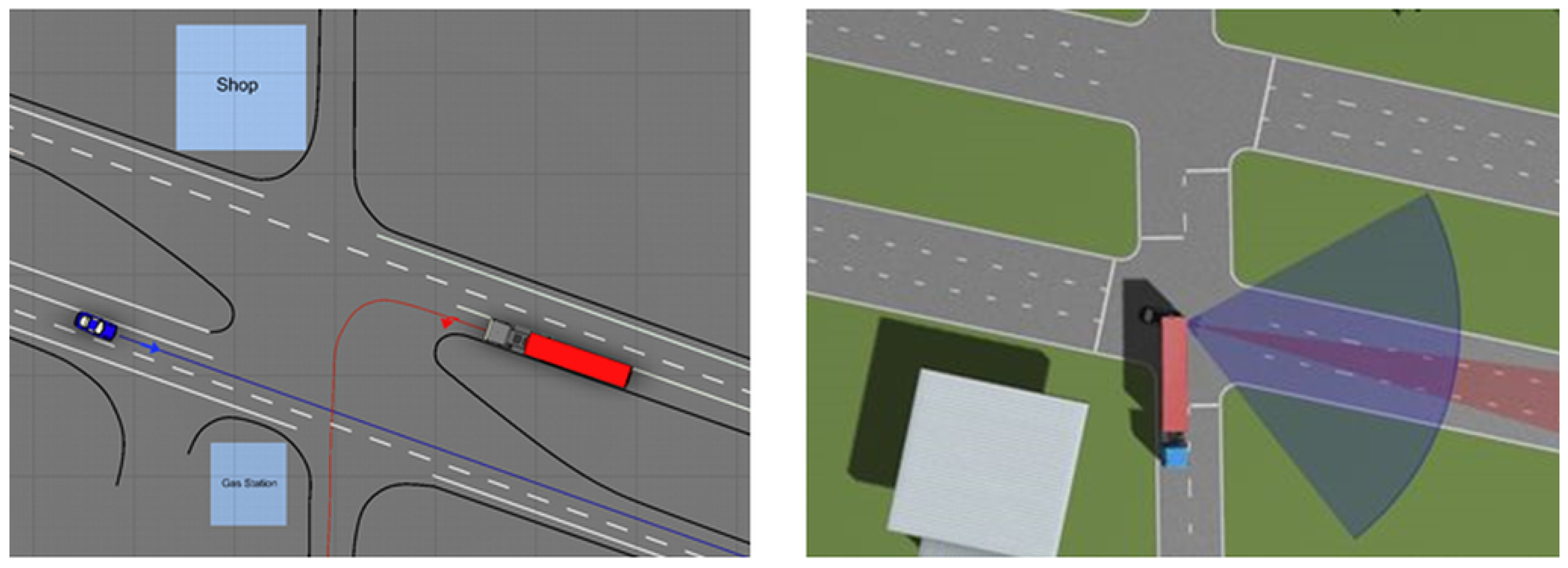
The first accident occurred in May 2016 in Florida, near Williston [
47]. A Tesla Model S driving by autopilot on a highway to the east crashed into a semi-trailer [
48]. The truck, heading west, was making a left turn off the road in front of the Tesla. The Tesla did not stop, but hit the trailer and travelled under it. The Tesla driver died. The accident is illustrated in
Figure 2.
Two variables were chosen for the sensitivity analysis [
49]. This is the variable of maximum braking pressure during partial braking and the roll friction coefficient. We chose these parameters based on accident situations analysed in reality. After the selection, we also compared the factors used in the test method with the capabilities of the simulation software. Partial braking is a phase of the Advanced Emergency Braking System (AEBS), when the system brakings partially. Partial braking only requires information from a long-range RADAR sensor (LRR).
3.3.2. Reconstruction of the Second Scenario in PreScan
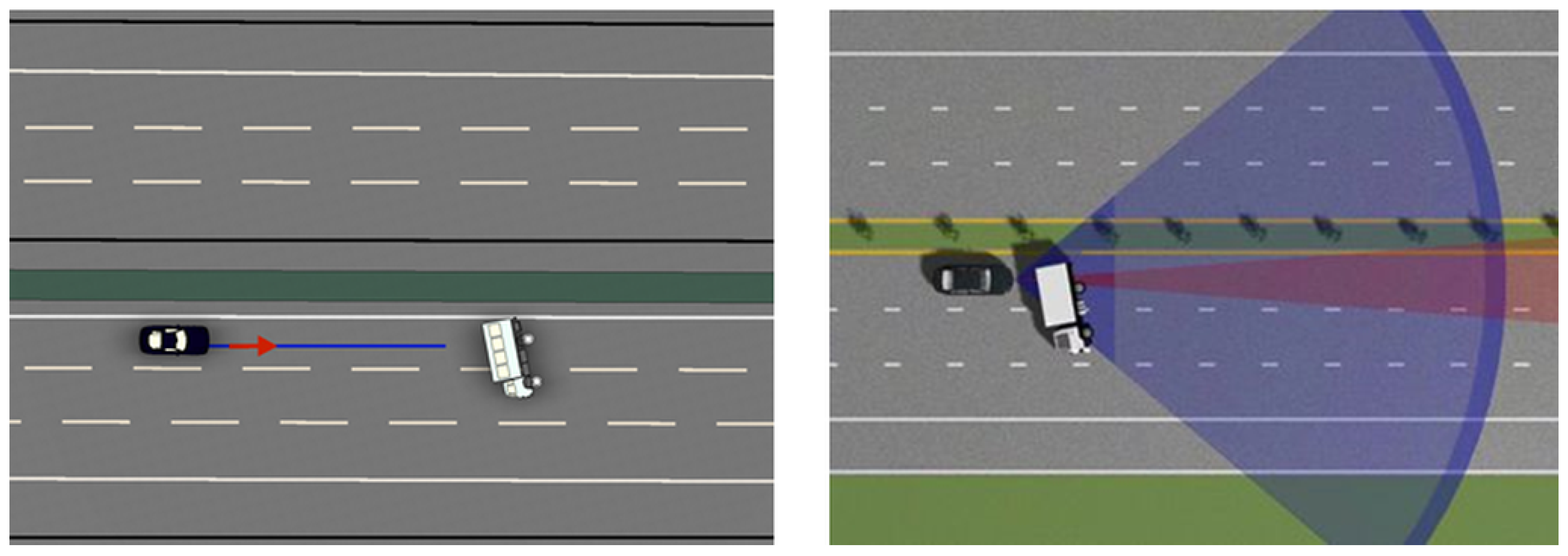
The next accident happened in June 2020 in Taiwan [
50]. The autopilot function was turned on when the Tesla Model 3 travelled around 110 kilometres per hour along Sun Yat-Sen Highway [
51], near Chiayi City, and crashed into an overturned white truck
Figure 3. That obstacle did not move and was quite extensive.
The best decision will be to change variables related to the “Time-to-collision” (TTC) parameter of AEBS. There are three parameters of TTC. The first one is the driver’s warning before the predicted collision. By default, it is 2.6 s, but this parameter will not be used in our case with autopilot. The next is the start of partial braking, for which the default is 1.6 s. The last is full braking, 0.6 s before the collision. It should be mentioned that fully automated braking activates only when both sensors detect the colliding object. Meanwhile, partial braking needs information only from LRR [
52].
After testing with default variables, the ego-vehicle crashed at a speed of 61 km/h.
3.3.3. Reconstruction of the Third Scenario in IPG CarMaker
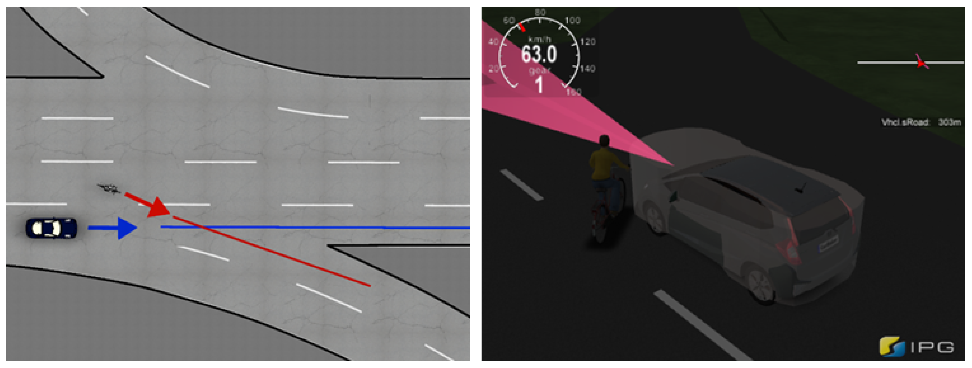
An accident occurred in Tempe, Arizona, in March 2018 [
53], when an Uber car failed to identify a pedestrian, struck, and killed Elaine Herzberg, while the car was working in computer control mode (
Figure 4). The CarMaker was used to build the simulation [
54]. As an Uber car, CarMaker used a Honda, which was parameterized by default. The posted speed limit was 70 km/h.
A CarMaker project consists of a road model, an ego car model, and a traffic model that includes a target pedestrian with a bicycle and its movements. CarMaker uses a GUI (Graphical User Interface) to navigate between the specifications of the different models. Autonomous emergency braking (AEB) will be implemented within this TestRun1.
Figure 4 shows the collision of a car and a bicyclist with the parameters specified. Due to the limited possibilities of the CarMaker, a cyclist was used instead of a pedestrian with a bicycle. We have to mention that the IPG CarMaker defines the field of view based on the horizontal width and vertical height of the visible image area in the case of a specific working distance defined by the range parameter.
After the configuration of the road and selecting an ego vehicle, the scheme of the ego vehicle needs to be defined. Firstly, the start velocity and the number of gears should be given. For this scenario, the start velocity is 70 km/h, and the fifth gear is active at the beginning of the simulation. The primary manoeuvre of the vehicle is longitudinal dynamic with a duration of 60 s; the speed within this manoeuvre is also 70 km/h.
The sensor and controller are attached to the vehicle to mimic the Autonomous Emergency Braking system. The AEB system decelerates the vehicle safely to the velocity of the target object ahead by controller-defined longitudinal control with a referenced sensor, a camera. The sensitivity analysis [
55] presents the implementation of a scenario with two variables that affect the result of the simulation. As the first value was taken from the field of the view of the camera equipped on an ego vehicle, the second value is altering the speed of the pedestrian with a bicycle. The car with self-driving mode was initially set to 70 km/h velocity. The crash was during the night, so the assumed field of view of the camera was small. The camera parameters during the manoeuvre that lead to the crash and changed values can affect the simulation result. The speed of the pedestrian with the bicycle was 1.4 m/s.
In
Figure 4, due to the fact that the camera field of view (horizontal and vertical) was increased from 10 m/10 m, thus the cyclist was detected, and the collision between the car and the cyclist was avoided. The IPG Movie showed how the camera caught the cyclist; the AEB was triggered (in the simulation the longitudinal control, AEB was used for the controller) and brakingd the car 5 m away from the cyclist. The range between the objects was 20 m. In the simulation, the field of view parameters (horizontal and vertical) were changed to 45 m/45 m. When the field of view was 45 m, the collision was avoided.
3.3.4. Reconstruction of the Fourth Scenario in CarMaker
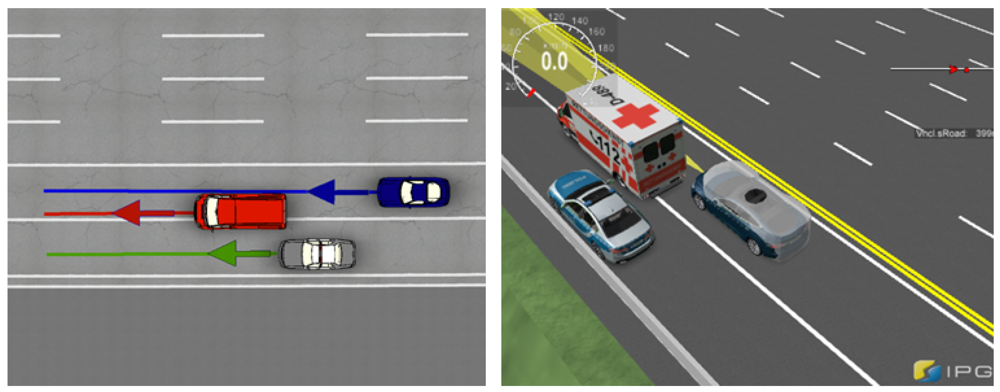
For the fourth reconstruction, the accident was in Culver City, California, in January 2018. The crash involved a Tesla Model S P85 and a Culver City Fire Department 2006 Seagrave Fire Truck in the high-occupancy vehicle lane of southbound Interstate 405 [
56]. The accident did not result in any injuries, the situation was used because of the Tesla could not recognize the situation well. The simulation was prepared in CarMaker. As the Tesla car in CarMaker was used, the Tesla S was parametrized by default. The posted speed limit was 70 km/h.
The CarMaker project consists of a road model, an ego car model, and a traffic model that includes a lead vehicle, an ambulance car (in a real-life Fire Truck), and their movements. CarMaker uses a GUI to navigate between specifications of the different models. The adaptive cruise control system (ACC) is implemented within this TestRun.
For this scenario, the ego vehicle velocity is 100 km/h, and the lead vehicle velocity is 34 km/h, and the fifth gear is active at the beginning of the simulation. An advanced driver assistance system—ACC Controller was added to the ego vehicle’s default parameters, and the ego vehicle’s decreased velocity due to ACC was 34 km/h. The ACC device controls the longitudinal acceleration of the vehicle by changing the position of the braking and gas pedal. If there is a relevant target detected, the distance will be controlled.
The manoeuvre of the ego car is to approach a slower vehicle with activated Adaptive Cruise Control and to change to set-up speed after the lead vehicle sheers out from the HOV (high-occupancy vehicle). The reference sensor for detecting targets is a RADAR. A crash detection system is also applied in the simulation.
The sensitivity analysis depicts the execution of the scenario with two variables that influence the simulation outcome. The first value was the increasing distance before the cutout manoeuvre of the lead vehicle in front of the ego car from the HOV line to the right; the second value was altering the speed of the lead vehicle.
The speed of the car with self-driving mode was initially set to 100 km/h. According to NTSB (National Transportation Safety Board) [
56], 3 to 4 s before the crash, the lead vehicle (T01) changed lanes to the right. That movement is referred to as a “cutout scenario” [
57].
Figure 5 shows the moment of collision of the ego vehicle and a truck stopped in the center of two lanes. Because of the small distance for the deceleration of the ego vehicle, even though the RADAR detected the static object, the collision happened.
Figure 5 illustrated the detection of the truck by the RADAR, thus the ego vehicle brakingd, so the collision was avoided. The
distance between the truck and the start of the cutout manoeuvre of the lead vehicle (T01) was increased from 15 m to 20 m. The ego car decreased the speed to 0 km/h.
4. Results and Discussion
4.1. First Scenario
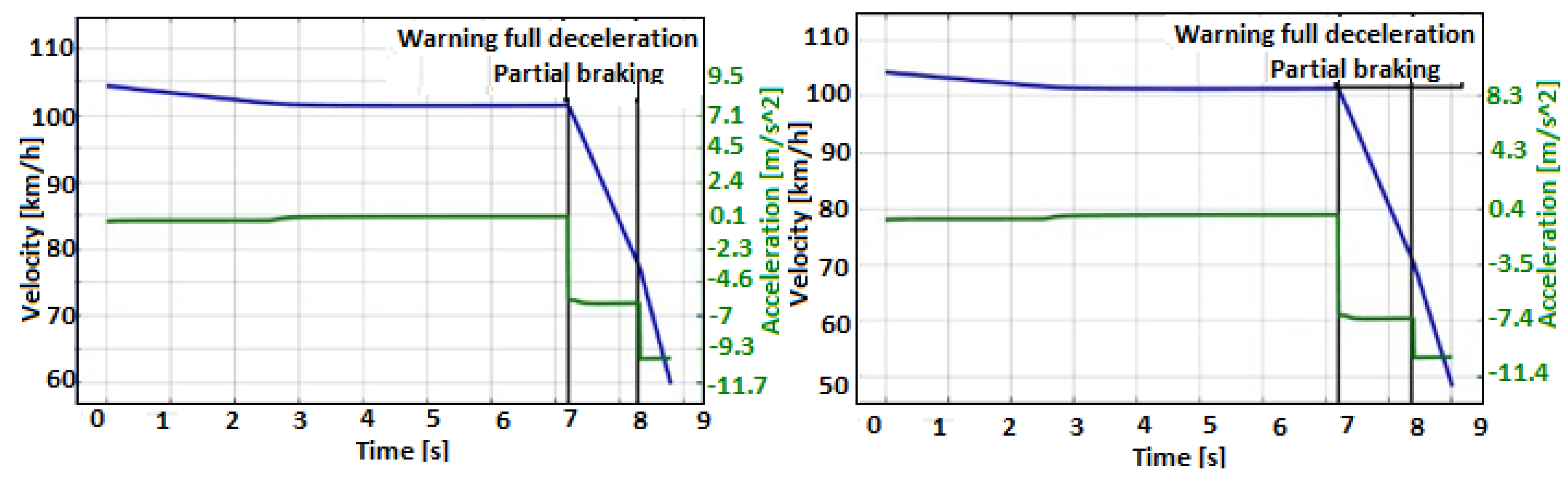
To prevent this accident, the value of maximum braking pressure was increased smoothly for partial braking. After several experiments with various values, the crash was avoided at 60%. Below, in
Figure 6, the ego vehicle speed profiles are shown with 50% and 60% values. The difference in the partial braking section is visible when comparing the two profiles due to the high braking pressure.
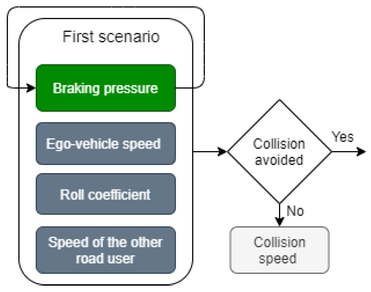
To investigate the scenarios comparably, we applied the following schematic form. This makes it possible, on the one hand, to describe the four scenarios and, on the other hand, to present sensitivity analysis through a schematic flow chart as well.
In the first scenario, we considered braking pressure, ego-vehicle speed, roll coefficient and speed of the other road users to reconstruct the analysed crash. We modified the braking pressure (indicated by green background) during the evaluation to investigate the impact of this factor on the outcomes of the crash (
Figure 7).
The collision was avoided only after increasing the value of the maximum braking pressure to 60%.
Table 1. shows a comparison of the effect of braking pressure during partial braking.
After the reconstruction of the crash in PreScan, the sensitivity analysis was provided. The first variable, which was changed to prevent the collision, was braking pressure during the partial braking. It was raised from 40% to 60% of full braking. According to
Table 1, on the default value, the crash happened at a speed of 69 km/h. After this, partial braking pressure was increased to 50%. This time the collision happened at 60 km/h. Finally, at 60%, the crash was avoided.
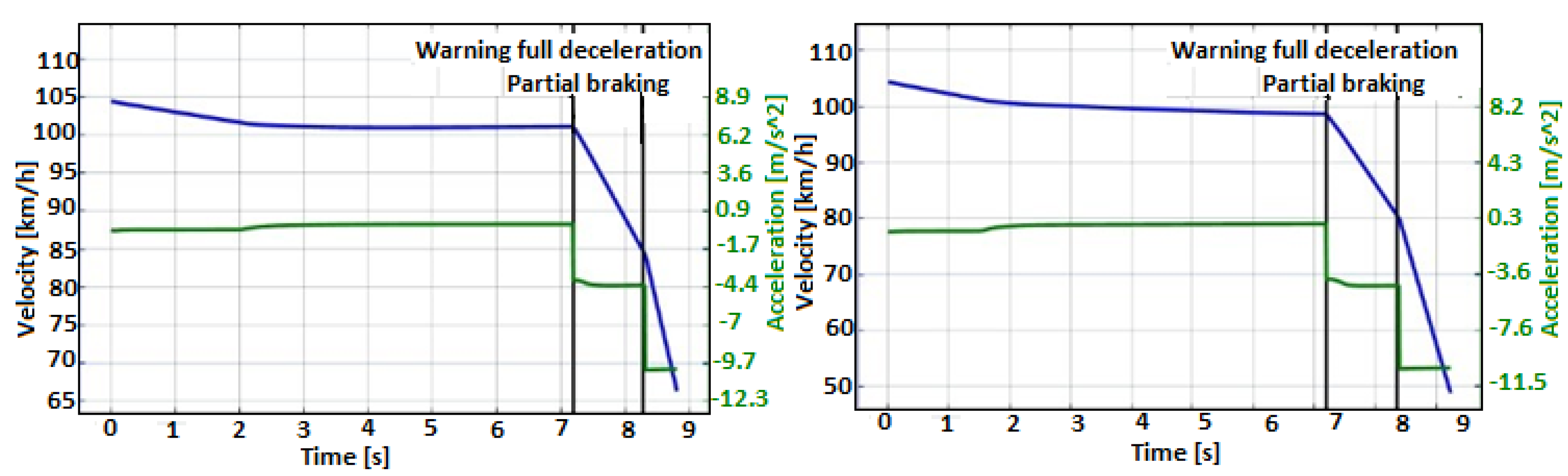
The next parameter, which affects the experiment, is the roll friction coefficient. The default value is 0.01, and similarly to the previous parameter, this coefficient was varied smoothly until the accident was prevented. Below,
Figure 8 presents the speed profiles of the ego vehicle with modified values of roll friction coefficient. The main difference is in the partial braking section. By increasing the rolling friction coefficient, the car slows down more efficiently.
The rolling friction coefficient variable was varied until collision was avoided. A positive result was obtained at a value of 0.04. Below,
Table 2. shows the results of changing the value of the roll friction coefficient.
The larger the rolling friction coefficient is, the easier it is to slow down. Due to this fact,
Table 2 shows that collision speed decreases while the coefficient rises. The collision was avoided when the value equalled 0.04.
4.2. Second Scenario
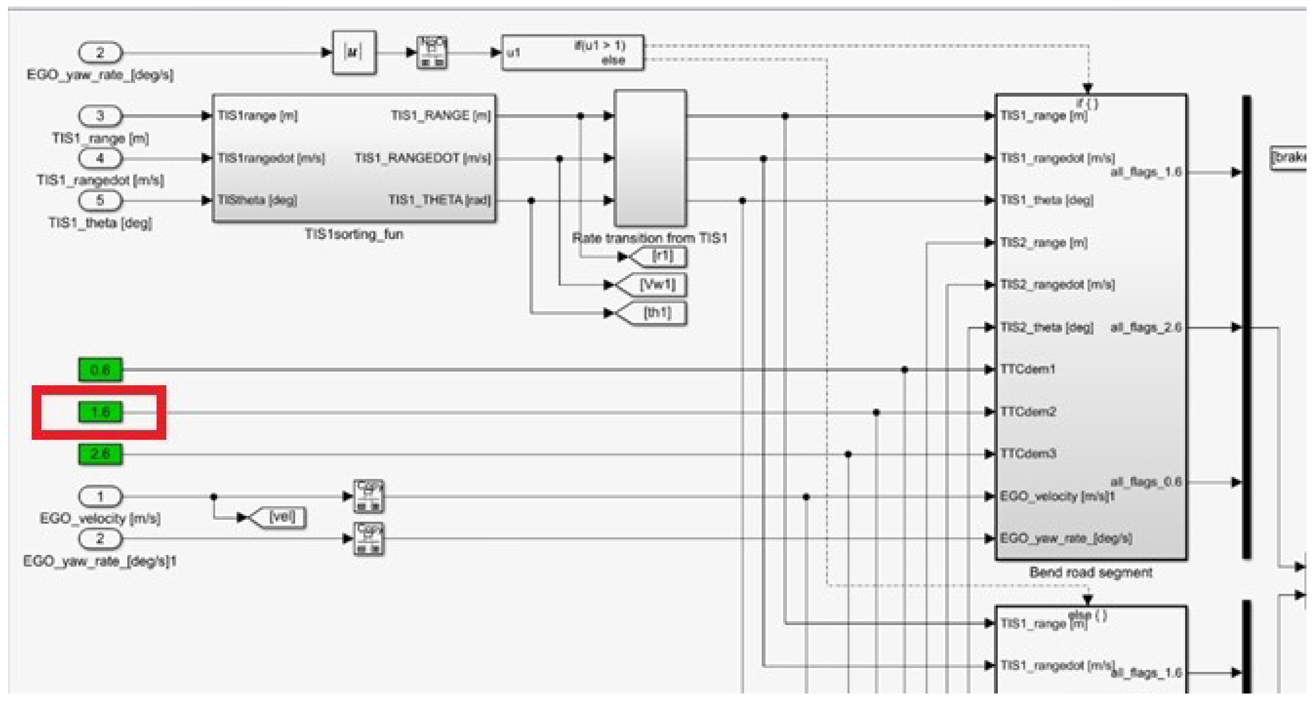
The first variable to be changed is the starting of the partial braking phase [
58]. The parameters used during the simulations are also shown in a block diagram; this diagram can be modified in the software using Simulink (
Figure 9 and
Figure 10). For that, the TTC related to this parameter will be edited (
Figure 9) until collision avoidance; the red square represents the parameters of TTC, and the default value is 0.6 s before the predicted collision. After running the experiment several times, a satisfactory result was obtained.
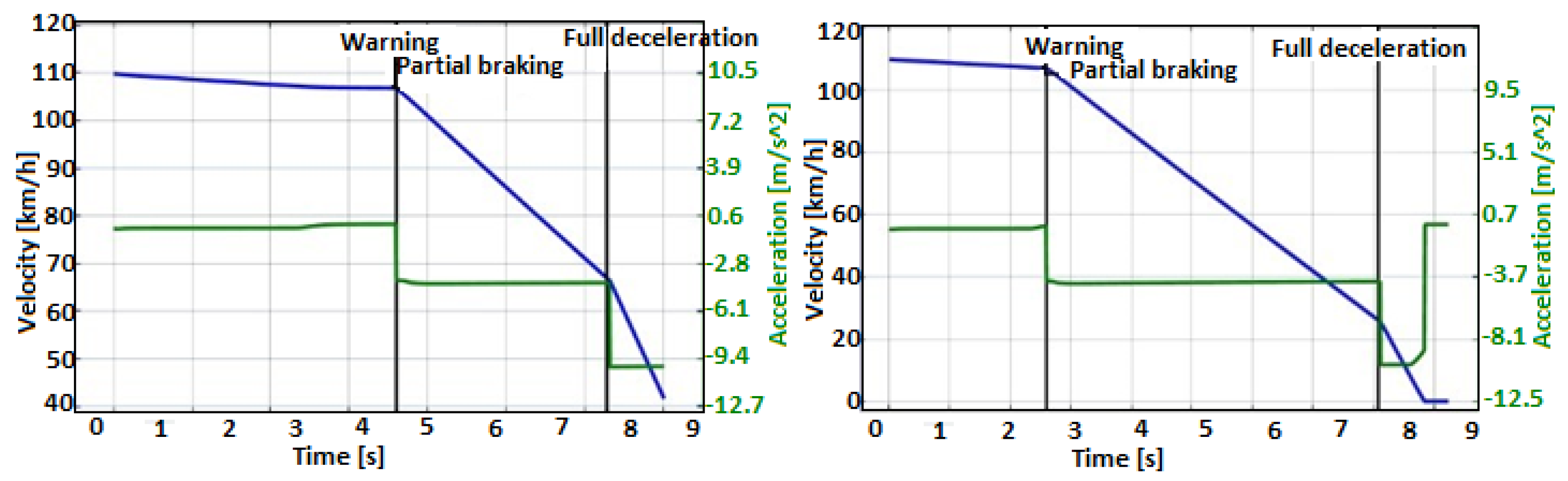
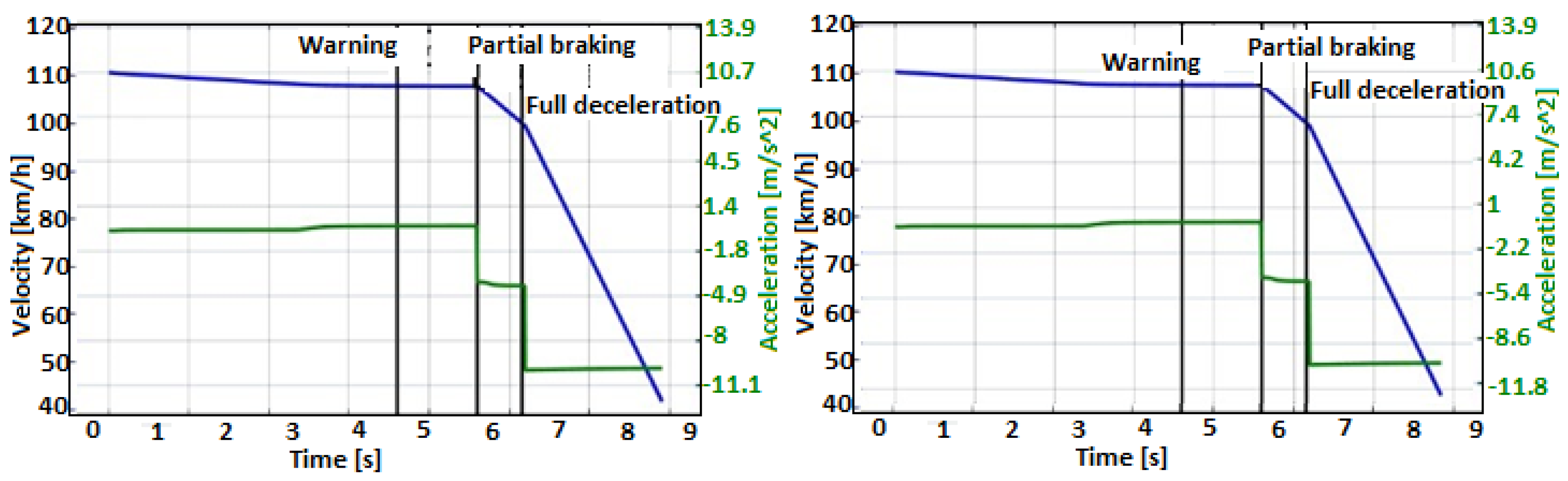
Figure 11 shows the speed profiles when TTC equalled 2.6 and 3.6 s, respectively. The main difference between them is that the higher the value of the TTC, the sooner the car starts the partial braking phase. The figure shows that the crash can be avoided when TTC is 3.6 s.
Table 3 presents the comparison of TTC values.
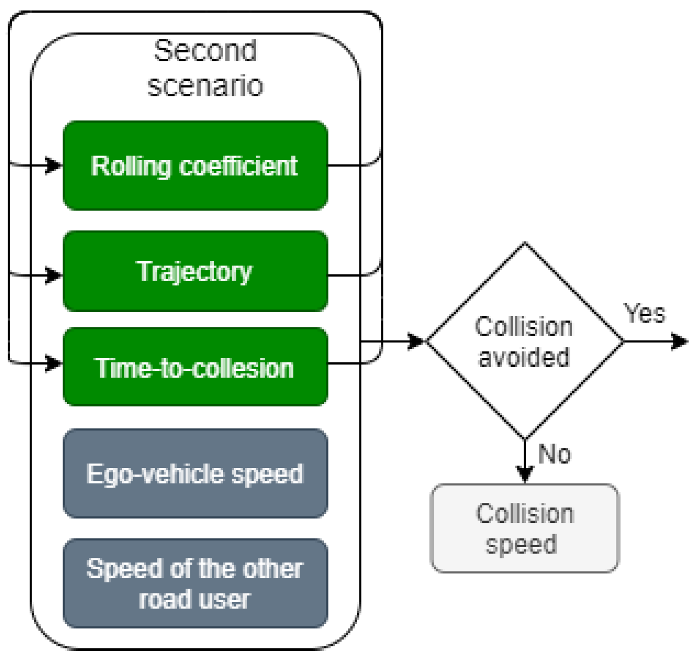
In the second scenario, we considered ego-vehicle speed, rolling coefficient, Time-to-Collision, trajectory and speed of the other road users to reconstruct the analysed crash. We modified the roll coefficient, trajectory and the TTC (indicated by green background) during the evaluation to investigate the impact of this factor on the outcomes of the crash (
Figure 12).
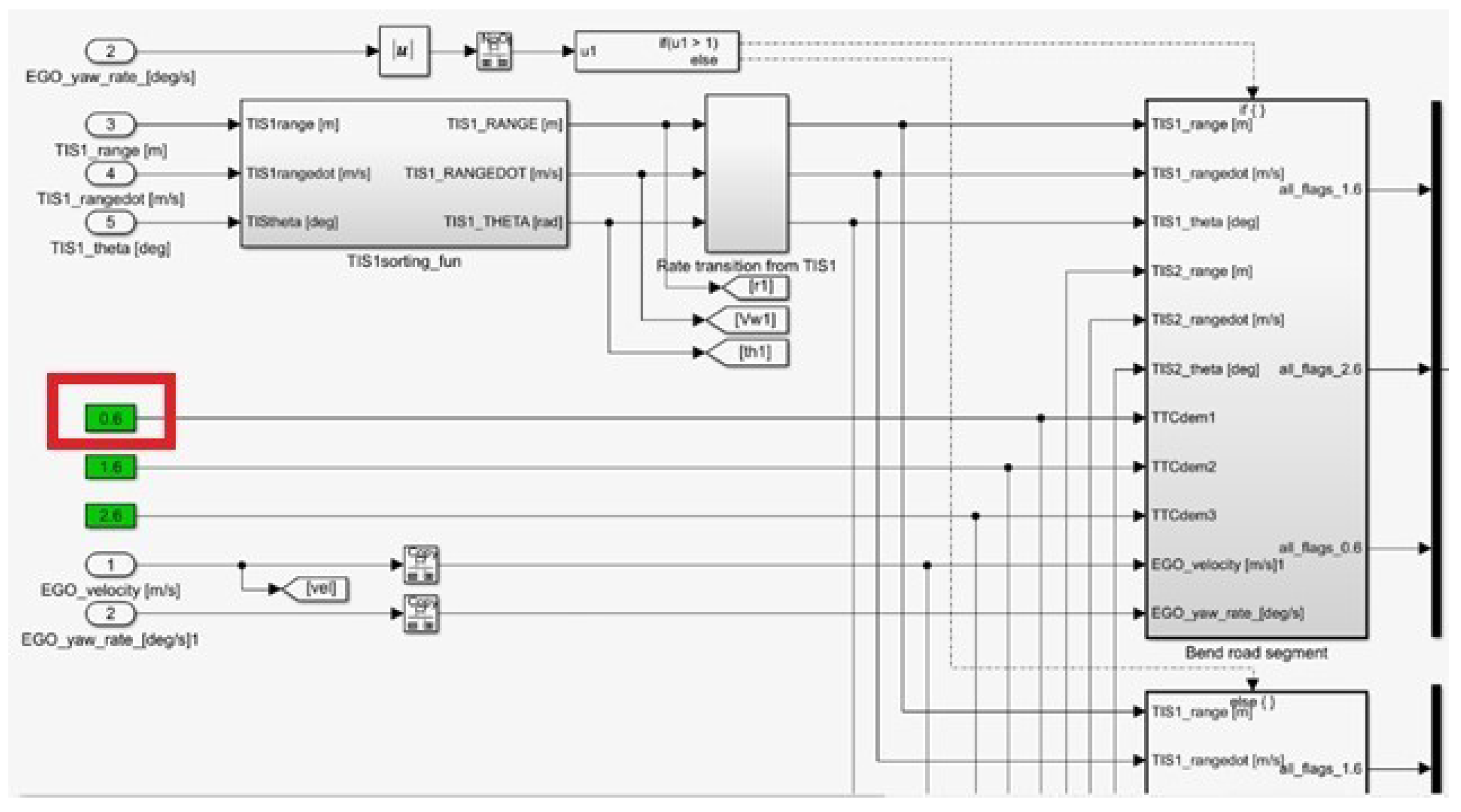
There is another TTC parameter (
Figure 10), but this one starts full braking. The default value is 0.6 s before the predicted collision. This variable is changed until the accident is eliminated.
The variable was changed three times—1.1 and 2.1 (
Figure 13). However, all values gave unsatisfactory results. The collision speed is stuck at 38 km/h, because full braking needs information from two sensors. Only changing the parameter from 0.6 to 1.1 gave better results, but it is impossible to avoid the crash.
Table 3 shows the comparison between different values of TTC.
As in the previous scene, the AEBS block was used. First, the trajectory of the ego-vehicle was shifted. In the first step, it was shifted to by 5 cm, but the crash happened at a speed of 59 km/h. Then the trajectory was shifted by 10 cm, and the car was stopped 8 m before the human (see:
Table 4). The results are presented in
Table 3. The second variable is the shifting of the sensors. With a shift of 5 cm, exactly the same effect was obtained: the car hit the driver at a speed of 59 km/h. As expected, the accident was prevented with a shift of 10 cm, and the car stopped 8 m in front of the pedestrian.
Since the changing of the TTC of full braking did not give a good result, it should be checked what happens if both previous parameters are changed.
After adding 0.5 s to each parameter, the collision speed was 27 km/h. Then adding additional 0.5 s, the crash was avoided. The car stopped around 3 m before the collision,
Table 5 shows the results.
As in the first scene, the car’s camera is blinded by the sun. In this experiment, TTCs related to partial braking and full braking were configured. The first was the TTC which starts the partial braking phase.
Table 4 shows the results of it. The value was increased to 0.5 until crash prevention. The higher the value of the TTC, the earlier the phase of partial braking begins. When the variable was equal to 3.6 s, the crash was avoided. The second TTC to be changed was the TTC of full braking. Full braking requires information from LLR and SRR. The default value is 0.6 s, and the collision speed is 64 km/h. After raising the TTC to 1.1, the speed of collision became 38 km/h. However, with a further increase, the result remains the same, and the car crashes. The sensor range is limited, and it is impossible to receive the information for the SRR earlier. The default values of both TTCs are 0.6 (full braking) and 1.6 (partial braking), see
Table 5. By default, the car crashes at 64 km/h. After raising the TTC to 0.5 s, the car crashed at 27 km/h, significantly decreasing. Then, at values 1.6 and 2.6, the crash was avoided.
4.3. Third Scenario
In this scenario, the cyclist’s speed was changed; the speed at which the collision will be avoided is 1.4 m/s. The IPG Control tool shows selected output quantities in real time, and the results can be plotted.
All of the simulation experiments were performed using changeable external parameters, such as the distance between the lead vehicle and the ego vehicle, the distance before the cutoff manoeuvre, and the velocity of traffic objects other than the ego car.
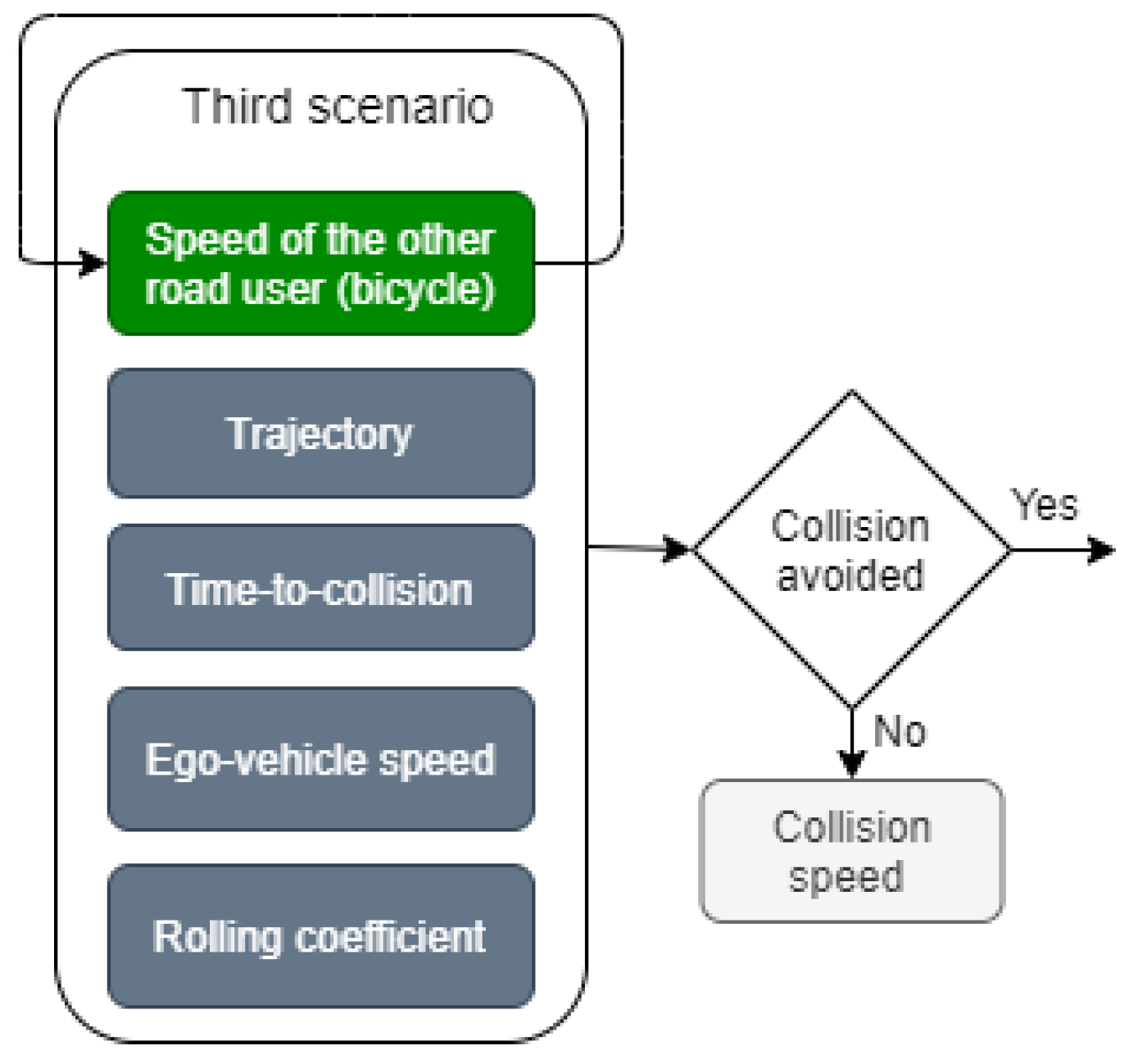
In the third scenario, we considered ego-vehicle speed, roll coefficient, Time-to-Collision, trajectory and speed of the other road users to reconstruct the analysed crash. We modified the speed of the other road user—bicycle speed—(indicated by green background) during the evaluation to investigate the impact of this factor on the outcomes of the crash (
Figure 14).
As mentioned in
Section 3.3.3, the simulation of scenario TestRun1 involved the ego vehicle with an autonomous driving assistance system [
59], including a longitudinal controller, the autonomous emergency braking system, and a camera. Since the accident described in
Section 3.3.3 took place in the dark, the field of view of the camera was narrow, considering the effects of bad weather on the camera in real life. Even when the vehicle was equipped with a camera that does not work well in bad weather and RADAR and LiDAR systems, which have low resolution, the sensor system could not recognize an object in poor lighting.
The camera’s field of view was enlarged enough to avoid collision during the sensitivity analysis. When the camera angle is increased, the ADAS system detects a pedestrian with a bicycle, and the autonomous emergency braking system is activated. The second parameter for comparison was the speed of the pedestrian with a bike; when the speed of the cyclist was reduced to 1.4 m/s, the car had time to pass and did not collide with a pedestrian. When the speed of a pedestrian with a bicycle increased to 1.7 m/s, the pedestrian got into the limited angle of view of the camera, and the emergency braking system was activated, which prevented the accident. According to the sensitivity analysis data, changing only one parameter could affect the outcome of incidents; in this case, it was possible to test an autonomous car in a place more isolated from pedestrians and in an area equipped with sufficient lighting.
Figure 15 and
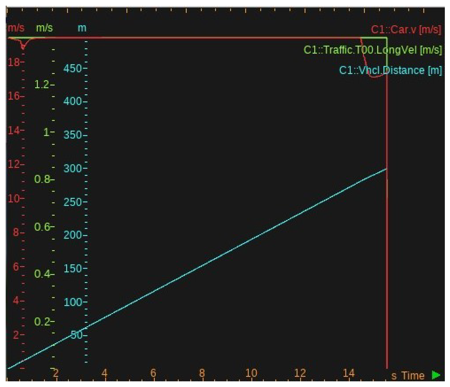
Figure 16 shows a graph of the movement of the car and the cyclist with the parameters specified; which means the velocities are 1.4 m/s (collision happened), 1.3 m/s (collision avoided), 1.7 m/s (collision avoided). As seen from the chart, a collision will occur when the vehicle reaches a distance of 300 m, and the simulation will stop. The used sensor is a camera.
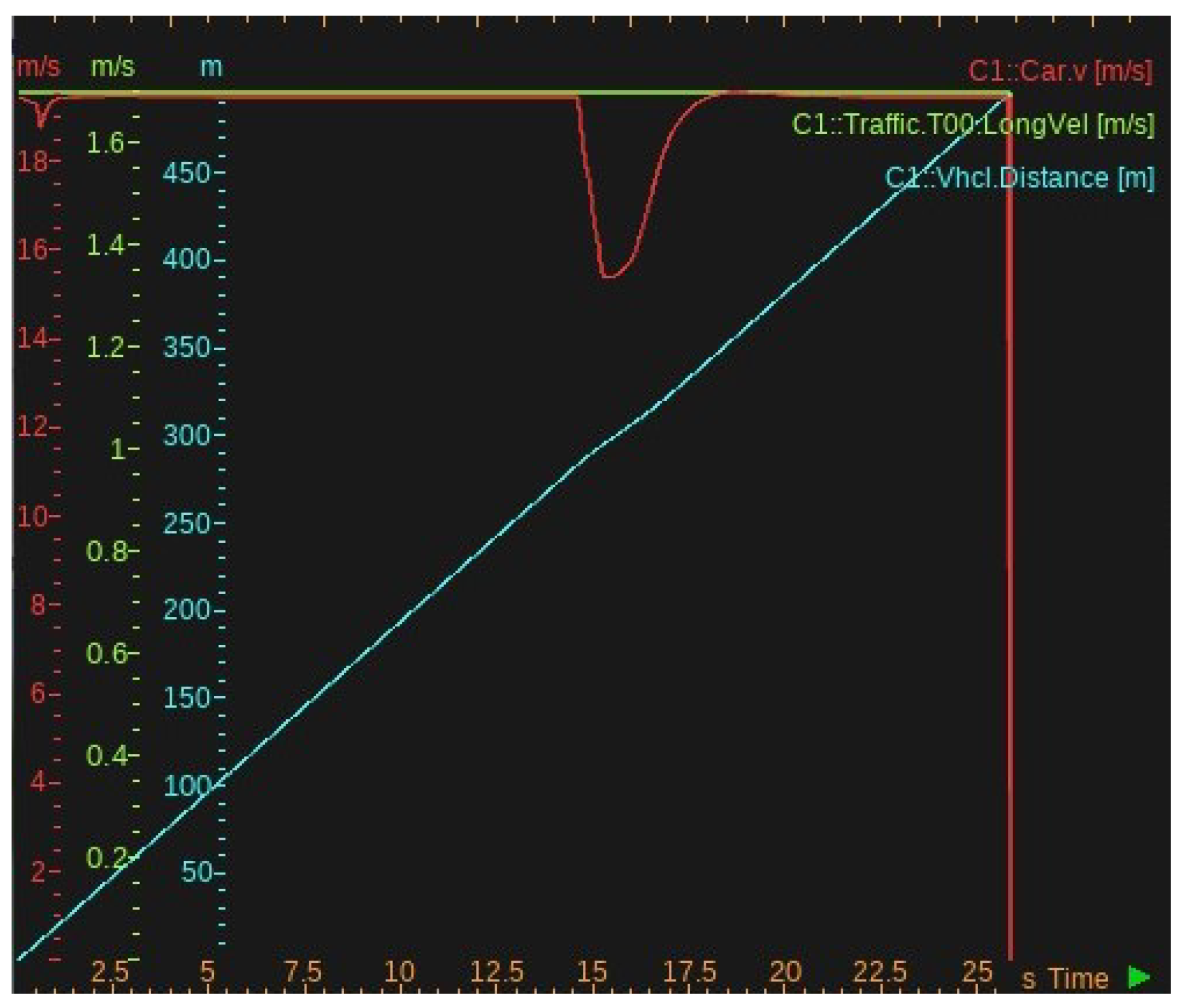
Figure 15 and
Figure 16 shows a graph with reduced cyclist speed. Due to the reduced speed of the cyclist, the car will go through the intersection faster, and there will be no collision. The simulation ends when the ego vehicle reaches the end of the testing highway—500 m. The adaptive cruise control system (ACC) will be implemented within this third scenario.
Figure 15 and
Figure 16 displays a graph with an increased speed of the cyclist, equal to 1.7 m/s; according to the chart, the car will notice the cyclist, although the camera has a small field of view, and the car will break and go on after the cyclist passes the intersection. At the 15th second, the speed of the vehicle decreases rapidly. The velocities of the ego vehicle and the bicyclist are 70 km/h and 1.4 m/s, respectively, see
Figure 15 and
Figure 16.
Figure 15 and
Figure 16 displays a graph with an increased speed of the cyclist equal to 1.7 m/s; according to the chart, the car will notice the cyclist, although it has a small field of view of the camera, and will brake and go further after the cyclist passes the intersection.
However, we must be careful with evaluating the speed of vulnerable road users since, in some cases, the results can suggest that the increased speed of cyclists could avoid crashes. This conclusion would be wrong; therefore, we must pay serious attention to analysing the outcomes of tested scenarios. Accordingly, the outcomes of the scenarios depend on when the cyclist starts to cross the road to arrive at the conflict point.
4.4. Fourth Scenario
The second parameter for the sensitivity analysis is the reduced speed of the lead vehicle. The speed of the leading car at the time of this accident was 34 km/h; for comparison, the speed will decrease to 28 km/h. The simulation of this accident showed that starting from this speed and less, Tesla S will have time to stop in front of the truck and avoid a collision.
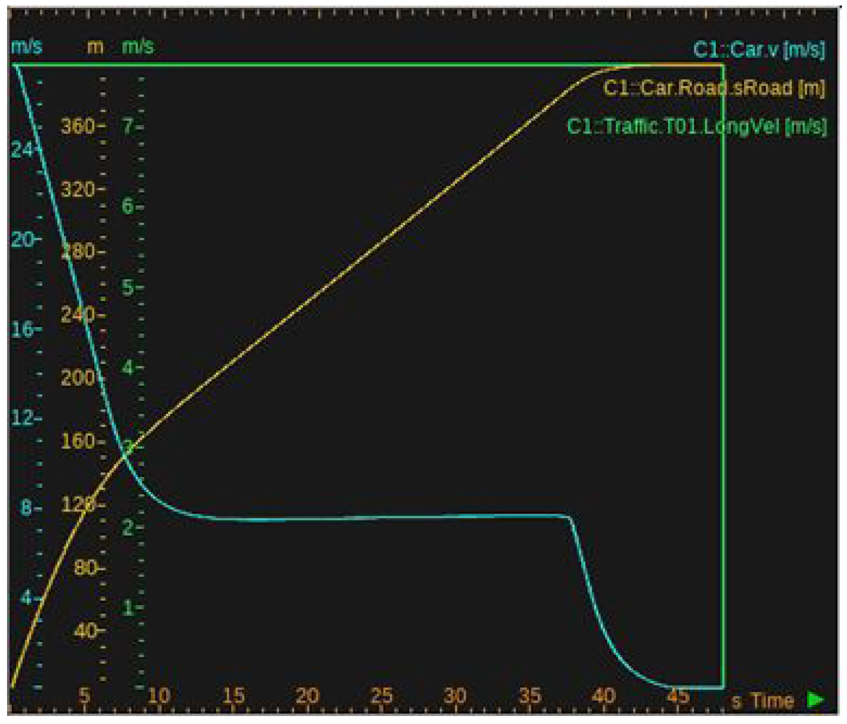
Figure 17 shows a collision-avoidance visualisation. The adaptive cruise control system (ACC) will be implemented within this scenario. The sensor is a RADAR. The minimal distance before the collision object is 10 m. The distance between the truck and the start of the cutoff manoeuvre of the lead vehicle is 15 m.
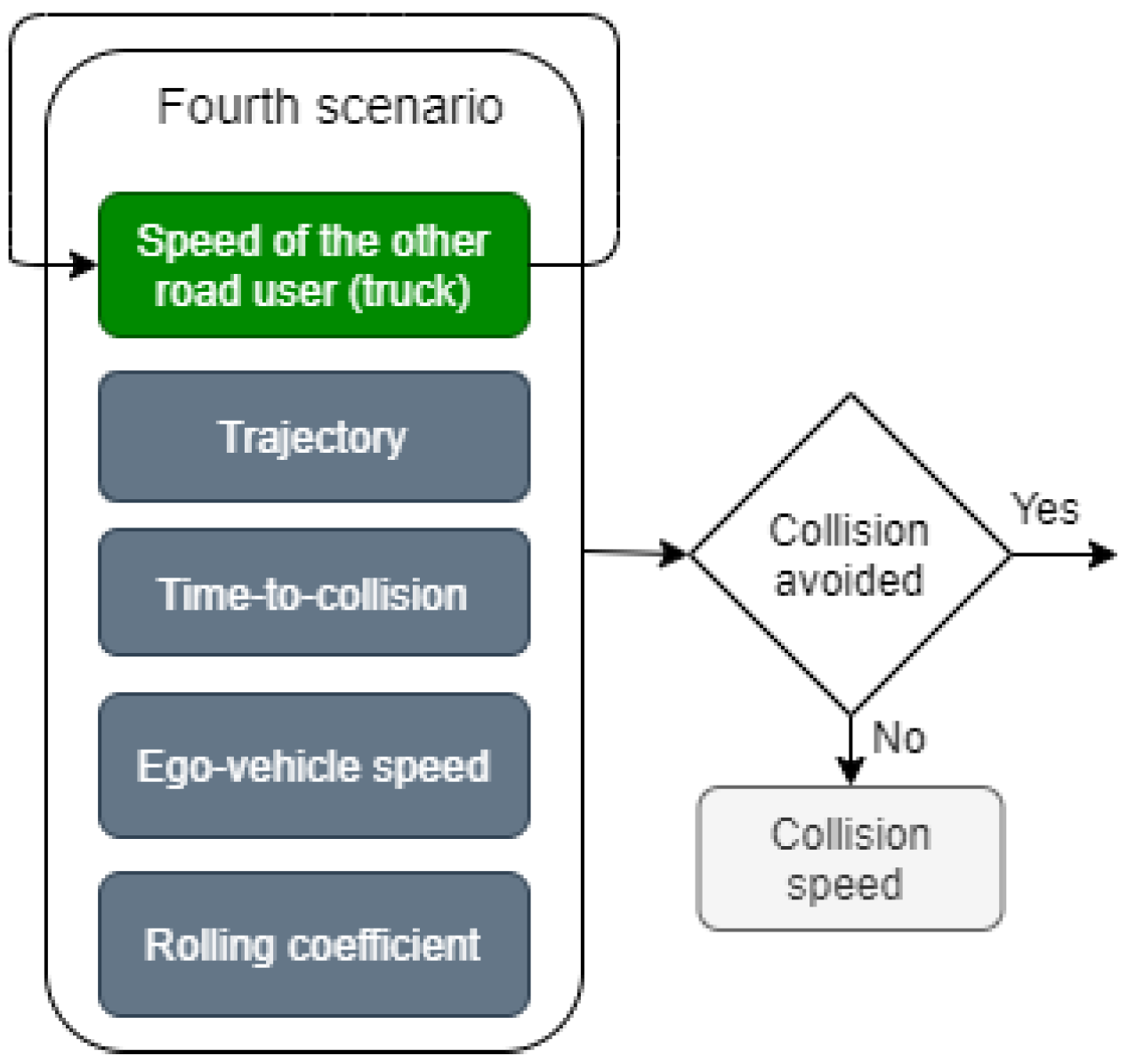
In the fourth scenario, we considered ego-vehicle speed, roll coefficient, Time-to-Collision, trajectory and speed of the other road users to reconstruct the analysed crash. We modified the speed of the other road user—truck speed—(indicated by green background) during the evaluation to investigate the impact of this factor on the outcomes of the crash (
Figure 18).
Figure 17 displays a plot of vehicle speeds and the distance from the start of the simulation till the end. As seen from the chart, the ego vehicle starts to decelerate from 380 m when the lead vehicle (T01) turns to the right. Tesla S stops before the truck and avoids the collision.
As discussed in
Section 3.3.4, participants of this accident were the leading car before the Tesla, a fire truck, and a police vehicle. During the manoeuvre, Tesla followed several leading vehicles with an activated ACC system. When the last leading car turned to the right 3–4 s before the collision, the autonomous vehicle system did not detect that the truck in front of it was not moving. In this simulation, the first changing parameter was the increased distance between the start of the lane departure manoeuvre of the leading car and the fire truck. The distance increases; therefore, the time for Tesla to detect a static object and avoid crashes by emergency braking increases. The second parameter is the speed of the leading car. The reduction of velocity leads to the decrease of the ego vehicle’s speed accordingly, owing to the ACC system. Considering the results after the analysis, it can be assumed that with the autonomous control of the car, there should be restrictions on the maximum speed in order to have time to braking and avoid crashes. Autonomous car drivers rely heavily on intelligent systems and lose their vigilance.
5. Conclusions
Our research aimed to explore a comprehensive analytical framework of highly automated vehicle accidents to identify critical scenarios for highly automated vehicles’ test and validation processes. As the first step, it is necessary to choose accidents that can be fully or partly explained by the malfunction of intra-vehicular E/E systems or by the decision-making/execution layer’s failed operation.
Following this, we need to identify the proper reconstruction tool related to the given accident. The adequate decision depends on the most significant causal factor of the accident. According to our experiences, some simulation environments can more efficiently be applied to describe the operation of the decision-making/execution layers’ processes, including control blocks and dynamic parameters (e.g., PreScan). At the same time, some of the applications have more detailed features to model sensor operation or the interaction of the vehicular system and the external environment (e.g., IPG CarMaker).
Of course, to draw holistic conclusions, we need to extend the analysis to have a statistically significant sample size. However, we can still make general remarks based on the reconstructed four accidents.
Firstly, we need to mention speed. Even if we cannot compare the impact of velocity on human-controlled and automated driving yet, we can observe that velocity has a crucial effect on the risk of accident occurrence in reconstructed accidents. For example, in the case of the fourth accident, the simulation proved that if the vehicle speed had been less than 28 km/h, the collision could have been avoided. This could call the attention of industrial actors to apply more strict control rules in the case of autonomous mode. Similarly, we recognised that some of the technical parameters of the control process, like braking pressure or TTC that affect users’ satisfaction directly, can significantly influence the probability of accident occurrence. For example, the first investigated collision could have been avoided after increasing the value of the partial braking pressure to 60% of maximal braking pressure. In the case of the second accident, the collision could have been avoided only if the TTC parameter had been set to 3.6 s. Following this, it seems reasonable to consider safety with an increased weight compared to user experience when identifying these parameters’ values.
And finally, we have to mention the external factors, such as weather or visibility conditions. In this case, it is no surprise for us that these factors affect accident risk. However, in the case of these accident factors, we should also utilise the lessons learned from previous accidents during the development process. Consequently, future ADAS applications need to consider the change of environmental factors at increased risk levels, and driver mode should be adapted to the new situation, considering the concept of adaptive safety solutions.
As a limitation, we have to emphasise that only longitudinal control was applied in the fourth test scenario. This study did not test the lateral control (lane change) to avoid a collision. Beyond this, we also need to mention that the methodology can be further developed by focusing on the issue of TTC values. For example, a considerable TTC value was tested in the second scenario. While it could definitely decrease the likelihood of causing collisions, it could cause a lot of false positive activations. It could also increase the probability of being struck by the following vehicle.
Author Contributions
Conceptualization, Á.T.; methodology, H.L.; investigation, H.L., S.M. and S.K.; formal analysis, S.M., S.K.; writing—original draft preparation, H.L., S.M. and S.K.; writing—review and editing, H.L.; supervision, Z.S.; funding acquisition, Z.S. All authors have read and agreed to the published version of the manuscript.
Funding
The research was supported by the Ministry of Innovation and Technology NRDI Office within the framework of the Autonomous Systems National Laboratory Program. The authors are grateful for the support of the New National Excellence Programme Bolyai+ scholarship.
Data Availability Statement
Data sharing not applicable.
Conflicts of Interest
The authors declare no conflict of interest.
References
- Zheng, L.; Sayed, T.; Mannering, F. Modeling traffic conflicts for use in road safety analysis: A review of analytic methods and future directions. Anal. Methods Accid. Res. 2021, 29, 100142. [Google Scholar] [CrossRef]
- Brucherseifer, E.; Winter, H.; Mentges, A.; Mühlhäuser, M.; Hellmann, M. Digital Twin conceptual framework for improving critical infrastructure resilience. Automatisierungstechnik 2021, 69, 1062–1080. [Google Scholar] [CrossRef]
- Schwehr, J.; Luthardt, S.; Dang, H.; Henzel, M.; Winner, H.; Adamy, J.; Fürnkranz, J.; Willert, V.; Lattke, B.; Höpfl, M.; et al. The PRORETA 4 City Assistant System—Adaptive maneuver assistance at urban intersections using driver behavior modeling. Automatisierungstechnik 2019, 67, 783–798. [Google Scholar] [CrossRef] [Green Version]
- Pašagić Škrinjar, J.; Abramović, B.; Bukvić, L.; Marušić, Ž. Managing Fuel Consumption and Emissions in the Renewed Fleet of a Transport Company. Sustainability 2020, 12, 5047. [Google Scholar] [CrossRef]
- SAE J3016; Automated-Driving Graphic. SAE Standards: Warrendale, PA, USA, 2019.
- Zöldy, M. Legal barriers of utilization of autonomous vehicles as part of green mobility. In Proceedings of the International Congress of Automotive and Transport Engineering, Cluj-Napoca, Romania, 17–19 October 2018; pp. 243–248. [Google Scholar]
- Kuutti, S.; Fallah, S.; Katsaros, K.; Dianati, M.; Mccullough, F.; Mouzakitis, A. A Survey of the State-of-the-Art Localization Techniques and Their Potentials for Autonomous Vehicle Applications. IEEE Internet Things J. 2018, 5, 829–846. [Google Scholar] [CrossRef]
- Scanlon, J.M.; Kusano, K.D.; Daniel, T.; Alderson, C.; Ogle, A.; Victor, T. Waymo simulated driving behavior in reconstructed fatal crashes within an autonomous vehicle operating domain. Accid. Anal. Prev. 2021, 163, 106454. [Google Scholar] [CrossRef]
- Lim, H.S.M.; Taeihagh, A. Algorithmic decision-making in AVs: Understanding ethical and technical concerns for smart cities. Sustainability 2019, 11, 5791. [Google Scholar] [CrossRef] [Green Version]
- Rezaei, M. Computer Vision for Road Safety: A System for Simultaneous Monitoring of Driver Behaviour and Road Hazards. Ph.D. Thesis, University of Leeds, Leeds, UK, 2014. [Google Scholar]
- ISO 26262; Road Vehicles, Functional Safety, Part 1 Vocabulary. ISO: Geneva, Switzerland, 2011.
- Rau, P.; Becker, C.; Brewer, J. Approach for Deriving Scenarios for Safety of the Intended Funcionality; SOTIF: Ann Arbor, MI, USA, 2019. [Google Scholar]
- ISO/SAE 21434; Road Vehicles—Cybersecurity Engineering. ISO: Geneva, Switzerland, 2021.
- Wilhelm, U.; Ebel, S.; Weitzel, A. Functional Safety of Driver Assistance Systems and ISO 26262. In Handbook of Driver Assistance Systems: Basic Information, Components and Systems for Active Safety and Comfort; Springer: Berlin/Heidelberg, Germany, 2016; pp. 109–131. [Google Scholar] [CrossRef]
- Ito, M. The Uncertainty that the Autonomous Car Faces and Predictability Analysis for Evaluation. Commun. Comput. Inf. Sci. 2019, 1060, 83–95. [Google Scholar] [CrossRef]
- Szucs, H.; Hézer, J. Road safety analysis of autonomous vehicles: An overview. Period. Polytech. Transp. Eng. 2022, 50, 426–434. [Google Scholar] [CrossRef]
- Tirtha, S.D.; Yasmin, S.; Eluru, N. Modeling of incident type and incident duration using data from multiple years. Anal. Methods Accid. Res. 2020, 28, 100132. [Google Scholar] [CrossRef]
- Huang, W.; Wang, K.; Lv, Y.; Zhu, F. Autonomous vehicles testing methods review. In Proceedings of the IEEE 19th International Conference on Intelligent Transportation Systems (ITSC), Macau, China, 8–12 October 2016. [Google Scholar] [CrossRef]
- Winkle, T. Safety Benefits of Automated Vehicles: Extended Findings from Accident Research for Development, Validation and Testing. In Autonomous Driving: Technical, Legal and Social Aspects; Springer: Berlin/Heidelberg, Germany, 2016; pp. 335–364. [Google Scholar] [CrossRef] [Green Version]
- Mikusova, M.; Abdunazarov, J.; Zukowska, J.; Jagelcak, J. Designing of parking spaces on parking taking into account the parameters of design vehicles. Computation 2020, 8, 71. [Google Scholar] [CrossRef]
- Bureika, G.; Matijošius, J.; Rimkus, A. Alternative Carbonless Fuels for Internal Combustion Engines of Vehicles. In Ecology in Transport: Problems and Solutions; Springer: Berlin/Heidelberg, Germany, 2020; pp. 1–49. [Google Scholar]
- Čižiūnienė, K.; Bureika, G.; Matijošius, J. Challenges for Intermodal Transport in the Twenty-First Century: Reduction of Environmental Impact Due the Integration of Green Transport Modes. In Modern Trends and Research in Intermodal Transportation; Springer: Berlin/Heidelberg, Germany, 2022; pp. 307–354. [Google Scholar]
- Melegh, G. Neue Methoden in der Unfallrekonstruktion—Virtual Crash. EVU 2007, 1, 1–10. [Google Scholar]
- Melegh, G.; Vida, G.; Sucha, D.; Belobrad, G. Simulation Study of Pedestrian Impact and Throw-Distance. Validation of the Virtual Crash Program. 2007. Available online: https://www.vcrashusa.com/vc-validation-vc#validation-vc-vc (accessed on 10 January 2023).
- Gao, J.; Davis, G.A. Using naturalistic driving study data to investigate the impact of driver distraction on driver’s brake reaction time in freeway rear-end events in car-following situation. J. Saf. Res. 2017, 63, 195–204. [Google Scholar] [CrossRef] [PubMed]
- Tadić, S.; Kovač, M.; Čokorilo, O. The application of drones in city logistics concepts. Promet Traffic Transp. 2021, 33, 451–462. [Google Scholar] [CrossRef]
- Maretić, B.; Abramović, B. Integrated passenger transport system in rural areas—A literature review. Promet Traffic Transp. 2020, 32, 863–873. [Google Scholar] [CrossRef]
- Sipos, T. Spatial Statistical Analysis of the Traffic Accidents. Period. Polytech. Transp. Eng. 2017, 45, 101–105. [Google Scholar] [CrossRef] [Green Version]
- Škerlič, S.; Sokolovskij, E.; Erčulj, V. Maintenance of heavy trucks: An international study on truck drivers. Eksploat. Niezawodn. 2020, 22, 493–500. [Google Scholar] [CrossRef]
- Zhou, R.; Huang, H.; Lee, J.; Huang, X.; Chen, J.; Zhou, H. Identifying Typical Pre-Crash Scenarios Based on In-Depth Crash Data with Deep Embedding Clustering for Autonomous Vehicle Safety Testing. SSRN 2019. [Google Scholar] [CrossRef]
- Robertson, L.S. Vehicle safety tests, rankings, curb weight, and fatal crash rates: Automatic emergency brakes associated with increased death rates. medRxiv 2022. [Google Scholar] [CrossRef]
- Kasap, A. Introduction to Regulatory and Liability-Related Questions Posed by Autonomous Vehicles; Edward Elgar Publishing: Cheltenham, UK, 2022. [Google Scholar] [CrossRef]
- Melegh, G. Gepjarmuszakertes; Maroti Konyvkereskedes es Konyvkiado Kft.: Budapest, Hungary, 2004. [Google Scholar]
- Gietelink, O.; Labibes, K.; Verburg, D.; Oostendorp, A. Pre-crash system validation with PRESCAN and VEHIL. In Proceedings of the IEEE Intelligent Vehicles Symposium, Parma, Italy, 14–17 June 2004. [Google Scholar] [CrossRef]
- Winkle, T.; Erbsmehl, C.; Bengler, K. Area-wide real-world test scenarios of poor visibility for safe development of automated vehicles. Eur. Transp. Res. Rev. 2018, 10, 32. [Google Scholar] [CrossRef]
- Lee, D. Google Self-Driving Car Hits A Bus—BBC News. BBC News. 2016. Available online: https://www.bbc.com/news/technology-35692845 (accessed on 10 January 2023).
- MATLAB—MathWorks—MATLAB & Simulink. MATLAB. 2022. Available online: https://www.mathworks.com/products/matlab.html (accessed on 10 January 2023).
- Skačkauskas, P.; Mejeras, V.; Sokolovskij, E. Formulation and theoretical analysis of the control algorithm of the autonomous vehicle. Moksl. Liet. Ateitis/Sci. Future Lith. 2017, 9, 571–577. [Google Scholar] [CrossRef] [Green Version]
- NHTSA. Development of an FCW Algorithm Evaluation Methodology with Evaluation of Three Alert Algorithms: Final Report; NHTSA: Washington, DC, USA, 2009. [Google Scholar]
- Szalay, Z.; Ficzere, D.; Tihanyi, V.; Magyar, F.; Soós, G.; Varga, P. 5G-enabled autonomous driving demonstration with a V2X scenario-in-the-loop approach. Sensors 2020, 20, 7344. [Google Scholar] [CrossRef]
- Green, R.N.; McNaught, K.R.; Saddington, A.J. Engineering maintenance decision-making with unsupported judgement under operational constraints. Saf. Sci. 2022, 153, 105756. [Google Scholar] [CrossRef]
- Wang, C.S.; Liu, D.Y.; Hsu, K.S. Simulation and application of cooperative driving sense systems using prescan software. Microsyst. Technol. 2018, 27, 1201–1210. [Google Scholar] [CrossRef] [Green Version]
- TASS International. PreScan Manual; TASS International: Helmond, The Netherlands, 2018. [Google Scholar]
- IPG Automotive GmbH. User’s Guide Version 7.0.1 CarMaker TM; IPG Automotive GmbH.: Karlsruhe, Germany, 2018. [Google Scholar]
- Cooper, P.J. The relationship between speeding behaviour (as measured by violation convictions) and crash involvement. J. Saf. Res. 1997, 28, 83–95. [Google Scholar] [CrossRef]
- Biassoni, F.; Ruscio, D.; Ciceri, R. Limitations and automation. The role of information about device-specific features in ADAS acceptability. Saf. Sci. 2016, 85, 179–186. [Google Scholar] [CrossRef]
- Felton, R. Tesla Driver in Fatal Florida Crash Got Numerous Warnings to Take Control Back from Autopilot. Jalopnik. 2017. Available online: https://jalopnik.com/tesla-driver-in-fatal-florida-crash-got-numerous-warnin-1796226021 (accessed on 10 January 2023).
- Noy, I.Y.; Shinar, D.; Horrey, W.J. Automated driving: Safety blind spots. Saf. Sci. 2018, 102, 68–78. [Google Scholar] [CrossRef]
- Cooke, R.; Cooke, R.M.; Noortwijk, J.M.V. Graphical Methods for Uncertainty and Sensitivity Analysis Mapping Cumulative Impacts to Marine and Coastal Ecosystems of Massachusetts View project Expert Forecasting with and without Uncertainty Quantification and Weighting: What Do the Data Say? View project Graphical Methods for Uncertainty and Sensitivity Analysis. Res. Future Mag. 2000. [Google Scholar]
- Charlier, P. Tesla on Autopilot Crashes into Overturned Truck—Taiwan English News. Taiwanenglish News. 2020. Available online: https://taiwanenglishnews.com/tesla-on-autopilot-crashes-into-overturned-truck/ (accessed on 10 January 2023).
- Papadoulis, A.; Quddus, M.; Imprialou, M. Evaluating the safety impact of connected and autonomous vehicles on motorways. Accid. Anal. Prev. 2019, 124, 12–22. [Google Scholar] [CrossRef] [PubMed] [Green Version]
- Fleming, J.M.; Allison, C.K.; Yan, X.; Lot, R.; Stanton, N.A. Adaptive driver modelling in ADAS to improve user acceptance: A study using naturalistic data. Saf. Sci. 2019, 119, 76–83. [Google Scholar] [CrossRef] [Green Version]
- Gibbs, S. GM Sued by Motorcyclist in First Lawsuit to Involve Autonomous Vehicle. The Guardian. 2018. Available online: https://www.theguardian.com/technology/2018/jan/24/general-motors-sued-motorcyclist-first-lawsuit-involve-autonomous-vehicle (accessed on 10 January 2023).
- NTSB. Collision between Vehicle Controlled by Developmental Automated Driving System and Pedestrian; NTSB: Washington, DC, USA, 2019. Available online: https://www.ntsb.gov/news/events/Pages/2019-HWY18MH010-BMG.aspx (accessed on 10 January 2023).
- Saltelli, A. Sensitivity analysis for importance assessment. Risk Anal. 2002, 22, 579–590. [Google Scholar] [CrossRef]
- Gietelink, O.; Schutter, B.D.; Verhaegen, M. Probabilistic validation of advanced driver assistance systems. IFAC Proc. Vol. 2005, 38, 97–102. [Google Scholar] [CrossRef] [Green Version]
- Hunicz, J.; Matijošius, J.; Rimkus, A.; Kilikevičius, A.; Kordos, P.; Mikulski, M. Efficient hydrotreated vegetable oil combustion under partially premixed conditions with heavy exhaust gas recirculation. Fuel 2020, 268, 117350. [Google Scholar] [CrossRef]
- Nurmuhumatovich, J.A.; Mikusova, M. Testing trajectory of road trains with program complexes. Arch. Motoryz. 2019, 83, 103–112. [Google Scholar] [CrossRef]
- Urmson, C.; Baker, C.; Dolan, J.; Rybski, P.; Salesky, B.; Whittaker, W.; Ferguson, D.; Darms, M. Autonomous Driving in Traffic: Boss and the Urban Challenge. Assoc. Adv. Artif. Intell. 2009, 30, 17. [Google Scholar] [CrossRef] [Green Version]
Figure 1.
New accident analysis procedure.
Figure 1.
New accident analysis procedure.
Figure 2.
Top view about the first scenario when Tesla crashed into a truck; reconstruct with two software.
Figure 2.
Top view about the first scenario when Tesla crashed into a truck; reconstruct with two software.
Figure 3.
Top view about the second scenario when Tesla crashed into an overturned truck; reconstruct with two software.
Figure 3.
Top view about the second scenario when Tesla crashed into an overturned truck; reconstruct with two software.
Figure 4.
Field of view and top view about the first scenario when Tesla crashed into a bicycle.
Figure 4.
Field of view and top view about the first scenario when Tesla crashed into a bicycle.
Figure 5.
The visualization of the collision simulation of Tesla S and Fire Truck.
Figure 5.
The visualization of the collision simulation of Tesla S and Fire Truck.
Figure 6.
Speed profiles of ego-vehicle. Maximum braking pressure to use when partial braking increased to 50% and 60%.
Figure 6.
Speed profiles of ego-vehicle. Maximum braking pressure to use when partial braking increased to 50% and 60%.
Figure 7.
Parameters used in the sensitivity analysis in the first scenario.
Figure 7.
Parameters used in the sensitivity analysis in the first scenario.
Figure 8.
Speed profiles of ego-vehicle. Coefficient of rolling friction 0.02 and 0.04.
Figure 8.
Speed profiles of ego-vehicle. Coefficient of rolling friction 0.02 and 0.04.
Figure 9.
Model of TTC variable that starts partial braking.
Figure 9.
Model of TTC variable that starts partial braking.
Figure 10.
Model of TTC variable that starts full braking.
Figure 10.
Model of TTC variable that starts full braking.
Figure 11.
Speed profile of ego-vehicle. TTC = 2.6, TTC = 3.6.
Figure 11.
Speed profile of ego-vehicle. TTC = 2.6, TTC = 3.6.
Figure 12.
Parameters used in the sensitivity analysis in the second scenario.
Figure 12.
Parameters used in the sensitivity analysis in the second scenario.
Figure 13.
Speed profile of ego-vehicle. TTC = 1.1 and TTC = 2.1.
Figure 13.
Speed profile of ego-vehicle. TTC = 1.1 and TTC = 2.1.
Figure 14.
Parameters used in the sensitivity analysis in the third scenario.
Figure 14.
Parameters used in the sensitivity analysis in the third scenario.
Figure 15.
The collision happens at a distance of 300 m from the start.
Figure 15.
The collision happens at a distance of 300 m from the start.
Figure 16.
The collision happens at a distance of 300 m from the start.
Figure 16.
The collision happens at a distance of 300 m from the start.
Figure 17.
The visualisation of the collision avoidance and velocity of Tesla S is 0 km/h.
Figure 17.
The visualisation of the collision avoidance and velocity of Tesla S is 0 km/h.
Figure 18.
Parameters used in the sensitivity analysis in the fourth scenario.
Figure 18.
Parameters used in the sensitivity analysis in the fourth scenario.
Table 1.
Comparison of the effect of braking pressure change during partial braking.
Table 1.
Comparison of the effect of braking pressure change during partial braking.
| | Default Parameters | Variable Change #1 | Variable Change #2 |
|---|
| Ego-vehicle speed km/h | 100 | 100 | 100 |
| Collision speed km/h | 69 | 60 | - |
| Braking pressure to use when partial braking % | 40 | 50 | 60 |
| Crash avoided | No | No | Yes |
Table 2.
Comparison of the effect of rolling friction coefficient.
Table 2.
Comparison of the effect of rolling friction coefficient.
| Default Parameters | Variable Change #1 | Variable Change #2 | Variable Change #3 | Variable Change #4 |
|---|
| Ego-vehicle speed km/h | 100 | 100 | 100 | 100 |
| Collision speed km/h | 69 | 67 | 63 | - |
| Rolling friction coefficient | 0.01 | 0.02 | 0.03 | 0.04 |
| Crash avoided | No | No | No | Yes |
Table 3.
Speed profiles of ego-vehicle. Coefficient of rolling friction 0.02 and 0.04.
Table 3.
Speed profiles of ego-vehicle. Coefficient of rolling friction 0.02 and 0.04.
| | Default Parameters | Variabl
Change #1 | Variable
Change #2 | Variable
Change #3 | Variable
Change #4 |
|---|
| Ego-vehicle speed km/h | 110 | 110 | 110 | 110 | 110 |
| Collision speed km/h | 64 | 48 | 42 | 17 | - |
| TTC | 1.6 | 2.1 | 2.6 | 3.1 | 3.6 |
| Crash avoided | No | No | No | No | Yes |
Table 4.
Comparison of the effect of trajectory shifting.
Table 4.
Comparison of the effect of trajectory shifting.
| | Default Parameters | Variable Change #1 | Variable Change #2 |
|---|
| Ego-vehicle speed km/h | 110 | 110 | 110 |
| Collision speed km/h | 91 | 59 | - |
| Trajectory shift cm | 0 | 5 | 10 |
| Crash avoided | No | No | Yes |
Table 5.
Comparison of the effect of TTC that starts full braking.
Table 5.
Comparison of the effect of TTC that starts full braking.
| | Default Parameters | Variable
Change #1 | Variable
Change #2 | Variable
Change #3 | Variable
Change #4 |
|---|
| Ego-vehicle speed km/h | 110 | 110 | 110 | 110 | 110 |
| Collision speed km/h | 64 | 38 | 38 | 38 | 38 |
| TTC | 1.6 | 0.6 | 1.1 | 1.6 | 2.1 |
| Crash avoided | No | No | No | No | No |
| Disclaimer/Publisher’s Note: The statements, opinions and data contained in all publications are solely those of the individual author(s) and contributor(s) and not of MDPI and/or the editor(s). MDPI and/or the editor(s) disclaim responsibility for any injury to people or property resulting from any ideas, methods, instructions or products referred to in the content. |
© 2023 by the authors. Licensee MDPI, Basel, Switzerland. This article is an open access article distributed under the terms and conditions of the Creative Commons Attribution (CC BY) license (https://creativecommons.org/licenses/by/4.0/).


