A Comparative Study of Integrated Vehicle–Seat–Human Models for the Evaluation of Ride Comfort

Abstract

In the literature the value of the driver’s head acceleration has been widely used as an objective function for the modification of the suspension and/or the seat characteristics in order to optimize the ride comfort of a vehicle. For these optimization procedures various lumped parameter Vehicle–Seat–Human models are proposed. In the present paper a Quarter Car model is integrated with three Seat–Human models with different levels of detail. The level of detail corresponds to the number of degrees of freedom used to describe the Seat–Human system. Firstly, the performance of the Quarter Car model, used as a basis, is analyzed in six excitations with different characteristics. Then, the performance of the three lumped parameter Vehicle–Seat–Human models are monitored in the same excitations. The results indicated that in the case of single disturbance excitations the Quarter Car model provided 50–75% higher values of acceleration compared with the eight degrees of freedom model. As far as the periodic excitation is concerned, the Vehicle–Seat–Human models provided values of acceleration up to eight times those of the Quarter Car model. On the other hand, in stochastic excitations the Vehicle–Seat–Human model with three degrees of freedom produced the closest results to the Quarter Car model followed by the eight degrees of freedom model. Finally, with respect to the computational efficiency it was found that an increase in the degrees of freedom of the Vehicle–Seat–Human model by one caused an increase in the CPU time from 2.1 to 2.6%, while increasing the number of the degrees of freedom by five increased the CPU time from 7.4 to 11.5% depending on the excitation.

1. Introduction

The perception of continuous whole-body vibration varies among the population. Humans least sensitive to vibration, who correspond to a low percentage of the population, can perceive vibrations in the range of 0.01 $\frac{\mathrm{m}}{{\mathrm{s}}^2}$ to a 0.02 $\frac{\mathrm{m}}{{\mathrm{s}}^2}$ peak [1]. A quarter of the population perceives a vibration only if it has magnitude greater than 0.01 $\frac{\mathrm{m}}{{\mathrm{s}}^2}$ and half of the typical population, regardless of their position (standing or seated), is capable of perceiving a vertical weighted peak acceleration of 0.015 $\frac{\mathrm{m}}{{\mathrm{s}}^2}$ [1,2]. Yet, the exposure of the human body to mechanical vibrations can create discomfort or even be harmful.

While being in a traveling vehicle, vibrations can cause to the driver and the passengers digestion problems, fatigue and discomfort [3]. The acceptable values of vibration magnitude for comfort depend on passenger expectations with regard to the trip duration, type of passenger’s activities during the trip (reading, eating, writing) and factors such as acoustic noise, temperature, etc. [1]. Even though the perception of vibration is not universal, a rough qualitative assessment of ride comfort during deterministic excitation can be provided by the maximum value of the acceleration. If the maximum value of acceleration is equal to or less than 0.5 $\frac{\mathrm{m}}{{\mathrm{s}}^2}$ the ride comfort can be considered as good [4].

According to ISO 2631-1 [1], the following values of the overall vibration total values provide an approximate comfort scale in public transport:

• <0.315 $\frac{\mathrm{m}}{{\mathrm{s}}^2}$ not uncomfortable,
• 0.315 $\frac{\mathrm{m}}{{\mathrm{s}}^2}$ to 0.63 $\frac{\mathrm{m}}{{\mathrm{s}}^2}$ a little uncomfortable,
• 0.5 $\frac{\mathrm{m}}{{\mathrm{s}}^2}$ to 1 $\frac{\mathrm{m}}{{\mathrm{s}}^2}$ fairly uncomfortable,
• 0.8 $\frac{\mathrm{m}}{{\mathrm{s}}^2}$ to 1.6 $\frac{\mathrm{m}}{{\mathrm{s}}^2}$ uncomfortable,
• 1.25 $\frac{\mathrm{m}}{{\mathrm{s}}^2}$ to 2.5 $\frac{\mathrm{m}}{{\mathrm{s}}^2}$ very uncomfortable,
• >2 $\frac{\mathrm{m}}{{\mathrm{s}}^2}$ extremely uncomfortable.

The abovementioned values are the RMS values of acceleration.

Moreover, ISO 2631-5 [5] refers to the evaluation of the human exposure to whole body vibration in terms of mechanical vibration and shock. Particularly, the way that the results of vibration measurements can be analyzed to provide information for the assessment of the risks of adverse health effects to the vertebral end-plates of the lumbar spine for seated individuals due to compression is analyzed [6].

The suspension system of a vehicle plays an important role in its dynamic behavior. One main function of the suspension system of a vehicle is to isolate the chassis mass from the vibrations induced by the road profile unevenness and other external disturbances. The vehicle seats further contribute to the reduction in the vibrations that can be perceived by the driver and the passengers [7,8,9]. In order to simulate the dynamic response of a vehicle and optimize its ride comfort, different lumped parameter models exist in the literature. These models, depending on their objective can simulate (a) the vehicle alone, (b) the vehicle and the seat or (c) the vehicle, the seat and the driver.

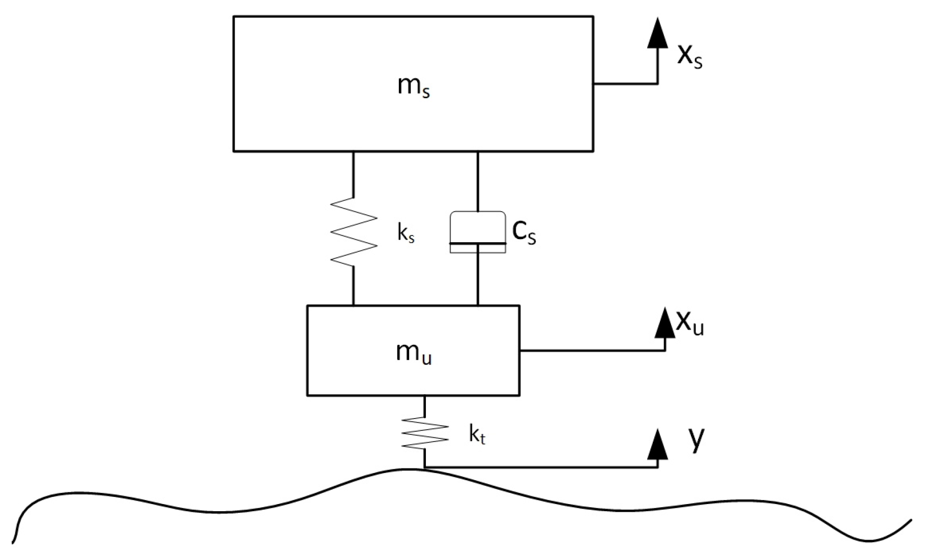
Lumped parameter models of a vehicle can differ in the number of degrees of freedom (DOFs), the planes where the movement of the vehicle is simulated (vertical, transverse, longitudinal), the inclusion of nonlinearities in the stiffness and damping elements and the consideration of control strategies in terms of semi-active and active suspension systems [10,11,12,13,14,15,16,17,18,19,20]. The simplest lumped parameter model of a suspension system is the Quarter Car (QC) model which consists of two masses (sprung and unsprung mass) interconnected with a stiffness and a damping element. Furthermore, a stiffness element is used to simulate the tire stiffness [11,21]. The QC model has two DOFs and simulates the movement of the vehicle in the vertical plane. According to Verros et al. [22] such a lumped parameter model subjected to excitation is commonly employed in the automotive industry mostly to predict the dynamic response identification, optimization and control of ground vehicles. The same model is also used in the automotive industry for the preliminary design of the suspension of a vehicle. The common use of this vehicle model is due to its simplicity and the fact that it provides qualitatively correct information, especially for ride and handling studies.

Similarly, the lumped parameter models of the driver (seated human body) are characterized by the number of DOFs which varies according to the total number of masses used to simulate the human body in a seated position [23,24] and correspond to its level of detail. Furthermore, these models differ in the way these masses are connected to each other (parallel or in series). Finally, they can contain linear or nonlinear stiffness and damping elements. It is important to note that since the human body is a complex structure, the parameters of the lumped parameter models are not consistent with the actual parameters of human anatomy and biodynamics [24]. One of the first lumped parameter models of the human body is a one DOF linear model developed by Coermann in 1962. In 1974, Muksian and Nash [25] developed a two DOFs nonlinear model to describe the dynamic response of the human body under different excitation frequencies. A two DOFs linear model was developed by Wei and Griffin in 1998 [26] to predict the seat transmissibility. A three DOFs linear model was also developed from Gao et al. [27] and later on from Kang [28]. Boileau and Rakheja [29] modeled the human body using a four DOFs lumped parameter model including nonlinearities in the stiffness and the damping elements parameters [30].

In the literature, the abovementioned models have been integrated into vehicle models, including the seat or not, in order to provide estimates of the vibrations induced in the human body while in a moving vehicle. The integrated Vehicle–Seat–Human (VSH) models are widely used for the optimization of the characteristics of the vehicle suspension considering road holding and ride comfort with a variety of objectives. The root-mean-square (RMS) value of the driver’s head acceleration is often included as an optimization objective for optimal suspension and/or seat design. In [30], head acceleration, its crest factor, the suspension deflection and the tire deflection were used, combined as one objective function in order to optimize the properties of a driver’s seat and the suspension of a vehicle using Genetic Algorithms. Later, Abbas [31,32], again using Genetic Algorithms, used an objective function combining head and seat acceleration as well as seat working space, in order to obtain the optimal design of a seat suspension. A similar objective function with the same optimization algorithm was also used [33,34] to optimize the parameters of a suspension system, also considering ride comfort. Furthermore, in [34] three objective functions were used and the Pareto front was created. Searching for an optimal design with a nonlinear passive suspension system [35] and for an optimal semi-active suspension [36,37], the values of the vibration dose of the head and the crest factor of the head were also used. Nagarkar [21,38] also considered the RMS head acceleration along with the amplitude ratio of the head RMS acceleration to seat RMS acceleration, the amplitude ratio of the upper torso RMS acceleration to seat RMS acceleration, the crest factor, the suspension space deflection and the dynamic tire deflection in order to optimize a passive suspension and later, present control strategies for an active suspension. In 2020, the head acceleration was used as a metrics for ride comfort in order to evaluate the performance of a magneto-rheological damper implemented for a seat suspension [3].

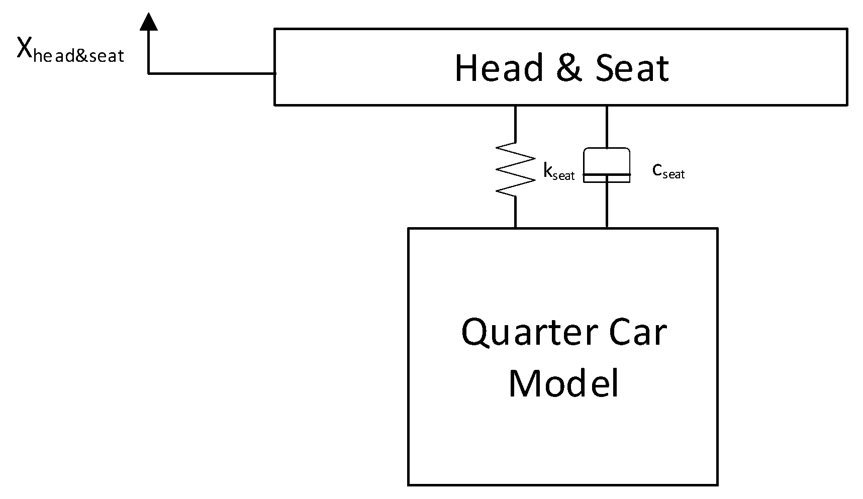
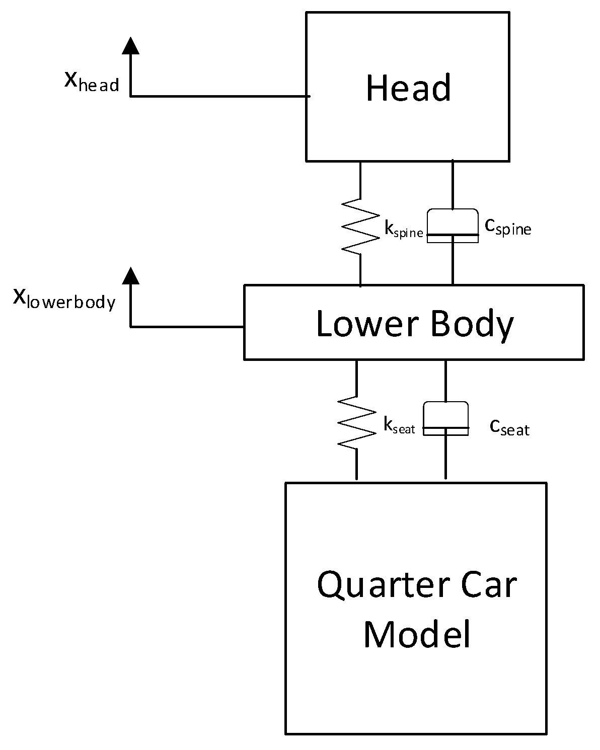
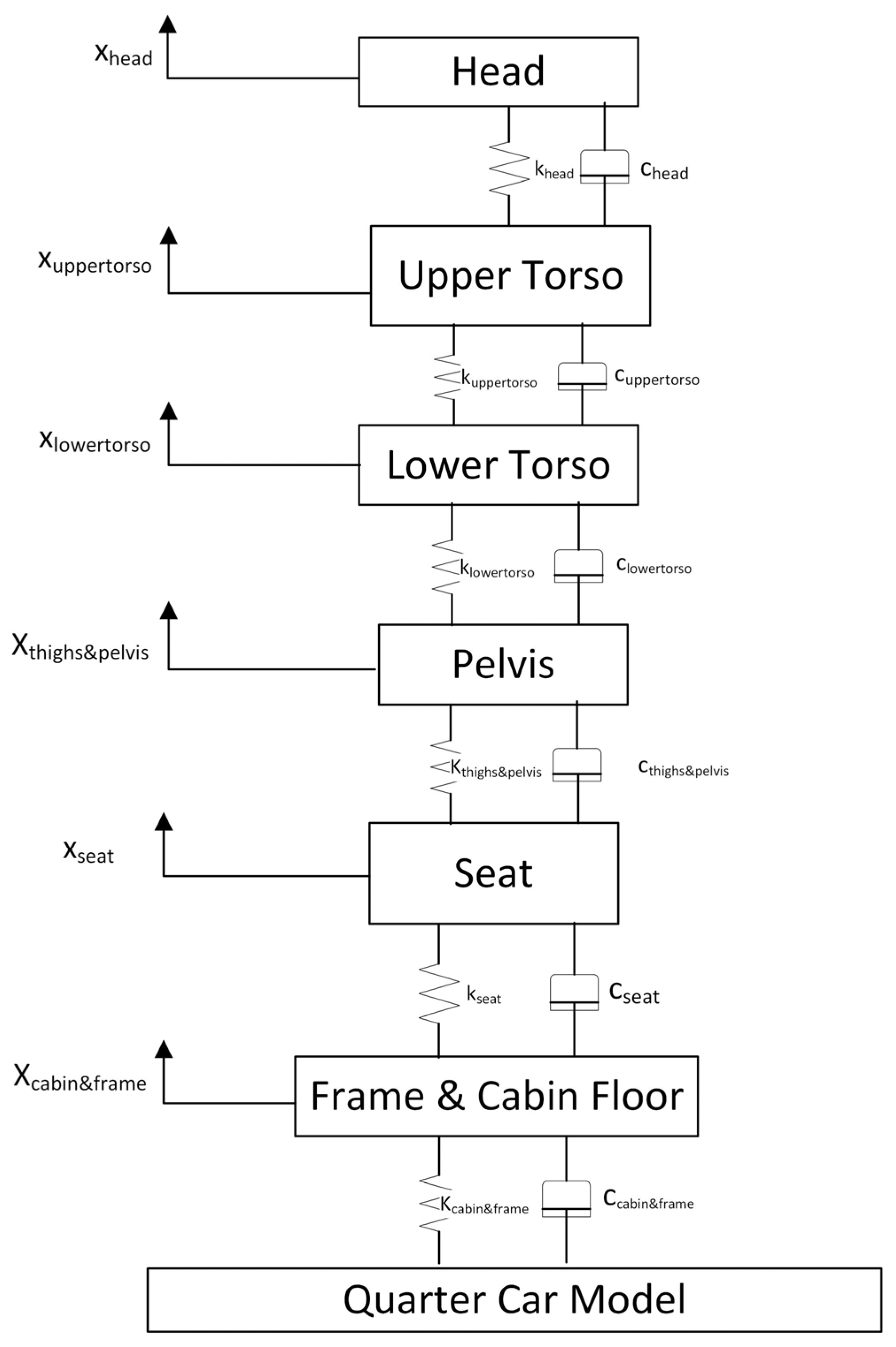
In the present paper, the performance of three VSH models, with three, four and eight DOFs based on the QC model was explored and compared in terms of efficiency with the QC model. All VSH models have already been used in the literature in ride comfort evaluation studies. The objective of this work is to indicate the minimum required level of detail of a lumped parameter model used to evaluate ride comfort in the vertical plane. The minimum required number of DOFs is important for both computational efficiency and simulation accuracy, since for each VSH model, the values of their lumped parameters should be set to simulate the vehicle, the seat and the human body characteristics as closely as possible.

Within this framework, two, three, four and eight DOFs models have been set up in the Matlab programming environment and they have been compared in terms of dynamic response and computational efficiency using excitations of different characteristics and different longitudinal velocities for the vehicle. This way the effect of the level of detail of the lumped parameter model can be also associated with the excitation and the longitudinal velocity. It should be noted that the values of the parameters (masses, stiffness coefficients and damping coefficients) of the VSH model were modified from those retrieved in the literature in order to simulate the same seat and human body, as closely as possible.

In Section 2 and Section 3 all lumped parameter models and excitations are described, respectively. In Section 4 the dynamic response of each model is presented for all excitations and three different longitudinal velocities of the vehicle. Then, in Section 5, the performance of the VSH models in terms of the head acceleration and the computational efficiency is monitored in the same excitations and the results are thoroughly discussed.

2. Lumped Parameter Models

In this section, firstly the QC model, used as a basis in all VSH models, is presented in terms of equations and parameter values. Then, the VSH models retrieved from the literature are described in detail.

2.1. QC Model

QC models are suitable for ride comfort evaluation since the longitudinal and transverse deflections of the suspension components due to the unevenness of the road profile can be considered negligible compared to the ones in the vertical direction. In the literature different values can be found for the lumped parameters of a QC model simulating different types of vehicles. Particularly, the value of the sprung mass ranges from 90 [39] to 476 kg [40] while the value of the unsprung mass ranges from 20 kg [3] to 80 kg [41]. Moreover, the values of the stiffness and the damping coefficients of the suspension lay in the ranges of 9000 $\frac{\mathrm{N}}{\mathrm{m}}$ [42] to 30,000 $\frac{\mathrm{N}}{\mathrm{m}}$ [43] and 980 $\frac{\mathrm{N}·\mathrm{s}}{\mathrm{m}}$ to 4300 $\frac{\mathrm{N}·\mathrm{s}}{\mathrm{m}}$ [44], respectively.

In this study, the QC model consisted of a sprung mass $m_s=270\mathrm{kg}$ connected to the unsprung mass, considered to have the value of 10% of the sprung mass, $m_u=27 \mathrm{kg}$. The unsprung mass was connected to the sprung mass via the suspension system that was simulated with a linear spring of stiffness $k_s=\mathrm{20,000} \frac{\mathrm{N}}{\mathrm{m}}$ [45] and a linear damper with a damping coefficient $c_s=2000 \frac{\mathrm{N}·\mathrm{s}}{\mathrm{m}}$ [3], which corresponds to 10% of the value of the stiffness coefficient. The tire stiffness was modeled as a vertical spring with a stiffness coefficient $k_t=\mathrm{160,000} \frac{\mathrm{N}}{\mathrm{m}}$ [7]. The tire damping coefficient was considered negligible and no nonlinearities were considered. This QC model simulated a typical, compact passenger’s car weighing 1188 $\mathrm{kg}$ and its schematic is presented in Figure 1.

The dynamic model of the system was a coupled linear differential equation set with two system variables of $x_s$ and $x_u$ for a given excitation $y$, as presented below (Equations (1) and (2)).

$$m_s·\ddot{x_s}=-k_s·(x_s-x_u)-c_s·\left(\dot{x_s}-\dot{x_u}\right)$$

(1)

$$m_u·\ddot{x_u}=k_s·\left(x_s-x_u\right)+c_s·\dot{(x_s}-\dot{x_u})-k_u·\left(x_u-y\right)$$

(2)

In

Table 1. Values of the first eigenfrequency of the sprung and the unsprung mass of the QC model.

Mass	1st Eigenfrequency
Sprung	1.29
Unsprung	12.99

the first eigenfrequency of the sprung and the unsprung mass is presented.

2.2. Three DOFs VSH Model

The three DOFs VSH model was presented in the literature by Kuznetsov et al. [46] and it was used for the optimization of a QC model subjected to a periodic road excitation. The proposed model consisted of three masses: the mass of the human body and the seat ($m_{head\&seat}=70 \mathrm{kg}$), the sprung mass (vehicle body) and the unsprung mass (vehicle wheel and other unsprung parts). The $m_{head\&seat}$ was connected to the QC model with a stiffness element ($k_{seat}=5600 \frac{\mathrm{N}}{\mathrm{m}}$) and a damping element ($c_{seat}=520 \frac{\mathrm{N}·\mathrm{s}}{\mathrm{m}}$). The schematic of the three DOFs VSH model is presented in Figure 2.

The dynamic model of this system was a set of three coupled linear differential equations with the three system variables of $x_{head\&seat}$, $x_s$ and $x_u$ for a given excitation $y$, as presented below (Equations (3)–(5)).

$$m_{head\&seat}·\ddot{x_{head\&seat}}=-k_{seat}·(x_{head\&seat}-x_{seat})-c_{seat}·\left(\dot{x_{head\&seat}}-\dot{x_{seat}}\right)$$

(3)

$$\begin{gathered} m_s·\ddot{x_s}=k_{seat}·\left(x_{head\&seat}-x_s\right)+c_{seat}·\dot{(x_{head\&seat}}-\dot{x_s})-k_s·(x_s-x_u)-c_s \\ ·\dot{(x_s}-\dot{x_u}) \end{gathered}$$

(4)

$$m_u·\ddot{x_u}=k_s·\left(x_s-x_u\right)+c_s·\left(\dot{x_s}-\dot{x_u}\right)-k_u·(x_u-y)$$

(5)

2.3. Four DOFs VSH Model

In Figure 3 the VSH model with four DOFs is presented.

This model was proposed by Mitra et al. in 2016 [34]. It consisted of four DOFs and it was also used in the optimization of the suspension of a passenger vehicle. The road profile used to evaluate the suspension behavior with respect to the ride comfort was a sinusoidal wave of height 0.1 m and a width of 1 m. In this model the human body was divided into two masses: the mass of the head ($m_{head}=20 \mathrm{kg}$) and the mass of the lower body ($m_{lowerbody}=45 \mathrm{kg}$). The head is interconnected to the lower body with a stiffness element ($k_{spine}=\mathrm{45,000} \frac{\mathrm{N}}{\mathrm{m}}$) and damping element ($c_{spine}=1360 \frac{\mathrm{N}·\mathrm{s}}{\mathrm{m}}$), simulating the human spine. Furthermore, the seat was considered as a spring ($k_{seat}=\mathrm{20,000} \frac{\mathrm{N}}{\mathrm{m}}$) and a damper ($c_{seat}=1650 \frac{\mathrm{N}·\mathrm{s}}{\mathrm{m}}$) connecting the lower body of the human to the vehicle.

The behavior of this dynamic system can be described with a set of four coupled linear differential equations (Equations (6)–(9)), as follows.

$$m_{head}·\ddot{x_{head}}=-k_{spine}·\left(x_{head}-x_{lowerbody}\right)-c_{spine}·\left(\dot{x_{head}}-\dot{x_{lowerbody}}\right)$$

(6)

$$\begin{gathered} m_{lowerbody}·\ddot{x_{lowerbody}} \\ =k_{spine}·\left(x_{head}-x_{lowerbody}\right)+c_{spine}·(\dot{x_{head}}-\dot{x_{lowerbody})}-k_{seat}·(x_{lowerbody}-x_s)-c_{seat} \\ ·\left(\dot{x_{lowerbody}}-\dot{x_s}\right) \end{gathered}$$

(7)

$$m_s·\ddot{x_s}=k_{seat}·\left(x_{lowerbody}-x_s\right)+c_{seat}·\left(\dot{x_{lowerbody}}-\dot{x_s}\right)-k_s·(x_s-x_u)-c_s·\dot{(x_s}-\dot{x_u})$$

(8)

$$m_u·\ddot{x_u}=k_s·\left(x_s-x_u\right)+c_s·\left(\dot{x_s}-\dot{x_u}\right)-k_u·\left(x_u-y\right)$$

(9)

The system variables are four, namely $x_{head}$, $x_{lowerbody}$, $x_s$ and $x_u$ for a given excitation $y$.

2.4. Eight DOFs VSH Model

The last model that was evaluated was adopted by Nagarkar et al. in 2016 [21] and it consisted of eight DOFs (Figure 4).

The human body was modeled using the four DOFs lumped parameter human model suggested by Boileau and Rakheja [19]. This models consisted of the head and neck mass ($m_{head}=5.31 \mathrm{kg}$), the chest and upper torso mass ($m_{uppertorso}=28.49 \mathrm{kg}$), the lower torso mass ($m_{lowertorso}=8.62 \mathrm{kg}$) and the thigh and pelvis mass ($m_{thighs\&pelvis}=12.78 \mathrm{kg}$). These masses were interconnected with stiffness and damping elements with values that are presented in

Table 2. Values of the stiffness and damping elements for the human body model.

Parameter	Units	Value
$k_{head}$	$\frac{\mathrm{N}}{\mathrm{m}}$	310,000
$k_{uppertorso}$		183,000
$k_{lowertorso}$		162,800
$k_{thighs\&pelvis}$		90,000
$c_{head}$	$\frac{\mathrm{N}·\mathrm{s}}{\mathrm{m}}$	400
$c_{uppertorso}$		4.750
$c_{lowertorso}$		4.585
$c_{thighs\&pelvis}$		2.064

.

The seat was modeled as two masses, one for the seat cushion ($m_{seat}=1 \mathrm{kg}$) and one for the cabin and frame ($m_{cabin\&frame}=15 \mathrm{kg}$). This models the frame of the seat and its mounting on the vehicle body. The two masses were connected to each other with a stiffness element ($k_{seat}=\mathrm{18,000} \frac{\mathrm{N}}{\mathrm{m}}$) and a damping element ($c_{seat}=200 \frac{\mathrm{N}·\mathrm{s}}{\mathrm{m}}$). Similarly, the cabin and frame mass were connected to the vehicle with a stiffness element ($k_{cabin\&frame}=\mathrm{31,000} \frac{\mathrm{N}}{\mathrm{m}}$) and a damping element ($c_{cabin\&frame}=830 \frac{\mathrm{N}·\mathrm{s}}{\mathrm{m}}$).

The behavior of this dynamic system can be described with a set of eight coupled linear differential equations (Equations (10)–(17)), as follows.

$$m_{head}·\ddot{x_{head}}=-k_{head}·\left(x_{head}-x_{uppertorso}\right)-c_{head}·\left(\dot{x_{head}}-\dot{x_{uppertorso}}\right)$$

(10)

$$\begin{gathered} m_{uppertorso}·\ddot{x_{uppertorso}} \\ =k_{head}·\left(x_{head}-x_{uppertorso}\right)+c_{head}·\left(\dot{x_{head}}-\dot{x_{uppertorso}}\right)-k_{uppertorso}·\left(x_{uppertorso} \\ -x_{lowertorso}\right)-c_{uppertorso}·\left(\dot{x_{uppertorso}}-\dot{x_{lowertorso}}\right) \end{gathered}$$

(11)

$$\begin{gathered} m_{lowetorso}·\ddot{x_{lowertorso}} \\ =k_{uppertorso}·\left(x_{uppertorso}-x_{lowrtorso}\right)+c_{uppertorso}·\left(\dot{x_{uppertorso}}-\dot{x_{lowertorso}}\right)-k_{lowertorso} \\ ·\left(x_{lowertorso}-x_{thighs\&pelvis}\right)-c_{lowertorso}·\left(\dot{x_{lowertorso}}-\dot{x_{thighs\&pelvis}}\right) \end{gathered}$$

(12)

$$\begin{gathered} m_{lhighs\&pelvis}·\ddot{x_{lhighs\&pelvis}} \\ =k_{lowertorso}·\left(x_{lowertorso}-x_{lhighs\&pelvis}\right)+c_{uppertorso}·\left(\dot{x_{lowertorso}}-\dot{x_{thighs\&pelvis}}\right)-k_{thighs\&pelvis} \\ ·\left(x_{thighs\&pelvis}-x_{seat}\right)-c_{thighs\&pelvis}·\left(\dot{x_{thighs\&pelvis}}-\dot{x_{seat}}\right) \end{gathered}$$

(13)

$$\begin{gathered} m_{seat}·\ddot{x_{seat}}=k_{thighs\&pelvis}·\left(x_{thighs\&pelvis}-x_{seat}\right)+c_{thighs\&pelvis}·\left(\dot{x_{thighs\&pelvis}}-\dot{x_{seat}}\right)-k_{seat}·\left(x_{seat} \\ -x_{cabin\&frame}\right)-c_{seat}·\left(\dot{x_{seat}}-\dot{x_{cabin\&frame}}\right) \end{gathered}$$

(14)

$$\begin{gathered} m_{cabin\&frame}·\ddot{x_{cabin\&frame}} \\ =k_{seat}·(x_{seat}-x_{cabin\&frame})+c_{seat}·\left(\dot{x_{seat}}-\dot{x_{cabin\&frame}}\right)-k_{cabin\&frame}·\left(x_{cabin\&frame}-x_s\right) \\ -c_{cabin\&frame}·\left(\dot{x_{cabin\&frame}}-\dot{x_s}\right) \end{gathered}$$

(15)

$$m_s·\ddot{x_s}=k_{cabin\&frame}·\left(x_{cabin\&frame}-x_s\right)+c_{cabin\&frame}·\left(\dot{x_{cabin\&frame}}-\dot{x_s}\right)-k_s·\left(x_s-x_u\right)-c_s·\left(\dot{x_s}-\dot{x_u}\right)$$

(16)

$$m_u·\ddot{x_u}=k_s·\left(x_s-x_u\right)+c_s·\left(\dot{x_s}-\dot{x_u}\right)-k_u·\left(x_u-y\right)$$

(17)

There are eight system variables for this VSH model: $x_{head}$, $x_{uppertorso}$, $x_{lowertorso}$, $x_{thighs\&pelvis}$, $x_{seat}$, $x_{cabin\&frame}$, $x_s$ and $x_u$ for a given excitation $y$.

2.5. Modified VSH Models

In order to evaluate the performance of the VSH models described above in terms of the dynamic behavior, the values of the lumped parameters were set in order to simulate the same vehicle and a seat and a human of the same mass. In all VSH models the QC model described in Section 2.1 was used as the vehicle model. Consequently, the mass of the human was considered equal to $m_{human}=90 \mathrm{kg}$ and the mass of the seat was considered equal to $m_{seat}=25 \mathrm{kg}$. Additionally, the hypothesis that 78% of the weight of the human body is supported by the seat in a seated position was assumed. This is an approximation based on the findings of Boileau et al. [47] who mention that 73.6% of the weight of a seated person is supported by the seat. Furthermore, the values of the stiffness and damping elements interconnecting the seat and the human body were kept the same.

In

Table 3. Values of the parameters of the seat and human model in the three DOFs VSH model.

Parameter	Units	Value
$m_{head\&seat}$	$\mathrm{kg}$	95
$k_{seat}$	$\frac{\mathrm{N}}{\mathrm{m}}$	15,000
$c_{seat}$	$\frac{\mathrm{N}·\mathrm{s}}{\mathrm{m}}$	500

the values of the three DOFs VSH model are presented.

In

Table 4. Values of the parameters of the seat and human model in the four DOFs VSH model.

Parameter	Units	Value
$m_{head}$	$\mathrm{kg}$	7
$m_{lowerbody}$		88
$k_{spine}$	$\frac{\mathrm{N}}{\mathrm{m}}$	200,000
$k_{seat}$		15,000
$c_{spine}$	$\frac{\mathrm{N}·\mathrm{s}}{\mathrm{m}}$	350
$c_{seat}$		500

the values of the four DOFs VSH model are presented.

In

Table 5. Values of the parameters of the seat and human model in the eight DOFs VSH model.

Parameter	Units	Value
$m_{head}$	$\mathrm{kg}$	7
$m_{uppertorso}$		21
$m_{lowertorso}$		10.5
$m_{thighs\&pelvis}$		31.5
$m_{seat}$		10
$m_{cabin\&frame}$		15
$k_{head}$	$\frac{\mathrm{N}}{\mathrm{m}}$	200,000
$k_{uppertorso}$		80,000
$k_{lowertorso}$		150,000
$k_{thighs\&pelvis}$		15,000
$k_{seat}$		1.500
$k_{cabin\&frame}$		700,000
$c_{head}$	$\frac{\mathrm{N}·\mathrm{s}}{\mathrm{m}}$	350
$c_{uppertorso}$		500
$c_{lowertorso}$		500
$c_{thighs\&pelvis}$		2.500
$c_{seat}$		500
$c_{cabin\&frame}$		70

the values of the eight DOFs VSH model are presented.

3. Excitations

One of the parameters influencing the performance of the QC model is the road input detail [45]. Consequently, three different types of excitations were induced in order to evaluate the performance of the VSH models: (a) single disturbance excitations, (b) a periodic one and (c) stochastic ones. Furthermore, for each excitation three different vehicle speeds were considered.

3.1. Single Disturbance Excitations

Two single disturbance excitations were induced, a bump and a pothole. The bump was modeled as a trapezoid with a height of 0.010 m and a length of 0.500 m, as it is presented in Figure 5.

The pothole is considered of the same length but its depth was considered equal to 0.040 m as it is presented in Figure 6.

The different crossing speeds of the vehicle considered for the single disturbance excitations were 5 $\frac{\mathrm{km}}{\mathrm{h}}$, 10 $\frac{\mathrm{km}}{\mathrm{h}}$ and 15 $\frac{\mathrm{km}}{\mathrm{h}}$.

3.2. Periodic Excitation

In Figure 7 the periodic disturbance is presented.

In this case the road profile was simulated as a sinusoidal excitation with an amplitude of 0.005 m and wavelength of the road profile changing with the speed of the vehicle which was considered equal to 30 $\frac{\mathrm{km}}{\mathrm{h}}$, 50 $\frac{\mathrm{km}}{\mathrm{h}}$ and 80 $\frac{\mathrm{km}}{\mathrm{h}}$.

3.3. Stochastic Excitations

Stochastic excitations involve random road profiles, generated based on the ISO 8086 [48], that classifies road profiles according to the quality of the road. According to this ISO, the road roughness classification can be performed using the power spectral density (PSD) values as shown

Table 6. The ISO classification of road roughness.

	$\mathbf{Degree}\mathbf{of}\mathbf{Roughness}\mathbf{in}{10}^{-6}{\mathit{m}}^3$$\mathit{\Phi }\left({\mathit{\Omega }}_0\right)$$\mathbf{Where}{\mathit{\Omega }}_0=1 \frac{\mathit{r}\mathit{a}\mathit{d}}{\mathit{m}}$
Road Class	Lower Limit	Geometric Mean	Upper Limit
A (very good)	-	16	32
B	32	64	128
C	128	256	512
D	512	1.024	2.048
E (very poor)	2.048	4.096	8.192

. Random road profiles can be approximated by a PSD using Equation (18):

$$\Phi \left(\Omega \right)=\Phi \left({\Omega }_0\right)·{\left(\frac{\Omega }{{\Omega }_0}\right)}^{-w}$$

(18)

where $\Omega =\frac{2·\pi }{L}$ denotes the angular spatial frequency in $\frac{\mathrm{rad}}{\mathrm{m}},$ $\Phi \left({\Omega }_0\right)$ denotes the value of the PSD at a reference wave number and $w$ is the waviness. For most road surfaces this can be considered equal to 2.

For this study, road profiles of Road Class A, C and E were depicted, in order to compare the performance of the different VSH models. In Figure 8, the classification of Road Classes can be verified as Class A being the one with the smoothest road profile, and Class E being the worst one.

For the stochastic excitations, the speed of the vehicle is considered as 30 $\frac{\mathrm{km}}{\mathrm{h}}$, 50 $\frac{\mathrm{km}}{\mathrm{h}}$ and 80 $\frac{\mathrm{km}}{\mathrm{h}}$.

4. Results

Initially, the dynamic response of the QC model, presented in Section 2.1, which is common in all VSH models, was monitored for all excitations, presented in Section 3, and all vehicle speeds. Then, the time history of the acceleration of the top DOF ($x_{head\&seat}$ for the three DOFs and $x_{head}$ for both the four and eight DOFs VSH models, presented in Section 2.2, Section 2.3 and Section 2.4 with the lumped parameter values presented in Section 2.5) was calculated for all excitations and vehicle speeds. The acceleration in all VSH models and the QC model as well was monitored with a sampling frequency of 200 Hz, since the frequency bands under consideration for the comfort and perception range from 0.5 Hz to 80 Hz [1].

4.1. Dynamic Response of the QC Model

In Figure 9 the calculated vertical displacement of the sprung mass versus the position of the vehicle on the longitudinal axis, for all vehicle speeds is presented for the bump, the pothole and the periodic excitation.

The same results are presented for road profiles of Classes A, C and E in Figure 10.

According to ISO2631-1 [1], the evaluation of vibrations shall include measurements of the weighted root-mean-square (RMS) acceleration. The RMS value of the acceleration for each DOF accordingly can be evaluated using Equation (19):

$$RMS\ddot{x_z}=\sqrt{\frac{1}{T}·{{\displaystyle \int }}_0^T\ddot{x_w{}^2}dt}$$

(19)

where $\ddot{x_w}$ is the acceleration as a function of time. Since only the vertical acceleration is calculated there is no need to take into account the $w_k$ weighting factor provisioned in ISO2631-1 [1].

In the case of the singular disturbance events, also peak acceleration has to be considered. For that reason, the fourth power vibration dose (VDV) method was used [1]. The definition of VDV in m/s^1.75 is provided in Equation (20).

$$VDV={\left[{{\displaystyle \int }}_0^T\ddot{x_w{}^4}dt\right]}^{\frac{1}{4}}$$

(20)

In

Table 7. The values of the peak accelerations of the sprung and the unsprung mass of the QC model for the single disturbance excitations.

Excitation		$5\frac{\mathbf{k}\mathbf{m}}{\mathbf{h}}$	$10\frac{\mathbf{k}\mathbf{m}}{\mathbf{h}}$	$15\frac{\mathbf{k}\mathbf{m}}{\mathbf{h}}$
	DOF	$\mathbf{Peak}\mathbf{Value}\mathbf{of}\mathbf{Vertical}\mathbf{Acceleration}\left(\frac{\mathbf{m}}{{\mathbf{s}}^2}\right)$
Bump	Sprung mass	1.24	2.36	2.81
	Unsprung mass	5.97	13.03	17.85
Pothole	Sprung mass	5.09	10.91	12.70
	Unsprung mass	23.71	53.06	71.95

the maximum value of the acceleration calculated for the sprung and unsprung mass are presented for both the single disturbance excitations.

In

Table 8. The VDV of the sprung mass of the QC model for the single disturbance excitations.

Excitation	$5\frac{\mathbf{k}\mathbf{m}}{\mathbf{h}}$	$10\frac{\mathbf{k}\mathbf{m}}{\mathbf{h}}$	$15\frac{\mathbf{k}\mathbf{m}}{\mathbf{h}}$
Bump	0.67	1.15	1.29
Pothole	2.74	4.62	5.18

the VDV of the sprung mass for the single excitation events is provided.

In

Table 9. The values of the RMS of acceleration for the sprung and the unsprung mass of the Quarter Car model for the periodic excitation.

Excitation		$30\frac{\mathbf{k}\mathbf{m}}{\mathbf{h}}$	$50\frac{\mathbf{k}\mathbf{m}}{\mathbf{h}}$	$80\frac{\mathbf{k}\mathbf{m}}{\mathbf{h}}$
	DOF	$\mathbf{RMS}\mathbf{Value}\mathbf{of}\mathbf{Vertical}\mathbf{Acceleration}\left(\frac{\mathbf{m}}{{\mathbf{s}}^2}\right)$
Periodic	Sprung mass	0.26	0.53	0.61
	Unsprung mass	0.17	0.46	1.09

the RMS values of the acceleration for the sprung and unsprung mass are presented for the periodic excitation.

In

Table 10. The values of the RMS of acceleration of the sprung and the unsprung mass of the Quarter Car model for the stochastic excitations.

Excitation		$30\frac{\mathbf{k}\mathbf{m}}{\mathbf{h}}$	$50\frac{\mathbf{k}\mathbf{m}}{\mathbf{h}}$	$80\frac{\mathbf{k}\mathbf{m}}{\mathbf{h}}$
	DOF	$\mathbf{RMS}\mathbf{Value}\mathbf{of}\mathbf{Vertical}\mathbf{Acceleration}\left(\frac{\mathbf{m}}{{\mathbf{s}}^2}\right)$
Class A	Sprung mass	0.03	0.04	0.05
	Unsprung mass	3.03	3.91	4.98
Class C	Sprung mass	0.13	0.18	0.22
	Unsprung mass	12.17	16.11	20.71
Class E	Sprung mass	0.53	0.69	0.90
	Unsprung mass	48.43	65.48	79.12

the RMS values of the acceleration of the sprung and unsprung mass are presented for the stochastic disturbance excitations.

4.2. Dynamic Response of the Top DOF in the VSH Models

In order to evaluate the performance of the VSH models, their dynamic response was calculated for all excitations and vehicle speeds. The criterion for the evaluation of their performance for the single disturbance excitations is the maximum, VDV and RMS value of the vertical acceleration of the top DOF of every VSH model.

In Figure 11 the peak, the VDV and the RMS value of the acceleration on the top DOF is presented for both singular disturbance events and all vehicle speeds.

For the periodic and the stochastic ones, only the RMS value of the acceleration was used as a criterion for the performance evaluation of the VSH models. The calculated RMS value of acceleration of the top DOF is presented in Figure 12 for the periodic excitation.

Finally, the same results are presented for road profiles of Class A, C and E in Figure 13.

In Figure 11, Figure 12 and Figure 13 the horizontal axis is the number of DOFs of the VSH model, hence each dot represents a different VSH model, starting from the QC model with 2 DOFs. Furthermore, the maximum value of the vertical axis is set to be the same for all excitations.

As mentioned above, the VSH models are often used for the optimization either of the vehicle suspension characteristics or the seat structure, mounting and suspension requesting a high number of iterations. In

Table 11. The CPU time for all the VSH models in Class A, C and E road profiles.

	CPU Time (s)
VSH Model	Class A	Class C	Class E
3 DOFs	2.33	2.35	2.45
4 DOFs	2.38	2.41	2.51
8 DOFs	2.53	2.62	2.63

the CPU time per evaluation for each model is presented for the stochastic excitations and the minimum speed of the vehicle.

5. Discussion

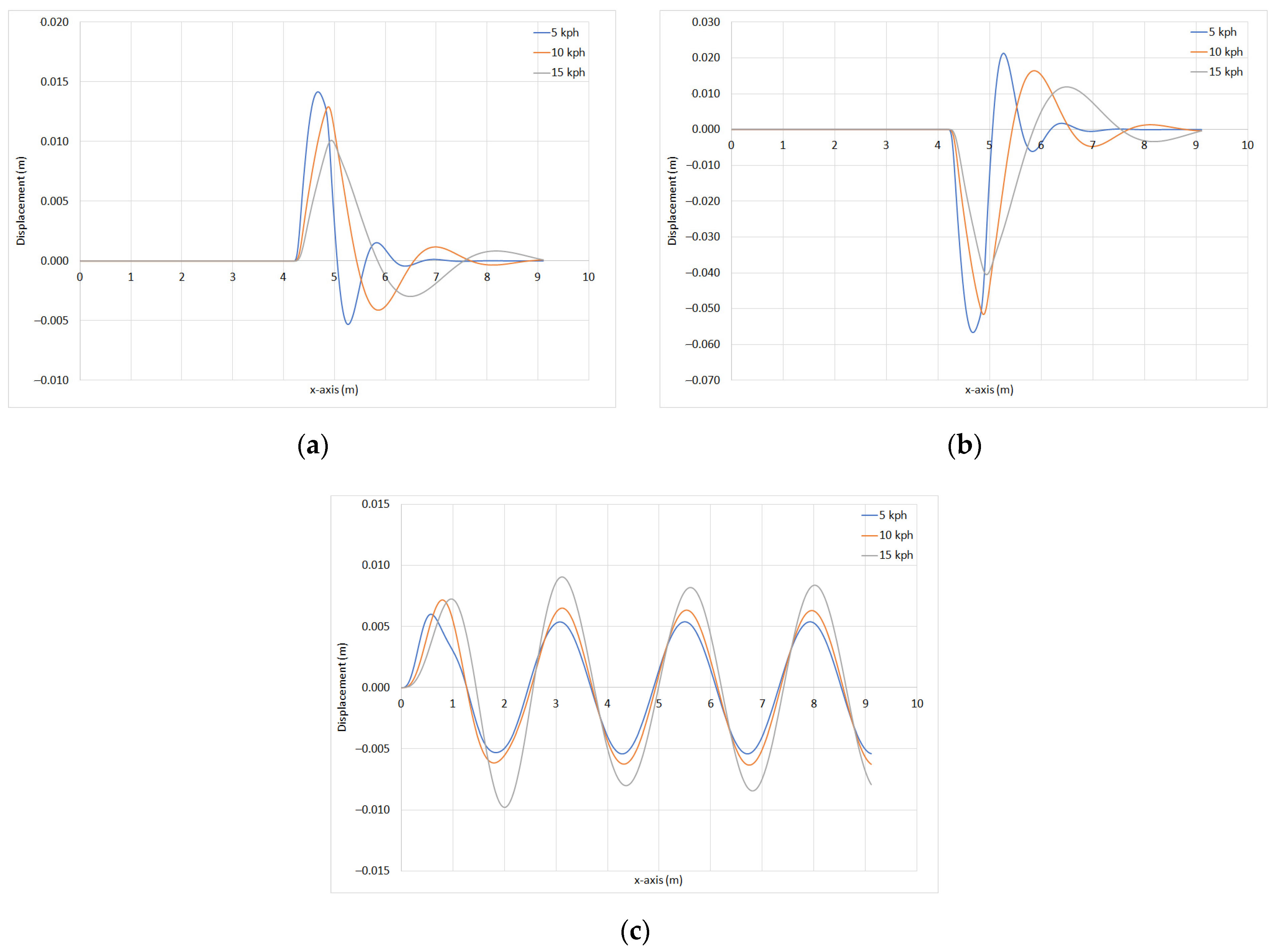
Firstly, the dynamic response of the QC model was explored, providing an insight into the vehicle model which is the base of all the presented VSH models in Section 2. In Figure 9 the vertical displacement versus the longitudinal location of the vehicle is presented showing that for the single disturbance events, as the speed of the vehicle increases the peak displacement decreases, while for the periodic excitation an increase in the speed of the vehicle causes an increase, also, in the maximum value of the vertical displacement of the sprung mass. 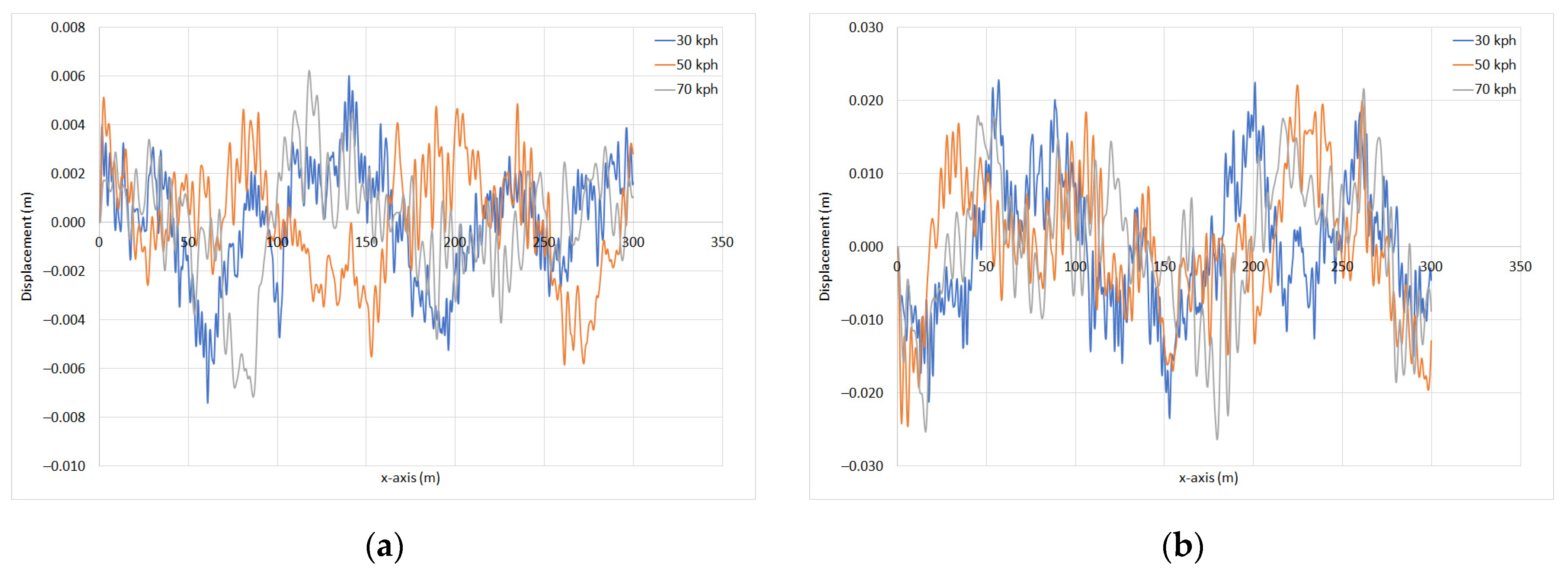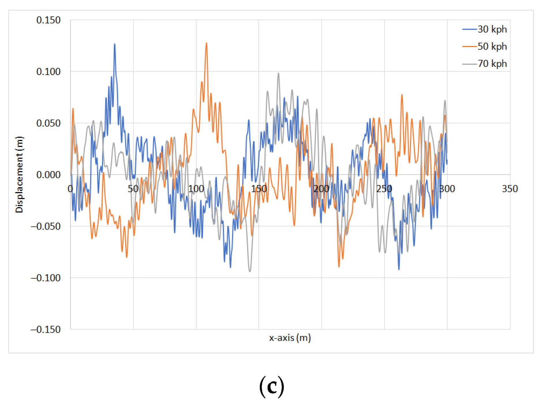In Figure 10, presenting the dynamic response of the QC model in stochastic excitations, there is no association of the maximum displacement with the vehicle speed but there is a straight association of the grade of the road profile with the maximum displacement. As it was expected, the maximum value of the vertical displacement was met for the road profiles of Grade E. Although ride comfort is directly correlated to acceleration, the displacement response of the QC model was presented in order to provide an overview of the response of the system.

In Table 7, Table 8, Table 9 and Table 10, where the peak (Table 7), the VDV (Table 8) and RMS (Table 9 and Table 10) values of the acceleration are provided for all excitations for the QC model, it is obvious that the sprung mass has lower values of vertical acceleration than the unsprung mass, as it was expected. Furthermore, in Table 7 and Table 8 it is shown that the provided pothole excitation consists of a rougher excitation than the bump. Moreover, the increase in the vehicle longitudinal velocity leads to an increase in the peak, the VDV and the RMS values of the vertical acceleration, depending on the type of excitation.

Given the dynamic response of the QC model, the dynamic response of the different VSH models is explored. In Figure 11, concerning single disturbance excitations, it is obvious that the peak, VDV and RMS values of the acceleration have the same behavior. Particularly, the QC model has the highest value of vertical acceleration of the top DOF, while the VSH model with eight DOFs has the lowest one. Furthermore, the VSH with three DOFs has almost the same value as the VSH model with four DOFs. In Figure 14 the difference in the VDV of the top DOF for the VSH models with respect to the VDV of the sprung mass DOF of the QC model is presented for the single disturbance events. For the three DOFs model the difference ranges from 18–51% depending on the excitation and the longitudinal velocity of the vehicle (blue corresponds to 5 km/h, orange to 10 km/h and grey to 15 km/h). For the four DOFs model the difference ranges from 35–69% and for the eight DOFs it ranges from 49–74%.

In Figure 14, as expected from the percentage (%) of difference, it is also obvious that in the case of the single disturbance excitations the relative behavior of all the models is the same regardless of the excitation. All the VSH models provide a lower VDV for their top DOF. The lowest VDV is provided by the top DOF of the VSH model with eight DOFs.

In Figure 12, concerning the periodic excitation it is observed that the VSH models with three and four DOFs have similar results, while the QC model has the lowest value of the RMS vertical acceleration followed by the VSH model with eight DOFs.

The same observation can also be made in Figure 15 where the difference between the RMS values of the vertical acceleration of the VSH models with respect to the QC model are presented, also taking into consideration the longitudinal velocity.

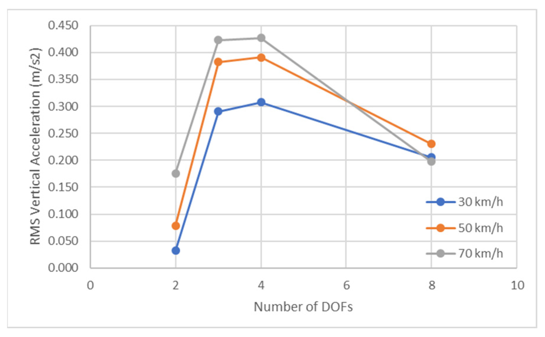
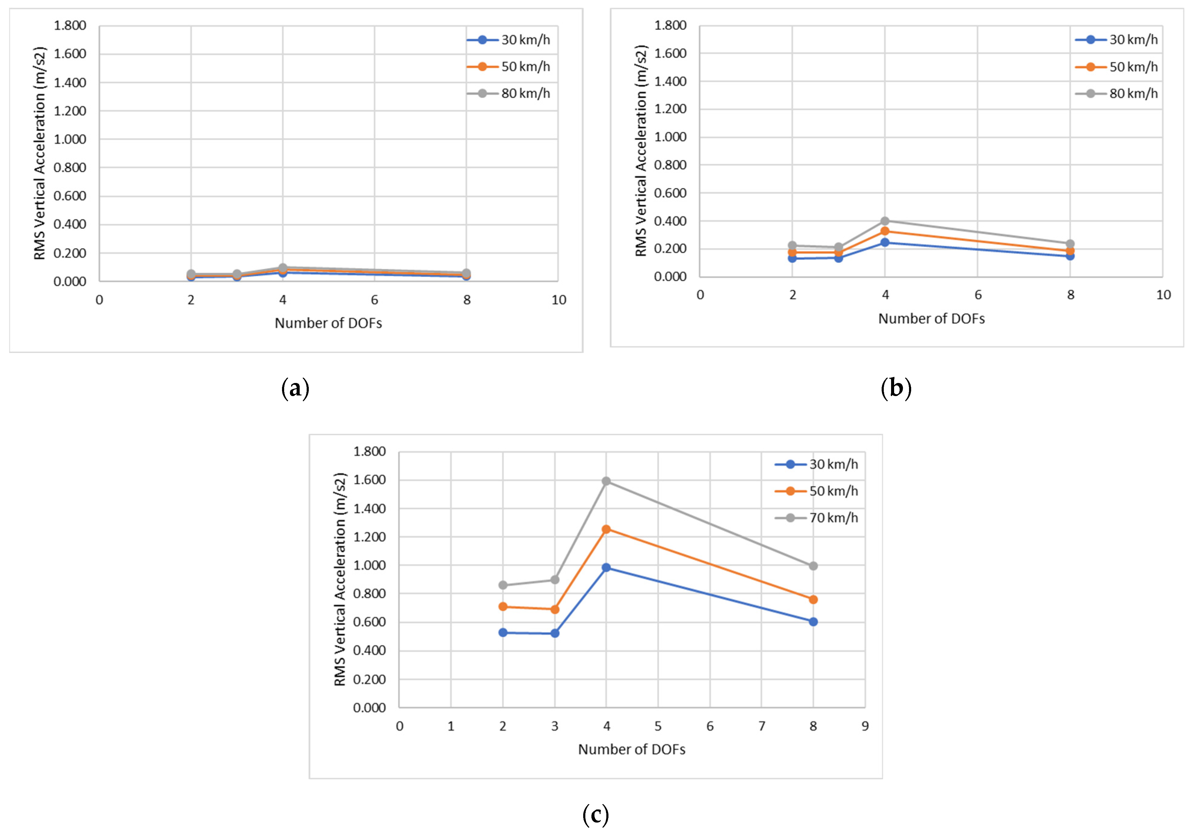
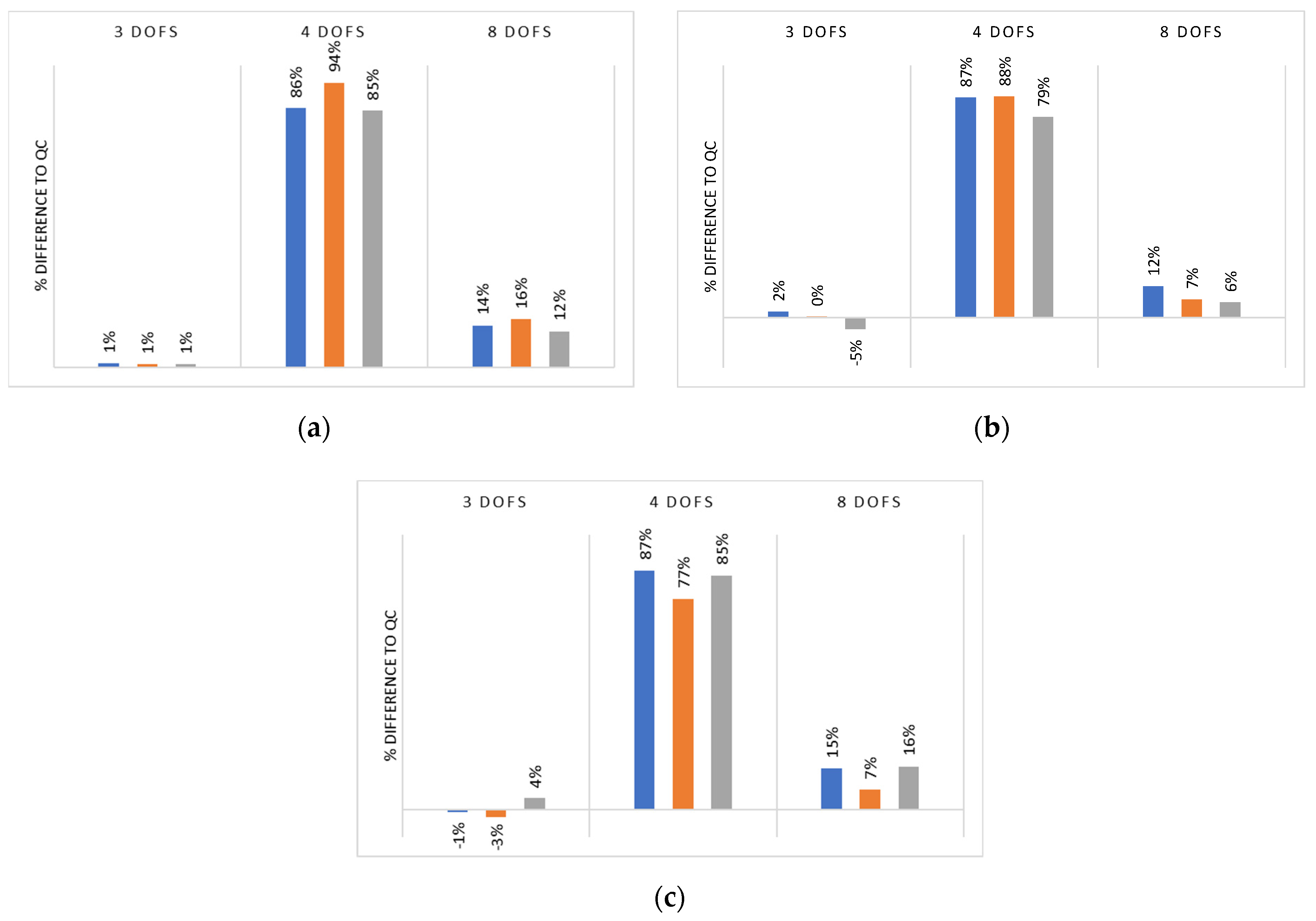
A similar behavior, concerning the VSH models can be observed also in Figure 13, presenting the RMS value of the vertical acceleration for the stochastic excitations. In more detail, the VSH model with four DOFs has the highest RMS value of vertical acceleration, the VSH model with three DOFs has the lowest one and the model with eight DOFs is close to that. On the other hand, in the case of the stochastic excitations the QC model has the lowest values of the RMS for the vertical acceleration. In Figure 16 the abovementioned percentage is provided for the road profiles of Class A, C and E.

In the case of the stochastic excitations, the VSH model with the four DOFs has an RMS value of an acceleration 70% higher than that of the QC model, while the VSH model with three DOFs provides a lower RMS value of vertical acceleration compared to the QC model that has a value less than 5%. The VSH model with eight DOFs provides RMS values of an acceleration that is 6–16% larger than that of the QC model. It is worth mentioning that in the case of the stochastic excitations, the longitudinal velocity of the vehicle does not affect the RMS value of the vertical acceleration of the top DOF of the VSH model in the same way as it does in the singular or the periodic excitations.

As far as the computational efficiency of the VSH models, in Table 11 it can be observed that an increase in the DOFs of the VSH model by 1 causes an increase in the CPU time from 2.1 to 2.6%, respectively, for the road profile while increasing the number of DOFs by 5 increases the CPU time from 7.4 to 11.5%.

The findings of this work can be considered consistent with the findings of [49] who compared a two, three and four DOFs model to experimental data, and they concluded that the two DOFs model provided results closest to the experimental ones.

6. Conclusions

The objective of this paper was to compare the performance of different existing VSH models used for the evaluation and the optimization of the ride comfort of vehicles in terms of the reliability and computational efficiency, in order to determine the minimum required number of DOFs for a VSH model. It is important to note that despite the number of DOFs required for the VSH model, the values of the used lumped parameters should be set in a way to simulate the vehicle, seat and human body characteristics as closely as possible. Thus, three lumped parameter VSH models with a different number of DOFs and a linear connection between the masses, based on a QC vehicle model and simulating the same vehicle, seat and human were set up in a Matlab programming environment. Their dynamic response to three types of excitations with different characteristics and different longitudinal velocities was calculated in terms of the acceleration, velocity and displacement.

The dynamic response was proven to be dependent on the number of DOFs of the VSH models, providing different peak, VDV and RMS values of the vertical acceleration. Moreover, the type of excitation affected the dynamic response of the VSH model with respect to that of the QC model. In particular, in the case of single disturbances, the VSH model with eight DOFs resulted in the lowest peak, VDV and RMS values of the acceleration for the top DOF. For the three DOFs model, the difference between its VDV and the VDV of the QC model ranged from 18–51% depending on the excitation and the longitudinal velocity of the vehicle. For the four DOFs model the difference ranged from 35–69% and for the eight DOFs it ranged from 49–74%. On the contrary, for the periodic excitation it was noticed that the VSH models with three and four DOFs provided close RMS values of the vertical acceleration for the top DOF, two to eight times larger than that of the QC model, while the eight DOFs model provided values up to five times larger than those of the QC model. Finally, in the case of the stochastic excitations the RMS values of both the VSH model with three and eight DOFs were close to those of the RMS values of the sprung mass of the QC model (−3 to 16%). The model with the four DOFs provided RMS values of the vertical acceleration that were 77–94% larger than those of the QC model.

As far as the computational efficiency of the VSH models is concerned, it was shown that the greater difference in the CPU time for one evaluation of the VSH models was less than 12%.

Taking into account the aforementioned observations, it becomes apparent that the selection of the proper VSH model based on a QC model depends solely on the requirements of the ride comfort study. Considering that the QC model, which is the base of all the investigated VSH models, simulates the vertical dynamic response of a vehicle in a qualitative manner, it is evident that there is no gain in considering a detailed Seat–Human system in a vertical VSH model when only the vehicle suspension is under investigation. Hence, in the case of the optimization of ride comfort, the minimum number of required DOFs should be defined with respect to the design variables and the objectives of the optimization procedure. Specifically, if the modeling objective is to optimize the ride comfort, altering the suspension characteristics the QC model (two DOFs) is sufficient while if the seat characteristics are going to be optimized, a VSH model consisting of three DOFs should be preferred as it is sufficient and computationally efficient. Finally, a VSH model with four DOFs (unsprung, sprung, seat, seated human body) should be used when the seat transmissibility is considered during the optimization procedure either as an objective or as a constraint.

References

1. Vibration, M. Shock—evaluation of human exposure to whole-body vibration—Part 1: General requirements. Int. Organ. Stand. ISO 1997, 2631-1. [Google Scholar]
2. Golubović-Bugarski, V.; Petković, S.; Đurić, Ž; Jotić, G. Vibration Comfort Of The Vehicle Expressed By Seat Effective Amplitude Transmissibility. Veh. Vozila I 2019, 1. [Google Scholar] [CrossRef]
3. Jain, S.; Saboo, S.; Pruncu, C.I.; Unune, D.R. Performance investigation of integrated model of quarter car semi-active seat suspension with human model. Appl. Sci. 2020, 10, 3185. [Google Scholar] [CrossRef]
4. Popp, K.; Schiehlen, W. Ground Vehicle Dynamics; Springer: Berlin/Heidelberg, Germany, 2010. [Google Scholar]
5. International Organization for Standardization. ISO 2631–5: Mechanical Vibration and Shock–Evaluation of Human Exposure to Whole-Body Vibration–Part V: Method for Evaluation of Vibration Containing Multiple Shocks; ISO: Geneva, Switzerland, 2018; Volume 2631-5. [Google Scholar]
6. Hamza, A.; Ben Yahia, N. Heavy trucks with intelligent control of active suspension based on artificial neural networks. Proc. Inst. Mech. Eng. Part I J. Syst. Control. Eng. 2021, 235, 952–969. [Google Scholar] [CrossRef]
7. Thomas, D.G. Fundamentals of Vehicle Dynamics; Society of Otomotif Engineers Inc.: Warrendale, PA, USA, 1994. [Google Scholar]
8. Koch, G. Adaptive Control of Mechatronic Vehicle Suspension Systems. Doctoral Dissertation, Technische Universität München, München, Germany, 2011. [Google Scholar]
9. Lugner, P. (Ed.) Vehicle Dynamics of Modern Passenger Cars; Springer: Cham, Switzerland, 2019. [Google Scholar]
10. Jazar, R.N. Vehicle Dynamics; Springer: New York, NY, USA, 2017; Volume 1. [Google Scholar]
11. Jazar, R.N. Advanced Vehicle Dynamics; Springer International Publishing: Cham, Switzerland, 2019. [Google Scholar]
12. Theunissen, J.; Tota, A.; Gruber, P.; Dhaens, M.; Sorniotti, A. Preview-based techniques for vehicle suspension control: A state-of-the-art review. Annu. Rev. Control. 2021, 51, 206–235. [Google Scholar] [CrossRef]
13. Ebrahimi-Nejad, S.; Kheybari, M.; Borujerd, S.V.N. Multi-objective optimization of a sports car suspension system using simplified quarter-car models. Mech. Ind. 2020, 21, 412. [Google Scholar] [CrossRef]
14. Sharma, S.; Chouksey, M.; Pare, V.; Jain, P. Modal and frequency response characteristics of vehicle suspension system using full car model. In IOP Conference Series: Materials Science and Engineering; IOP Publishing: Bristol, UK, 2020; Volume 810, p. 012056. [Google Scholar]
15. Wang, G.; Chen, C.; Yu, S. Optimization and static output-feedback control for half-car active suspensions with constrained information. J. Sound Vib. 2016, 378, 1–13. [Google Scholar] [CrossRef]
16. Hassanzadeh, I.; Alizadeh, G.; Shirjoposht, N.P.; Hashemzadeh, F. A new optimal nonlinear approach to half car active suspension control. Int. J. Eng. Technol. 2010, 2, 78. [Google Scholar] [CrossRef]
17. Ge, X.; Ahmad, I.; Han, Q.L.; Wang, J.; Zhang, X.M. Dynamic event-triggered scheduling and control for vehicle active suspension over controller area network. Mech. Syst. Signal Process. 2021, 152, 107481. [Google Scholar] [CrossRef]
18. Yoon, D.S.; Kim, G.W.; Choi, S.B. Response time of magnetorheological dampers to current inputs in a semi-active suspension system: Modeling, control and sensitivity analysis. Mech. Syst. Signal Process. 2021, 146, 106999. [Google Scholar] [CrossRef]
19. Hamza, A.; Ben Yahia, N. Intelligent neural network control for active heavy truck suspension. In Advances in Mechanical Engineering and Mechanics: Selected Papers from the 4th Tunisian Congress on Mechanics, CoTuMe 2018, Hammamet, Tunisia, 13–15 October 2018; Springer International Publishing: Cham, Switzerland, 2019; pp. 16–23. [Google Scholar]
20. Hamza, A.; Ben Yahia, N. Deep Learning Based Intelligent Active Suspension Control for Heavy Trucks (DMPSO). In Advances in Mechanical Engineering and Mechanics II: Selected Papers from the 5th Tunisian Congress on Mechanics, CoTuMe 2021, 22–24 March 2021; Springer International Publishing: Cham, Switzerland, 2022; pp. 347–354. [Google Scholar]
21. Nagarkar, M.P.; Patil, G.J.V.; Patil, R.N.Z. Optimization of nonlinear quarter car suspension–seat–driver model. J. Adv. Res. 2016, 7, 991–1007. [Google Scholar] [CrossRef] [Green Version]
22. Verros, G.; Natsiavas, S.; Papadimitriou, C. Design optimization of quarter-car models with passive and semi-active suspensions under random road excitation. J. Vib. Control. 2005, 11, 581–606. [Google Scholar] [CrossRef]
23. Ghasemi-Goneyrania, S.; Ali, M. Evaluation of Optimized Lumped-Parameter Models of Seated Human Body Exposed to Vertical Vibration. In Proceedings of the 10th ISAV2020, Tehran, Iran, 17–18 February 2021. [Google Scholar]
24. Bai, X.-X.; Xu, S.-X.; Cheng, W.; Qian, L.-J. On 4-degree-of-freedom biodynamic models of seated occupants: Lumped-parameter modeling. J. Sound Vib. 2017, 402, 122–141. [Google Scholar] [CrossRef]
25. Muksian, R.; Nash, C.D. A model for the response of seated humans to sinusoidal displacements of the seat. J. Biomech. 1974, 7, 209–215. [Google Scholar] [CrossRef]
26. Wei, L.; Griffin, J. The prediction of seat transmissibility from measures of seat impedance. J. Sound Vib. 1998, 214, 121–137. [Google Scholar] [CrossRef]
27. Gao, J.; Hou, Z.; He, L.; Xia, Q. Vertical vibration characteristics of seated human bodies and a biodynamic model with two degrees of freedom. Sci. China Technol. Sci. 2011, 54, 2776–2784. [Google Scholar] [CrossRef]
28. Kang, J. Human body vibration analysis under consideration of seat dynamic characteristics. J. Korea Acad. Coop. Soc. 2012, 13, 5689–5695. [Google Scholar]
29. Boileau, P.; Wu, X.; Rakheja, S. Definition of a range of idealized values to characterize seated body biodynamic response under vertical vibration. J. Sound Vib. 1998, 215, 841–862. [Google Scholar] [CrossRef]
30. Gündoğdu, Ö. Optimal seat and suspension design for a quarter car with driver model using genetic algorithms. Int. J. Ind. Ergon. 2007, 37, 327–332. [Google Scholar] [CrossRef]
31. Abbas, W.; Abouelatta, O.B.; El-Azab, M.S.; Megahed, A.A. Application of genetic algorithms to the optimal design of vehicle’s driver-seat suspension model. In Proceedings of the WCE 2010, London, UK, 30 June 30–2 July 2010. [Google Scholar]
32. Abbas, W.; Emam, A.; Badran, S.; Shebl, M.; Abouelatta, O. Optimal Seat and Suspension Design for a Half-Car with Driver Model Using Genetic Algorithm. Intell. Control. Autom. 2013, 4, 199–205. [Google Scholar] [CrossRef]
33. Salah, A.; Wael, A.; Ossama, B. Abouelatta. Design of optimal linear suspension for quarter car with human model using genetic algorithms. Res. Bull. Jordan 2010, 11, 42–51. [Google Scholar]
34. Mitra, A.C.; Desai, G.J.; Patwardhan, S.R.; Shirke, P.H.; Kurne, W.M.; Banerjee, N. Optimization of Passive Vehicle Suspension System by Genetic Algorithm. Procedia Eng. 2016, 144, 1158–1166. [Google Scholar] [CrossRef]
35. Koulocheris, D.; Papaioannou, G.; Chrysos, E. A comparison of optimal semi-active suspension systems regarding vehicle ride comfort. In IOP Conference Series: Materials Science and Engineering; IOP Publishing: Bristol, UK, 2017; Volume 252, p. 012022. [Google Scholar]
36. Koulocheris, D.; Papaioannou, G.; Christodoulou, D. Optimal design solution among pareto alternatives for vehicle nonlinear suspension system. In Proceedings of the 26th International Automotive Conference “Science and Motor Vehicles” (26th JUMV), Belgrade, Serbia, 19–20 April 2017. [Google Scholar]
37. Papaioannou, G.; Koulocheris, D. An approach for minimizing the number of objective functions in the optimization of vehicle suspension systems. J. Sound Vib. 2018, 435, 149–169. [Google Scholar] [CrossRef]
38. Nagarkar, M.P.; Bhalerao, Y.J.; Patil, G.V.; Patil, R.Z. Multi-objective optimization of nonlinear quarter car suspension system–PID and LQR control. Procedia Manuf. 2018, 20, 420–427. [Google Scholar] [CrossRef]
39. Koch, G.; Pellegrini, E.; Spirk, S.; Lohmann, B. Design and modeling of a quarter-vehicle test rig for active suspension control. In Lehrstuhl für Regelungstechnik; Technische Universität München: München, Germany, 2010. [Google Scholar]
40. Barethiye, V.M.; Pohit, G.; Mitra, A. Analysis of a quarter car suspension system based on nonlinear shock absorber damping models. Int. J. Automot. Mech. Eng. 2017, 14, 4401–4418. [Google Scholar] [CrossRef]
41. Pathare, Y.S.; Nimbalkar, S.R. Design and development of quarter car suspension test rig model and it’s simulation. Int. J. Innov. Res. Dev. 2014, 3, 157–170. [Google Scholar]
42. Bruqi, M.; Likaj, R.; Shala, A. Simulation of Vertical Quarter Car Model With One and Two DOFs. Mach. Technol. Mater. 2017, 11, 261–263. [Google Scholar]
43. Thite, A.N. Development of a refined quarter car model for the analysis of discomfort due to vibration. Adv. Acoust. Vib. 2012, 2012, 863061. [Google Scholar] [CrossRef]
44. Soong, M.F.; Ramli, R.; Saifizul, A. Between simplicity and accuracy: Effect of adding modeling details on quarter vehicle model accuracy. PLoS ONE 2017, 12, e0179485. [Google Scholar] [CrossRef]
45. Chen, X.; Song, H.; Zhao, S.; Xu, L. Ride comfort investigation of semi-active seat suspension integrated with quarter car model. Mech. Ind. 2022, 23, 18. [Google Scholar] [CrossRef]
46. Kuznetsov, A.; Mammadov, M.; Sultan, I.; Hajilarov, E. Optimization of a quarter-car suspension model coupled with the driver biomechanical effects. J. Sound Vib. 2011, 330, 2937–2946. [Google Scholar] [CrossRef]
47. Boileau, P.É.; Rakheja, S. Whole-body vertical biodynamic response characteristics of the seated vehicle driver: Measurement and model development. Int. J. Ind. Ergon. 1998, 22, 449–472. [Google Scholar] [CrossRef]
48. Technical Committee ISO/TC. Mechanical Vibration-Road Surface Profiles-Reporting of Measured Data; International Organization for Standardization: Geneva, Switzerland, 1995; Volume 8608. [Google Scholar]
49. Behari, N.; Noga, M. Vibration transmissibility behaviour of simple biodynamic models used in vehicle seat design. Czas. Tech. 2016, 2016, 3–12. [Google Scholar]
Figure 1. The QC Model.
Vehicles 05 00010 g001
Figure 2. The three DOFs VSH model.
Vehicles 05 00010 g002
Figure 3. The four DOFs VSH model.
Vehicles 05 00010 g003
Figure 4. The eight DOFs VSH model.
Vehicles 05 00010 g004
Figure 5. The bump excitation.
Vehicles 05 00010 g005
Figure 6. The pothole excitation.
Vehicles 05 00010 g006
Figure 7. The periodic disturbance.
Vehicles 05 00010 g007
Figure 8. The road profile of (a) Class A, (b) Class C and (c) Class E.
Vehicles 05 00010 g008
Figure 9. The vertical displacement of the sprung mass versus the position of the vehicle on the x-axis for the (a) bump, (b) pothole and (c) periodic excitation.
Vehicles 05 00010 g009
Figure 10. The vertical displacement of the sprung mass versus the position of the vehicle on the x-axis for road profiles of (a) Class A, (b) Class C and (c) Class E.
Vehicles 05 00010 g010aVehicles 05 00010 g010b
Figure 11. The peak, VDV and RMS values of the acceleration of the top DOF for the (a) bump and the (b) pothole excitation.
Vehicles 05 00010 g011aVehicles 05 00010 g011b
Figure 12. The RMS value of the acceleration of the top DOF for the periodic disturbance.
Vehicles 05 00010 g012
Figure 13. The RMS value of the acceleration of the top DOF for the road profile of Class (a) A, (b) C and (c) E.
Vehicles 05 00010 g013
Figure 14. The percent difference in the VDV of the top DOF for every model to the peak value of the acceleration of the top DOF of the QC model for the (a) bump and the (b) pothole excitation (blue = 5 km/h, orange = 10 km/h and grey = 15 km/h).
Vehicles 05 00010 g014
Figure 15. The percent difference in the RMS values of the acceleration of the top DOF of all models to the RMS values of the acceleration of the top DOF of the QC model for the periodic disturbance (blue = 5 km/h, orange = 10 km/h and grey = 15 km/h).
Vehicles 05 00010 g015
Figure 16. The percent difference of the RMS values of the acceleration of the top DOF of all models to the RMS values of the acceleration of the top DOF of the QC model for road profiles of (a) Class A, (b) Class C and (c) Class E (blue = 5 km/h, orange = 10 km/h and grey = 15 km/h).
Vehicles 05 00010 g016