Article

Estimation of Oral Exposure of Dairy Cows to the Mycotoxin Deoxynivalenol (DON) through Toxin Residues in Blood and Other Physiological Matrices with a Special Focus on Sampling Size for Future Predictions

1
Institute of Animal Nutrition, Friedrich-Loeffler-Institut (FLI), Federal Research Institute for Animal Health, Bundesallee 37, 38116 Braunschweig, Germany
2
Biometrics and Informatics in Agriculture Group, Institute of Agricultural and Nutritional Sciences, Martin-Luther-University Halle-Wittenberg, Karl-Freiherr-von-Fritsch-Str. 4, 06120 Halle, Germany
3
Department for Ruminants and Swine, Faculty of Veterinary Medicine, University of Leipzig, An den Tierkliniken 11, 04103 Leipzig, Germany
*
Author to whom correspondence should be addressed.
Dairy 2023, 4(2), 360-391; https://doi.org/10.3390/dairy4020024
Submission received: 10 April 2023 / Revised: 21 May 2023 / Accepted: 29 May 2023 / Published: 31 May 2023
(This article belongs to the Section Dairy Animal Health)

Abstract

:
Evaluation of dairy cow exposure to DON can generally be managed through analyses of feed or physiological specimens for DON residues. The latter enables a diagnosis not only on an individual basis but also on a herd basis. For this purpose, on the basis of published data, linear regression equations were derived for blood, urine, milk, and bile relating DON residue levels as predictor variables to DON exposure. Amongst the matrices evaluated, blood was identified to reflect the inner exposure to DON most reliably on toxicokinetic backgrounds, which was supported by a linear relationship between DON residues in blood and DON exposure. On the basis of this, and because of extended blood data availability, the derived regressions were validated using internal and external data, demonstrating a reasonable concordance. For all matrices evaluated, the ultimately recommended linear regression equations intercepted the origin and enabled the prediction of the DON exposure to be expected within the prediction intervals. DON exposure (µg/kg body weight/d) can be predicted by multiplying the DON residues (ng/mL) in blood by 2.52, in urine by 0.022, and in milk by 2.47. The span of the prediction intervals varied according to the dispersion of the observations and, thus, also considered apparent outliers that were not removed from the datasets. The reasons were extensively discussed and included toxicokinetic aspects. In addition, the suggestions for sample size estimation for future characterization of the mean exposure level of a given herd size were influenced by expectable variation in the data. It was concluded that more data are required for all specimens to further qualify the preliminary prediction equations.

1. Introduction

Deoxynivalenol (DON) is a common Fusarium sp.-derived contaminant of feedstuffs for cows [1,2,3]. In particular, maize-originating feedstuffs, such as maize grain and maize silage, are significant sources of exposure for dairy cows [4,5]. Moreover, distillers grains and solubles (DDGS) might further contribute to DON exposure, as ethanol production is known to concentrate mycotoxins in the by-product DDGS [6]. Ruminants, in general, and dairy cows, in particular, are regarded as quite resistant to the toxic effects of DON due to ruminal metabolism of the toxicologically less active derivative DOM-1 [7]. However, an efficient inactivation requires a functioning rumen, a situation that might be disturbed due to inadequate feeding strategies, leading to ruminal acidosis, or as a consequence of poor feeding hygiene, resulting in ruminal dysbiosis. Furthermore, high levels of feed intake of cows increase the ruminal passage rate of ingesta and decrease the time available for rumen metabolism, including that of mycotoxins [8]. All these conditions might become even more relevant when the DON content of the diet is increased. To avoid adverse effects of DON, a guidance value of 5 mg DON/kg diet at a reference dry matter (DM) content of 88% must not be exceeded [9].
Exposure of cows to DON might be diagnosed either through analysis of representative feed samples for DON or via determination of DON and its derivative DOM-1 in blood or other physiological specimens, such as urine, milk, or bile. Both approaches have advantages and disadvantages. Analyzing feed samples for DON allows a direct comparison with the guidance value, enabling the determination of the compliance of the feed sample and forcing all involved parties to locate the source of contamination in case of non-compliance. On the other hand, DON might not be evenly distributed in the feed stock. Thus, if the sampling procedure is inadequate, the analytical result does not necessarily reflect the exposure. In addition, modified forms of DON, such as DON glucosides and acetylated DON, might be metabolized to free DON once ingested, consequently contributing to the inner DON exposure. Moreover, feed analysis provides an indication of the exposure of the herd and, consequently, does not consider individual variation in toxin intake via feed.
Analyzing physiological specimens, on the other hand, offers the opportunity to evaluate individual exposure, which might be influenced by the level of feed intake relative to body weight. Furthermore, the ratio of DOM-1 to the sum of DON plus DOM-1 provides additional information on ruminal function and would be expected to decrease for severe ruminal disorders. On the other hand, the toxin levels detected in physiological specimens cannot yet be evaluated with regard to toxicological relevance for the animal, as a relationship between inner exposure with toxin residue levels in the specimens as an indicator and the oral exposure still needs to be established for DON. For zearalenone (ZEN), another Fusarium toxin often co-occurring with DON, linear relationships between ZEN residues in physiological specimens and oral ZEN exposure, expressed in µg/kg body weight (BW) and d, have been suggested to be useful for the prediction of oral ZEN exposure based on the determination of ZEN residues in physiological specimens of individual cows [10].
Hence, the aim of the present study was to evaluate the relationships between DON residue levels in blood, milk, urine, and bile and the oral DON exposure, with the aim of establishing prediction equations (regressions) for future measurements. The data that were used were based on experiments published in the context of toxic effects, aspects of transfer of the toxin from feed to milk (carry over), and general diagnostic opportunities [11,12,13,14,15].
Established prediction equations can be used in two principal ways. First, if the aim is to evaluate the exposure of an individual animal, the prediction intervals of the corresponding regressions provide an exposure range to be expected with a defined confidence level. Second, if the aim is to characterize the (mean) exposure level of the herd using established prediction equations, an adequate sampling number n for a dairy herd with a finite herd size N is required. Thus, a second aim was to derive recommendations on adequate sampling size n dependent on herd size N and on variation of DON exposure.

2. Materials and Methods

2.1. Description of Data

2.1.1. Data for the Derivation of Prediction Equations and Internal Validation

Data from two published experiments were used for evaluation of the relationships between individual DON residue levels and DON exposure. Detailed descriptive statistics of both experiments are presented in Table 1.
Experiment 1 [11,12,13,14] was designed as a dose–response experiment with three levels of dietary DON (0.06—background DON contamination, control diet; 2.31; and 4.61 mg DON/kg at a reference dry matter (DM) content of 88%). Each of the three diets was tested on 10 Holstein cows of different parities starting from day 7 post-partum (p.p.).
During the 13 weeks, the lasting feeding experiment blood samples were collected the day before starting the experiment and after 1, 9, and 13 weeks feeding of the experimental diets. It needs to be noted that cows who were fed the diets containing 2.31 and 4.61 mg DON/kg were exposed to the background dietary DON level of 0.06 before the experimental diets were introduced. Therefore, the number of replications assigned to the control diet was accordingly higher not only for blood but also for urine, bile, and milk. Urine, bile, and milk were sampled at a similar frequency, except for bile, for which the sampling at one week after starting the experiment was omitted.
Due to the increase in dietary DON concentration from 0.06 to 4.61 mg DON/kg diet, the corresponding DON exposure covered a range between 0.8 and 213.3 µg/kg BW/d.
Experiment 2 [15] was designed to investigate the interactions between roughage type (maize vs. grass silage) and concentrate feed proportion (20% vs. 60% on a DM basis) on late-lactating Holstein cows of different parities. Diets were fed for 12 weeks, and blood samples were collected just before the 4 experimental diets were introduced, and at weeks 3, 6, and 12 of experiment. Due to the use of grass or maize silage as the main dietary component, the DON concentration of the diets varied, albeit at a low background level, between 0.14 and 0.2 mg DON/kg diet at a DM content of 88%. On the basis of the differences in dietary DON concentrations, in DM intake, and in BW of the individual cows, the DON exposure varied between 2.8 and 18.4 µg/kg BW/d.

2.1.2. Data for External Validation

Experiment 3 [16] served as external validation of the prediction equations based on blood samples. The feeding experiment aimed at investigating the effects of a DON-containing diet (4.7 mg/kg DM) compared with a control diet (0.5 mg DON/kg DM) on fresh lactating cows (31 days in milk, on average) for a duration of 11 weeks (Period 1) and on the interactions between DON contamination and concentrate feed proportion of the diet during the established lactation for a duration of 18 weeks (Period 2: 30% concentrates, 0.5 mg DON/kg DM; 30% concentrates, 3.9 mg DON/kg DM; 60% concentrates, 0.4 mg DON/kg DM; and 60% concentrates, 4.0 mg DON/kg DM). Blood samples were collected in weeks 0 (before starting the experiment), 2, 4, 6, and 8 (Period 1), and in weeks 16, 18, 20, 22, and 28 (Period 2). Over the entire experiment, the DON exposure differed between 3.8 and 224.5 µg/kg BW/d (Table 1).

2.2. Calculations and Statistics

2.2.1. Calculations

DON exposure as the response criterion (predicted variable) was calculated on the basis of the individually recorded diet intake, BW, and the analyzed DON concentration of the complete diets:
D O N   e x p o s u r e = d i e t   i n t a k e · D O N   c o n c e n t r a t i o n   o f   d i e t B W
On the basis of the calculation of DON exposure, it became clear that only free DON was considered as the sole DON source. As discussed later in detail, orally ingested free and modified DON (e.g., DON glucoside and acetylated DON) are metabolized mainly to free DON, DOM-1, DON, and DOM-1 sulfates and glucuronides, which are detected in physiological specimens by the analytical method either directly (DON and DOM-1) or indirectly after enzymatic hydrolysis of the corresponding conjugates [7]. Thus, DON residues as regressor variable (predictor variable) contained the following metabolites as a sum:
DON residues = DON + DOM-1 + conjugates (glucuronidated and sulfated DON and DOM-1)
DON residues lower than the corresponding limits of detection (LOD) or quantification (LOQ) (Table A1) were generally considered to have a value of zero for further evaluations.
The calculated DON exposure, expressed in µg/kg BW/d, was used as the response variable dependent on DON residue levels in various specimens, expressed in ng/mL, as predictor variables.
An exposure threshold was derived from the intercept of the lower limit of the prediction interval from linear regressions of DON residue levels in physiological specimens on DON exposure on the abscissa. This intercept is exclusively larger than zero and marks the limit of DON residue levels in the absence of DON exposure. Therefore, DON residue levels larger than the exposure threshold cover the entire and, consequently, valid range of DON exposures larger than zero.

2.2.2. Statistics

All statistical analyses were performed in the environment of RStudio, R version 4.2.1 [17]. Graphic presentations were prepared using the package ggplot2 [18].

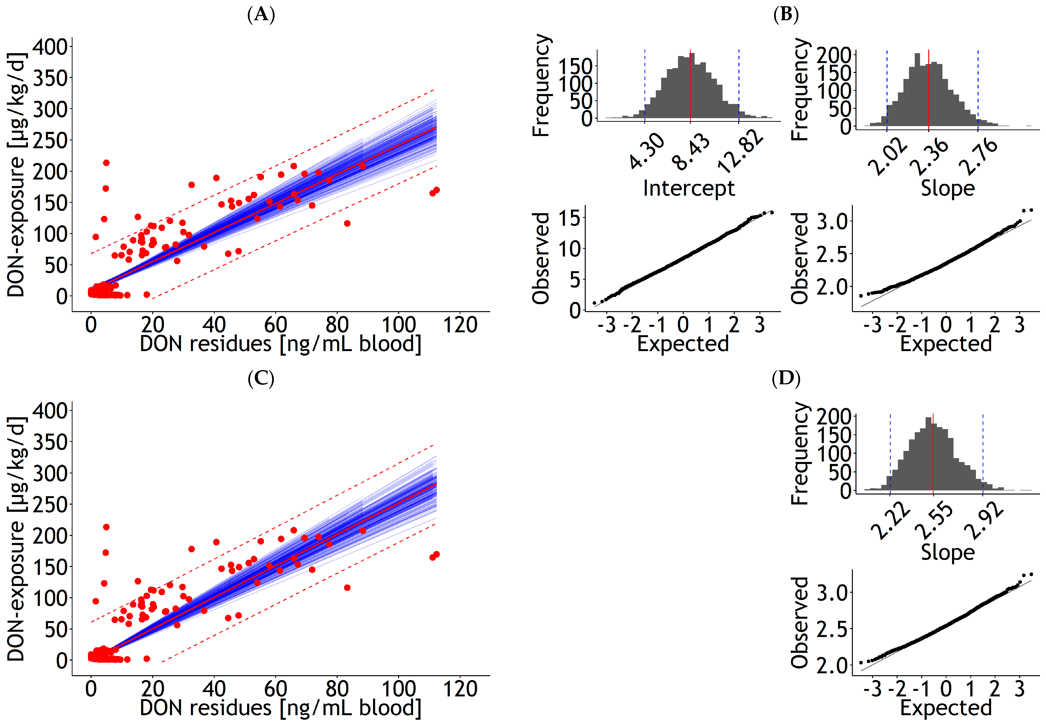
Development of Prediction Equations

The general evaluation strategy included comparisons of parameter estimations after bootstrapping of linear and robust linear regressions along with influential statistics to examine the effects of extreme observations. On the basis of the toxicokinetic consideration that non-detectable DON residues should be associated with no DON exposure, regressions were performed either with or without the intercept to investigate the effects of observations close to the origin, which might be differently influenced by LODs/LOQs for feed and physiological specimens.
In particular, DON residue levels in blood, urine, bile, and milk were each linearly regressed on DON exposure using the lm function of the package stats [17]. Prediction intervals were extracted from the regression results by the function predict.lm of the same package.
As linear regression employing ordinary least square (OLS) fitting is vulnerable to extreme observations, a robust fitting was additionally conducted by iterated re-weighted least squares (IWLS) using the rlm function of the MASS package [19]. The robust linear fitting puts less weights on influential observations, making regression results more robust compared with OLS estimations. In the next step, the validity of the regression coefficients obtained from the lm and rlm procedures was evaluated through the bootstrapping method. As a re-sampling method, bootstrapping does not rely on a known probability distribution; instead, it estimates the sampling distribution from which the means and standard errors are derived by the percentile method [20]. Regression coefficients were estimated from 2000 bootstrap replications; most researchers use this number, which is based on a sufficient accuracy to investigate regressions [21,22] and to ensure comparability in methodology. Distributions of regression coefficients were plotted as histograms for visual inspection, and mean values and standard errors were derived using the bootstraps procedure of the package rsample [23].
Linearity of trait relationships was additionally tested using the raintest function, which performs the rainbow test and is implemented in the package lmtest [24].
The above-described regressive methods were applied to all available matrices from Experiment 1 (blood, urine, bile, and milk) and Experiment 2 (blood). Slopes from those regressions generally provide information on the incremental increase in DON exposure per unit increase in DON residue levels in a particular matrix. A justification of a generalized application of derived regressions as prediction equations would be supported by comparable regression coefficients from independent studies. For this purpose, the relationships between DON residue levels in blood and DON exposures from Experiments 1 and 2 were further evaluated by a linear model, including DON exposure as the response variable, DON residues in blood as the continuous independent variable, the experiment number as a categorial variable, and the interactions between DON residues and experiment number using the lm procedure.
Indicators of influential statistics for regressions, such as Cook’s distance, hat score (leverage), and Studentized residuals, were evaluated using the augment.lm function of package broom [25].

Internal and External Validation of Prediction Equations for DON Residues in Blood

The ultimately derived prediction equation for DON residues in blood was used for internal and external validation. The corresponding regression coefficients were used to predict the DON exposure on the basis of DON residues in blood used for deriving the underlying prediction equation and from Experiment 3 for internal and external validation, respectively. The so-estimated DON exposures were linearly regressed on the corresponding observed DON exposures. As a number of predicted DON exposures of Experiment 3 were equal to zero, a Tobit model was additionally applied to these data, as OLS regression does not provide the best estimates for such censored data. The tobit function of the package AER was used for this purpose [26].
The precision and accuracy of these calibration lines were evaluated by the concordance correlation coefficient using the CCC function of the package DescTools [27]. Furthermore, concordance between the two methods was visually evaluated by the Bland–Altman method plotting the difference of corresponding data pairs, i.e., measured and estimated DON exposure, against their means [28]. The scatter of these data pairs was descriptively evaluated with the aid of horizontal helper lines, indicating the mean of the difference covered by the range limited by the ±1.96 standard deviation of that differences [28].

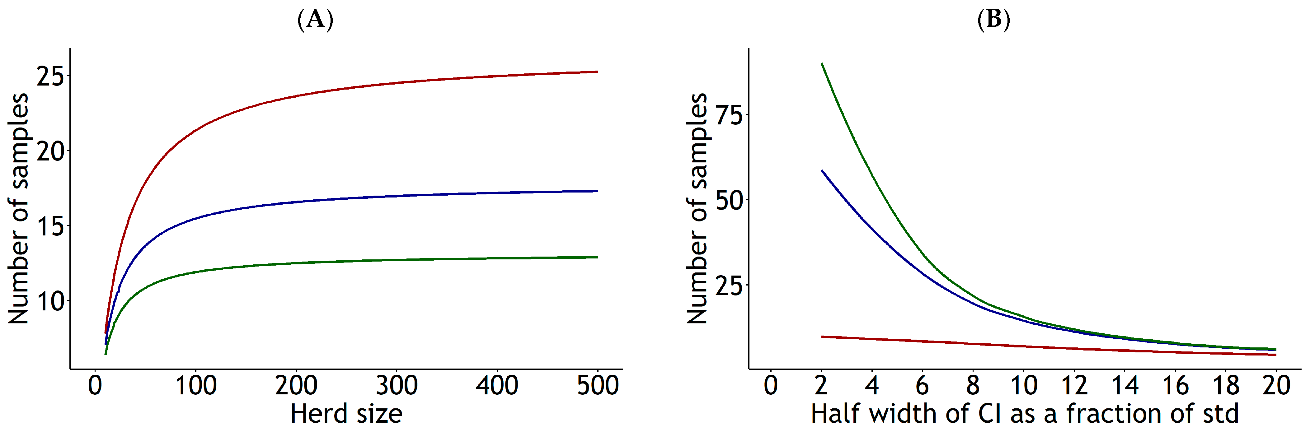
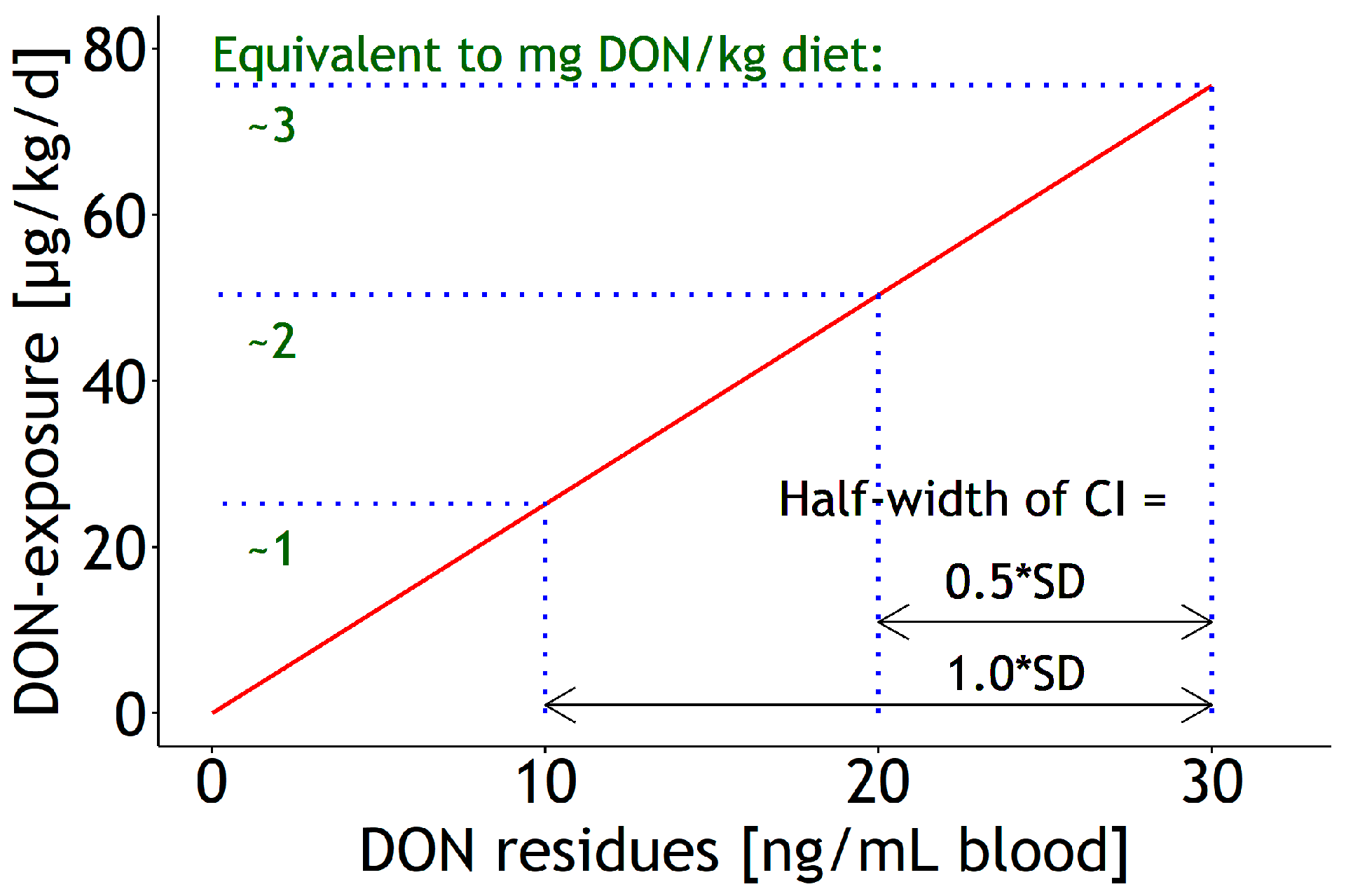
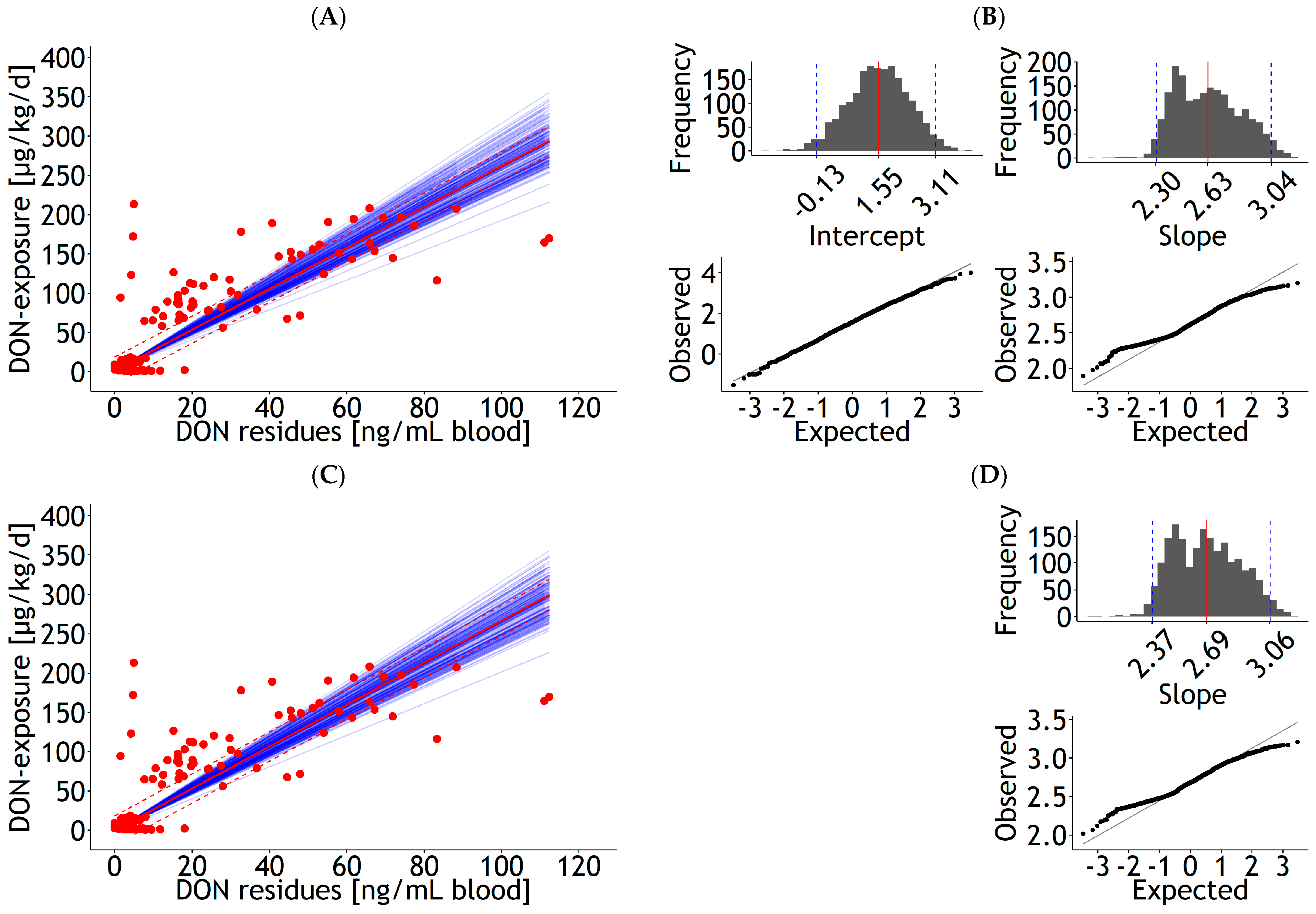
Estimation of Sample Size for Future Predictions

The definition of the confidence interval serves as a starting point for the planning of sample size for future predictions of the mean DON exposure ( y ¯ ) for a given herd size N. The width of the confidence interval of an arithmetic mean y ¯ depends on the variability of the trait expressed as the residual standard deviation s e , sample size n, and the t-quantile for a given confidence level P = 1 − α:
[ y ¯ s y ¯ t 1 α 2 ; n 1 ; y ¯ + s y ¯ t 1 α 2 ; n 1 ]   s y = s e n
Thus, the half interval width d is given as:
d = s y ¯ t ( 1   α / 2 ; n 1 )
and can be rearranged for n when the standard error s y ¯ is expressed through the ratio of the corresponding residual standard deviation s e and the square root of n:
n = t 2 ( 1 α / 2 ; n 1 ) s e 2 / d 2
The consequence of considering finite populations of the size N is that the standard deviation and, thus, the standard error of the mean for infinite populations are modified to:
s y ¯ = s e 2 n N n N
By considering this modified standard error for finite populations N, the sampling size can be derived through rearranging the half interval width d as [29]:
n = s e 2 d 2 t 2 ( 1 α / 2 ; n 1 ) + s e 2 N
The sample size must be determined iteratively since the t-quantile depends on the searched n.

3. Results

The goodness of fit for each different model was generally evaluated through the residual standard error (RSE) of the regressions rather than by r2 since the latter is not applicable for robust regressions.

3.1. Prediction Equations
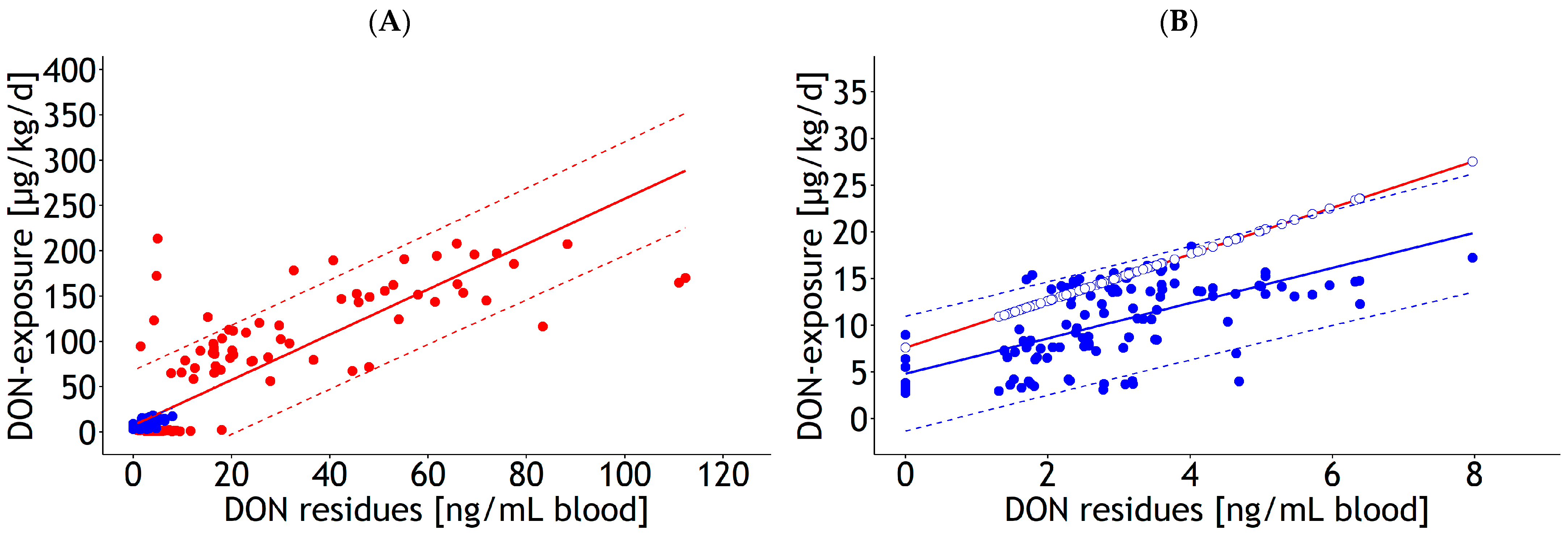
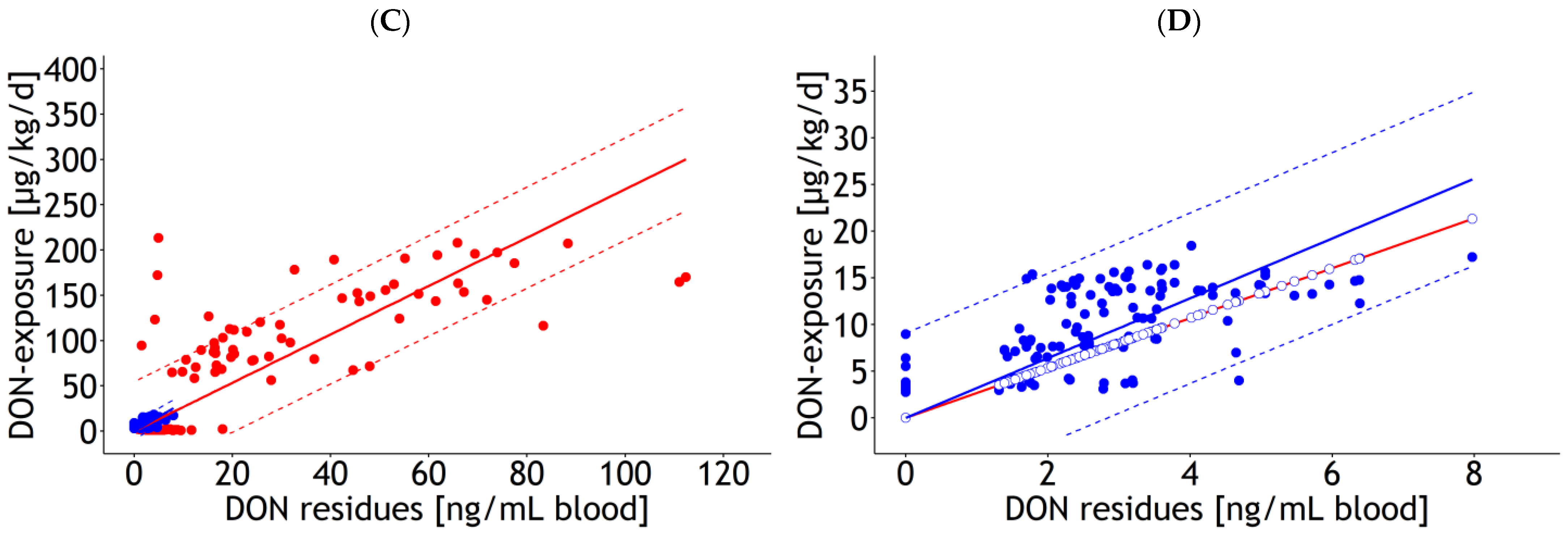
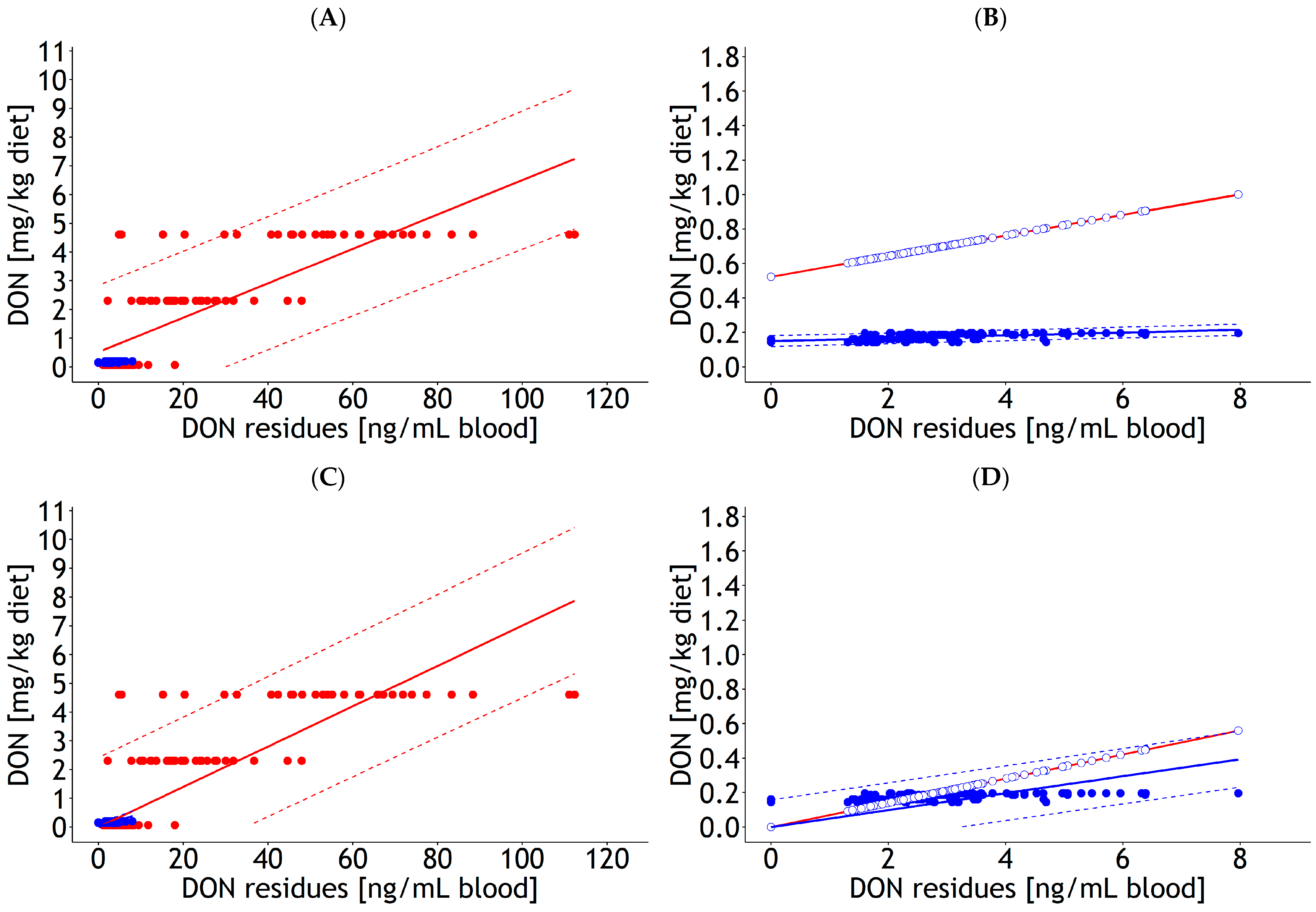
3.1.1. Blood

Separate regressions of DON exposure on DON residues in blood for Experiments 1 and 2 revealed positive intercepts on the ordinate that were significantly different from zero in both cases (p < 0.05; Figure A1, Table 2). Assuming that a DON exposure of zero would inevitably be associated with zero DON residue levels in blood, the intercept was omitted in a second step on the basis of these toxicological backgrounds. Due to such a redirection of positive intercepts on the ordinate towards to a zero intercept, the slopes became steeper. Due to forcing the regressions through the origin, the final minimum OLS and, consequently, the RSE became larger, albeit only slightly and at a generally higher level for Experiment 1 compared with Experiment 2 (Figure A1, Table 2).
In addition to separate simple linear regressions for Experiments 1 and 2, both datasets were additionally investigated through an analysis of covariance (ANCOVA) of the linear model, with DON exposure as the dependent variable. This ANCOVA demonstrated significant effects of the experiment as the categorial independent variable (p < 0.05) and of DON residues in blood as the continuous independent variable (p < 0.05) but failed to reach significance for the interactions between the experiment and DON residues (p = 0.827). The latter suggested that the slopes for Experiments 1 and 2 were not significantly different. For this reason, it was assumed that data from both experiments belonged to a similar population. Thus, data sets were combined for all further regressions to increase the number of observations used for deriving the final prediction equation. Regression of the joint dataset with and without an intercept, resulted, generally, in steeper slopes and suggested linearity, according to the rainbow test, when compared with the individual regressions. The height of the RSE was found to lie between those that were estimated separately for Experiments 1 and 2. The prediction interval and, consequently, the exposure threshold were tighter and smaller, respectively. Bootstrapping from the joint dataset resulted in a mean intercept with an ordinate of 8.43 and a slope of 2.36. The frequency distributions for both parameters suggest reasonable symmetry, and the corresponding intercept of 8.68 and the slope of 2.33 estimated for the original dataset were close to the corresponding bootstrapping means (Figure 1, Table 2). The qq-plot for the intercept suggested linearity over the entire range, while some departure from linearity was noticed at both ends. Interestingly, these deviations appeared less pronounced when the joint dataset was forced through the origin.
Robust linear regressions using the rlm function were performed in a similar way as described for the linear models employing the procedure lm. In general, robust regressions resulted in substantially lower RSE and correspondingly tighter prediction intervals and lower exposure thresholds. Moreover, slopes were steeper, and intercepts were estimated to be located closer to the origin (Figure A2 and Figure A3, Table 2).
Additionally, attempts were made to regress DON concentrations of diets directly on DON residues in blood while being aware that individual variation occurred only in the abscissa direction at the same time. For this reason, only lm procedures were tested (Figure A4 and Figure A5, Table 2).
The initial ANCOVA of the linear model for Experiments 1 and 2 for DON concentration in feed showed significant effects of the experiment as a categorical independent variable (p < 0.05) and of DON residues in blood as a continuous independent variable (p < 0.05) but did not reach significance for the interactions between the experiment and DON residues (p = 0.259), suggesting the experiment-specific slopes were not significantly different. Thus, datasets of both experiments were pooled for further regressions. Linear regression of DON residues in blood on DON concentration of the diets using the joint dataset resulted in a slope of 0.07, irrespective of regressing with or without an intercept. When an intercept was included in the model, it was estimated markedly lower when compared with the intercept when the data of Experiment 1 were regressed individually. As for DON exposure, the RSE of the regression using the combined dataset was lower than that resulting from the regression using Experiment 1 data only. The bootstrapping means for intercept and slopes reasonably matched those obtained from the regressions of the original datasets. The histograms suggested symmetric distributions, although the qq-plots displayed some deviation from linearity at both ends, particularly for the slopes.

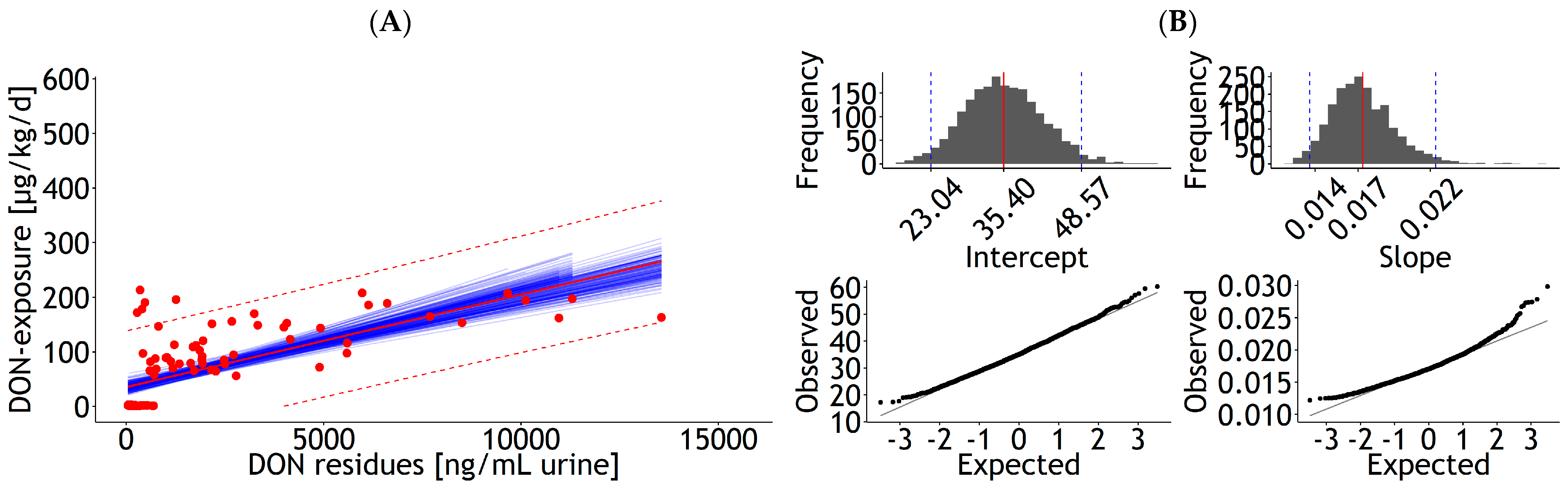
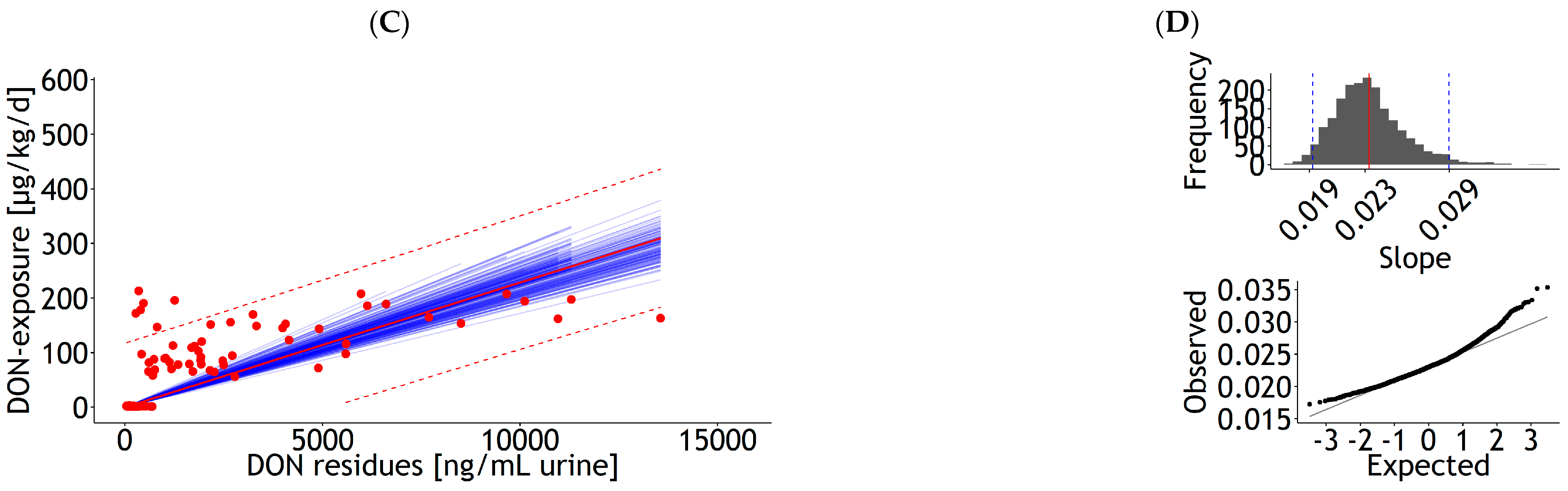
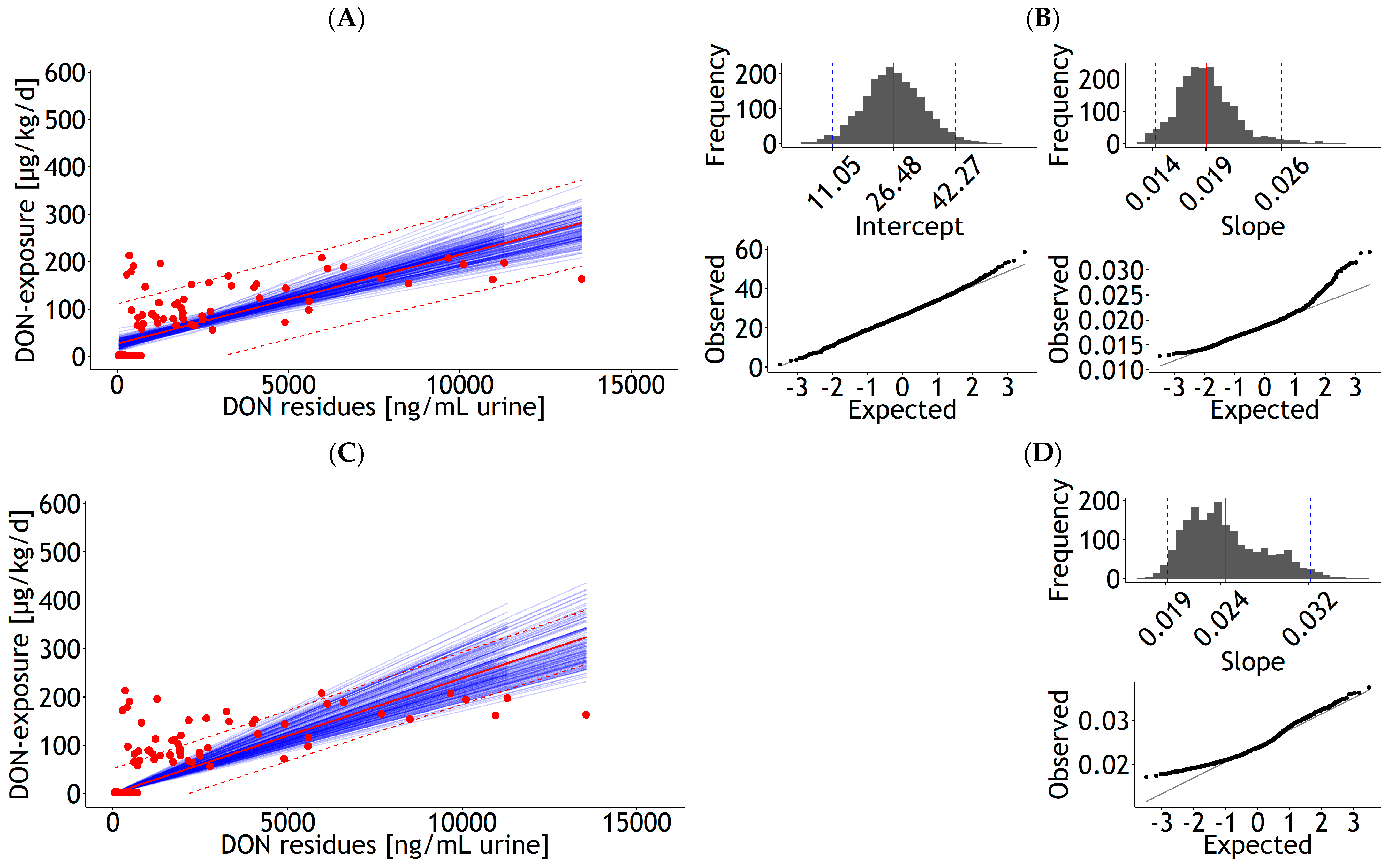
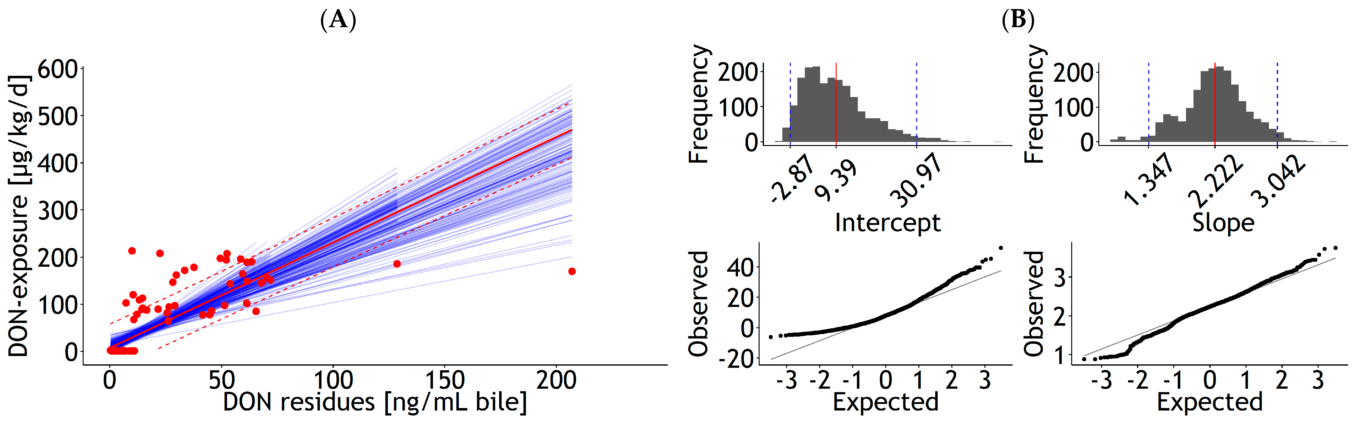
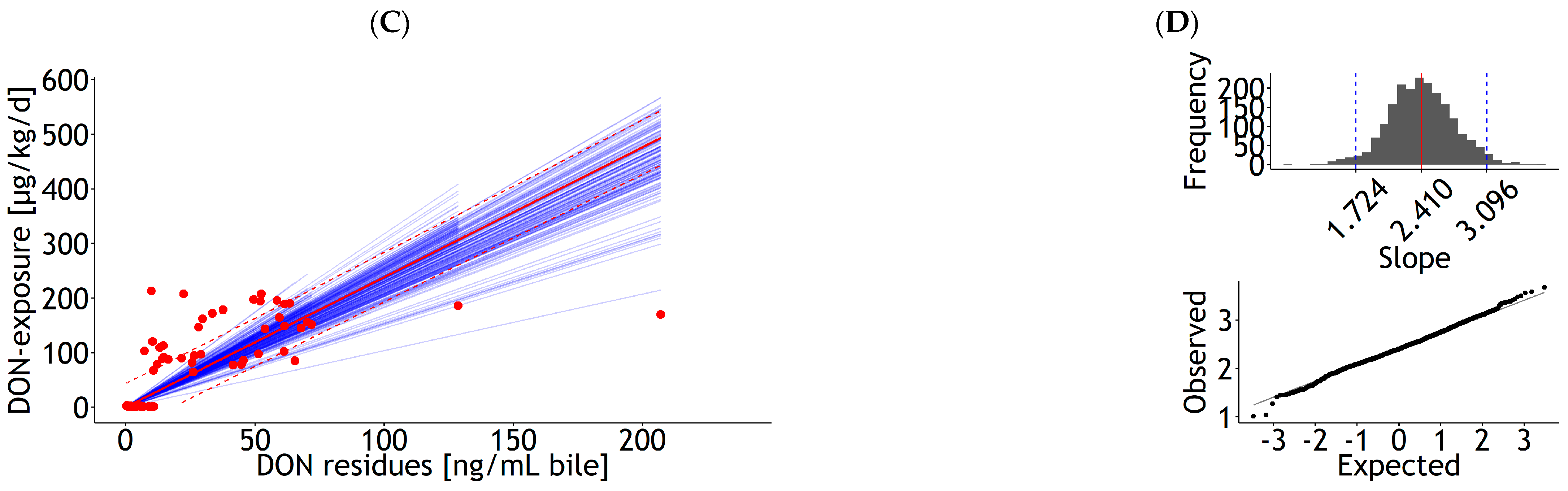
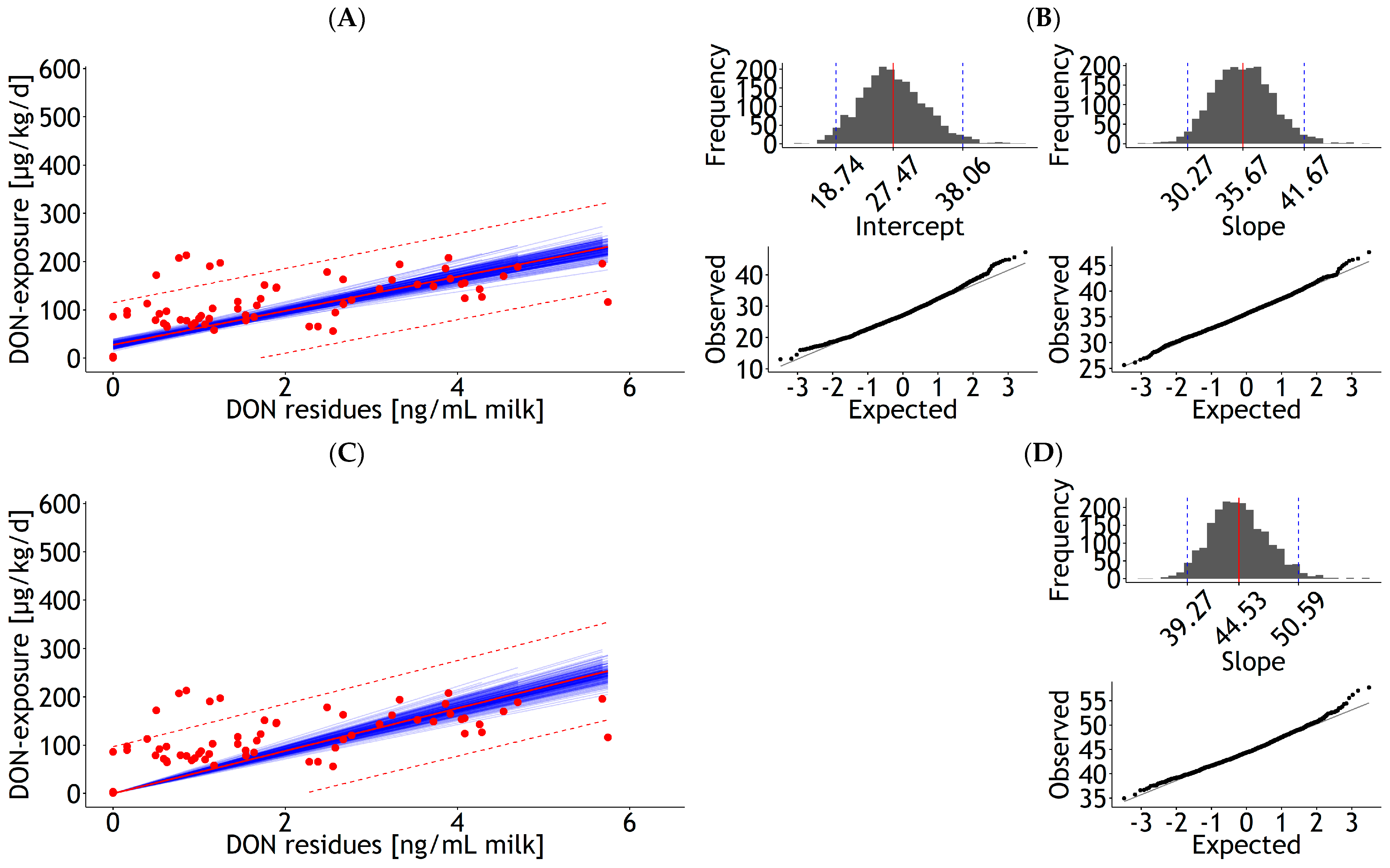
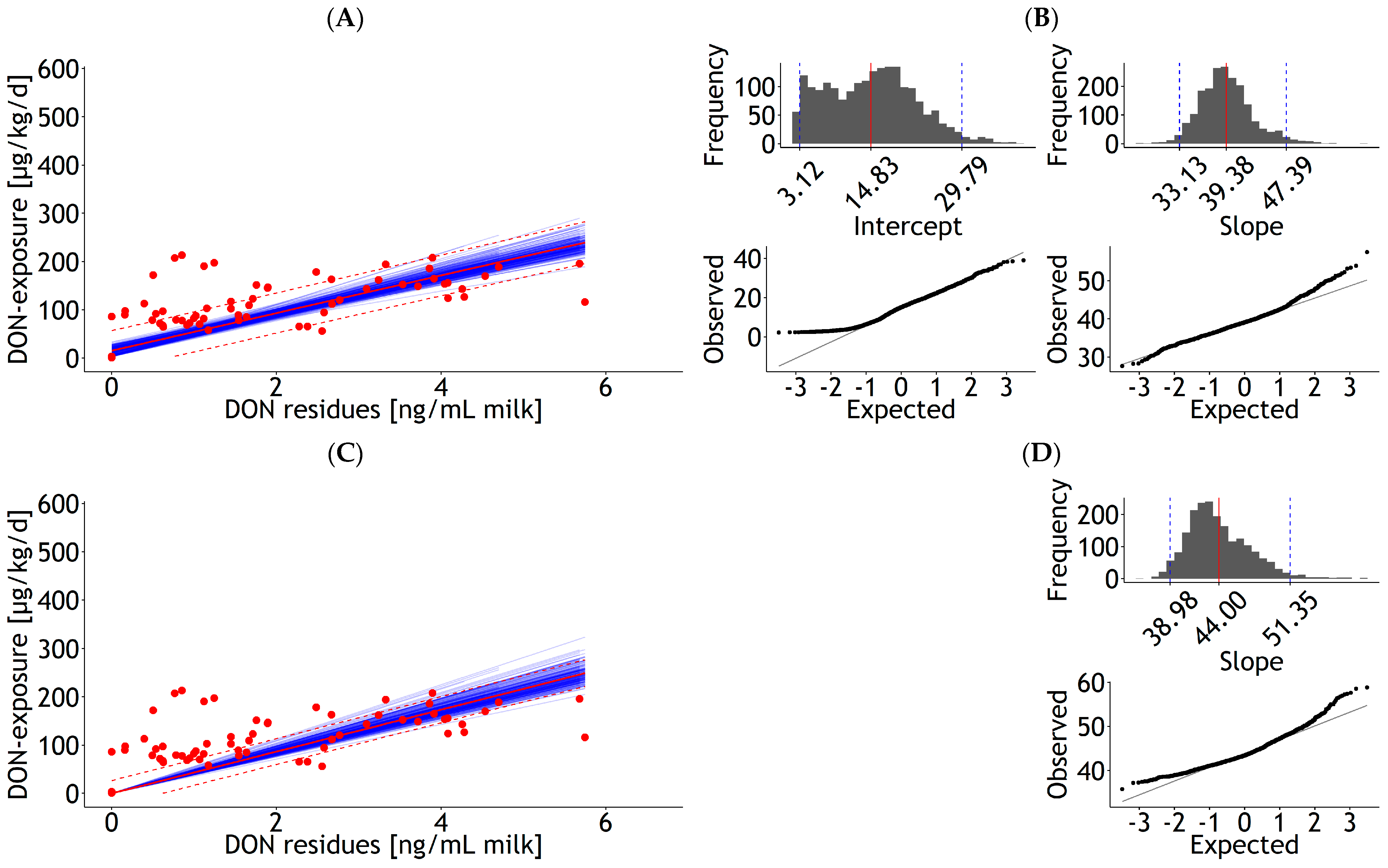
3.1.2. Urine, Bile, and Milk

Urine, bile, and milk samples were available from Experiment 1 only. Thus, lm and rlm were tested exclusively for these matrices (Figure A6, Figure A7, Figure A8, Figure A9, Figure A10 and Figure A11, Table 2). In general, for models with intercepts, those were significantly higher than zero, except for the rlm for bile. As for the blood models described, the slopes increased when the intercepts were omitted both for lm and rlm, albeit at a higher level for the latter. Although the bootstrapping means for intercepts and slopes matched those estimated from the original regressions for all three matrices both for lm and rlm, the histograms and qq-plots suggested departures from symmetry depending on the matrix and estimation procedure. While for urine and milk the lm procedure appeared to be superior to rlm, the opposite was noticed for bile.

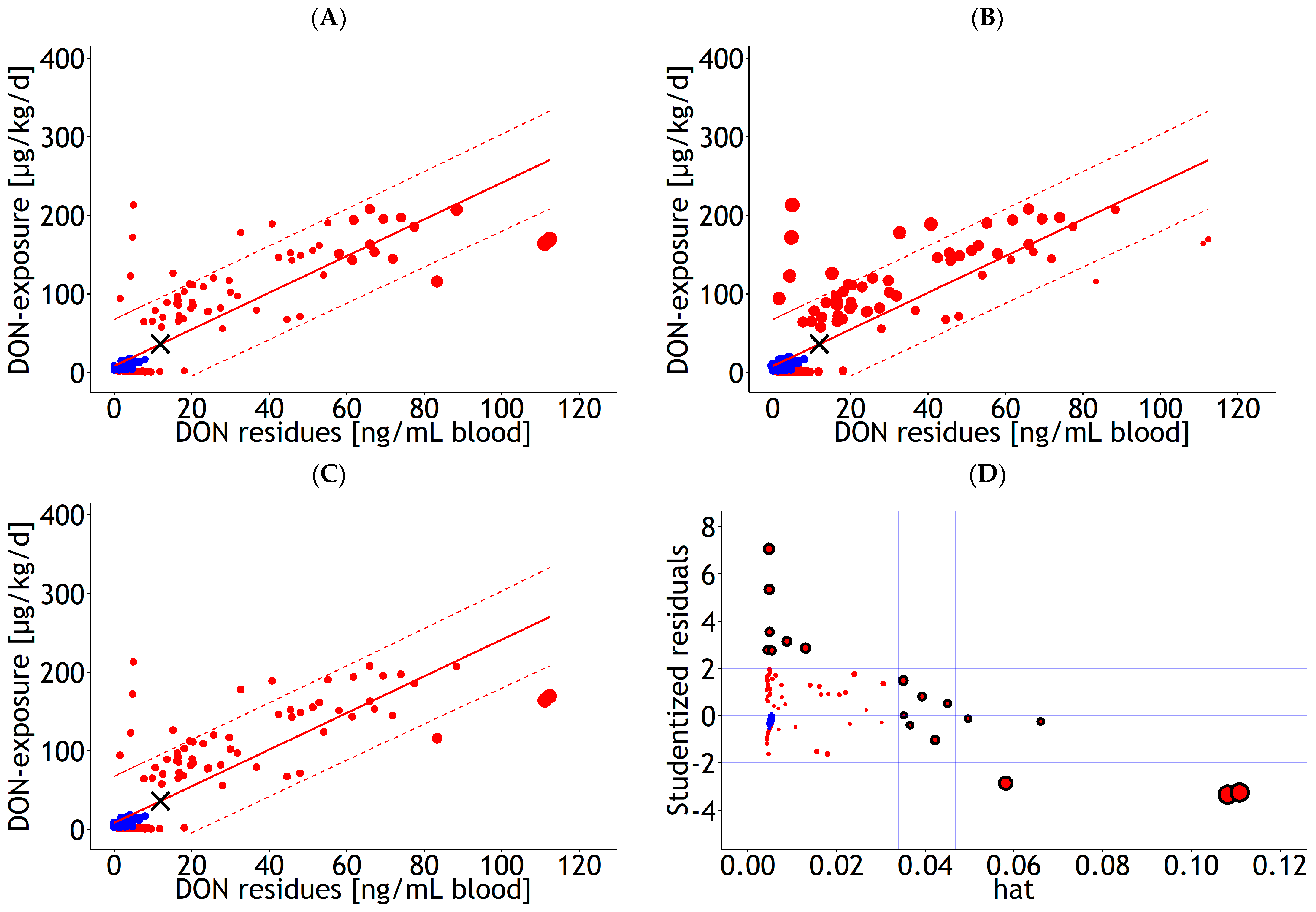
3.2. Influential Statistics

On the basis of a literature review, Chatterjee and Yilmaz [30] concluded that 25 or more regression diagnostic indices are known, many of which provide similar information. The authors recommended that three to five measures that are easily available from statistical software should be used. Amongst these five, the authors favored Studentized residuals, as they provide information on outliers; the hat values, as the diagonal elements of the hat matrix, they provide information on the influence independent of the value of the response variable; and Cook’s distance, which informs the change in parameter estimates.
Consequently, “suspicious” individual values were filtered using hat scores, Studentized residuals, and Cook’s distance. These influential indicators were evaluated for the final lm models without an intercept for the combined blood dataset (Figure 2) and the other matrices (data not shown). Hat scores for blood increased with distance from the centroid in the direction of the abscissa up to 0.11. A larger portion of the data of Experiment 1 were characterized by larger positive Studentized regression residuals compared with those with negative residuals. Only three observations located in the right part of the scatter showed larger Cook’s distances. Combining all 3 measures in 1 plot revealed that a total of 18 suspicious observations were identified, characterized by Studentized residuals that were either greater than 2; less than −2; had hat scores greater than the value represented by the mean of the hat scores plus the twofold standard deviation of the hat scores; or had a Cook’s distance larger than 1. Applying the same three filtering conditions to urine, bile, and milk revealed nine, four, and eight suspicious data points, respectively. In particular, hat scores varied from 0.01 to 0.18, 0.01 to 0.4, and 0.009 to 0.09; Studentized residuals ranged from −2.21 to 3.36, −3.17 to 3.39, and −2.55 and 3.73; and Cook’s distances ranged from ~0.0 to 0.54, ~0.0 to 7.07, and ~0.0 to 0.39 for urine, bile, and milk, respectively.

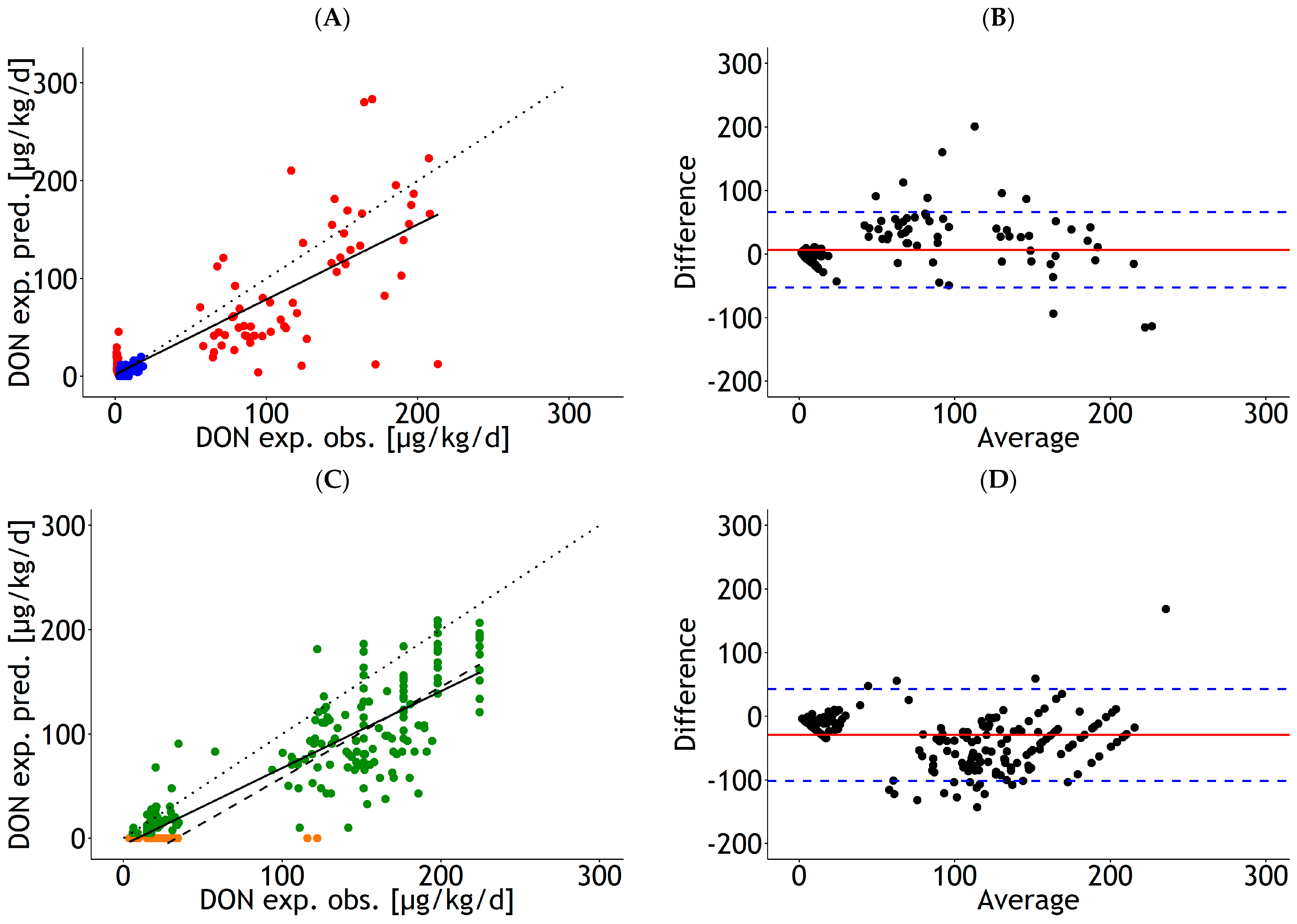
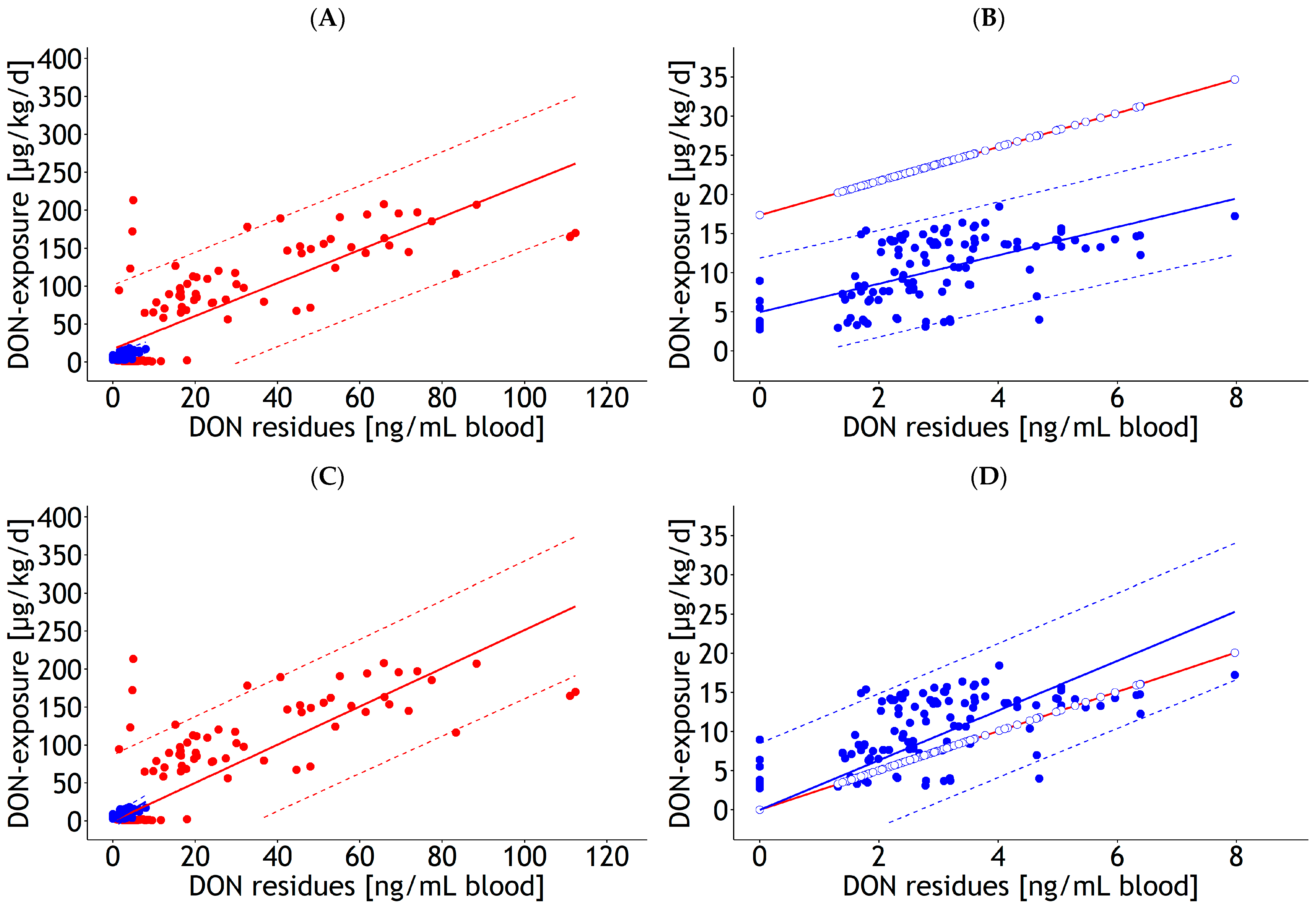
3.3. Internal and External Validation of Prediction Equations for DON Residues in Blood

Internal and external validations of Equation 6 were performed using the data from which the regression was estimated (combined dataset of Experiments 1 and 2) and data from an independent study (Experiment 3), respectively (Figure 3). The linear regressions for DON exposure predicted by Equation 6 on the observed DON exposure showed slopes less than 1.0 for both the internal and external validation (fig). Consequently, DON exposures were underestimated by 0.23 and 0.26 µg/kg BW/d per 1 µg/kg BW/d increase in observed DON exposure for internal and external validation, respectively. In the case of the external validation, the application of the Tobit regression to the data decreased this underestimation to 0.13 µg/kg BW/d. The Lin’s concordance correlation coefficient (CCC) of 0.83 and Pearson’s correlation coefficient (r) of 0.84 for internal validation as well as Lin’s CCC of 0.79 and Pearson’s r of 0.87 for external validation (full dataset, including left-censored data) demonstrated accuracy and precision less than 1 and supported the systematic underestimation of the predicted DON exposure, as indicated by the slopes of the linear regressions less than 1.0. The scale and location shifts were 0.91 and −0.12 for the internal validation and 1.18 and 0.42 for the external validation, respectively.
The Bland–Altman plots (Figure 3) demonstrate that the mean difference between the predicted and observed DON exposures nearly matched the zero-line for internal validation, but a systematic bias of −29.4 µg/kg BW/d was found for external validation. Bias did not systematically change with increasing mean values of predicted and observed DON exposures in either validation, and a total of 10 and 19 differences were identified to be located outside the ranges covered by the mean difference ± 1.96 standard deviation (limits of agreement).

3.4. Estimation of Sampling Size for Future Predictions

On the basis of the standard deviation of 20 ng DON residues/mL blood (Table 1), as determined for the combined dataset of Experiments 1 and 2, the half interval width of the confidence interval as a measure for precision requirements for sampling size estimation was expressed as a fraction of this standard deviation ranging from 0.1 to 1.0 or from 10 to 100%, respectively. On the basis of these prerequisites, the sampling sizes were iteratively estimated dependent on herd size ranging from N = 10 to N = 1000. It became clear that the required sampling size increased asymptotically with herd size and with lowering the half width of the confidence interval. The general interrelationships between these determining factors are shown in Figure 4, and specific numbers are provided in Abbreviations (HPLC—high-performance liquid chromatography; MS—mass spectrometer; UVD—ultraviolet detector; DAD—diode array detector; SPE—solid phase extraction; and IAC—immunoaffinity columns) and Table A2.

4. Discussion

Regression equations intended for future prediction of DON exposure or DON concentration of the entire diet dependent on DON residues in physiological specimens should be as easy as possible while still being statistically sound and based on toxicological backgrounds. The compromise between these requirements will be elaborated. As such, the consequences of variation in the observed data for future sampling size adequate to predict mean DON exposure as predicted by the estimation equations are discussed.

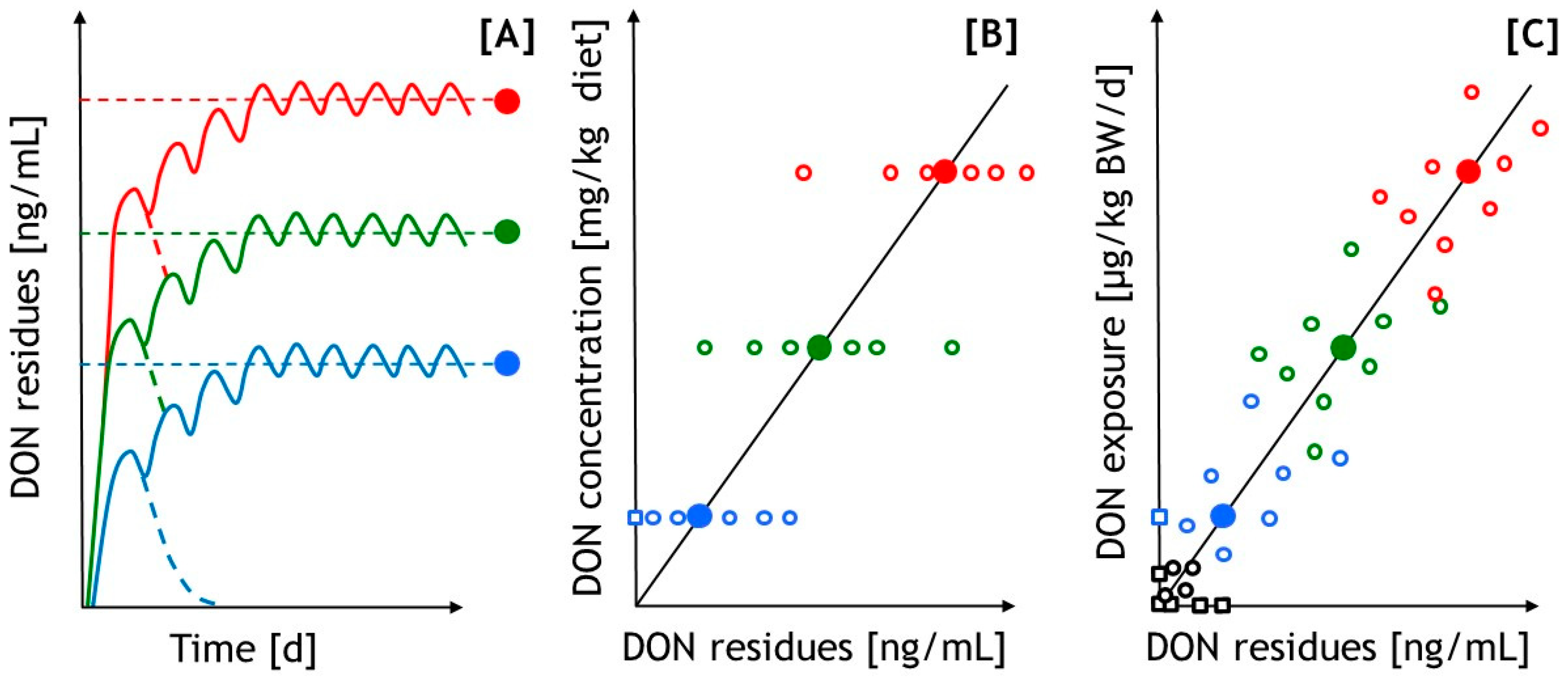
4.1. Toxicokinetic Aspects of DON as a Basis for Regressive Evaluation of the Data for Diagnostic Purposes

Prediction of oral exposure to DON by DON residues in physiological specimens requires a modellable relationship between the levels ingested and measured in those specimens. Simple positive Pearson correlation coefficients between 0.68 and 0.85 for the relationship between DON exposure and DON residue levels in urine, milk, bile, and blood suggest that inner exposure, as represented by the DON residues in those specimens, increases with oral DON exposure.
The nature of these relationships is basically related to all sub-processes of toxicokinetics, i.e., liberation of DON from the feed matrix in the digestive tract, absorption, distribution, metabolism, and elimination, and it can be either linear or non-linear, which has consequences for the modelling strategy. The levels of a drug or toxin in the blood depend on the dosage regimen or exposure scenario, respectively. The time vs. blood concentration profile of a multiple oral drug administration regimen is characterized by an initial increase until a steady state is reached [31] (Figure 5). The oscillation of plasma drug concentrations at a steady state depends on the half-life of the drug and the length of the administration interval [31]. Intuitively, a comparable situation might be assumed when cows consume a DON-contaminated total mixed ration (TMR) over a certain period of time. Here, the shape of the DON residues in blood at a steady state depends mainly on the meal size and meal frequency, representing the dose and administration intervals, respectively. When TMR is offered for ad libitum consumption, the meal frequency varies, for example, between 31 and 56 bouts/day depending on diet type, whereby meal intervals are not equidistant, and meal sizes fluctuate between 0.4 and 0.7 kg/bout [32]. Therefore, the oscillation of DON residue concentrations in blood at a steady state, as depicted in Figure 5, is an idealized one but will differ in magnitudes for peak and trough levels among individual animals depending on their eating behavior. The level of the mean steady state concentration of DON residues in blood is assumed to be dependent on the total oral dose, which, in turn, is related mainly to the dietary DON concentration. This situation is similar to drugs where an increase in dose linearly increases the drug concentration in blood at a steady state [31] for non-accumulating drugs. A similar situation might be assumed for DON, which is rapidly absorbed and eliminated both in non-ruminants and in ruminants without being accumulated [7]. Indeed, linear relationships between DON exposure and DON residue levels in blood were demonstrated for wethers [33], Holstein bulls [34], and dairy cows, which were re-evaluated in the present study.
On the basis of these theoretical considerations, the relationships between DON residue levels in physiological specimens and DON exposure were generally assumed to be linear. Therefore, exclusively linear models of regression were evaluated, and apparent departures from linearity were traced back to toxicokinetic features of DON becoming apparent in the available datasets, reflecting a practical exposure scenario.
If it is further acknowledged that a zero exposure to DON should not result in any DON residues in a physiological specimen, the linear regression line is supposed to intercept the origin. On the basis of this theoretical background, the linear regression models without an intercept are supposed to reflect the toxicokinetic situation more reliably, irrespective of the fact that the intercepts were significantly different from zero in most cases when estimated for comparative purposes (Table 2). Difficulties in matching the origin when intercepts are estimated result from the aspects depicted in Figure 5 and can be partially traced back to differences in the LOD/LOQ between feed and physiological matrix (Table A1), resulting in either DON residues or DON exposures intercepting the ordinate and abscissa, respectively. Such situations occur particularly when diets with (low) background DON contaminations are fed and inevitably cause noise in the region of origin. To counteract this methodological noise, the regression models forced through the origin (i.e., models without an intercept) are supposed to reflect the real situation in this region more reliably, although a slight loss in statistical power and, consequently, a broadening of the prediction interval have to be accepted at the same time.

4.2. Handling of Influential Observations and Fitting Methods

Influential statistics evaluate the effects of (suspicious) observations on the results of the regression analysis [35]. The general strategy is to examine the consequences on regression coefficients when such observations are omitted. Standardized measures that employ this approach are hat scores (hat values, leverages), Studentized residuals, and Cook’s distance, and they allow comparisons across different regressions [35].
If the residual of an observation obtained from an OLS fitting with this observation is small compared with its residual resulting from an OLS fitting without that observation, then its hat score is high. Hat scores vary between 0 and 1 and are evaluated differently. Common to all definitions for setting limits for separating suspicious observations is that they are based on rules of thumb. While some recommend setting the limits at 2 to 3 times the mean hat score [36,37], others set the limit at mean value of the hat scores plus the two- to threefold standard deviation of the hat scores [38]. The Studentized residual of an observation increases as the residual itself increases, and it is regarded as critical when it becomes greater than two or less than negative 2. Cook’s distance combines Studentized residuals with hat scores and increases when both influential measures increase. Observations with Cook’s distances greater than 1 are expected to have significant effects on the regression coefficients [35]. All these influential measures can only aid in identifying observations that behave differently from most other observations. It is generally agreed that the experimenter has to decide whether these suspicious observations are indeed outliers or explainable observations to be retained in the data. In the present study, none of the 18 identified suspicions observations originating exclusively from Experiment 1 could be traced back to experimental, pre-analytical, or analytical errors. Rather, their suspicious deviation from the scatter of most other observations might be due to toxicokinetics, as discussed above and further elaborated here. On specimen collection days, cows were sampled between ~8:00 and ~13:30 without noting the exact clock time. On the basis of this time span of approximately 5.5 h and on the automatic recording of the time of the last meal prior to the beginning of sampling at 8:00, the real time span between the last meal of a cow and the sampling of blood and other specimens varied between less than 20 min for cows that were coincidentally taking a meal when picked up for sampling and more than 10 h when the last meal was taken on the evening before sampling. Additionally, meal sizes for the last meals before sampling varied between 0.1 and ~5 kg fresh matter TMR. Furthermore, taking into account the rapid absorption and elimination of DON in dairy cows, as indicated by blood peak times of 3.5 h and 4.7 h, and an estimated elimination half-life of approximately 2.5 h to 3 h [39] after a single oral DON bolus, it is likely that individual cows of similarly calculated DON exposures exhibited large differences in DON residue levels, reflecting rather the kinetics observable after a single DON bolus than that at the postulated steady state. In fact, the minimum and maximum values of 1.0 and 18.0 ng/mL, 2.5 and 48.0 ng/mL, and 4.8 and 112.3 ng/mL for the low, medium, and highly DON-exposed groups of Experiment 1, respectively, support a departure from the steady state conditions. Nevertheless, most observations followed the postulated linear pattern, which was confirmed by the rainbow test, particularly when the combined dataset of DON residue levels in blood from Experiments 1 and 2 was used for the regression. However, the apparent departures from linearity observed for some regression equations are likely caused by the discussed noise in the region of the origin and by the fact that lower toxin concentrations both in the diets and the physiological specimens are associated with larger unavoidable errors, according to the rules of Horwitz [40]. While linearity can be assumed for DON residues in blood on the basis of toxicokinetic backgrounds, the situation for the other specimens appears to be more complex. Urine, bile, and milk are the main excretory routes for DON residue elimination but are excreted irregularly (bile and urine) or with an artificial pattern (milk). Thus, DON residues are more or less concentrated in these matrices depending on the magnitude of influx from the blood, which, in turn, depends on the time elapsed since the last meal and its size. Although these factors contribute to the variation, linearity was also confirmed for the regression equations estimated for urine and milk, while DON residue levels in bile obviously did not follow a linear pattern, according to the rainbow test. A closer look at the scatter of bile residues revealed that two observations in particular that were located in the right lower quadrant were flagged as influential. In fact, the maximum DON residue concentration in bile was the only observation amongst all matrices that exceeded a Cook’s distance of 1 and reached a value of 7.07. Bootstrapping of the linear models resulted in two-peaked slope distributions and substantial deviations from linearity in the qq-plots. In this situation, bootstrapping of the robust linear regression largely overcame these problems, leading to a symmetrical slope distribution, particularly when estimated without an intercept. Moreover, the differences in the slopes estimated through linear and robust linear regression were larger for bile than for the other matrices. Larger differences in regression results obtained from OLS fitting vs. IWLS, as observed for bile, provided a practical diagnostic warning that outliers may be influencing the OLS results [41]. That this was observed only for bile, although even more individual observations were flagged as apparently influential in other matrices, might be due to the fact that extreme values occurred both in the direction of the abscissa and the ordinate, which was not the case for bile. This might also be the reason why the robust fitting of milk DON residues using bootstrapping even deteriorated the symmetry of slope distribution and the corresponding qq-plot. The same phenomenon was observed for blood DON residues, where OLS was found to be superior compared with IWLS. A similar trend was noticed for urine.

4.3. Comparative Aspects on Suitability of Various Matrices as Predictors

In addition to the discussed toxicological and statistical features, particularly practical aspects need to be considered to decide which matrix is preferred for the diagnosis of DON exposure (Table 3). The inner exposure to DON is best reflected by blood since it transports DON residues directly to target tissues. Only fractions of systemically absorbed DON residues are extracted from blood and finally excreted via urine or milk, whereas DON residues in these specimens are less related to the levels in target tissues on theoretical backgrounds. The same is principally true for bile, but closeness to inner exposure is further compromised by a putative, but up to now not quantifiable, enterohepatic cycling of DON residues, although comparable ranges of DON residues in blood and bile suggest at least a less pronounced role of such a cycling as compared with ZEN residues. These aspects further support the discussed problems in fitting DON residues in bile to linear models. Thus, the relationship to dietary DON exposure is rated as less linear than that for blood, urine, and milk.
In addition to these toxicological and statistical aspects, analytical issues and practicability of the sample collection need to be balanced with the former aspects for a decision on a particular specimen. Particularly when it comes to exposure assessment at background DON contamination of feed, rather low LODs/LOQs are required both for feed and for physiological samples to avoid the decision of how to handle analytical results which are lower than LOD (results might set to zero, to the value of the LOD, or to the half of the value of the LOD for further calculations) or higher than LOD but lower than LOQ (values are generally regarded as questionable but are sometimes used for further statistical analyses). All these uncertainties cause the discussed noise in the region of the origin, consequently causing predictive uncertainty. Comparing the LODs/LOQs with the respective ranges detected in various matrices (Table A1 and Table 1), particularly at lower dietary exposure levels, would clearly favor urine, where rather large DON residue concentrations that are safely detectable can be expected. Moreover, the sampling of urine is non-invasive but might require more time than the sampling of blood, milk, or even bile. Milk sampling, on the other hand, could be implemented in the daily milking routine but is hampered by the lowest DON residue concentrations. Blood and bile can be sampled by a simple puncturing of a blood vessel or of the bile bladder, respectively. While puncturing of a Vena jugularis externa can be accomplished with a routine diagnostic tool, the sampling of bile requires an ultrasound-guided localizing and puncturing of the bile bladder situated at the right abdominal wall (Figure 6). Although prediction equations based on DON residues in bile need to be qualified further, the collection of bile could be interesting when monitoring ZEN exposure at the same time. ZEN and its metabolites undergo an intensive enterohepatic cycling, whereby diagnostic opportunities are likely better than for DON. DON and ZEN often co-occur in maize-based feedstuffs commonly used in cow feeding. Therefore, analytical methods for detecting DON and ZEN residues at the same time, as applied in Experiments 1 and 2, make bile interesting as a diagnostic specimen.

4.4. Internal and External Validation of Prediction Equations for DON Residues in Blood

A simple Pearson correlation coefficient and the r2 of a corresponding linear regression are unsuited to confirm the concordance, defined as the degree of agreement, between two methods, as they can still deviate systematically from each other [22,42]. Pearson’s r just reflects the precision component of the linear relationship and is a measure of how far the observations are located from the best-fit line, while accuracy considers how far the best-fit line deviates from the 45° line [43]. Precision and accuracy are combined in the CCC as proposed by Lin [43]. Furthermore, it is strongly recommended to estimate the intercept in addition to the slope of the regression line as an essential part of an overall (fully quantifying) calibration as a regressive form of validation of the known (measured) DON exposure. Thus, the calibration curves for internal and external validation were estimated with intercepts. The intercept for the internal calibration line did not significantly differ from zero, while the slope suggested that the predicted DON exposure was 0.23 µg/kg BW/d lower per each 1.0 µg/kg BW/d increase in observed DON exposure, which is equivalent to a 23% underestimation. The smaller location shift compared with the larger scale shift further substantiated the systematic deviation of the regression line from the 90° angle bisector. The closer both shifts are to zero, the more closely the regression line will match the 45° line and CCC will reach 1.0 when both shifts are equal to zero [44]. Compared with the internal calibration, both shifts were higher for the external calibration, whereby the slope nearly reached that estimated for the internal calibration curve, resulting in an underestimation of 26%. For a number of observations (n = 80) of the dataset used for external validation (Experiment 3), the predicted DON exposure was zero, although a positive DON exposure was noticed at the same time, which likely resulted from the more than tenfold higher LODs for DON residues in blood compared with Experiments 1 and 2. OLS fitting does not provide the best estimates for regression coefficients when dependent observations are equal to zero, for example, such as when they are left-censored, while Tobit regression uses a modified likelihood function in such a way that it mirrors the unequal sampling probability for non-censored and censored observations [45]. Applying this method to Experiment 3 increased the slope from 0.77 when estimated using OLS to 0.87 when using Tobit regression. At the same time, the intercept on the ordinate decreased markedly to a value −29 µg DON/kg BW/d and, consequently, had a more pronounced location shift. Moreover, the RSE was higher compared with OLS fitting. On the basis of this and for a better comparability with the internal validation, the results of the OLS were preferred.
CCCs were comparable and reached 0.83 and 0.79 for internal and external non-Tobit OLS calibrations, respectively. Assigning the height of the CCC to the categories of poor, excellent, or further is handled differently in the literature [46]. If the CCC is interpreted in a similar way to Pearson’s r, as suggested by [47], then the CCCs for both internal and external validation are rated as moderate to very strong, depending on the author, as reviewed in [46]. Nonetheless, the decision of whether the degree of agreement is sufficient largely depends on the professional context. A further evaluation of agreement between two methods is possible when the differences between the corresponding data of the two methods to be evaluated are plotted against their means (Bland–Altman plots). Compared with correlation or regression plots, with this type of plot, the size of the differences are easily evaluable; the distribution around the zero line can be assessed, and it can be evaluated whether the differences increases with means [47]. The mean difference is regarded as an estimate of the average bias of one method relative to the other one [47]. For the current data, the bias differed only slightly from zero for the internal validation but to a larger extent for the external validation. Here, the bias of 29 µg DON/kg BW/d would correspond to an underestimation of approximately 1 mg DON/kg diet through the prediction Equation 6 (Table 2) when extrapolated to DON concentration in feed. In addition to the overall bias, the evaluation of how individual observations agree for the two methods can be managed by using the standard deviations for constructing the limits of agreement as ±1.96 standard deviation of the differences. Thus, approximately 95% of the observations are expected to be within the limits of agreement when a normal distribution is assumed. That this assumption holds true for both internal and external validation might be deduced from the homoscedastic scatter. The observations located outside the limits of agreement are those considered as possible influential observations, which, were discussed as valid data from a toxicokinetic viewpoint and, thus, were not omitted from the regression analyses. At the same time, these observations cannot, or can only poorly, be predicted. In addition to the toxicokinetic issues already discussed for these observations, the dilemma with these data might also be caused by the method of calculating the DON exposure and the timing of the individual blood sample assigned to this exposure. DON exposure represents the daily mean value, while the blood sample was collected at a specific timepoint on that particular day, matching the average DON exposure more or less.
Taken together, the Bland–Altman plots suggested a reasonable agreement between measured and predicted DON exposure for internal validation, while a systematic underestimation was noticed for the external validation, whereby a generalization of prediction Equation 6 is questioned. However, Bland and Altman [28] suggested a correction for this bias. This would entail adding a constant value of 29 µg DON/kg BW/d to the predicted DON exposures based on Equation 6, irrespective of the level of DON residues detected in the blood. Further data should be generated for external validation. Except for the bias that was not revealed by the Bland–Altman method, the validation results for external and internal calibration were reasonably comparable, although different analytical methods were used for the detection of DON residues in the blood.

4.5. Recommendations for Appropriate Sampling Sizes for Future Predictions

Assessment of DON exposure based on DON residues in physiological specimens aims at differential diagnostics of clinically ill individual cows or at a general evaluation of the herd exposure level. For the latter, one is interested in the mean expected exposure level as a basis for management measures. For matching this mean exposure to a defined statistical confidence, it has to be determined how many cows need to be sampled. This, in turn, depends on the expected standard deviation of DON residues, e.g., in the blood, as a predictor for DON exposure on herd size and on statistical confidence, which can be influenced by setting an appropriate half width of the confidence interval. Standard deviation of DON residues in blood obtained from the pooled datasets of Experiments 1 and 2 (Table 1) was used as a starting point for defining the half width of the confidence interval as a proportion ranging from 0.1 to 1.0 or from 10 to 100%. The decision regarding an adequate half interval width must be derived from a professional viewpoint, i.e., to decide whether the associated precision is low or high from a practical viewpoint. For example, assuming the half interval width of the confidence interval to be onefold that of the standard deviation of 20 ng DON residues/mL blood places it between 10 and 30 ng/mL (Figure 7), which corresponds to an estimated mean of 20 ng DON residues/mL blood. This would correspond to a range of DON exposures between 25 and 76 µg/kg BW/d when Equation 6 (Table 2) is used for prediction.
This range can be even better evaluated when the exposure is traced back to the diet contamination with DON. This requires an assumption regarding feed intake and BW. Assuming a DMI of 20 kg/d and a BW of 700 kg would correspond to a dietary DON contamination range of 2 mg (1 to 3 mg/kg) at a reference DM content of 88%, which is clearly independent of the real DON residue levels. Taking further into account that 5 mg DON/kg diets are considered as critical for dairy cows, a range of 2 mg DON/kg diet would be regarded as too imprecise for the expected mean value. Reducing the half width of the confidence interval to 0.5 times the standard deviation would result in a range of 1 mg DON/kg diet as a measure for precision for the associated mean value. The reduction in the half interval width of the confidence interval from 1 to 0.5 times the standard deviation would correspond to requiring 9 additional cows to be sampled for a herd size of 100 cows, i.e., 15 cows vs. 6 cows (see Table A2), which is the price for the improvement in precision.

5. Conclusions

The fluctuation of DON residues in blood and other matrices needs to be examined frequently in the course of the day along with the times and sizes of meals relative to sampling in order to substantiate the expected steady state conditions claimed for ad libitum fed cows, which, in turn, is the toxicokinetic basis for the assumed linearity. In addition to linearity, the assumption was made that zero DON residue levels in physiological matrices cannot be associated with a significant DON exposure. Therefore, linear models without intercepts were preferred.
IWLS fitted models (robust regressions, rlm models) generally resulted in lower RSEs and tighter prediction intervals through the outweighing of apparent outliers. However, on the basis of toxicokinetic considerations, these outliers were identified as valid observations. Together with the overall variability in the data, OLS-fitted models (ordinary linear regressions, lm models) were considered as more appropriate. The associated wider prediction intervals appeared to reflect the practical situation more reliably. Furthermore, bootstrapping of IWLS and OLS models was used to avoid having to rely on the assumptions that usually have to be fulfilled for regressions. Results showed that OLS fitting was superior compared with the corresponding IWLS fittings, except for the case of bile. On the basis of the limited data situation for bile, the derived equations should only be used with caution.
On the basis of the above concluded assumptions and limitations, Equation 6 is recommended for blood, Equation 20 for urine, and Equation 28 for milk. On the basis of both internal and external validation, blood is currently the most trustworthy for prediction of DON exposure, and the use of larger sets is recommended.
Models directly relating DON residues in blood to the DON concentration in the diet are the models of choice, as the DON concentrations in the diet can be associated with established critical concentrations, while predicted DON exposures need to be transformed to DON concentrations of the diets by assuming a particular BW and DMI. Although Equations 13 to 16 are based on DON concentrations of the diets as a response variable, their validity might be hampered by left-censored data, limiting the validity to only a few levels. More graded DON levels should be tested to improve these equations.
For DON residue levels in physiological matrices which are lower than the exposure thresholds, an unknown proportion of future predictions will result in a zero DON exposure, although the best estimate is located on the regression line and will, consequently, predict positive DON exposures. In other words, DON residue levels larger than the exposure threshold predict positive DON exposures lying within the prediction interval with a 95% probability.
With regard to sampling size for future predictions of the mean exposure of a given herd size, the standard deviation and half width of the confidence interval are the determining parameters. Pooling of the collected samples to one individual sample to be analyzed for DON residues is not recommended since extreme individual values are assumed to adulterate the mean value and, consequently, the predicted DON exposure. Individual predictions are loaded with a large portion of uncertainty, as was evident by the width of the prediction intervals.

Author Contributions

The study was designed and conceptualized by S.D.; methodology was developed by S.D., J.S. (Joachim Spilke) and A.S.; resources were researched by S.D.; curation, preparation, and visualization of the data was conducted by S.D., S.K., F.B., A.S. and J.S. (Janine Saltzmann); writing—original draft preparation and writing—editing were performed by S.D. All authors have read and agreed to the published version of the manuscript.

Funding

This research received no external funding.

Institutional Review Board Statement

Not applicable since no experiment was carried out for the present study.

Informed Consent Statement

Not applicable.

Data Availability Statement

Data sharing not applicable. No new data were created in this study.

Conflicts of Interest

The authors declare no conflict of interest.

Appendix A

Figure A1. Linear regression (method lm) of deoxynivalenol (DON) residues in blood on DON exposure with ((A,B) for zooming in the lower concentration range) and without intercept ((C,D) for zooming in the lower concentration range) separately for Experiments 1 and 2 (n = 116 and n = 121, respectively). Red and blue solid lines denote the linear regressions, and dashed red and blue lines limit the prediction intervals at a 0.95 confidence level for future predictions for Experiments 1 and 2, respectively. Red and blue filled dots show the corresponding measured data pairs. Blue open circles lying on the red solid line represent the predicted values of Experiment 2 when regression of Experiment 1 is used as prediction equation.
Dairy 04 00024 g0a1
Figure A2. Linear regression (method rlm) of deoxynivalenol (DON) residues in blood on DON exposure with ((A,B) for zooming in the lower concentration range) and without intercept ((C,D) for zooming in the lower concentration range) separately for Experiments 1 and 2 (n = 116 and n = 121, respectively). Red and blue solid lines denote the linear regressions, and dashed red and blue lines limit the prediction intervals at a 0.95 confidence level for future predictions for Experiments 1 and 2, respectively. Red and blue filled dots show the corresponding measured data pairs. Blue open circles lying on the red solid line represent the predicted values of Experiment 2 when regression of Experiment 1 is used as prediction equation.
Dairy 04 00024 g0a2aDairy 04 00024 g0a2b
Figure A3. Linear regression (method rlm) of deoxynivalenol (DON) residues in blood on DON exposure with (A) and without intercept (C) using the original dataset pooled over Experiments 1 and 2 (n = 237). Red solid lines denote the linear regression, and dashed red lines limit the prediction intervals at a 0.95 confidence level for future predictions. Red dots show the measured data pairs. Blue solid lines represent 200 bootstrap regressions randomly selected from a total of 2000 bootstraps. Intercept and slopes generated by bootstrapping (n = 2000) using the original dataset were used for validation and are presented as density distributions (solid red vertical lines show the mean value of the regression coefficients, and dashed blue vertical lines include the 0.95 confidence interval) and qq-plots (with intercept (B) and without intercept (D)).
Dairy 04 00024 g0a3
Figure A4. Linear regression (method lm) of deoxynivalenol (DON) residues in blood on DON concentration in feed with ((A,B) for zooming in the lower concentration range) and without intercept ((C,D) for zooming in the lower concentration range) separately for Experiments 1 and 2 (n = 116 and n = 121, respectively). Red and blue solid lines denote the linear regressions, and dashed red and blue lines limit the prediction intervals at a 0.95 confidence level for future predictions for Experiments 1 and 2, respectively. Red and blue filled dots show the corresponding measured data pairs. Blue open circles lying on the red solid line represent the predicted values of Experiment 2 when regression of Experiment 1 is used as prediction equation.
Dairy 04 00024 g0a4
Figure A5. Linear regression (method lm) of deoxynivalenol (DON) residues in blood on DON concentration in feed with (A) and without intercept (C) using the original dataset pooled over Experiments 1 and 2 (n = 237). Red solid lines denote the linear regression, and dashed red lines limit the prediction intervals at a 0.95 confidence level for future predictions. Red dots show the measured data pairs. Blue solid lines represent 200 bootstrap regressions randomly selected from a total of 2000 bootstraps. Intercept and slopes generated by bootstrapping (n = 2000) using the original dataset were used for validation and are presented as density distributions (solid red vertical lines show the mean value of the regression coefficients, and dashed blue vertical lines include the 0.95 confidence interval) and qq-plots (with intercept (B) and without intercept (D)).
Dairy 04 00024 g0a5
Figure A6. Linear regression (method lm) of deoxynivalenol (DON) residues in urine on DON exposure with (A) and without intercept (C). Red solid lines denote the linear regression using the original dataset of Experiment 1, n = 99, and dashed red lines limit the prediction intervals at a 0.95 confidence level for future predictions. Red dots show the measured data pairs. Blue solid lines represent 200 bootstrap regressions randomly selected from a total of 2000 bootstraps. Intercept and slopes generated by bootstrapping (n = 2000) using the original dataset were used for validation and are presented as density distributions (solid red vertical lines show the mean value of the regression coefficients, and dashed blue vertical lines include the 0.95 confidence interval) and qq-plots (with intercept (B) and without intercept (D)).
Dairy 04 00024 g0a6aDairy 04 00024 g0a6b
Figure A7. Linear regression (method rlm) of deoxynivalenol (DON) residues in urine on DON exposure with (A) and without intercept (C). Red solid lines denote the linear regression using the original dataset of Experiment 1, n = 99, and dashed red lines limit the prediction intervals at a 0.95 confidence level for future predictions. Red dots show the measured data pairs. Blue solid lines represent 200 bootstrap regressions randomly selected from a total of 2000 bootstraps. Intercept and slopes generated by bootstrapping (n = 2000) using the original dataset were used for validation and are presented as density distributions (solid red vertical lines show the mean value of the regression coefficients, and dashed blue vertical lines include the 0.95 confidence interval) and qq-plots (with intercept (B) and without intercept (D)).
Dairy 04 00024 g0a7
Figure A8. Linear regression (method lm) of deoxynivalenol (DON) residues in bile on DON exposure with (A) and without intercept (C). Red solid lines denote the linear regression using the original dataset of Experiment 1, n = 85, and dashed red lines limit the prediction intervals at a 0.95 confidence level for future predictions. Red dots show the measured data pairs. Blue solid lines represent 200 bootstrap regressions randomly selected from a total of 2000 bootstraps. Intercept and slopes generated by bootstrapping (n = 2000) using the original dataset were used for validation and are presented as density distributions (solid red vertical lines show the mean value of the regression coefficients and dashed blue vertical lines include the 0.95 confidence interval) and qq-plots (with intercept (B) and without intercept (D)).
Dairy 04 00024 g0a8
Figure A9. Linear regression (method rlm) of deoxynivalenol (DON) residues in bile on DON exposure with (A) and without intercept (C). Red solid lines denote the linear regression using the original dataset of Experiment 1, n = 85, and dashed red lines limit the prediction intervals at a 0.95 confidence level for future predictions. Red dots show the measured data pairs. Blue solid lines represent 200 bootstrap regressions randomly selected from a total of 2000 bootstraps. Intercept and slopes generated by bootstrapping (n = 2000) using the original dataset were used for validation and are presented as density distributions (solid red vertical lines show the mean value of the regression coefficients and dashed blue vertical lines include the 0.95 confidence interval) and qq-plots (with intercept (B) and without intercept (D)).
Dairy 04 00024 g0a9aDairy 04 00024 g0a9b
Figure A10. Linear regression (method lm) of deoxynivalenol (DON) residues in milk on DON exposure with (A) and without intercept (C). Red solid lines denote the linear regression using the original dataset of Experiment 1, n = 109, and dashed red lines limit the prediction intervals at a 0.95 confidence level for future predictions. Red dots show the measured data pairs. Blue solid lines represent 200 bootstrap regressions randomly selected from a total of 2000 bootstraps. Intercept and slopes generated by bootstrapping (n = 2000) using the original dataset were used for validation and are presented as density distributions (solid red vertical lines show the mean value of the regression coefficients and dashed blue vertical lines include the 0.95 confidence interval) and qq-plots (with intercept (B) and without intercept (D)).
Dairy 04 00024 g0a10
Figure A11. Linear regression (method rlm) of deoxynivalenol (DON) residues in milk on DON exposure with (A) and without intercept (C). Red solid lines denote the linear regression using the original dataset of Experiment 1, n = 109, and dashed red lines limit the prediction intervals at a 0.95 confidence level for future predictions. Red dots show the measured data pairs. Blue solid lines represent 200 bootstrap regressions randomly selected from a total of 2000 bootstraps. Intercept and slopes generated by bootstrapping (n = 2000) using the original dataset were used for validation and are presented as density distributions (solid red vertical lines show the mean value of the regression coefficients and dashed blue vertical lines include the 0.95 confidence interval) and qq-plots (with intercept (B) and without intercept (D)).
Dairy 04 00024 g0a11
Table A1. Summary of limits of detection (LOD) and of quantification (LOQ) in feed and various physiological matrices for deoxynivalenol (DON) and DOM-1 applied for Experiments 1 to 3.
ExperimentMatrixToxinLOD (ng/mL)LOQ (ng/mL)Sample Clean-UpDetection MethodReference
1FeedDON 0.03 mg/kg IACHPLC-DAD[48]
Blood plasmaDON0.190.65SPEHPLC-MS/MS[11]
DOM-10.090.31SPEHPLC-MS/MS
UrineDON0.250.80SPEHPLC-MS/MS[13]
DOM-10.250.85SPEHPLC-MS/MS
MilkDON0.311.03SPEHPLC-MS/MS[14]
DOM-10.170.58SPEHPLC-MS/MS
BileDON0.160.53IACHPLC-MS/MS[12]
DOM-10.040.13IACHPLC-MS/MS
2FeedDON0.03 mg/kg IACHPLC-DAD[48]
Blood plasmaDON0.220.72SPEHPLC-MS/MS[34]
DOM-10.160.55SPEHPLC-MS/MS
3FeedDON0.03 mg/kg IACHPLC-DAD[48]
Blood serumDON2.0 IACHPLC-UVD[16]
DOM-12.0 IACHPLC-UVD
Abbreviations: HPLC, high-performance liquid chromatography; MS; mass spectrometer; UVD, ultraviolet detector; DAD, diode array detector; SPE, solid phase extraction; IAC, immunoaffinity columns.
Table A2. Sample size n to be collected dependent on half width of the confidence interval (hw_CI) as a fraction of the standard deviation (fr_SD) for different herd sizes (N). Standard deviation of DON residues in blood was obtained from the pooled dataset of Experiments 1 and 2 (see Table 1).
fr_SD0.10.20.30.40.50.60.70.80.91
hw_CI2468101214161820
N
25242017141198766
504534241814119876
756343292015129876
10080503221151210876
12595563422161210876
150109603523161210876
175121643623161210876
200132673724171210876
225143693824171310876
250152713924171310876
275161733924171310876
300170754025171310876
325177764025171310876
350184774025171310876
375191784125171310876
400197794125171310876
425203804125171310876
450209814125171310876
475214824125171310876
500219834225171310876
625239854225171310876
750256874326171310876
875269894326181310876
1000279904326181310876

References

  1. Gallo, A.; Mosconi, M.; Trevisi, E.; Santos, R.R. Adverse Effects of Fusarium Toxins in Ruminants: A Review of In Vivo and In Vitro Studies. Dairy 2022, 3, 474–499. [Google Scholar] [CrossRef]
  2. Zhao, L.; Zhang, L.; Xu, Z.; Liu, X.; Chen, L.; Dai, J.; Karrow, N.A.; Sun, L. Occurrence of Aflatoxin B1, deoxynivalenol and zearalenone in feeds in China during 2018-2020. J. Anim. Sci. Biotechnol. 2021, 12, 74. [Google Scholar] [CrossRef] [PubMed]
  3. Valenti, I.; Tini, F.; Sevarika, M.; Agazzi, A.; Beccari, G.; Bellezza, I.; Ederli, L.; Grottelli, S.; Pasquali, M.; Romani, R.; et al. Impact of Enniatin and Deoxynivalenol Co-Occurrence on Plant, Microbial, Insect, Animal and Human Systems: Current Knowledge and Future Perspectives. Toxins 2023, 15, 271. [Google Scholar] [CrossRef]
  4. Tolosa, J.; Rodríguez-Carrasco, Y.; Ruiz, M.J.; Vila-Donat, P. Multi-mycotoxin occurrence in feed, metabolism and carry-over to animal-derived food products: A review. Food Chem. Toxicol. 2021, 158, 112661. [Google Scholar] [CrossRef]
  5. Ogunade, I.M.; Martinez-Tuppia, C.; Queiroz, O.C.M.; Jiang, Y.; Drouin, P.; Wu, F.; Vyas, D.; Adesogan, A.T. Silage review: Mycotoxins in silage: Occurrence, effects, prevention, and mitigation. J. Dairy Sci. 2018, 101, 4034–4059. [Google Scholar] [CrossRef] [PubMed]
  6. Khatibi, P.A.; McMaster, N.J.; Musser, R.; Schmale, D.G. Survey of mycotoxins in corn distillers’ dried grains with solubles from seventy-eight ethanol plants in twelve States in the U.S. in 2011. Toxins 2014, 6, 1155–1168. [Google Scholar] [CrossRef] [PubMed]
  7. Dänicke, S.; Brezina, U. Invited Review: Kinetics and metabolism of the Fusarium toxin deoxynivalenol in farm animals: Consequences for diagnosis of exposure and intoxication and carry over. Food Chem. Toxicol. 2013, 60, 58–75. [Google Scholar] [CrossRef]
  8. Seeling, K.; Dänicke, S.; Ueberschär, K.H.; Lebzien, P.; Flachowsky, G. On the effects of Fusarium toxin-contaminated wheat and the feed intake level on the metabolism and carry over of zearalenone in dairy cows. Food Addit. Contam. 2005, 22, 847–855. [Google Scholar] [CrossRef]
  9. European Commission. Commission recommendation of 17 August 2006 on the presence of deoxynivalenol, zearalenone, ochratoxin A, T-2 and HT-2 and fumonisins in products intended for animal feeding. Off. J. Eur. Union 2006, 229, 7–9. [Google Scholar]
  10. Dänicke, S.; Winkler, J. Invited review: Diagnosis of zearalenone (ZEN) exposure of farm animals and transfer of its residues into edible tissues (carry over). Food Chem. Toxicol. 2015, 84, 225–249. [Google Scholar] [CrossRef]
  11. Winkler, J.; Kersten, S.; Meyer, U.; Engelhardt, U.; Dänicke, S. Residues of zearalenone (ZEN), deoxynivalenol (DON) and their metabolites in plasma of dairy cows fed Fusarium contaminated maize and their relationships to performance parameters. Food Chem. Toxicol. 2014, 65, 196–204. [Google Scholar] [CrossRef] [PubMed]
  12. Winkler, J.; Kersten, S.; Meyer, U.; Stinshoff, H.; Locher, L.; Rehage, J.; Wrenzycki, C.; Engelhardt, U.; Dänicke, S. Diagnostic opportunities for evaluation of the exposure of dairy cows to the mycotoxins deoxynivalenol (DON) and zearalenone (ZEN): Reliability of blood plasma, bile and follicular fluid as indicators. J. Anim. Physiol. Nutr. 2014, 99, 847–855. [Google Scholar] [CrossRef] [PubMed]
  13. Winkler, J.; Kersten, S.; Valenta, H.; Hüther, L.; Meyer, U.; Engelhardt, U.; Dänicke, S. Simultaneous determination of zearalenone, deoxynivalenol and their metabolites in bovine urine as biomarker of exposure. World Mycotoxin. J. 2015, 8, 63–74. [Google Scholar] [CrossRef]
  14. Winkler, J.; Kersten, S.; Valenta, H.; Meyer, U.; Engelhardt, G.; Dänicke, S. Development of a multi-toxin method for investigating the carry-over of zearalenone, deoxynivalenol and their metabolites into milk of dairy cows. Food Addit. Contam. 2015, 32, 371–380. [Google Scholar]
  15. Dänicke, S.; Krenz, J.; Seyboldt, C.; Neubauer, H.; Frahm, J.; Kersten, S.; Meyer, K.; Saltzmann, J.; Richardt, W.; Breves, G.; et al. Maize and Grass Silage Feeding to Dairy Cows Combined with Different Concentrate Feed Proportions with a Special Focus on Mycotoxins, Shiga Toxin (stx)-Forming Escherichia coli and Clostridium botulinum Neurotoxin (BoNT) Genes: Implications for Animal Health and Food Safety. Dairy 2020, 1, 91–126. [Google Scholar]
  16. Keese, C.; Meyer, U.; Valenta, H.; Schollenberger, M.; Starke, A.; Weber, I.A.; Rehage, J.; Breves, G.; Dänicke, S. No carry over of unmetabolised deoxynivalenol in milk of dairy cows fed high concentrate proportions. Mol. Nutr. Food Res. 2008, 52, 1514–1529. [Google Scholar] [CrossRef] [PubMed]
  17. R Core Team. R: A Language and Environment for Statistical Computing. 2021. Available online: https://www.R-project.org/ (accessed on 16 January 2023).
  18. Hadley Wickham. ggplot2: Elegant Graphics for Data Analysis; Springer: New York, NY, USA, 2016; ISBN 978-3-319-24277-4. [Google Scholar]
  19. Venables, W.N.; Ripley, B.D. Modern Applied Statistics with S, 4th ed.; Springer: New York, NY, USA, 2002. [Google Scholar]
  20. Efron, B. Bootstrap Methods: Another Look at the Jackknife. Ann. Statist. 1979, 7, 569–593. [Google Scholar] [CrossRef]
  21. Wright, D.B.; London, K.; Field, A.P. Using bootstrap estimation and the plug-in principle for clinical psychology data. J. Exp. Psychopathol. 2011, 2, 252–270. [Google Scholar] [CrossRef]
  22. Williamson, J.M.; Crawford, S.B.; Lin, H.-M. Resampling dependent concordance correlation coefficients. J. Biopharm. Stat. 2007, 17, 685–696. [Google Scholar] [CrossRef]
  23. Silge, J.; Chow, F.; Kuhn, M.; Wickham, H. rsample: General Resampling Infrastructure. 2021. Available online: https://CRAN.R-project.org/package=rsample (accessed on 16 January 2023).
  24. Zeileis, A.; Hothorn, T. Diagnostic Checking in Regression Relationships. R News 2002, 2, 7–10. [Google Scholar]
  25. Robinson, D.; Hayes, A. Simon Couch. Broom: Convert Statistical Objects into Tidy Tibbles. 2021. Available online: https://CRAN.R-project.org/package=broom (accessed on 16 January 2023).
  26. Kleiber, F.; Zeileis, A. Applied Econometrics with R; Springer: New York, NY, USA, 2008. [Google Scholar]
  27. Signorell, A.; Aho, K.; Alfons, A.; Anderegg, N.; Aragon, T.; Arppe, A.; Baddeley, A.; Barton, K.; Bolker, B.; Borchers, H.W. DescTools: Tools for Descriptive Statistics. 2022. Available online: https://cran.r-project.org/package=DescTools (accessed on 16 January 2023).
  28. Bland, J.M.; Altman, D.G. Statistical methods for assessing agreement between two methods of clinical measurement. Lancet 1986, 1, 307–310. [Google Scholar] [CrossRef] [PubMed]
  29. Rasch, D.; Herrendörfer, G.; Bock, J.; Busch, K. Verfahrensbibliothek Versuchsplanung und -Auswertung. Dtsch. Landwirtsch. Berl. 1978–1981, 1595 pp. Available online: https://library.wur.nl/WebQuery/wurpubs/65901 (accessed on 16 January 2023).
  30. Chatterjee, S.; Yilmaz, M. A Review of Regression Diagnostics for Behavioral Research. Appl. Psychol. Meas. 1992, 16, 209–227. [Google Scholar] [CrossRef]
  31. Riviere, J.E. Comparative Pharmacokinetics: Principles, Techniques, and Applications, 1st ed.; Iowa State Univ. Press/AMES: Ames, IA, USA, 1999. [Google Scholar]
  32. Ammer, S.; Lambertz, C.; von Soosten, D.; Zimmer, K.; Meyer, U.; Dänicke, S.; Gauly, M. Impact of diet composition and temperature-humidity index on water and dry matter intake of high-yielding dairy cows. J. Anim. Physiol. Anim. Nutr. 2018, 102, 103–113. [Google Scholar] [CrossRef] [PubMed]
  33. Lohölter, M.; Meyer, U.; Döll, S.; Manderscheid, R.; Weigel, H.J.; Erbs, M.; Höltershinken, M.; Flachowsky, G.; Dänicke, S. Effects of the thermal environment on metabolism of deoxynivalenol and thermoregulatory response of sheep fed on corn silage grown at enriched atmospheric carbon dioxide and drought. Mykotoxin Res. 2012, 28, 219–227. [Google Scholar] [CrossRef]
  34. Winkler, J.; Gödde, J.; Meyer, U.; Frahm, J.; Westendarp, H.; Dänicke, S. Fusarium toxin-contaminated maize in diets of growing bulls: Effects on performance, slaughtering characteristics, and transfer into physiological liquids. Mycotoxin Res. 2016, 32, 127–135. [Google Scholar] [CrossRef] [PubMed]
  35. Everitt, B. The Cambridge Dictionary of Statistics; Cambridge University Press: Cambridge, UK, 2003. [Google Scholar]
  36. Faraway, J.J. Practical Regression and Anova Using R; University of Michigan: Ann Arbor, MI, USA, 2002. [Google Scholar]
  37. Romano, E.; Giraldo, R.; Mateu, J.; Diana, A. High leverage detection in general functional regression models with spatially correlated errors. Appl. Stoch. Model. Bus. Ind. 2022, 38, 169–181. [Google Scholar] [CrossRef]
  38. Arnold, J.B. Outliers and Robust Regression. Available online: https://uw-pols503.github.io/2016/outliers_robust_regression.html (accessed on 16 January 2023).
  39. Prelusky, D.B.; Trenholm, H.L.; Lawrence, G.A.; Scott, P.M. Nontransmission of Deoxynivalenol (Vomitoxin) to Milk Following Oral-Administration to Dairy-Cows. J. Environ. Sci. Health Part B 1984, 19, 593–609. [Google Scholar] [CrossRef]
  40. Horwitz, W.; Kamps, L.R.; Boyer, K.W. Quality assurance in the analysis of foods for trace constituents. J. Assoc. Off. Anal. Chem. 1980, 63, 1344–1354. [Google Scholar] [CrossRef]
  41. Maronna, R.A.; Martin, R.D.; Yohai, V.J. Robust Statistics: Theory and Methods; Wiley Series in Probability and Statistics: Chichester, Hoboken, USA, 2019. [Google Scholar] [CrossRef]
  42. Kwiecien, R.; Kopp-Schneider, A.; Blettner, M. Concordance analysis: Part 16 of a series on evaluation of scientific publications. Dtsch. Arztebl. Int. 2011, 108, 515–521. [Google Scholar] [CrossRef]
  43. Lin, L. A concordance correlation coefficient to evaluate reproducibility. Biometrics 1989, 45, 255. [Google Scholar] [CrossRef]
  44. Hilgers, R.-D.; Heussen, N.; Stanzel, S. Konkordanz-Korrelationskoeffizient nach Lin. In Lexikon der Medizinischen Laboratoriumsdiagnostik; Gressner, A.M., Arndt, T., Eds.; Springer: Berlin/Heidelberg, Germany, 2018; p. 1. ISBN 978-3-662-49054-9. [Google Scholar]
  45. Tobin, J. Estimation of Relationships for Limited Dependent Variables. Econometrica 1958, 26, 24. [Google Scholar] [CrossRef]
  46. Akoglu, H. User’s guide to correlation coefficients. Turk. J. Emerg. Med. 2018, 18, 91–93. [Google Scholar] [CrossRef] [PubMed]
  47. Altman, D.G. Practical Statistics for Medical Research, 1st ed.; Chapman & Hall/CRC: Boca Raton, FL, USA; London, UK; New York, NY, USA; Washington DC, USA, 1991; ISBN 0-412-27630-5. [Google Scholar]
  48. Oldenburg, E.; Bramm, A.; Valenta, H. Influence of nitrogen fertilization on deoxynivalenol contamination of winter wheat-experimental field trials and evaluation of analytical methods. Mycotoxin Res. 2007, 23, 7–12. [Google Scholar] [CrossRef] [PubMed]
Figure 1. Linear regression (method lm) of deoxynivalenol (DON) residues in blood on DON exposure with (A) and without intercept (C) using the original dataset pooled over Experiments 1 and 2 (n = 237). Red solid lines denote the linear regression, and dashed red lines limit the prediction intervals at a 0.95 confidence level for future predictions. Red dots show the measured data pairs. Blue solid lines represent 200 bootstrap regressions randomly selected from a total of 2000 bootstrap replications. Intercept and slopes generated by bootstrapping (n = 2000) using the original dataset were used for validation and presented as density distributions (solid red vertical lines show the mean value of the regression coefficients, and dashed blue vertical lines include the 0.95 confidence interval) and qq-plots (with intercept (B) and without intercept (D)).
Dairy 04 00024 g001
Figure 2. Influential statistics for the linear regression (method lm) of deoxynivalenol (DON) residues in blood on DON exposure without intercept (black crosses mark the centroid of the scatter; red and blue filled dots represent data from Experiments 1 and 2, respectively): Hat scores (A) (scores increase from smallest to largest dot size from 0.004 to 0.11); Studentized residuals (B) (residuals increase from smallest to largest dot size from −3.62 to 7.01); Cook’s distance (C) (distances increase from smallest to largest dot size from ~0.0 to 0.8); plot of Studentized residuals against hat scores with Cook’s distances indicated by dot size (D) (distances increase from smallest to largest dot size from ~0.0 to 0.8); blue vertical lines indicate the mean value of hat score plus the two- and threefold standard deviation of hat score. Blue horizontal lines show −2 and +2 Studentized residuals. Observations that were either greater than 2, less than −2 Studentized residuals, had values larger than the mean value of hat scores plus the two- and threefold standard deviation of hat scores, or had a Cook’s distance greater than 1 are circled in black. Red solid lines denote the linear regression, and dashed red lines limit the prediction intervals at a 0.95 confidence level for future predictions. Red dots show the measured data pairs.
Dairy 04 00024 g002
Figure 3. Internal (A,B) and external (C,D) validation of prediction equation for DON residues in blood (Equation 6) using the data from which the regression was estimated (combined dataset of Experiments 1 and 2) and data from an independent study (Experiment 3), respectively. Results of the linear regressions of the DON exposure as predicted by Equation 6 on observed DON exposure are shown as regression lines along with the 90° angle bisector (dotted lines) in (A,C) and as Bland–Altman plots in (B,D) for internal and external validation, respectively. (A) y = 2.12 + 0.77x, n = 237, RSE = 27.3 µg/kg BW/d for solid line; Lin’s concordance correlation coefficient (CCC) = 0.83, Pearson’s correlation coefficient (r) = 0.84. (B) Mean difference of 6.4 (red solid line) ± 1.96·30.2 (standard deviation of difference, blue dashed lines) µg/kg BW/d. (C) y = −29.06 + 0.87x, n = 267, left-censored n = 80, residual standard error (RSE) = 38.2 µg/kg BW/d for the Tobit regression (dashed line), and y = −6.28 + 0.74x, n = 267, RSE = 31.1 µg/kg BW/d for the ordinary linear regression (solid line); Lin’s CCC = 0.79, Pearson’s r = 0.87. (D) Mean difference of −29.4 (red solid line) ± 1.96·36.8 (standard deviation of difference, blue dashed lines) µg/kg BW/d. Red, blue, and green dots represent data from Experiments 1, 2, and 3, respectively, in (A,C); orange dots indicate the addition of the left-censored data from Experiment 3.
Dairy 04 00024 g003
Figure 4. (A) Sample size to be collected dependent on herd size as a fraction of standard deviation (std) for different half widths of the confidence interval (CI; green: 0.6 × std; blue: 0.5 × std; red: 0.4 × std) (B) Sample size to be collected dependent on half width of the confidence interval (CI) as a percent fraction of standard deviation (std) for different herd sizes (N; green: N = 100; blue: N = 50; red: N = 10).
Dairy 04 00024 g004
Figure 5. Theoretical toxicokinetic profiles of deoxynivalenol (DON) residue concentrations in blood for 3 exposure levels (blue—low, green—medium, and red—high) (A) as a basis for linear relationships between DON concentration in blood and diet (B) or exposure (C): (A) After feeding the DON-contaminated diets for the first time, the (mean) DON concentration in blood increases until a mean steady state is reached (filled circles, dashed line). This scenario applies for ad libitum fed animals consuming contaminated meals several times per day. The magnitude of oscillation of DON concentrations in blood depends mainly on the half-lives of DON in blood, meal frequency, and on meal size. (B) Based on (A), plotting of mean steady state DON residues (filled circles) or individual DON residues (unfilled circles) versus the DON concentration of the underlying DON-containing diets results in linear dose–response relationships. Variation of individual values at comparable exposure levels occurs in the direction of the abscissa only and represents variation in time of blood sampling relative to the last meal and is further modified by the meal size. (C) Compared with (B), variation additionally occurs in the direction of the ordinate, as individual DON exposure varies at similar dietary DON concentrations due to differences in body weight (BW) and DON intake as the product of dry matter intake and DON concentration of the diet. This individuality may result in overlapping between different exposure levels and an overall increased dispersion of observations over the entire observation range. Black unfilled circles and squares represent possible scenarios observable at dietary DON background contamination. In addition to non-detection in blood (unfilled squares that intercept the ordinate), the DON exposure might become virtually zero when dietary DON concentrations remain lower than LOD/LOQ. In this situation, DON residues in blood might still be detectable (unfilled black squares that intercepts the abscissa), owing to sensitivity differences of analytical methods for feed and blood.
Dairy 04 00024 g005
Figure 6. Ultrasound-guided localization and puncturing of the gall bladder (photographs by Alexander Starke).
Dairy 04 00024 g006
Figure 7. Exemplarily demonstration of the consequences of setting different half interval widths of the confidence interval (CI) as a fraction of standard deviation (SD = 20 ng/mL blood, see Table 1, combined dataset for Exps. 1 and 2) as an indicator of the precision of the estimation of the mean value at the predictor (DON residues in blood) and, consequently, at the response variable (DON exposure).
Dairy 04 00024 g007
Table 1. Descriptive statistics for deoxynivalenol (DON) exposure and DON residue levels in blood and other specimens for Experiments 1 and 2 used for deriving prediction equations and for Experiment 3 used for external validation.
DON (mg/kg Diet, 88% DM)NMeanStandard DeviationMedianMinimumMaximum
Experiment 1
DON exposure (µg/kg BW/d)0.06–4.6111664.369.061.50.8213.3
0.06561.70.61.60.83.0
2.313083.516.382.056.2120.2
4.6130161.729.5158.8111.8213.3
DON residue levels (ng/mL)
Blood plasma0.06–4.6111621.725.29.51.0112.3
0.06564.83.04.51.018.0
2.313020.910.118.82.548.0
4.613053.927.654.64.8112.3
Urine0.06–4.61991914.32839.6609.539.913,555.0
0.0644184.7147.3121.039.9664.5
2.31291772.51182.11690.0422.75587.5
4.61264999.33849.64108.8271.213,555.0
Bile0.06–4.618522.532.29.10.3207.0
0.06453.22.92.50.311.0
2.312027.717.923.67.365.5
4.612061.042.356.39.9207.0
Milk0.06–4.611091.11.50.505.7
0.06490.00.00.00.00.0
2.31301.10.71.00.02.8
4.61303.01.43.30.55.7
Experiment 2
DON exposure (µg/kg BW/d)0.14–0.21219.84.510.12.818.4
DON residue levels (ng/mL)
Blood plasma0.14–0.21212.71.62.60.08.0
Experiments 1 and 2
DON exposure (µg/kg BW/d)0.06–4.6123736.555.510.60.8213.3
DON residue levels (ng/mL)
Blood plasma0.06–4.6123711.920.03.70.0112.3
Experiment 3
DON exposure (µg/kg BW/d)0.35–4.6626788.275.434.83.8224.5
DON residue levels (ng/mL)
Blood serum0.35–4.6626723.325.212.00.0127.0
Abbreviations: DM, dry matter; BW, body weight.
Table 2. Parameter estimates for different regression models relating deoxynivalenol (DON) exposure (=y, µg/kg BW/d) or dietary DON concentrations (=y, mg/kg diet at 88% DM) to DON residues (sum of all detected metabolites) in various specimens from cows (ng/mL) (=x) based on linear regression (b = slope) with and without an intercept (a) using either a linear model (lm) or a robust linear model (rlm) for estimation of regression coefficients, which are presented with standard errors (SE) and p-values. The ultimately recommended prediction equations (6 for blood, 20 for urine, and 28 for milk) are printed in red; for details, please see text.
Speci-menMe-thodExperimentya
p-Value
SEb
p-Value
SERainbow Test (p-Value)RSE (µg/kg BW/d)NExposure Threshold 1 (ng/mL)Figure
Equation
Bloodlm1DON exposure17.365.1572.170.1560.01242.1116 Figure A1A,B
0.001 <0.001 1
Bloodlm2DON exposure4.980.5981.810.1910.1223.4121 Figure A1A,B
<0.001 <0.001 2
Bloodlm1DON exposure 2.520.1230.03944.0116 Figure A1C,D
<0.001 3
Bloodlm2DON exposure 3.170.1250.0434.3121 Figure A1C,D
<0.001 4
Bloodlm1 and 2DON exposure8.682.2722.330.0981.00030.013721.8Figure 1A
<0.001 <0.001 5
Bloodlm1 and 2DON exposure 2.520.0861.00030.913724.3Figure 1C
<0.001 6
Bloodrlm1DON exposure7.614.1072.500.1240.01230.6116 Figure A2A,B
0.068 <0.001 7
Bloodrlm2DON exposure4.830.6711.890.2150.1223.1121 Figure A2A,B
<0.001 <0.001 8
Bloodrlm1DON exposure 2.670.0900.03927.8116 Figure A2C,D
<0.001 9
Bloodrlm2DON exposure 3.200.1310.0434.6121 Figure A2C,D
<0.001 10
Bloodrlm1 and 2DON exposure1.650.9262.600.0401.0008.71376.0Figure A3A
0.066 <0.001 11
Bloodrlm1 and 2DON exposure 2.670.0341.0009.41376.9Figure A3C
<0.001 12
Bloodlm1DON diet0.520.1430.060.004<0.0011.16116 Figure A4A,B
<0.001 <0.001 13
Bloodlm2DON diet0.150.0030.010.0010.0120.02121 Figure A4A,B
<0.001 <0.001 14
Bloodlm1DON diet 0.070.003<0.0011.22116 Figure A4C,D
<0.001 15
Bloodlm2DON diet 0.050.0020.1760.08121 Figure A4C,D
<0.001 16
Bloodlm1 and 2DON diet0.190.0640.070.0031.0000.8413722.5Figure A5A
<0.001 <0.001 17
Bloodlm1 and 2DON diet 0.070.0021.0000.8613724.3Figure A5C
<0.001 18
Urinelm1DON exposure35.676.2490.0170.0020.93751.5994021Figure A6A
<0.001 <0.001 19
Urinelm1DON exposure 0.0220.0020.46859.2995237Figure A6C
<0.001 20
Urinerlm1DON exposure26.595.210.0180.000.93742.57993083Figure A7A
<0.001 <0.001 21
Urinerlm1DON exposure 0.0230.000.46826.42992179Figure A7C
0.00 22
Bilelm1DON exposure27.717.001.590.180.02652.828550.1Figure A8A
<0.001 <0.001 23
Bilelm1DON exposure 2.000.160.00357.248558.2Figure A8C
0.00 24
Bilerlm1DON exposure7.624.462.240.110.02625.538519.2Figure A9A
0.098 <0.001 25
Bilerlm1DON exposure 2.380.080.00322.168518.3Figure A9C
0.00 26
Milklm1DON exposure27.465.3035.402.790.57643.991091.7Figure A10A
<0.001 <0.001 27
Milklm1DON exposure 44.172.470.30048.971092.2Figure A10C
0.00 28
Milkrlm1DON exposure15.403.7239.021.960.57621.111090.67Figure A11A
<0.001 <0.001 29
Milkrlm1DON exposure 43.391.160.30013.571090.61Figure A11C
<0.001 30
1 The exposure thresholds were derived from the intercepts of the lower limit of the prediction interval from linear regressions of DON residue levels in physiological specimens on DON exposure on abscissa. Abbreviations: DM, dry matter; BW, body weight; RSE, residual standard error of regression.
Table 3. Comparative aspects regarding the usefulness of various specimens from cows for estimation of exposure to deoxynivalenol (DON).
SpecimenUrineBloodBileMilk
Expected DON residue levelsvery highlowlowvery low
Specimen collectionnon-invasiveminimally invasiveminimally invasivenon-invasive
Closeness to the inner (systemic) exposurereasonablegoodpoorreasonable
Relationship to dietary exposure 1linearlinearweakly linearlinear
1 at steady state.
Disclaimer/Publisher’s Note: The statements, opinions and data contained in all publications are solely those of the individual author(s) and contributor(s) and not of MDPI and/or the editor(s). MDPI and/or the editor(s) disclaim responsibility for any injury to people or property resulting from any ideas, methods, instructions or products referred to in the content.

