

Two- and Three-Dimensional Computer Vision Techniques for More Reliable Body Condition Scoring

IMaR Research Centre, Department of Agricultural and Manufacturing Engineering, School of Science Technology Engineering and Maths (STEM), Munster Technological University, Kerry Campus, V92 CX88 Tralee, Ireland
*
Author to whom correspondence should be addressed.
Dairy 2023, 4(1), 1-25; https://doi.org/10.3390/dairy4010001
Submission received: 3 June 2022
/
Revised: 24 October 2022
/
Accepted: 30 November 2022
/
Published: 26 December 2022
(This article belongs to the Special Issue Advances in Digital Dairy)
Abstract
:This article identifies the essential technologies and considerations for the development of an Automated Cow Monitoring System (ACMS) which uses 3D camera technology for the assessment of Body Condition Score (BCS). We present a comparison of a range of common techniques at the different developmental stages of Computer Vision including data pre-processing and the implementation of Deep Learning for both 2D and 3D data formats commonly captured by 3D cameras. This research focuses on attaining better reliability from one deployment of an ACMS to the next and proposes a Geometric Deep Learning (GDL) approach and evaluating model performance for robustness from one farm to another in the presence of background, farm, herd, camera pose and cow pose variabilities.
1. Introduction
There has been much research activity in recent years on the development of intelligent vision systems for the surveillance of cows as they pass through fixed points in and around the milking parlour during their milking routine. Such Automatic Cattle Monitoring (ACM) systems are useful for identifying important attributes relating to animal health and farm management at a herd level. The specific task of interest to the methodology laid out in this article is the estimation of Body Condition Score (BCS), an indirect estimation of the level of body reserves in cattle.
Traditionally BCS estimation is carried out primarily visually by a trained observer on occasions where cows are passed through handling facilities to allow them to be observed. An assessor may also use their hand to apply pressure on the three primary reference points: the pins and tail head, the short ribs and the ribs to feel for the amount of fat around and prominence of the bones. A BCS is assigned based on which bones are prominent and to what extent. The Irish/European system uses a scale of 1 to 5 in increments of 0.25, where for example BCS is above 3.5 if the pins are submerged, above 3.0 if the ribs are smooth, below 2.75 if the short ribs are visible and below 2.5 if the back bone is jagged. Despite the inconvenience of manual scoring and much research toward the automation of the process, an automatic measurement system to evaluate BCS daily and non-invasively (i.e., without the need to come close to the cow with an ultrasound scanner [1]), has not yet become popular with only a small percentage of farms (5%), adopting automated BCS systems [2].
However, studies on the subject have been reporting increasing accuracy as the latest advancements in CV and camera technology are exploited. One of the main advancements in CV has been the proliferation of the use of Deep Learning (DL) to many application domains. Deep Learning (DL) which is a method of training a computer to detect which patterns are important for a specific task rather than defining the patterns specifically. It has proven in many fields of research, to be more robust and offer the capability to surpass human-level accuracy and to do so on a daily and consistent basis.
A significant challenge to commercialising a deployable system is the ever-changing environment in which a camera system can be expected to be deployed. The accuracies of CNN methods tend to decrease significantly when evaluated on different image domains compared with those used for training, which demonstrates the lack of adaptability of CNNs to unseen data. For example, a CNN trained on one farm can be expected to perform well on that farm, but performance is likely to drop when the model is run on images of cows in a different farm. This can be for many reasons including variations in background, lighting, time of year, handling facilities/activities affecting animal behaviour, herd characteristics, camera pose and cow pose.
Ensuring reliability in the presence of all these sources of variability requires technologies which are invariant to as much of them as possible. This is why 3D vision systems have become widespread in this field of research- it eliminates difficulties in extracting cow features even in difficult lighting and background conditions. This work will go even further and implement Geometric Deep Learning, an emerging field of CV which applies DL to non-euclidean point cloud data and allows algorithms to be more robust to how shape features are presented to the camera.
The remainder of this journal article is organised as follows. Section 2 will give an overview of the existing state of the art in automatic cattle monitoring by intelligent camera surveillance technology. Section 3 will detail our methodology in collecting data on BCS for three herds over an extended period using 3D vision sensors, processing that data to train a model to predict BCS with methodologies for both 2D ad 3D data formats. Finally in Section 5 we analyse the repeatability of our systems versus the repeatability of the expert manual scorers and highlight the importance of using this metric for evaluation in future BCS research.
2. Related Research
Body Condition Score (BCS) is an indirect estimation of the level of body reserves, and its variation reflects cumulative variation in energy balance. It interacts with reproductive and health performance, which are important to consider in dairy production. The potential for an ACMS to extract appearance attributes that can be used to indicate BCS in cattle is an interesting one and could be invaluable in:
- Integrating with feeding systems to manage cow nutrition more effectively;
- Alerting the farmer to ill health/lameness promptly;
- Long-term monitoring of each animal attributes which can yield key information for animal husbandry, ethological studies and the development of PLF tools.
Body Condition is not easy to monitor; however, as manual visual BCS is subjective, time-consuming and requires experienced observers. Nevertheless, it is a practice that farms do take the time to carry out routinely as it is useful for guiding nutrition management to ensure cows reach and maintain their target condition (BCS 3.0 to 3.25 for dairy cattle) especially at critical times such as pre-calving, post-calving and at breeding. It is a practice that needs to be promoted more in recent times as farms get bigger, and the potential for problem cows to go unobserved increases. Regular Body Condition Scoring can help with the early detection of disease and help prevent disease if used to keep animals within a healthy BCS [3].
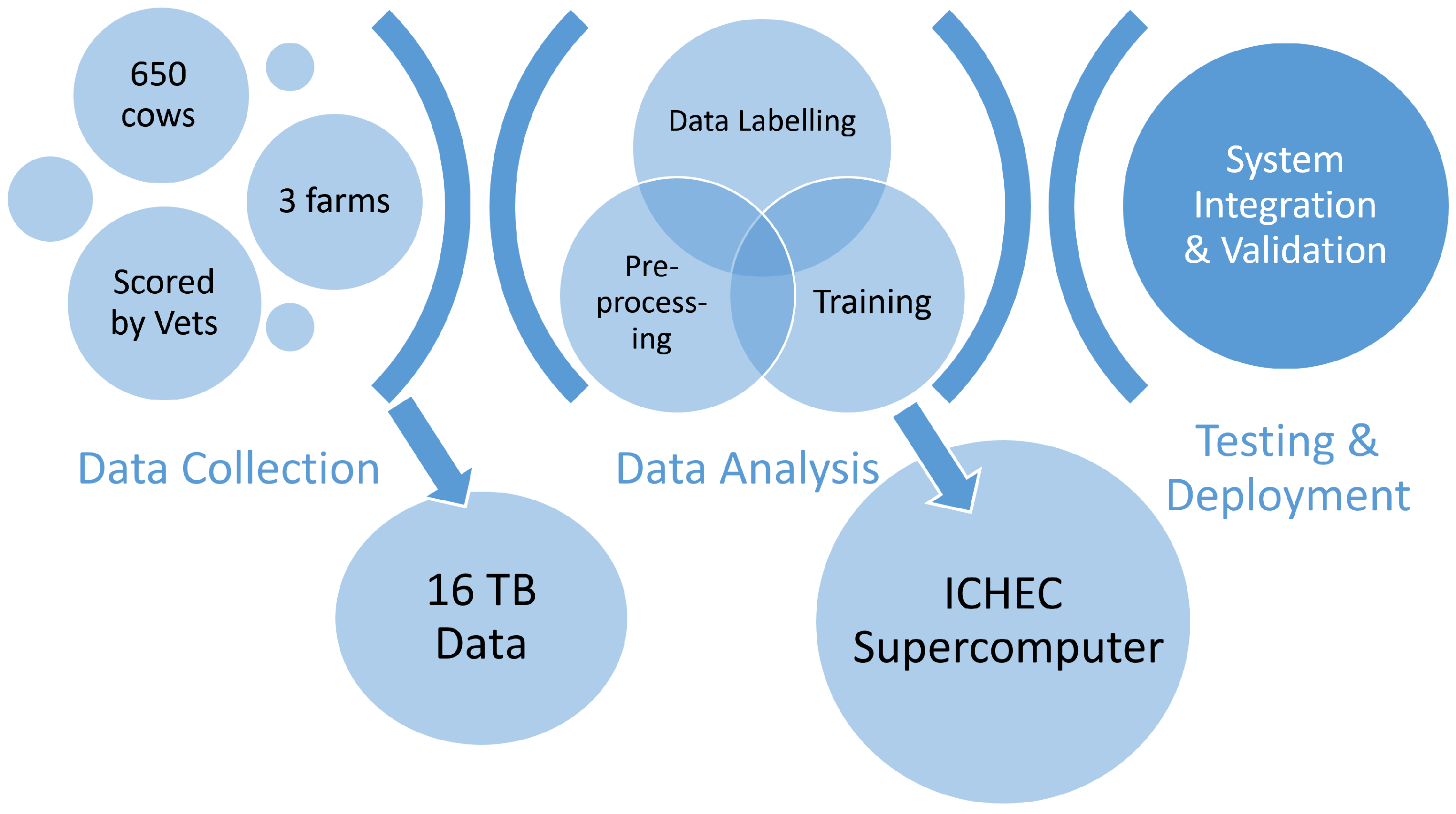
The latest research in Body Condition Scoring (BCS) estimation for Precision Livestock Farming (PLF) show a trend towards the use of 3D cameras and deep learning has improved the ability of these systems to deal with a greater variety of sensing scenarios through automatic feature extraction, improved accuracy and more reliable operation. This article will seek to advance the research in this area by analysing the challenges in using manual expert-provided scores as a ground truth reference and developing an Automatic Cattle Monitoring (ACM) system that addresses problems around the deployment, accuracy, sensitivity and maintenance of such a system. In examining the systems documented to date for automatic cattle monitoring, most techniques seem to be largely adaptions of Convolutional Neural Networks (CNNs). This prompted the development of a system to predict cow id and then BCS using Deep Learning(DL) paradigms. This prototype system highlighted a number of tools and techniques that proved useful in automatic cattle BCS monitoring, yielding a dataset with 2D and 3D camera data and expert-provided labels for BCS comprising 650 cows across three farms and demonstrated that state-of-the art level accuracies are achievable in both tasks using the latest 2D and 3D Deep Learning networks. More importantly, our trials highlighted problems with the reference data sources that are used for both tasks. The BCS scores provided by veterinarians featured inter-rater and even intra-rater reliability issues which impacts the agreement achievable by an automated system when transferring knowledge between farms.
The state of the art in automatic BCS estimation is reviewed in [4,5] and summarised in Table 1 under categories such as the size of the test dataset, the degree of automatization, the type of camera used and the accuracy of scores within 0.25 of manual BCS reference. Accuracies of 79% within 0.25 are achievable at scale with as high as 86% being achievable on some small datasets. Simultaneously the cost and complexity of the sensing equipment has come down (early 3D scanning required an array of expensive scanners). The main challenge that remains in the face of the adoption of these systems is the delivery of reliable repeatable results with enough resolution that the system can detect deviations in BCS for each individual animal. At present the fluctuations within the error margin of the state of the art and the potential for occasional false positive indications of extreme BCS due to sensing/dataset anomalies hinder the uptake of automated systems.
2.1. Deep Learning
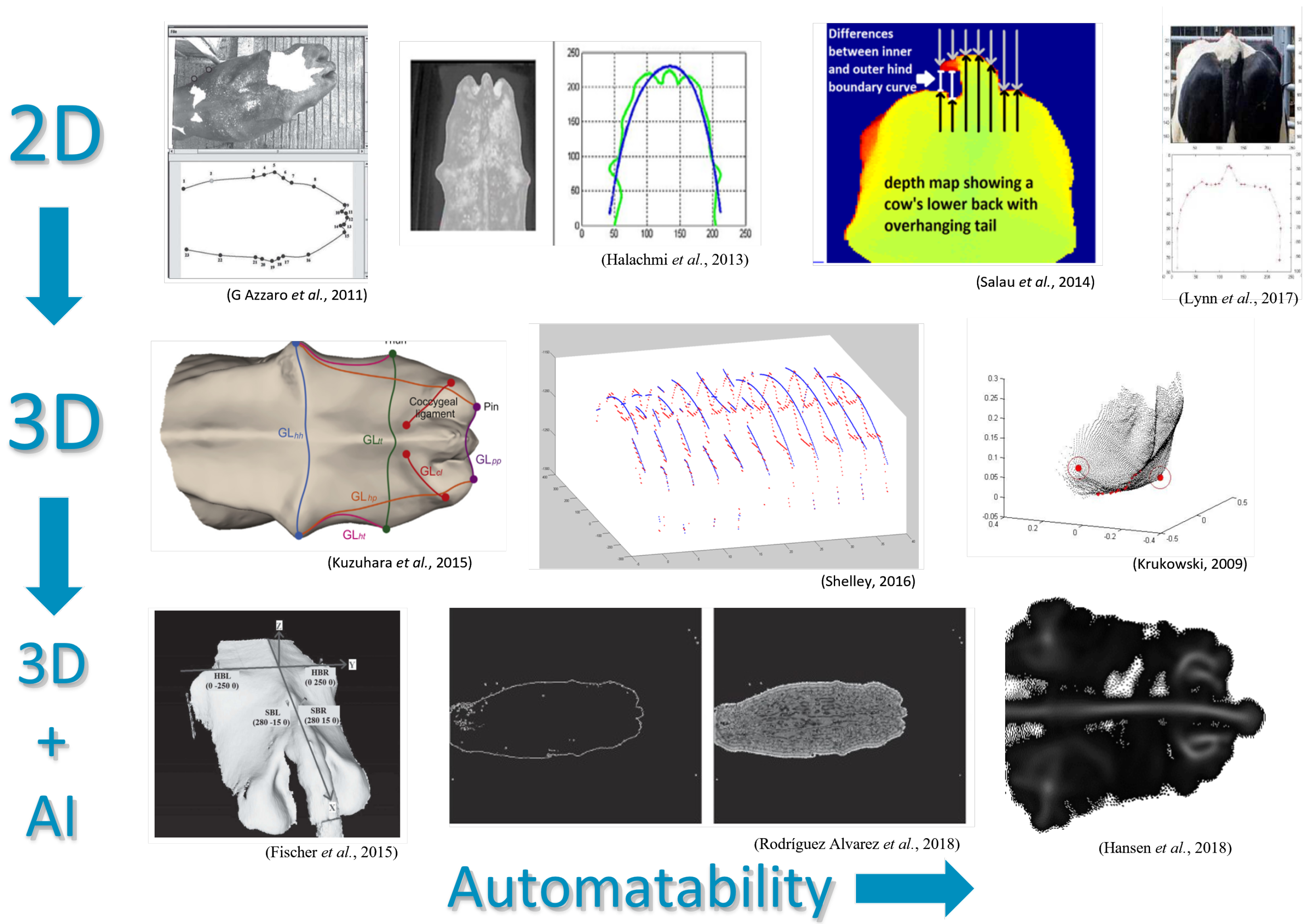
Automated BCS systems have advanced with the available technology as illustrated in Figure 1. The most prevalent trend identified is the uptake of 3D vision. With regards to what parts of the cow the vision system should capture, most implementations take a top-down view and are interested in features such as the curvature of the spine, hips and pins, while some take a side-on view and look at features such as leg swing, the curvature of the spine and the placement of the cow’s hoofs.
ToF cameras best fit such applications as they provide their own light source, they provide reliable measurements in real-time with the required precision (as proven by [18,19]) and they are available in IP69 rated enclosures. The precision and applicability of measurements gathered from a ToF camera (cameras being placed approximately 0.5m from the cow) were assessed by [20] where the heights of ischial tuberosities, i.e., the pins of the cow’s pelvis, were calculated from the 3D coordinates. Measurements taken with cattle standing still showed a standard error range from 2.4 to 4.0 mm for the heights of the ischial tuberosities. The accuracy decreases when the animal is moving to 14– 22.5 (+550%) mm, respectively, for each type of measurement. Therefore, the technology is practical for determining accurate measurements for assessing traits in cattle.
2.2. Deep Learning
A further trend has been the development of algorithms which make use of AI for improved accuracy and reliability. Many recent papers make use of a popular DL technique called Convolutional Neural Networks (CNNs) which are designed to automatically and adaptively learn spatial hierarchies of features. Such developments have been shown to beneficial in situations where the system may be deployed in a diverse range of conditions considering that physical traits can vary greatly depending on the stage of lactation and cattle breed and also that poor lighting and lens fouling are likely to occur in farmyard environments.
Manual feature definition is sometimes very difficult for high-level features—it is up to the CV engineer’s judgment and a long trial and error process to decide which features best describe different classes of objects. Poor model/feature definition, the introduction of unwanted bias from pre-processing steps and changing environments can lead to a lack of robustness. Machine learning rejects the traditional programming paradigm where problem analysis is replaced by a training framework where the system is fed a large number of training patterns (sets of inputs for which the desired outputs are known/discoverable) which it learns from to create a model which can be applied to new data at the inference stage. Machine learning can automatically learn complex mapping functions directly from data, eliminating the need for features to be manually defined [4].
Recently, there has been a big jump in our ability to recognise complex features thanks to a development called deep learning (DL), and more specifically, the neural network (NN) computing architecture, which emulates the theorised functioning of the human brain. The adjective “deep” is often assumed to mean that the architecture consists of many layers of computing cells, sometimes called “neurons”, that each perform a simple operation. The result of each computation being an activation signal that is passed through to the neurons in proceeding layers. Each neuron assigns a weight to each of its inputs and adds a bias value if necessary. By tuning these weights and biases, a model can be trained/learned to capture “deeper” local information and features through exploiting self-organisation and interaction between small units [4]. It is also for this reason that deep neural networks (DNNs) are often computed using GPUs, or similar hardware suited to matrix multiplication, and the availability of such computing resources is what has fuelled the recent activity and great strides in the predictive capability of artificial intelligence.
DL introduced the concept of end-to-end learning where the machine is just given a dataset of images which have been annotated with what classes of objects are present in each image. Thereby a DL model is ‘trained’ on the given data, where neural networks discover the underlying patterns in classes of images and automatically works out the most descriptive and salient features for each specific class of object. It has been well-established that DNNs perform far better than traditional algorithms, albeit with trade-offs with respect to computing requirements and training time, with the current state-of-the-art approaches in cattle monitoring employing this methodology [21].
2.3. 3D Deep Learning
Many of the state-of-the-art techniques in cow monitoring reviewed have used pre-processed depth images as input where the 3D spatial relationship between all points measured by the 3D camera is not captured [21,22]. Very few studies have exploited the potential of the point cloud data collected by 3D cameras, however, as the majority of algorithms use the depth image as input and those that have used point cloud data have only explored statistical techniques [13,23,24]. We propose that deep learning techniques which operate on the raw point cloud data, would yield better accuracy and reliability as it allows geometric pre-processing and noise reduction techniques to be applied and the shapes present in the point cloud would be invariant of camera pose, light amplitude and background light. As an emerging field, 3D CV has many open challenges including sensor fusion to improve the performance of range imaging systems, deformable 3D shape correspondence, generalization of deep learning models and dealing with dynamically changing shapes in 3D camera streams. The processing of 3D data also imposes greater memory requirements compared to as the convolutional kernel must convolve over 3 dimensions which results in an increase in computational complexity from to . Compared to 2D image processing, 3D CV is made even more difficult as the extra dimension introduces more uncertainties, such as from occlusions and varying cameras angles.
Geometric Deep Learning (GDL) deals with the extension of DL techniques to 3D data. 3D data can be represented as graphs, manifolds, meshes and point clouds depending on the application. As CNNs are the most effective DL architecture, many have adapted CNNs to take 3D data as their input and branded them 3D-CNNs. A diverse range of different methods have been proposed for 3D object recognition. Upon review, we note five types of architecture being developed: they are being view-based, voxel-based, convolution-based, point-based and graph-based [25]. One of the main difficulties in applying CNNs to 3D data is that the spatial relationship between features is lost due to the max-pooling layers. There have been many different adaptions to address these issues including projecting a 3D model into multiple 2D views, using CRFs to enforce geometric consistency of the output of 3D CNNs, and point-based methods with special transformations to ensure spatial awareness.
3. Materials and Methods
The creation of a dataset with corresponding data on animal activity/events for each cow recorded over a long term (multiple lactations) will allow variations over the lactation (as well as longer-term variations) to be tracked. The primary case study for the system is at points around the milking parlour, e.g., at the first bail after the entrance reader in the parlour. The system will be integrated with the milking parlour control system to correlate the information for each cow for each image. Once trained, the system should be deployable to any other location around the farm (for instance, cameras will also be installed above crushes/walkways/drafting crates) as such a system should provide real-time insights to allow decisions to be made at critical points in a pasture-based management system—when the cow is being fed concentrates, when the cow is being milked and when the cow is being drafted.
3.1. Camera Installation
A range of tests were carried out to determine if the available vision sensors were applicable to our desired application. To summarise, a range of criteria were evaluated, including accuracy, reliability of depth measurement across the field of view of the camera, long and short-range sensing applications, dynamic scene effects and remote deployment considerations. A low-power stereovision solution in the form of an Intel D435 camera [26] and an industrial Time-of-Flight (ToF) camera in the form of an IFM O3D313 [27] were tested. The ToF camera was chosen as it was found to be less sensitive to variations in lighting and provides more reliable depth measurements for fine-grained visual recognition tasks was chosen for the parlour vision system.
Through a literature review of the latest state-of-the-art technologies available in CV which may be applied in cattle monitoring [4], the most appropriate camera technologies and camera pose configurations were considered. This review was undertaken from both a hardware perspective and a software perspective. From a hardware perspective, the study found that state-of-the-art implementations use 3D cameras. With regards to what angles of the cow the vision system should capture, most implementations take a top-down view and are interested in features such as the curvature of the spine, hips and pins, while some take a side-on view and look at features such as leg swing, the curvature of the spine and the placement of the cow’s hoofs.
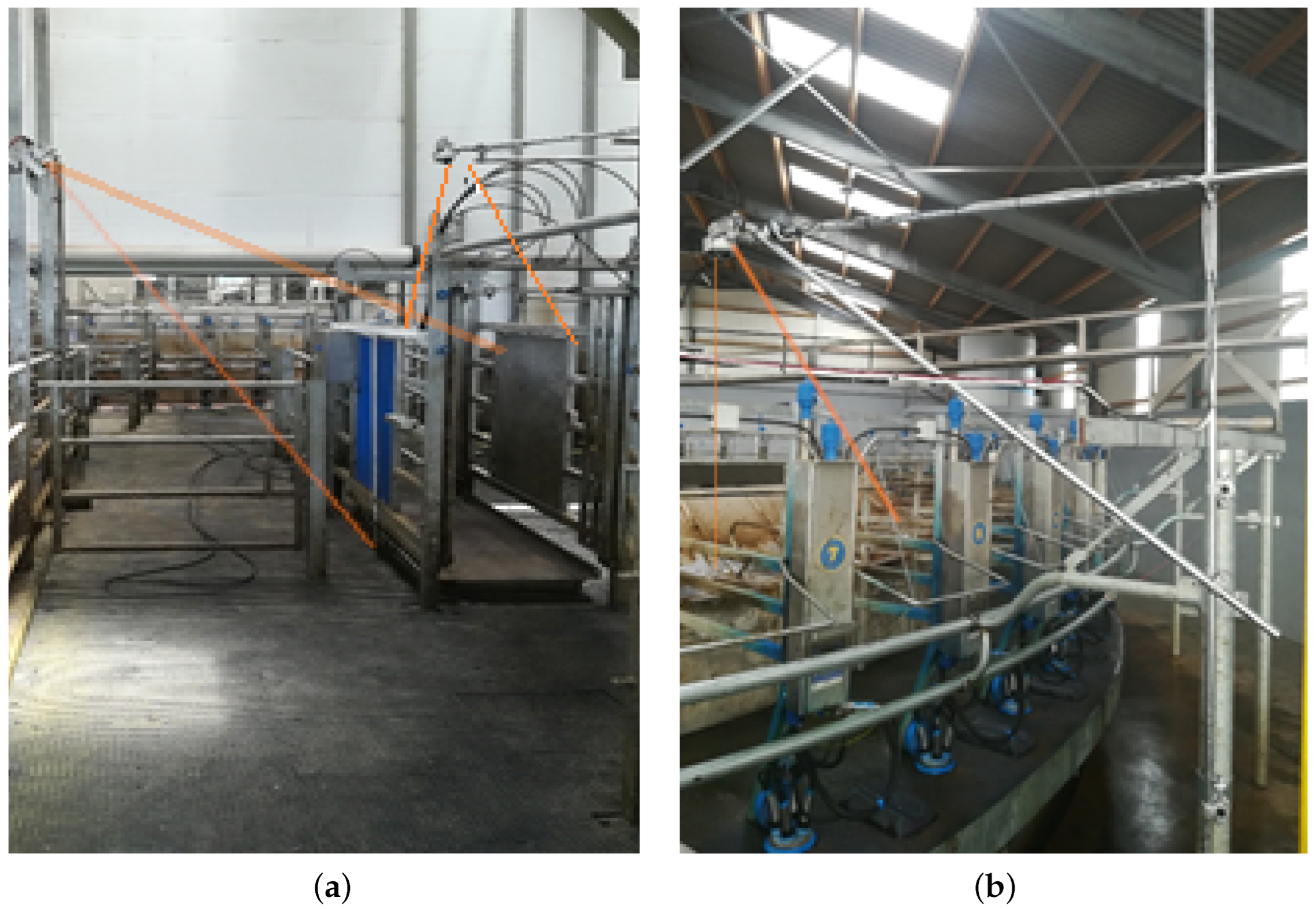
For our trials, we chose to view the animals from above (at locations shown in Figure 2). This places the camera high up and away from potential fouling and damage from animals or during the parlour wash routine. Both a ToF camera and a standard IP Camera were installed at each observation location. The view with a depth camera from above means that the curvature of the cow’s spine can be perceived which has been shown to be a useful indicator in BCS research. The IP camera provides a high resolution colour image which may aid the 3D camera if data fusion is used or prove to be a low cost alternative if trials demonstrate the analysis of the data can yield satisfactory results.
In our experiments we set out to devise methods which can learn from shape alone and are robust to rigid translation and rotation of the point cloud. Therefore ur experimental setup should contain such instances where the cow pose and environment changes. e.g., in the installation above the rotary parlour where the cow is not necessarily always at the centre of the frame, e.g., on the rotary as the cow revolves across the field of view (see Figure 3).
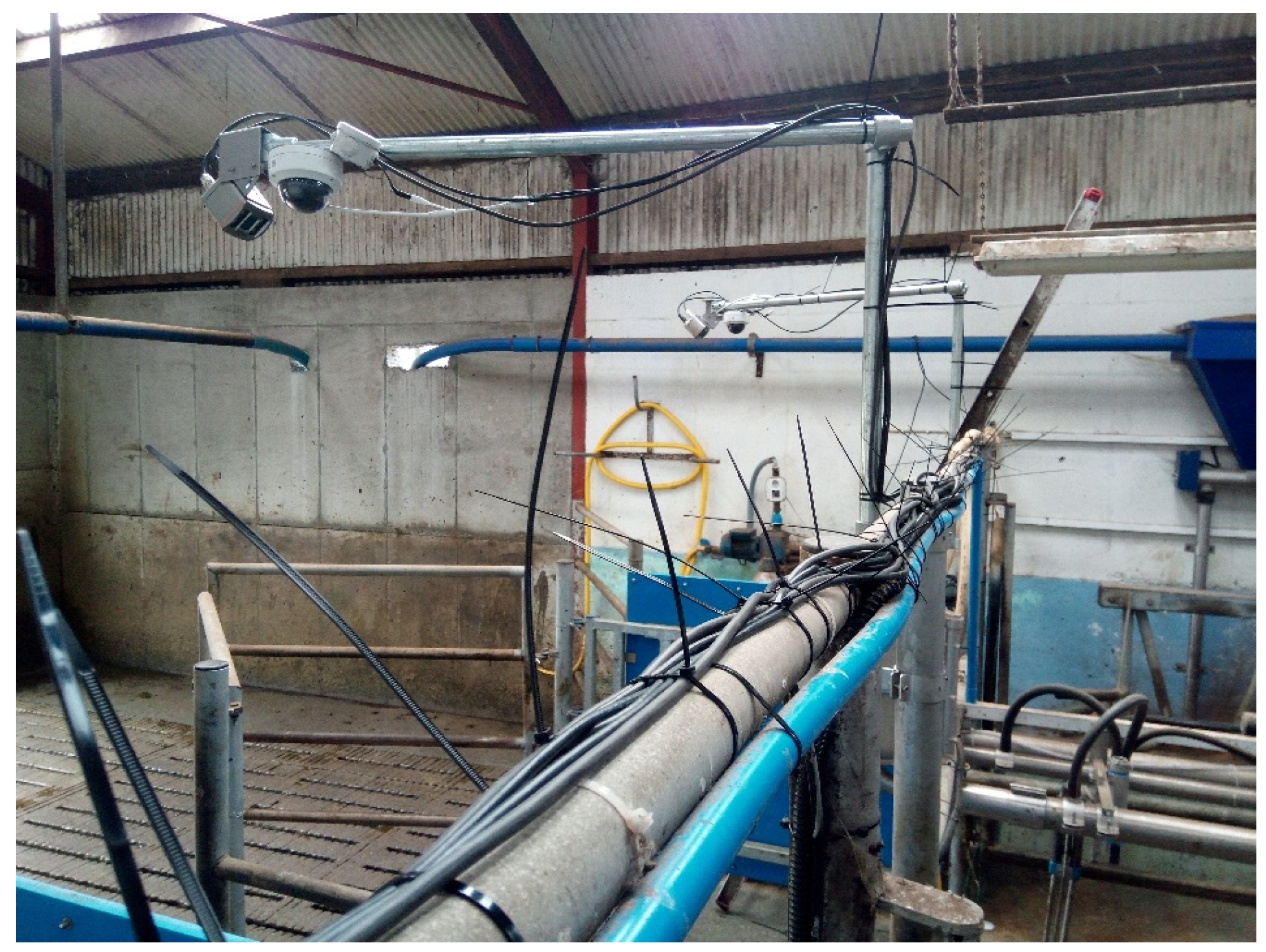
Moreover, the relative pose between camera and cow is not easily constrained either as it is sometimes necessary to point the camera at an angle to obtain a clear view unobstructed by the surrounding parlour infrastructure as shown in Figure 4. Additionally, cows can be moving quite quickly in some installation environments, such as at the parlour entrance, which makes accurate 3D measurements more challenging.
3.2. Data Acquisition
The camera is triggered when it is known the animal is passing underneath and the ID of the animal was logged through the use of an external RFID system. The recordings were stored in the file structure to enable access to the necessary information later during data analysis.
Vets provided regular BCS and Locomotion Scores at the Research Farm in UCD (University College Dublin) where the first camera trial took place which acted as a reference for learning to predict these animal Health indicators, while on 2 validation farms where subsequent trials took place, scores were provided thanks to the assistance of veterinarians at the Munster Technological University (MTU); Lea Krump and Gearoid Sayers. All herds had primarily Holstein Friesan breeding. Cows were assessed for BCS (a scale of 1 to 5 with increments of 0.25, where 1 is extremely thin and 5 is extremely fat) on a fortnightly basis. A summary of the data collected is provided in Figure 5.
The task is to automate the manual scoring of health attributes relating to the appearance of an animal’s shape. The reference scores which were taken as ground truth labels for the data were supplied by veterinarians and aligned with each animal in the data analysis phase through the matching of date and animal ID. The final label was then related to the corresponding veterinarians’ scores by look up table query based on animal ID and date. Taking the main research farm as reference, the acquisition system collected 70 sets of images/point clouds per cow per milking session for 200 cows. The data used for training was limited to very 10th image in which the cow was in frame which accrued to 1400 images per month and 11,200 images/point clouds over the 8 month collection period.
3.3. Image Processing
3.3.1. Keyframe Extraction
It is advantageous to be able to extract the keyframes when the cow is in the centre of the frame for both eliminating invalid frames from training data and also for limiting the number of frames over which a model is run at runtime. Due to challenging segmentation conditions (e.g., poor lighting and close proximity of animals to surrounding infrastructure), a wide range of keyframe extraction techniques were trialled and documented in the following paragraphs.
Depth-Based Foreground Extraction
The objective here was to detect cow presence using the segmented images using the watershed method [28] which could allow models to be trained with fewer data as non-relevant variations in the surrounding background would be removed. However, this work yielded unreliable results such as cows being segmented into multiple parts or not at all as shown in Figure 6. This may have been due to poor repeatability of the watershed algorithm in separating the cow from the background.
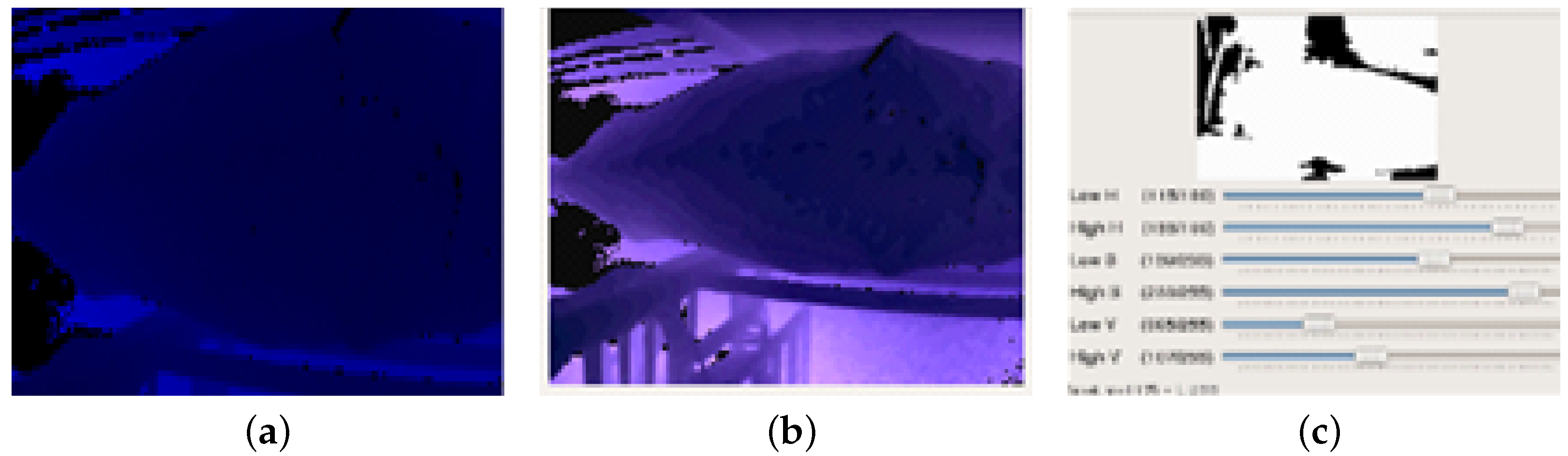
Colour Thresholding
The animals’ size and posture can vary significantly, i.e., as they walk and move their head as they pass through the cattle crush/milking parlour. This was found to be problematic when applying Colour space pre-processing (transformation to LAB and then HSV colour spaces) and binary amplitude thresholding to segment the animal from the image. The required tolerance to accommodate the variation in cattle shapes was found to be too great compared to the proximity of the cattle to the surrounding railings to successfully segment the cow (see Figure 7).
Difference Histogram
The absolute histogram difference-based method was found to be effective in finding images where the animal is moving, i.e., by setting a threshold on the minimum difference between the histograms of two consecutive image frames, the repeated images were removed and the frames containing animal posture and motion information are extracted. However, the method was not very useful in determining when a cow was fully in-frame and also in the given application we also want to run the analysis when the cow is fully in-frame and also static (thereby increasing the accumulated confidence in our prediction over several frames).
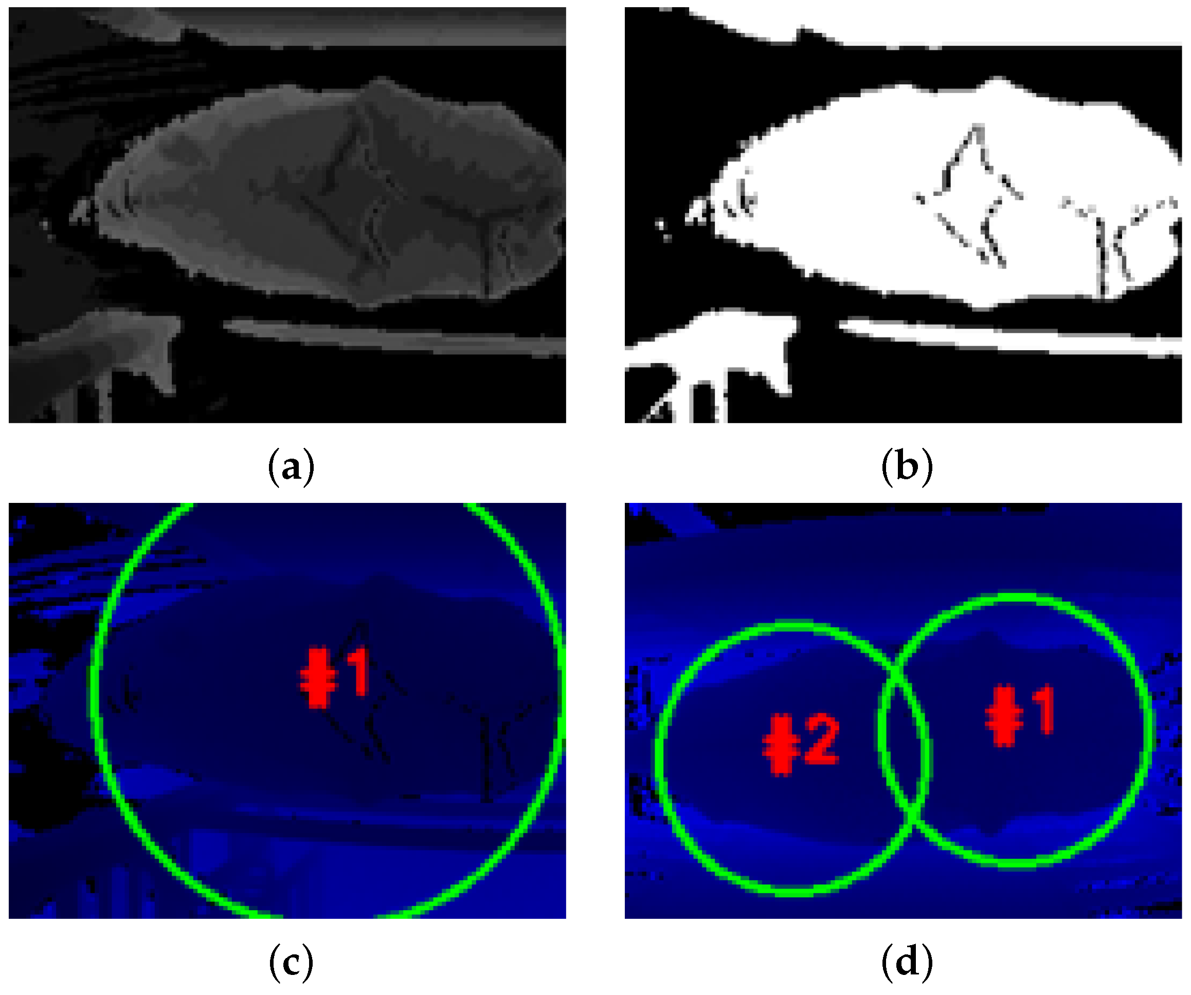
Depth Measurement at Image Keypoints
In some instances, animal flow is unimpeded, and animals can often follow each other closely which makes it difficult to identify the gap between animals in order to separate the recordings for each animal. It was found to be more effective and more efficient to simply query the pixel value at 5 distinct locations in the depth image where it was known that the area would be occupied/unoccupied, respectively, at the instant the animal would be in the right place. This method consisted of a simple program that queried the depth at 5 co-ordinates which in a keyframe would be located as follows: just in front of the cow, 3 points zig-zagged along the cows back and just behind the cow. If the depth for each keypoint was between certain thresholds for each respective keypoint (i.e., if the points before and after the cow were vacant and the 3 points in the middle were occupied by a cow), then the keyframes when the cow was in the optimum location for all features to be visible to the camera could be reliably detected. This technique was found to be the most satisfactory of the keyframe detection techniques presented in this section as it could be easily configured for new installation scenarios (albeit manually) to be triggered according to the desired cow profile/pose for BCS estimation to take place.
Normal Map Calculation
For the BCS application, it was found that it was useful to extract the curvature information of the cow’s topology by calculating the normal (the direction of the line perpendicular to the tangent to the surface) for each point. The normal map for an image may be calculated from two vectors calculated from neighbour pixels by merging Holzer et al’s method [29] and Equation (1).
where: is the Normal vector at a point , is a vertex map that corresponds to a camera coordinate, and the equation describes how the normal vectors are obtained by calculating a cross product of two vectors from neighbour points.
Initial results were unsuccessful in representing the gradient in height along the cow’s back because of noise in the depth image. Upon applying a bilateral filter to the depth images before the normal map estimation, the result was improved to what can be seen in Figure 8a.
The method was subsequently performed on images with the animal segmented as can be seen in Figure 8b. However, the models subsequently trained on the normal map calculated for the entire scene yielded the better results so that method was used ultimately.
3.3.2. Image Classification
In line with the latest state of the art, deep learning processes were implemented in order to yield models to predict Cow ID and BCS. With the rise of deep learning in the last number of years, plenty of frameworks and libraries that can be used for deep learning have been developed for open source use. This thesis has looked at a number of frameworks to test the various libraries/programming interfaces available, e.g., Keras [30], Pytorch [31] and Matlab [32]. A framework called TensorFlow [33] was used for these trials as it has the most flexibility and community support [34]. For training deep CNNs on the dataset of images collected was performed as detailed in Section 3.2 on data acquisition. The ‘depth Measurement at image keypoints’ method was implemented to ensure only images where a cow is in frame were used. Since the image acquisition system acquires 20–60 images per sighting of each cow, every 10th frame was taken to limit the amount of repeat data.
The entire scene captured by the camera was taken as input, i.e., no segmentation was applied. Images from both types of camera (2D and 3D) were trialled.
For the 3D camera data, the 3 image outputs from the IFM O3D313 camera were overlaid into a composite image as described in to satisfy the 3 channel format of the input to most available deep learning-based classifiers (i.e., the r, g and b channels typical in colour images were filled with the amplitude, depth and confidence streams from the 3D camera). Some preprocessing was applied to adapt the image to the format expected by pre-defined models (i.e., image resizing) and experiment with measures to highlight the curvature of the cows’ backs (i.e., normal map generation).
The data was labelled according to the file structure, i.e., for the cow identification task the cow ID is contained within the directory name was used as the target label, while for the BCS task, the label was assigned according to a look up function of the nearest BCS. A wide range of different types of models available in the TensorFlow object detection API were trained on the collected labelled data. As the models downloaded to use as initial checkpoints were initialised on general purpose datasets (e.g., ImageNet or MS COCO) the training procedure was a means of transfer learning, i.e., re-adjusting the weights and biases of the checkpoint network so that the output classes are reassigned to the set of cow ID/BCS classes defined in the dataset. Transfer Learning was found to work on new classes as that it turns out the kind of information needed to distinguish between all the 1000 classes in ImageNet is often also useful to distinguish between new kinds of objects.
Object Detection models where a bounding box is defined around each cow were used to focus the input data to just the information relevant to the cow per annotated image, i.e., removing irrelevant information about the scene in the background. The TensorFlow Object Detection API was implemented for BCS classification.
In this experimentation, we used the MobileNet-SSDV2, Inception-SSD and we trained the models using depth images, composite images and normal-map images to compare the results images from [15]. We resized the images to 224 by 224 resolution. No other pre-processing was done. We trained the models on a laptop equipped with a NVIDIA GTX 1060 GPU with a 6 GB memory. We set the batch size equal to 24 and ran the training for 25,000 training steps.
To maximise the classification accuracy, the accumulated confidence of each prediction for subsequent frames of every cow sighting. This method is useful in the scenario where the top-n predictions are of similar confidence. A high confidence filter was appended to the network architecture in Figure 9 where the sum of the confidence score for predictions that appeared most often with high confidence (the top-5 predictions per frame over 45 frames or 3 s) was used as an indicator to yield more consistent predictions. The results of these trials are shown in Table 2.
3.4. Point Cloud Processing
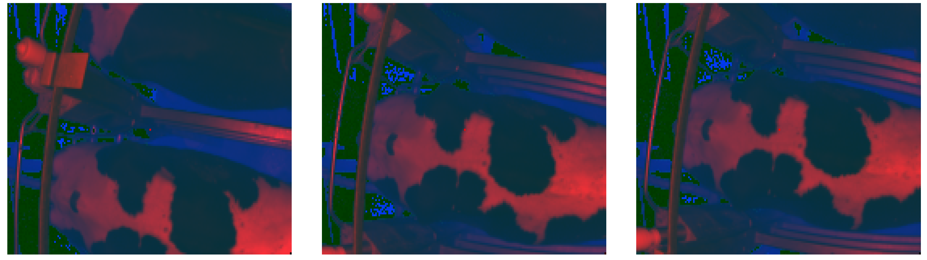
Issues arising from a change in farm/pose/environment were found to be detrimental to model performance (e.g. cameras mounted in a different location and orientation result in inconsistent presentation of the data as illustrated in Figure 10) and tightly constraining the camera installation configuration is not an feasible. Hence, the proceeding section will investigate methods which operate on the more native representation of the 3D data going through the steps of keyframe extraction, data pre-processing/transformation, neural network training and the refinement of inference results and compare them with their 2D counterparts to answer the question of whether it is better stay in the well-established 2D domain or try and exploit the extra relational information in raw point cloud data.
3.4.1. Dataset Preparation
Keyframe Extraction
Applying some segmentation techniques to verify the cow is in the correct position using the point query method in the depth image and so filter the training data was found to improve the quality of the proceeding inference results. The training data was limited to only days within 2 days of when cows are scored to omit any deviation cows may exhibit in the intermediary periods between score dates. Different pre-processing steps for the point cloud data were also trialled using Point Cloud Library [36] including:
Primitive Shape Matching Segmentation
Model-fitting methods for point cloud segmentation, such as Hough Transforms [37] and Random Sample Consensus (RANSAC) [38,39], may be used to fit primitive shapes such as planes, cylinders and spheres to point cloud data. The points that conform to the mathematical representation of the primitive shape are labelled as one segment. RANSAC is fast and efficient, less sensitive to noise and outliers, maintains topological consistency and avoids over- and under-segmentation. However, these methods are highly dependent on the subject matching a known shape which means the method falls short for complex shapes or fully automated implementations and was found not to be applicable where the subjects are animals as a combinations of dimensions and tolerances for planes/cylinders/cones (see Figure 11) could not be found to consistently segment the cow/background points.
Region Growing Point Cloud Segmentation
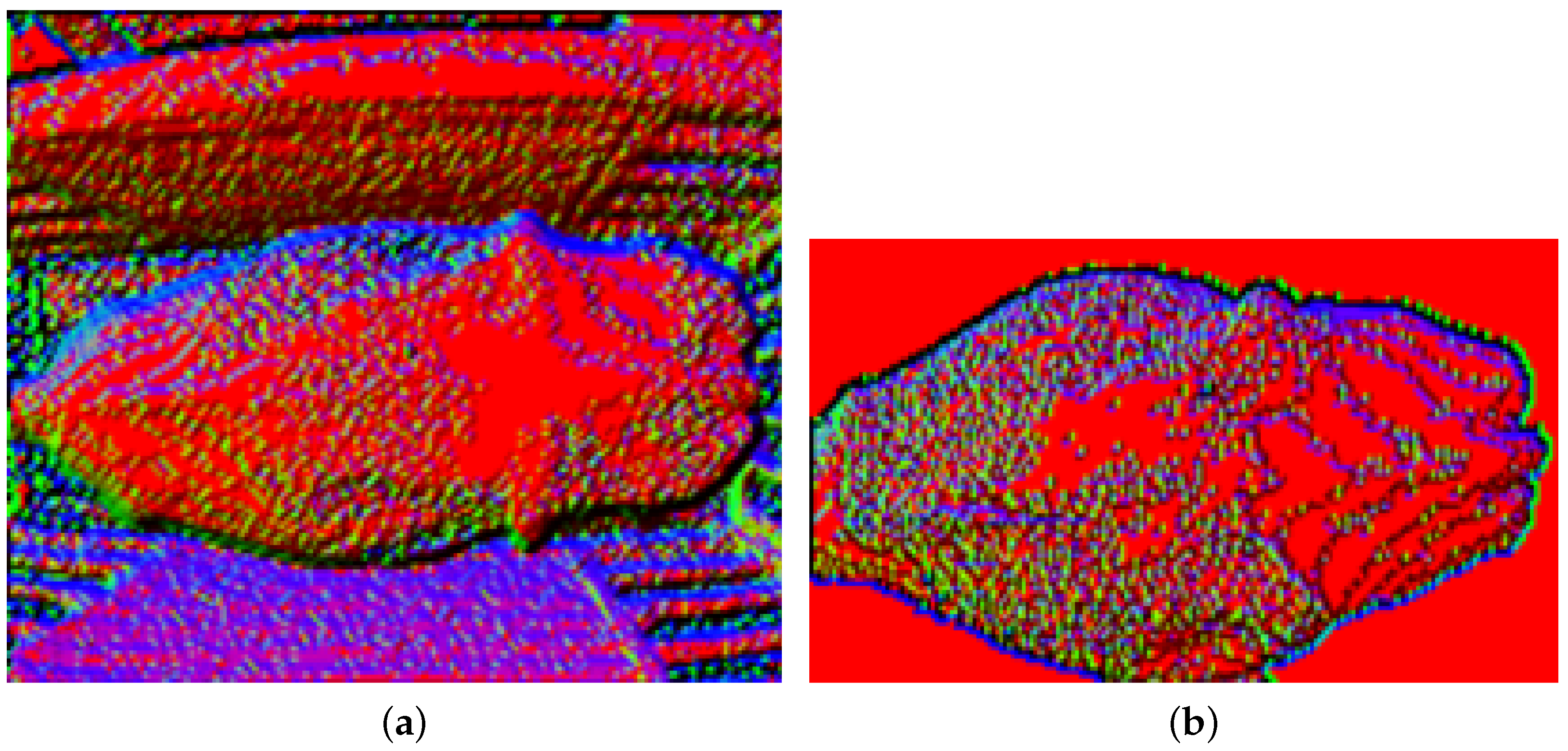
Region growing segmentation [40] is a bottom-up approach that starts from some seed points and grows the segments based on given similarity criteria. The method is more robust to noise through the use of global information but is sensitive to the location of initial seed regions and inaccurate estimations of the normal and curvatures of points near region boundaries. The similarity criteria used in the trial of this method was to group points which are spatially close and share similar normal vectors. The method was found to work quite well (see Figure 12) once tuned to the characteristic point density and curvature of the data captured by the camera for the scenes in question.
Point Cloud Annotation
Dataset creation and annotation is a huge bottleneck in 3D DL, particularly in 3D segmentation tasks where every point in 3D space must be labelled accurately. Ref. [41] include a review of some creative ways of improving the data annotation process in terms of efficiency, accuracy and automatability. Several annotation tools exist which have improved the user interface for point cloud annotation, for our dataset, we used an adaption of [42].
In our annotation automation schemes we delegate as much of the work as possible to the machine while still giving the user insight and control over the process. We followed such a scheme to segment the cow from the background in the parlour vision system dataset. Traditional region growing segmentation was used to annotate point clouds over narrow spectrums of circumstances. That is a segmentation strategy was defined that works for a given set of conditions, take the segmentation results and combine them with the results of the same process adjusted to a different set of conditions. Doing this in an iterative manner allows complicated to be annotated many scenes at a time offering a drastic speed-up compared to annotating point clouds one scene at a time manually.
3.4.2. Data Pre-Processing/Transformation/Point Cloud Downsampling
Following segmentation, it is necessary to downsample the isolated cloud of the object to be classified if it is to be inputted into a neural network. There are several useful filtering and downsampling techniques which may be used to ensure the quality of data being fed to the network. Rather than listing them all, let us demonstrate how the point clouds were filtered in our implementation.
Firstly, the point cloud was represented as a voxel grid so that statistical outlier removal by K-means clustering [43] could be performed followed by radius outlier removal. The combination of these two techniques allowed both point outliers due to noise and groups of points due to sensing artefacts and/or incomplete segmentation of the background in the previous step to be removed effectively.
It is necessary to input a fixed number of either 512/1024/2048/4096 points to many of the neural networks trailed for our application. Therefore, many subsampling methods which allow for the desired number of remaining to be set were implemented and compared. The point clouds were reduced from approx. 8000 points to 4096 points using random sampling and normal-space sampling. As is shown in Figure 13, density-based sampling such as normal-space sampling or farthest point sampling removes more points in the flat parts where there is not much detail while keeping the important parts near the tight curves.
3.4.3. Point Cloud Classification
The latest state-of-the-art models for each of the categories of data representation were reproduced using the open-source repositories included in the respective references and adapted where necessary to run on our custom data. These included:
These networks were implemented in combination with various combinations of the keyframe extraction and data pre-processing steps as shown in Figure 14. Several training iterations were performed to tune the parameters to our data (e.g., the l1-l4 radii which define the range of sizes of feature you want to look at). A script was also written to sample the point cloud into box sections randomly and feed these point sets as the training input. This worked well as the networks seemed to train better with point numbers <8192 because it allows larger batch sizes and doing it this way avoids downsampling the point cloud too much.
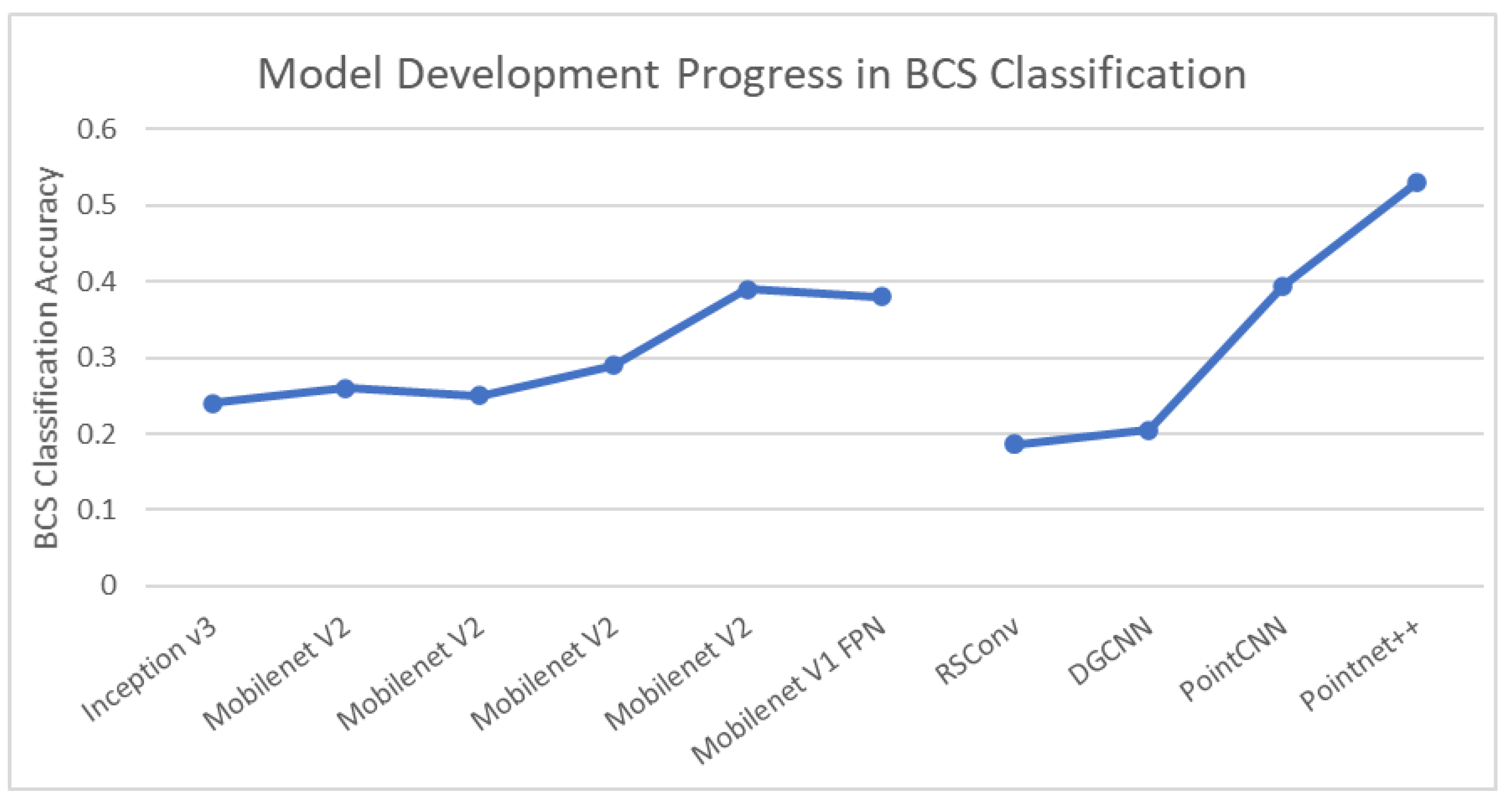
These networks were implemented in combination with various combinations of the keyframe extraction and data pre-processing steps discussed previously as detailed in Table 3. With regards to 3D augmentation, rotation and translation and jitter, i.e., the introduction of random perturbations to each point in the point cloud, are standard techniques. These techniques were found to be effective when selectively applied to the minority classes in our implementation of PointCNN which improved accuracy substantially compared to the other 3D model results from an accuracy of 39.4% of the next best model PointCNN to an accuracy of 53.0% (Table 3). This result was also facilitated by mitigating the class imbalance present in the data by using selective data augmentation (applying random rotations and jitter only to the classes for which few data are available) and by adjusting the weights for each class according to their representation in the training set.
The gradients of state-of-the-art networks such as PointNet and PointCNN were tuned to the easy-classified samples present in the 3D point cloud benchmark datasets such as ModelNet or ShapeNet, making hyperparameter initialization very challenging when it comes to applying these networks to custom datasets. Table 3 shows the results of the experimentation which was carried out. Recall the max classification accuracy achievable using the 2D methods discussed in the previous section was 0.39.
Hyperparameters proved to be determinant in the training process. In the early stages of the experiments, the size of the mini-batches fed to the network was bigger and the highest accuracy achieved was 0.394 accuracy, but this value reduced in later stages. Data pre-processing and checking is fundamental. Varying the test, train and validation sets after the data was clear of imbalances had minimum impact onto the model.
4. Results
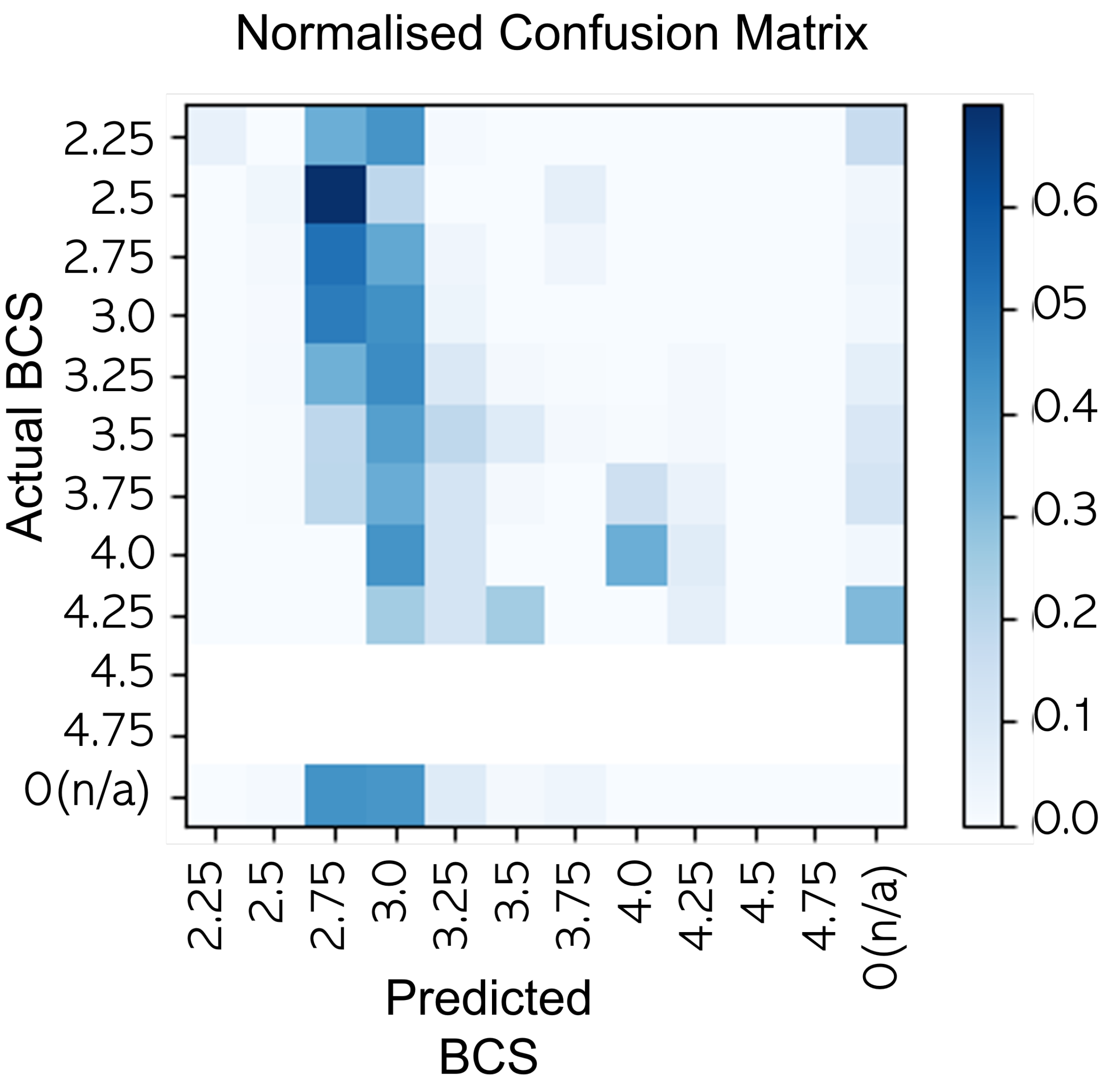
The scarcity of samples in some of the object categories leads to problems during training where the validation loss increased as training progressed. 57% of the cows in the dataset had a BCS of 2.75 (the majority class) which lead to the models being more biased to score 2.75. BCSs at the extremes of the chart (<2.0 and greater than 3.5) were recorded live in less than 22% of the scores, whereas the same 2 to 4 scores (2.75 to 3.25) accounted for up to 78% of the scores with 57% of the cows being scored 2.75.
This deviation from normal distribution did not sufficiently expose the model to these extreme BCS points during initial testing. To give an idea of the distribution of correct predictions, confusion matrices were calculated and are shown in Figure 15. This class imbalance within the dataset prompted the need for data augmentation techniques to be applied to the under-represented classes so they could be over-sampled. There are other options such as under-sampling the majority classes. An alternative to dataset management is to use a Weighted Loss function such as the Focal Loss function in Mobilenet V1 FPN which yielded the best accuracy in Table 2), yielding an accuracy of 38%, 90% within 0.25 and 95% within 0.5.
This high-confidence aggregation approach was found to work well when the cow is stationary for the observation period and was found to be less effective for the Rotary images where the platform is constantly moving and would not be applicable in cases where cows are not stopped at the drafting crate.
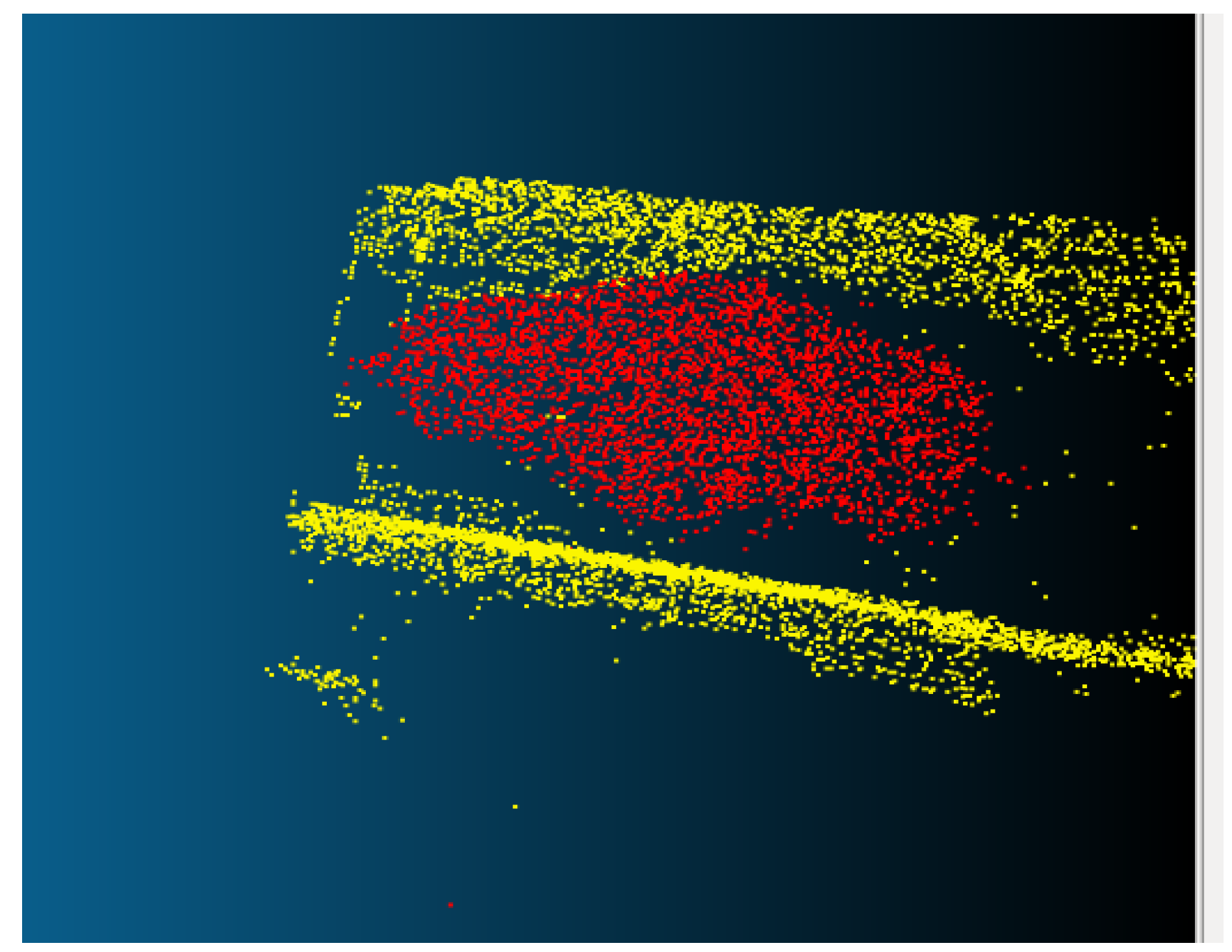
Of the 3D DL models tested in Table 3, PointNet was proven to best learn the relevant features of the data. To achieve this result, Region-of-Interest segmentation + minor Normal-Space Subsampling and block merging techniques previously discussed were combined. The results after this step were 98% semantic segmentation accuracy in cow segmentation (extracting the cow from the background and for BCS the semantic segmentation accuracy was 53% (which was better than previous methods described in this paper as charted in Figure 16). Visualisations generated of the semantic segmentation results for BCS classification show how different areas are attributed to different BCS scores. As can be seen in Figure 17 the BCS predicted is consistent across the cow and the cow is accurately segmented from the background.
Further comparisons in this paper will compare the best preforming of the 2D and 3D methodologies trialled (i.e. Mobilenet V2 with normal map preprocessing from Table 2 and Poinet++ with region growing and normal space subsampling from Table 3), hereafter referred to as Algorithm 1 and Algorithm 2 respectively.
5. Repeatability Evaluation for the Scoring Tasks
Human scoring is identified as the gold standard in BCS. This is problematic as it is a subjective assessment which is prone to poor inter-observer and intra-observer reliability. Therefore, the repeatability of estimation of observers needs to be evaluated if the system designed to replace this gold standard is to be compared fairly.
A metric which is often used to quantify repeatability is Cohen’s coefficient, a traditional measure originally designed as a measure of agreement between two judges, based on the Accuracy but corrected for chance agreement. It uses a scale of poor (<0), slight (0.01–0.20), fair (0.21–0.40), moderate (0.41–0.61) substantial (0.61–0.80), or almost perfect (0.81–1.00). The definition of is
where is the relative observed agreement among raters, and is the hypothetical probability of chance agreement, using the observed data to calculate the probabilities of each observer randomly seeing each category. If the raters are in complete agreement then . If there is no agreement among the raters other than what would be expected by chance (as given by ), . It is possible for the statistic to be negative, which can occur by chance if there is no relationship between the ratings of the two raters, or it may reflect a real tendency of the raters to give differing ratings.
Kristensen et al. (2006) conducted a study to estimate the agreement on exact scores among practising dairy veterinarians attending a teaching workshop on BCS and the ranged from very poor (0.17) to good (0.78), with a moderate average (0.50). These levels of agreement in exact scores between assessors were similar to our findings. Consequently, comparisons between assessors of herd BCS are not warranted unless repeatability assessments have been performed and a need exists to provide more estimates of the repeatability of BCS among consultants working in the field. Allowing an agreement within 0.5 points seems to be necessary to achieve excellent agreement (Kw > 0.80) between many assessors for assessment in uncontrolled situations and to allow comparison of herds [48].
From analysis of the manual scores for the first day of scoring on the verification trial, the vets had an inter-rater reliability value of 0.268–0.296 and each of the vets had intra-rater reliability of 0.449 and 0.27, respectively, for the 205 cows scored.
can be inadequate when an imbalance distribution of classes is involved, i.e., the marginal probability of one class is much more (or less) greater than the others. For example, BCS is typically normally distributed about BCS 2.75–BCS 3.0, so the reliability calculation should ideally take into account the percentage distribution of each score. Krippendorff’s , a statistic with the same structure as but that differs from it in the definition of in Equation (2) according to the method by [49]. The advantage of this approach is that it supports categorical, ordinal, interval, and ratio type data and also handles missing data [49]. The Krippendorff’s calculation used the percentage distribution figures for the BCS scores established for Validation farm 1.
As for Cohen’s kappa, Krippendorff’s alpha is defined via the formula in (2). Except now, for and the relative observed agreement among raters uses a weighted agreement table where agreements are weighted inversely to statistical probability. Hence agreements that are more likely are down-weighted, yielding a more conservative reliability score compared to Cohen’s .
The model (trained on two farms) was run on the test set omitted from training (basically any cows whose number ended in 0 or 1) on the day they were scored for both morning and evening. The results are in Figure 18 and Figure 19.
The kappa values for this test set of 15 cows were as follows:
- The 4 reference BCS sores had a Krippendorff’s of 0.51 (inter-rater reliability)
- Each vet had a Krippendorff’s of 0.39 and 0.79, respectively, (intra-rater reliability)
- The Inferences morning and evening had a Krippendorff’s of 0.70 (machine reliability)
Below is a correlation matrix between the observers and the machine on the day of scoring on a test set of 14 cows which the model had not seen during training. Rater 1a and 1b denote the scores given by the first vet on their first and second sighting of the animal. Rater 2a and 2b denote the same for the second vet. Algorithm 1 is the results of the best 2D model for the morning milking and Algorithm 1b is for the evening milking. Likewise, Algorithm 2a and 2b are the results of the best 3D model for the morning and evening milking. The 4 values in each cell correspond to Krippendorff’s coefficient, accuracy, accuracy within 0.25 and accuracy within 0.5 in that order. As can be seen, the machine is better than the inter-rater results, more repeatable and more accurate than rater 2 and more accurate but not as repeatable as rater 1. However, in the context of on-farm assessment, if the sole goal of BCS is to only detect cows with extreme conditions (e.g., identifying too thin cows as a sign of illness or nutrition deficiency and identifying over-conditioned cows which may be more prone to disease at calving), it may be arguable whether such fine level of precision of BCS is needed. As those extreme cows are rare in the population, it may be sufficient for the system to be able to differentiate extreme from normal-condition cows to allow benchmarking farms on cow welfare level (i.e., categorizing farms in percentages of too thin, too fat and in ideal condition). On the other hand, from a management perspective, it may be important to distinguish these extreme scores to monitor changes at the cow level.
The test was repeated for the second validation farm also. Below is a correlation matrix between the observers and the machine on the day of scoring. This was computed on recordings collected that morning. 122 cows were scored by the vets that day of which 110 were recorded machine-scored at least once and 73 were recorded and machine-scored twice (some cows are missed due to not read by RFID, not detected to have come in-frame by the algorithm or no score with high enough confidence produced).
The inter-rater and intra-rater repeatability metrics were again compared with the CNN algorithm developed in Section 3.3. This test compares of the robustness of 2D vs. 3D deep learning approaches. In this comparison, we denote the Mobilenet V2 model on normal map in Table 2 which gave the best results at the research farm and validation farm as Algorithm 1.
The repeatability was evaluated for Algorithm 1 in Table 4, where Algorithm 1a and 1b refer to the algorithms first and second look at the cow when she passed through the parlour the morning and evening of the same day. Poor agreement results (negative Krippendorff’s values (−0.135 to −0.149) means disagreement) between the vets and Algorithm 1 are observed. This is suspected to be due to change in camera installation orientation to what it was trained on in the UCD research farm, i.e., it is further back from the cow which was necessary due to bars obstructing the view at the point the RFID is triggered. Furthermore, cows are moving very fast and only one or two frames are available per sighting. Due to this suspicion the latest 3D CNN (PointNet model in Table 3) were also tested and is denoted as Algorithm 2 in Table 4.
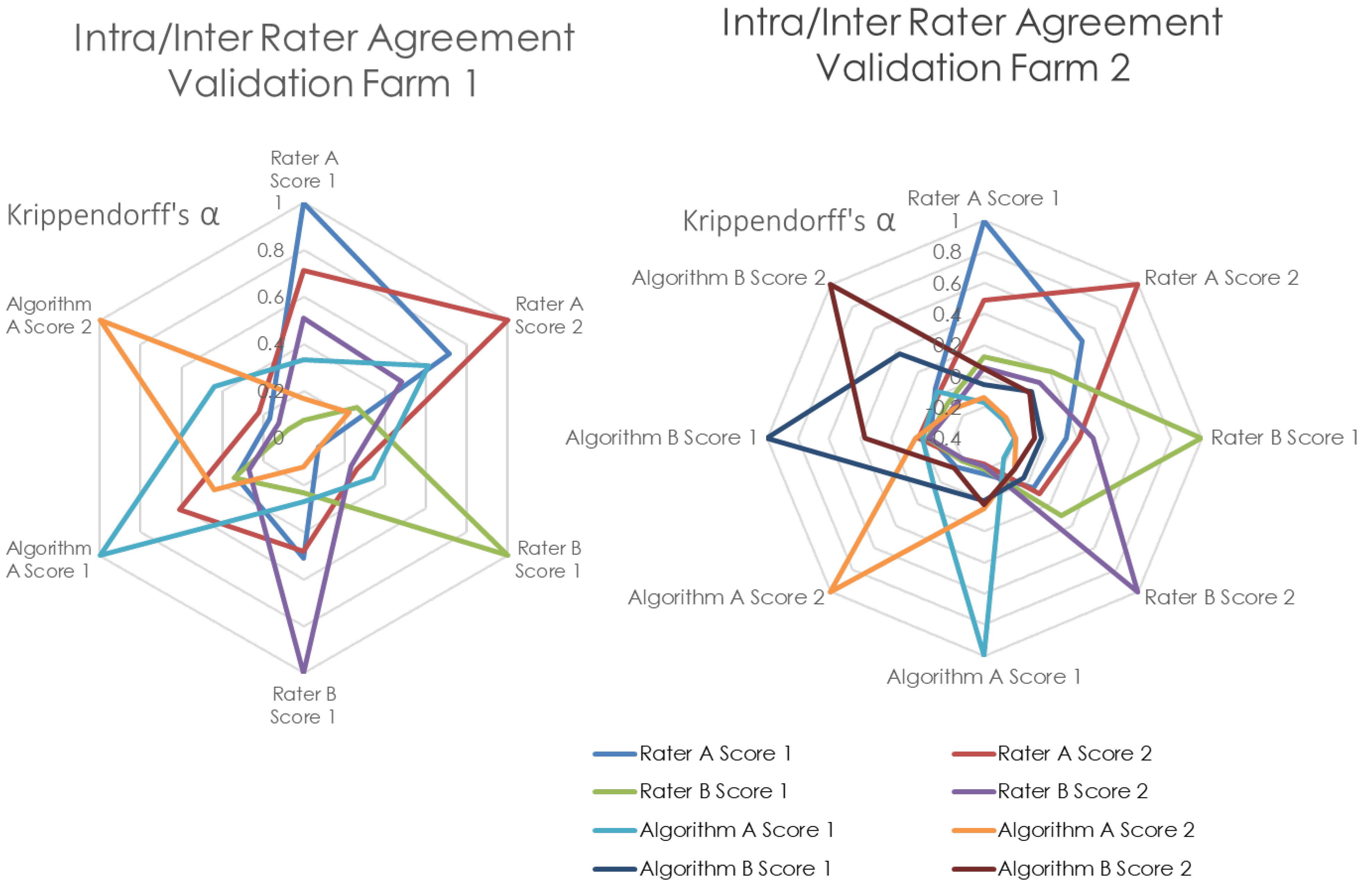
As can be seen, the intra-rater reliability for the machine achieved slightly better agreement with itself (Krippendorff’s of 0.372) compared to the average intra-rater reliability for the the vets (Krippendorff’s of 0.289). However, the model is still not in agreement with the vets with a Krippendorff’s of −0.077. All inter/intra rater reliabilities of the best 2D and 3D DL models are represented in a radar graph in Figure 20.
6. Conclusions
The results from deploying deep learning models developed for automatic cow monitoring, specifically in the task of BCS estimation in a research farm and two more validation farms have many interesting findings. This investigation gave insights into the question; given a real-world classification problem to be tackled with 3D depth-sensing cameras, whether it is more advantageous to use the depth image and apply 2D CNNs or to use the point cloud data and apply 3D Neural Networks? It was found that, while 2D approaches can be advantageous in leveraging a wider breadth of datasets and pre-trained models, it is more advantageous to use 3D methodologies which are more robust to noise and inconsistent camera/subject pose for deployment in unregulated environments. Overall, techniques towards minimising class imbalance and extracting curvature features (normal map calculation) were found to be effective in improving the performance of the models. The respective best 2D and 3D methodology achieved BCS estimation accuracies of 54.6 and 77.04% within 0.25) when deployed to a different farm which indicates that the 3D method was more robust.
However, deploying the classification algorithms to several farms and comparing the agreement between vets scores and the scores generated by the model has indicated that while the model can achieve the same repeatability as expert observers (a Krippendorff’s coefficient of 0.289), it does not agree well with the observers for that herd having been trained on a different herd (a Krippendorff’s coefficient of −0.077). This article presents strong evidence that there is an issue with the reliability of manual scoring which is problematic when trying to train a machine learning model with human-provided ground truth across farms. This means that trying to emulate a single scorer on one farm may not necessarily yield enough sensitivity to be able to alert the farmers to changes in BCS reliably and quickly enough for effective and prompt correction. We intend to tackle this problem in an upcoming paper.
Author Contributions
Conceptualization, N.O.; methodology, N.O., L.K. (Lenka Krpalkova), G.S. and L.K. (Lea Krump); software, N.O.; data curation, N.O. and L.K. (Lenka Krpalkov)a; writing—original draft preparation, N.O., L.K. (Lenka Krpalkova) and D.R.; writing—review and editing, N.O. and D.R.; supervision, J.W. and D.R.; project administration, J.W.; funding acquisition, J.W. All authors have read and agreed to the published version of the manuscript.
Funding
This work was supported, in part, by Science Foundation Ireland grant 13/RC/2094 and co-funded under the European Regional Development Fund through the Southern & Eastern Regional Operational Programme to Lero—the Irish Software Research Centre (www.lero.ie, (accessed on 1 January 2020)).
Institutional Review Board Statement
Ethical review and approval were waived for this study as no physical interaction with the animals was involved.
Data Availability Statement
Not applicable.
Acknowledgments
The authors wish to acknowledge the DJEI/DES/SFI/HEA Irish Centre for High-End Computing (ICHEC) for the provision of computational facilities and support.
Conflicts of Interest
The authors declare no conflict of interest. The funders had no role in the design of the study; in the collection, analyses, or interpretation of data; in the writing of the manuscript; or in the decision to publish the results.
Abbreviations
The following abbreviations are used in this manuscript:
| BCS | Body Condition Scoring |
| CNN | Convolutional Neural Network |
| DL | Deep Learning |
| PLF | Precision Livestock Farming |
| RANSAC | Random Sample Consensus |
References
- Schröder, U.J.; Staufenbiel, R. Invited review: Methods to determine body fat reserves in the dairy cow with special regard to ultrasonographic measurement of backfat thickness. J. Dairy Sci. 2006, 89, 1–14. [Google Scholar] [CrossRef] [PubMed] [Green Version]
- Deniz, A.U. The use of new practices for assessment of body condition score. Rev. Mvz CÓRdoba 2016, 21, 5154–5162. [Google Scholar]
- Roche, J.R.; Friggens, N.C.; Kay, J.K.; Fisher, M.W.; Stafford, K.J.; Berry, D.P. Body condition score and its association with dairy cow productivity, health, and welfare. J. Dairy Sci. 2009, 92, 5769–5801. [Google Scholar] [CrossRef] [PubMed] [Green Version]
- O’Mahony, N.; Campbell, S.; Carvalho, A.; Krpalkova, L.; Riordan, D.; Walsh, J. 3D Vision for Precision Dairy Farming. IFAC-PapersOnLine 2019, 52, 312–317. [Google Scholar] [CrossRef]
- Silva, S.R.; Araujo, J.P.; Guedes, C.; Silva, F.; Almeida, M.; Cerqueira, J.L. Precision technologies to address dairy cattle welfare: Focus on lameness, mastitis and body condition. Animals 2021, 11, 2253. [Google Scholar] [CrossRef]
- Bewley, J.; Schutz, M. An Interdisciplinary Review of Body Condition Scoring for Dairy Cattle. Prof. Anim. Sci. 2008, 24, 507–529. [Google Scholar] [CrossRef] [Green Version]
- Halachmi, I.; Klopčič, M.; Polak, P.; Roberts, D.J.; Bewley, J.M. Automatic assessment of dairy cattle body condition score using thermal imaging. Comput. Electron. Agric. 2013, 99, 35–40. [Google Scholar] [CrossRef]
- Weber, A.; Salau, J.; Haas, J.H.; Junge, W.; Bauer, U.; Harms, J.; Suhr, O.; Schönrock, K.; Rothfuß, H.; Bieletzki, S.; et al. Estimation of backfat thickness using extracted traits from an automatic 3D optical system in lactating Holstein-Friesian cows. Livest. Sci. 2014, 165, 129–137. [Google Scholar] [CrossRef]
- Fischer, A.; Luginbühl, T.; Delattre, L.; Delouard, J.; Faverdin, P. Rear shape in 3 dimensions summarized by principal component analysis is a good predictor of body condition score in Holstein dairy cows. J. Dairy Sci. 2015, 98, 4465–4476. [Google Scholar] [CrossRef] [Green Version]
- Spoliansky, R.; Edan, Y.; Parmet, Y.; Halachmi, I. Development of automatic body condition scoring using a low-cost 3-dimensional Kinect camera. J. Dairy Sci. 2016, 99, 7714–7725. [Google Scholar] [CrossRef] [Green Version]
- Lynn, N.C.; Zin, T.T.; Kobayashi, I. Automatic Assessing Body Condition Score from Digital Images by Active Shape Model and Multiple Regression Technique. Proc. Int. Conf. Artif. Life Robot. 2017, 22, 311–314. [Google Scholar] [CrossRef]
- Nir, O.; Parmet, Y.; Werner, D.; Adin, G.; Halachmi, I. 3D Computer-vision system for automatically estimating heifer height and body mass. Biosyst. Eng. 2017, 173, 4–10. [Google Scholar] [CrossRef]
- Hansen, M.F.; Smith, M.L.; Smith, L.N.; Abdul Jabbar, K.; Forbes, D. Automated monitoring of dairy cow body condition, mobility and weight using a single 3D video capture device. Comput. Ind. 2018, 98, 14–22. [Google Scholar] [CrossRef]
- Rodríguez Alvarez, J.; Arroqui, M.; Mangudo, P.; Toloza, J.; Jatip, D.; Rodríguez, J.M.; Teyseyre, A.; Sanz, C.; Zunino, A.; Machado, C.; et al. Body condition estimation on cows from depth images using Convolutional Neural Networks. Comput. Electron. Agric. 2018, 155, 12–22. [Google Scholar] [CrossRef] [Green Version]
- Mullins, I.L.; Truman, C.M.; Campler, M.R.; Bewley, J.M.; Costa, J.H. Validation of a commercial automated body condition scoring system on a commercial dairy farm. Animals 2019, 9, 287. [Google Scholar] [CrossRef] [Green Version]
- An, W.; Jirkof, P.; Hohlbaum, K.; Albornoz, R.I.; Giri, K.; Hannah, M.C.; Wales, W.J. An Improved Approach to Automated Measurement of Body Condition Score in Dairy Cows Using a Three-Dimensional Camera System. Animals 2021, 12, 72. [Google Scholar] [CrossRef]
- Martins, B.; Mendes, A.; Silva, L.; Moreira, T.; Costa, J.; Rotta, P.; Chizzotti, M.; Marcondes, M. Estimating body weight, body condition score, and type traits in dairy cows using three dimensional cameras and manual body measurements. Livest. Sci. 2020, 236, 104054. [Google Scholar] [CrossRef]
- Salau, J.; Haas, J.H.; Junge, W.; Bauer, U.; Harms, J.; Bieletzki, S. Feasibility of automated body trait determination using the SR4K time-of-flight camera in cow barns. SpringerPlus 2014, 3, 225. [Google Scholar] [CrossRef] [Green Version]
- Salau, J.; Haas, J.H.; Junge, W.; Thaller, G. Extrinsic calibration of a multi-Kinect camera scanning passage for measuring functional traits in dairy cows. Biosyst. Eng. 2016, 151, 409–424. [Google Scholar] [CrossRef]
- Salau, J.; Haas, J.H.; Junge, W.; Thaller, G. A multi-Kinect cow scanning system: Calculating linear traits from manually marked recordings of Holstein-Friesian dairy cows. Biosyst. Eng. 2017, 157, 92–98. [Google Scholar] [CrossRef]
- Alvarez, J.R.; Arroqui, M.; Mangudo, P.; Toloza, J.; Jatip, D.; Rodriguez, J.M.; Teyseyre, A.; Sanz, C.; Zunino, A.; Machado, C.; et al. Estimating body condition score in dairy cows from depth images using convolutional neural networks, transfer learning and model ensembling techniques. Agronomy 2019, 9, 90. [Google Scholar] [CrossRef]
- Abdul Jabbar, K.; Hansen, M.F.; Smith, M.L.; Smith, L.N. Early and non-intrusive lameness detection in dairy cows using 3-dimensional video. Biosyst. Eng. 2017, 153, 63–69. [Google Scholar] [CrossRef]
- Rind Thomasen, J.; Lassen, J.; Gunnar Brink Nielsen, G.; Borggard, C.; René, P.; Stentebjerg, B.; Hansen, R.H.; Hansen, N.W.; Borchersen, S. Individual cow identification in a commercial herd using 3D camera technology. In Proceedings of the World Congress on Genetics Applied to Livestock Production, Rotterdam, The Netherlands, 22 June 2018; Volume 11, p. 613. [Google Scholar]
- Arslan, A.C.; Akar, M.; Alagoz, F. 3D cow identification in cattle farms. In Proceedings of the 2014 22nd Signal Processing and Communications Applications Conference (SIU), Trabzon, Turkey, 23–25 April 2014; pp. 1347–1350. [Google Scholar] [CrossRef]
- O’Mahony, N.; Campbell, S.; Carvalho, A.; Harapanahalli, S.; Velasco-Hernández, G.A.; Riordan, D.; Walsh, J. Adaptive Multimodal Localisation Techniques for Mobile Robots in Unstructured Environments A Review. In Proceedings of the IEEE 5th World Forum on Internet of Things (WF-IoT), Limerick, Ireland, 15–18 April 2019. [Google Scholar]
- Corporation, I. Intel ® RealSense ™ Camera: Depth Testing Methodology; Technical Report; Intel Corporation: Santa Clara, CA, USA, 2018. [Google Scholar]
- IFM Electronic Gmbh. O3D313—3D Camera—ifm; IFM Electronic Gmbh: Essen, Germany, 2018. [Google Scholar]
- Zhang, M.; Zhang, L.; Cheng, H.D. A neutrosophic approach to image segmentation based on watershed method. Signal Process. 2010, 90, 1510–1517. [Google Scholar] [CrossRef]
- Holzer, S.; Rusu, R.B.; Dixon, M.; Gedikli, S.; Navab, N. Adaptive neighborhood selection for real-time surface normal estimation from organized point cloud data using integral images. In Proceedings of the IEEE International Conference on Intelligent Robots and Systems, Vilamoura-Algarve, Portugal, 7–12 October 2012; pp. 2684–2689. [Google Scholar] [CrossRef]
- Keras. Backend—Keras Documentation; Keras.io: San Francisco, CA, USA, 2018. [Google Scholar]
- PyTorch. PyTorch, The PyTorch Foundation; Warsaw: Mazowieckie, Poland, 2019. [Google Scholar]
- Matlab, Unsupervised Learning—MATLAB & Simulink; Matlab: Mathworks, MA, USA, 2016.
- Google. Google AI Blog: MobileNets: Open-Source Models for Efficient On-Device Vision; Technical Report; Google: San Francisco, CA, USA, 2017. [Google Scholar]
- Der Chien, W. An Evaluation of TensorFlow as a Programming Framework for HPC Applications. Masters Thesis, KTH Royal Institute of Technology, Stockholm, Sweden, 2018. [Google Scholar]
- Chiu, Y.C.; Tsai, C.Y.; Ruan, M.D.; Shen, G.Y.; Lee, T.T. Mobilenet-SSDv2: An Improved Object Detection Model for Embedded Systems. In Proceedings of the 2020 International Conference on System Science and Engineering (ICSSE), Kagawa, Japan, 3 September 2020. [Google Scholar] [CrossRef]
- Rusu, R.B.; Cousins, S. 3D is Here: Point Cloud Library (PCL). In Proceedings of the Proceedings—IEEE International Conference on Robotics and Automation, Shanghai, China, 9–13 May 2011; pp. 1–4. [Google Scholar] [CrossRef] [Green Version]
- Goldenshluger, A.; Zeevi, A. Hough Transform. Estim. Ann. Stat. 2004, 32, 1908–1932. [Google Scholar] [CrossRef] [Green Version]
- Li, L.; Yang, F.; Zhu, H.; Li, D.; Li, Y.; Tang, L. An improved RANSAC for 3D point cloud plane segmentation basedon normal distribution transformation cells. Remote. Sens. 2017, 9, 433. [Google Scholar] [CrossRef] [Green Version]
- Jin, Y.H.; Lee, W.H. Fast cylinder shape matching using random sample consensus in large scale point cloud. Appl. Sci. 2019, 9, 974. [Google Scholar] [CrossRef] [Green Version]
- Vo, A.V.; Truong-Hong, L.; Laefer, D.F.; Bertolotto, M. Octree-based region growing for point cloud segmentation. ISPRS J. Photogramm. Remote. Sens. 2015, 104, 88–100. [Google Scholar] [CrossRef]
- O’Mahony, N.; Campbell, S.; Carvalho, A.; Krpalkova, L.; Riordan, D.; Walsh, J. Point cloud annotation methods for 3D deep learning. In Proceedings of the International Conference on Sensing Technology, ICST, Sydney, Australia, 2–4 December 2019; pp. 274–279. [Google Scholar] [CrossRef]
- Jain, S.; Munukutla, S.; Held, D. Few-Shot Point Cloud Region Annotation with Human in the Loop. In Proceedings of the ICML Workshop on Human in the Loop Learning (HILL 2019), Long Beach, CA, USA, 14 June 2019. [Google Scholar]
- Jiang, B.; Wu, Q.; Yin, X.; Wu, D.; Song, H.; He, D. FLYOLOv3 deep learning for key parts of dairy cow body detection. Comput. Electron. Agric. 2019, 166, 104982. [Google Scholar] [CrossRef]
- Qi, C.R.; Liu, W.; Wu, C.; Su, H.; Guibas, L.J. Frustum PointNets for 3D Object Detection from RGB-D Data. In Proceedings of the IEEE Computer Society Conference on Computer Vision and Pattern Recognition, Salt Lake City, UT, USA, 22 June 2018; pp. 918–927. [Google Scholar] [CrossRef] [Green Version]
- Wang, Y.; Sun, Y.; Liu, Z.; Sarma, S.E.; Bronstein, M.M.; Solomon, J.M. Dynamic Graph Cnn for Learning on Point Clouds. ACM Trans. Graph. 2019, 38, 5. [Google Scholar] [CrossRef] [Green Version]
- Liu, Y.; Fan, B.; Xiang, S.; Pan, C. Relation-shape convolutional neural network for point cloud analysis. In Proceedings of the IEEE Computer Society Conference on Computer Vision and Pattern Recognition, Long Beach, CA, USA, 20 June 2019; pp. 8887–8896. [Google Scholar] [CrossRef] [Green Version]
- Li, Y.; Bu, R.; Sun, M.; Wu, W.; Di, X.; Chen, B. PointCNN: Convolution on X-transformed points. Adv. Neural Inf. Process. Syst. 2018, 31, 820–830. [Google Scholar]
- Kristensen, E.; Dueholm, L.; Vink, D.; Andersen, J.E.; Jakobsen, E.B.; Illum-Nielsen, S.; Petersen, F.A.; Enevoldsen, C. Within- and across-person uniformity of body condition scoringin Danish Holstein cattle. J. Dairy Sci. 2006, 89, 3721–3728. [Google Scholar] [CrossRef]
- Gwet, K.L. On The Krippendorff’s Alpha Coefficient; Technical Report; 2011; Manuscript submitted for publication. [Google Scholar]
Figure 1.
Visual representation of the progression of the state of the art in BCS estimation.

Figure 2.
(a) Three sets of cameras were installed on the research farm over the rotary (far in distance in image (looking down at the cow’s front at an angle of 30 degrees at a height of 0.9 m above the cow) over the drafting crate (looking straight down perpendicular to the cow’s back at a height of 0.9 m above the cow) and at the drafting exit (45 degrees at a height of 1.2 m above the cow). (b) Two cameras were installed in a local farm over the rotary and over a drafting crate (not shown) (view of cameras marked in orange).

Figure 3.
A sequence of images recorded as the rotary revolves underneath the camera.

Figure 4.
A situation where a more extreme angle of camera pose (45 degrees at a height of 0.7 m above the cow) is necessary to avoid occlusion from surrounding infrastructure.
Figure 4.
A situation where a more extreme angle of camera pose (45 degrees at a height of 0.7 m above the cow) is necessary to avoid occlusion from surrounding infrastructure.

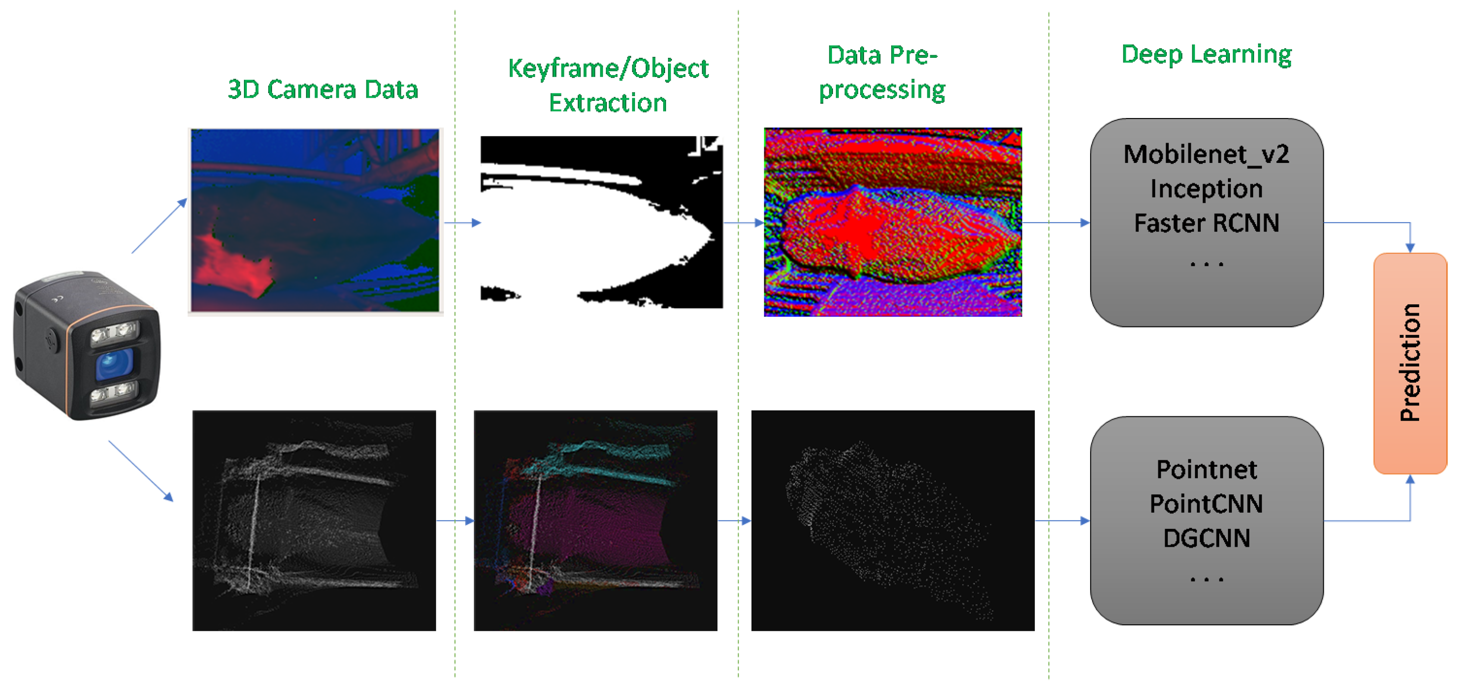
Figure 5.
Summary of the data and processes collected/implemented in this study.

Figure 6.
Depth-based foreground Segmentation: (a) depth image in greyscale, (b) result of applying amplitude OTSU thresholding a method widely used in classic image segmentation (c) extraction of contour with largest area (d) example of erroneous segmentation result where there is a separation of contours generated over the cow due to artefacts caused by cow coat patterns (visible in (b)) drawing a line across the cow.

Figure 7.
Colour Thresholding Process (a) depth image shown in blue channel where not much gradient is visible, (b) LAB image which makes gradients and edges more visible and (c) thresholding result where sometimes rails are erroneously included if too close to the cow.
Figure 7.
Colour Thresholding Process (a) depth image shown in blue channel where not much gradient is visible, (b) LAB image which makes gradients and edges more visible and (c) thresholding result where sometimes rails are erroneously included if too close to the cow.

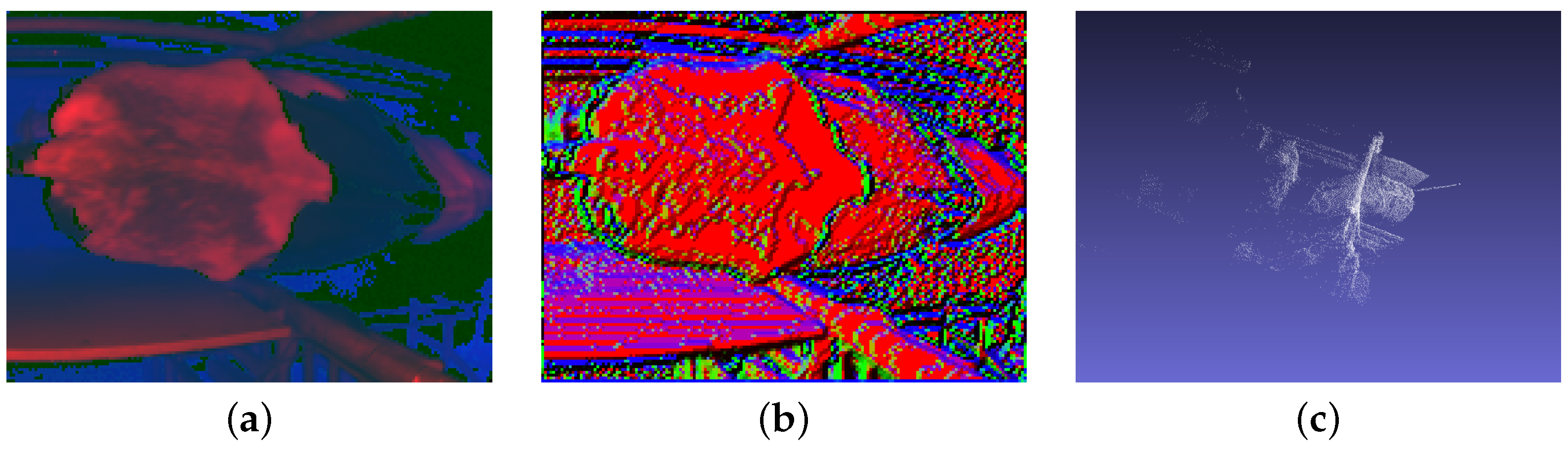
Figure 8.
Normal Map Calculation of cow’s back for (a) the entire depth image and (b) the segmented depth image.
Figure 8.
Normal Map Calculation of cow’s back for (a) the entire depth image and (b) the segmented depth image.

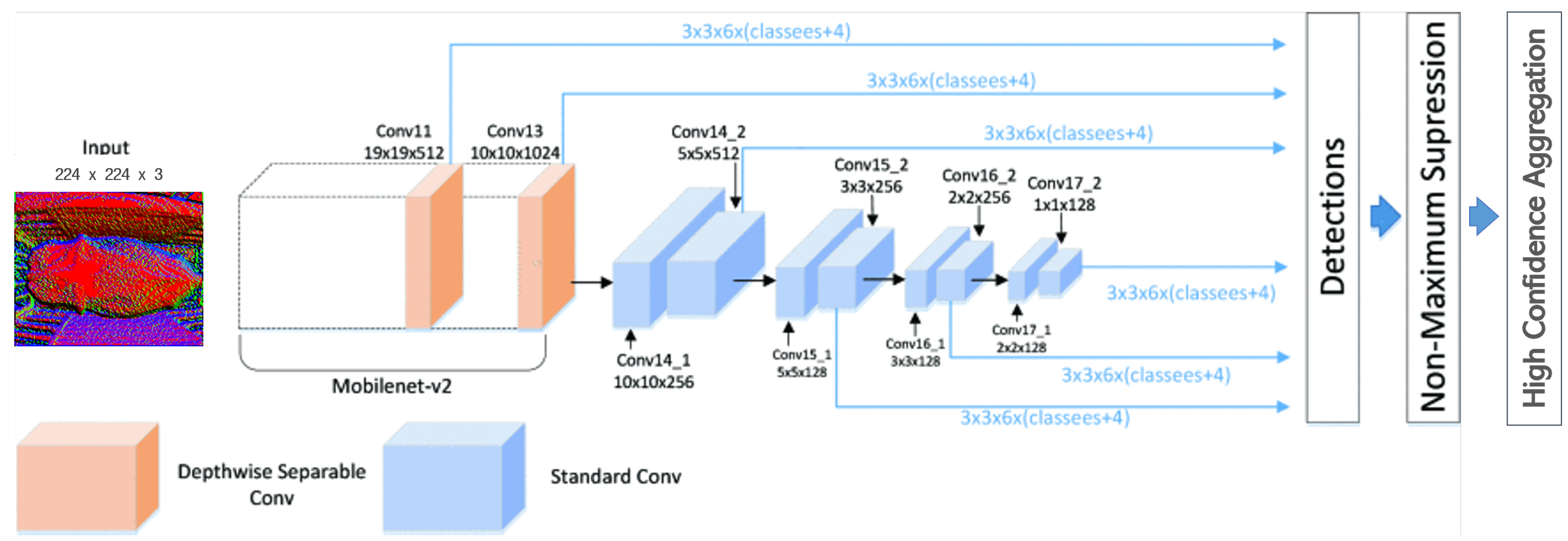
Figure 9.
The MobileNet-SSDv2 Network Architecture showed best results for the pre-processed normal map of the depth image. Image modified from [35].
Figure 9.
The MobileNet-SSDv2 Network Architecture showed best results for the pre-processed normal map of the depth image. Image modified from [35].

Figure 10.
The depth map from a different angle (a) produces a significantly different normal map (b) but the point cloud representation (c) remains the same as it would regardless of camera pose.
Figure 10.
The depth map from a different angle (a) produces a significantly different normal map (b) but the point cloud representation (c) remains the same as it would regardless of camera pose.

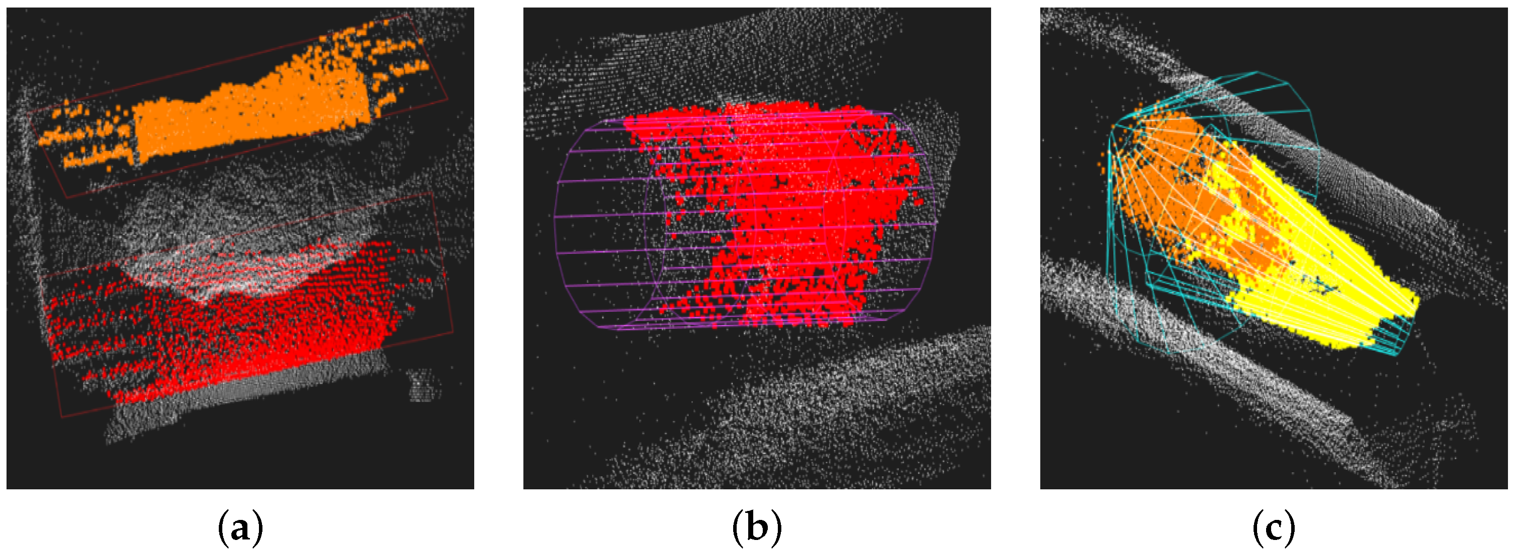
Figure 11.
Some successful instances of (a) plane, (b) cylinder and (c) cone segmentation required very tight constraints on shape dimensions which were not generalisable to all cows.
Figure 11.
Some successful instances of (a) plane, (b) cylinder and (c) cone segmentation required very tight constraints on shape dimensions which were not generalisable to all cows.

Figure 12.
Region-growing segmentation results.

Figure 13.
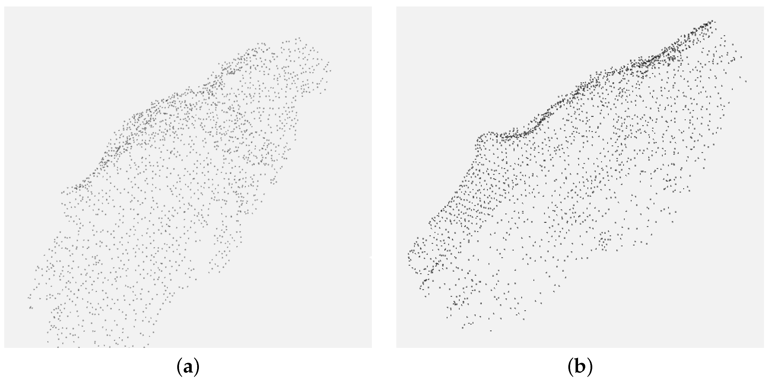
Subsampling results of (a) Random subsampling vs. (b) Normal-Space Subsampling.

Figure 14.
A visual representation of our comparison of 2D and 3D Deep Learning approaches to the BCS application.
Figure 14.
A visual representation of our comparison of 2D and 3D Deep Learning approaches to the BCS application.

Figure 15.
Confusion Matrix of BCS predictions.

Figure 16.
The 2D/3D DL Model Development Progress in BCS Classification.

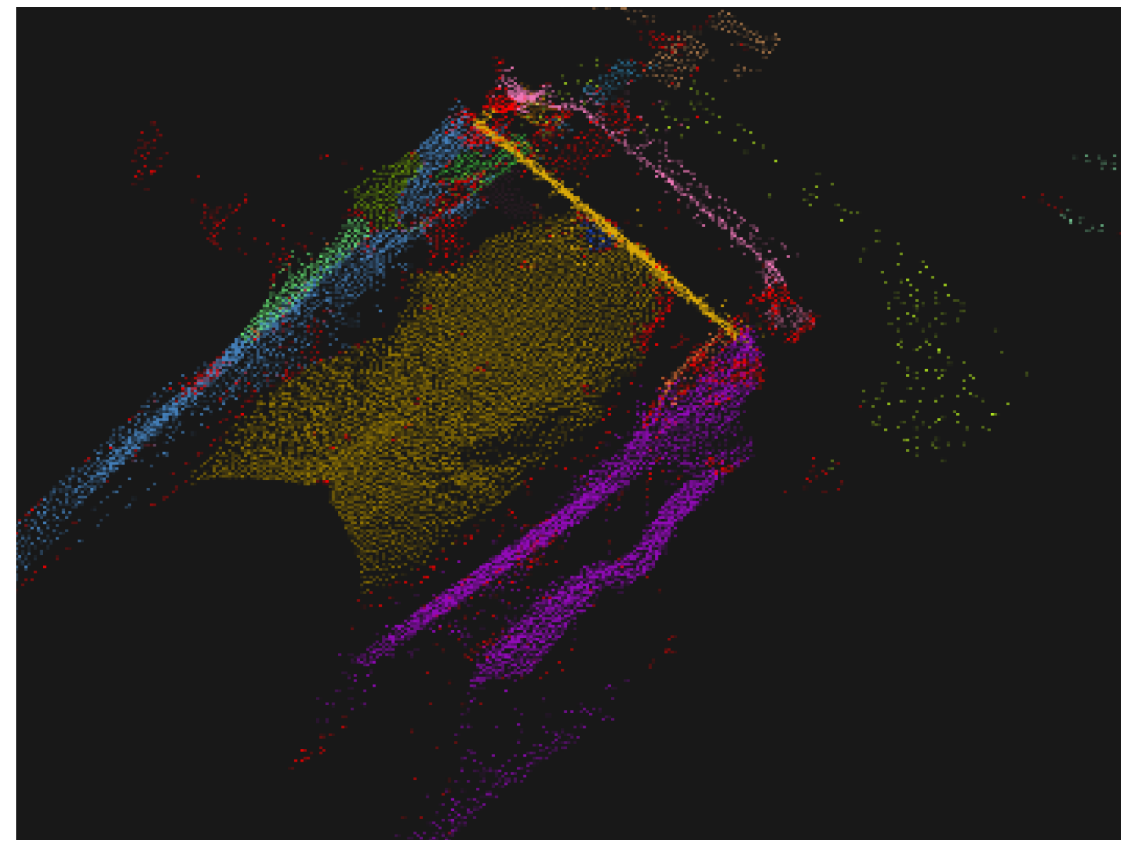
Figure 17.
PointNet Segmentation Results on patch at seed point and complete scene.

Figure 18.
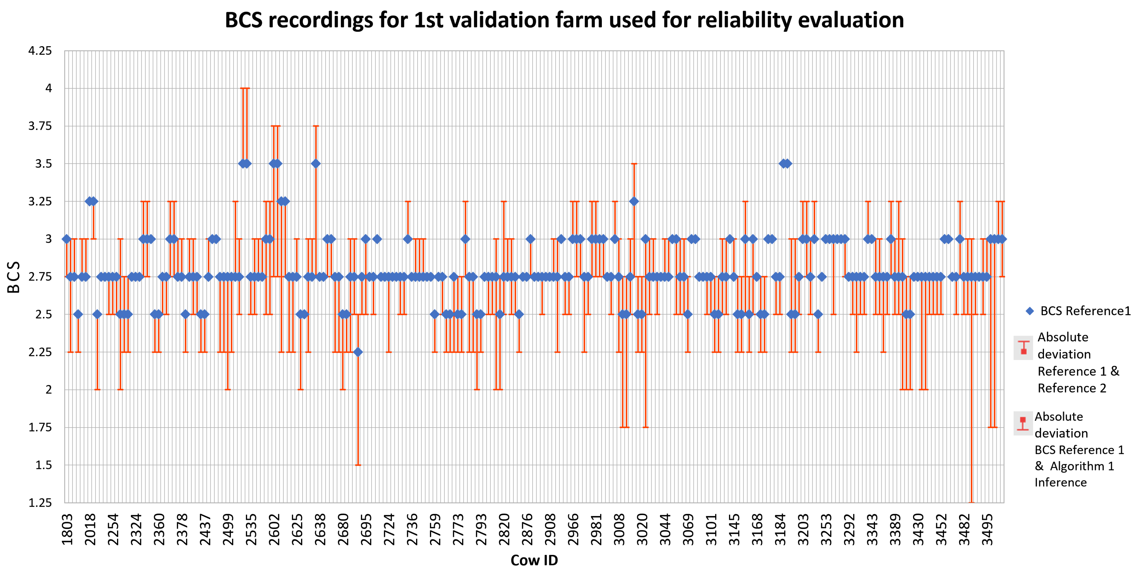
Plot of scores recorded vs. predictions for entire herd on validation farm using model trained with Algorithm 1 on research farm. Upper error bar values represent the deviation between the two vets (BCS Reference 1 vs. BCS Reference 2) and lower error bar values represent the deviation between one of the vets and Algorithm 1 (BCS Reference 1 vs. Algorithm 1).
Figure 18.
Plot of scores recorded vs. predictions for entire herd on validation farm using model trained with Algorithm 1 on research farm. Upper error bar values represent the deviation between the two vets (BCS Reference 1 vs. BCS Reference 2) and lower error bar values represent the deviation between one of the vets and Algorithm 1 (BCS Reference 1 vs. Algorithm 1).

Figure 19.
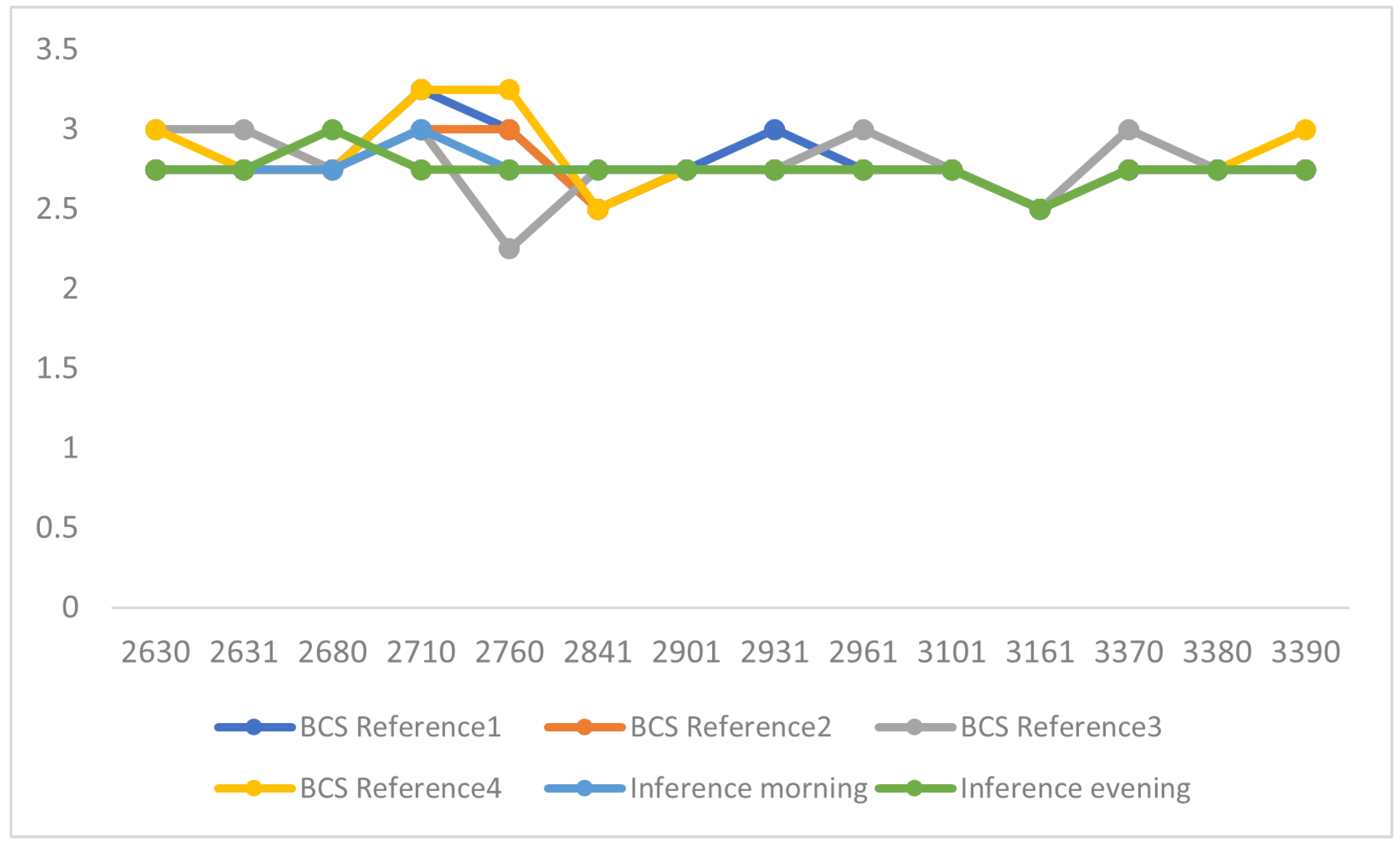
Morning/Evening Repeatability Analysis on 1st validation farm using model trained with Algorithm 1 on research farm and validation farm.
Figure 19.
Morning/Evening Repeatability Analysis on 1st validation farm using model trained with Algorithm 1 on research farm and validation farm.

Figure 20.
Radar chart of Intra/Inter Rater Agreement in BCS assessment of each of the validation farms.
Figure 20.
Radar chart of Intra/Inter Rater Agreement in BCS assessment of each of the validation farms.


Table 1.
Past Vision-based BCS Scoring Research.
| Features | Reference | Images in Dataset | Automated/ 3D/2D | Performance |
|---|---|---|---|---|
| Hook angle, posterior hook angle, depression | [6] | 834 | No/2D | 92.79 (note manual input is required) |
| Goodness of fit of a parabolic shape of the segmented image | [7] | 172 | Yes/2D | R = 0.94 |
| Measurement between specific points on a cows back | [8] | - | No/3D | Area estimate only |
| Principal Component Analysis | [9] | 25 | No/3D | R = 0.96 |
| 14 individual features per cow, derived from cows’ topography | [10] | 2650 | Yes/3D | 74% accurate within 0.25 |
| Area around the tailhead and left and right hooks | [11] | 130 | Yes/2D | Area estimate only |
| Body mass, hip height and withers height | [12] | 107 | Yes/3D | R2 = 0.946 (body mass estimation) |
| 3D surface of cows back and fitted sphere | [13] | 95 | Yes/3D | Area estimate only |
| Features determined by CNN on pre-processed depth images | [14] | 503 | Yes/3D | 0.78 accurate within 0.25 |
| Proprietary BCS system | [15] | 344 | Yes | 0.76 correlation |
| Refinement of [15] with smoothing filter | [16] | 32 | Yes | 0.86 Pearson correlation |
| Manual body measurements | [17] | 55 | No | R2 of 0.63 and RMSE of 0.16 |
Table 2.
BCS Classification Results with Tensorflow Object Detection models.
| Input Data | Location | Model | Inference Time (ms) | Classification Accuracy |
|---|---|---|---|---|
| IP Camera RGB Image | Drafting crate | Mobilenet V2 | 62 | 0.25 |
| Depth Image | Drafting crate | Mobilenet V2 | 30 | 0.26 |
| Depth Image | Drafting crate | Inception | 50 | 0.24 |
| Composite Image | Drafting crate | Mobilenet V2 | 30 | 0.29 |
| Normal Map | Drafting crate | Mobilenet V2 | 30 | 0.39 |
| Normal Map | Drafting crate | Mobilenet V1 FPN | 30 | 0.38 |
1 when ran on an intel i7 CPU and NVidia GTX 1060 graphics card; 2 when tested on a test set of cows not seen during training but part of the same herd.
Table 3.
A quantitative comparison of 3D deep neural networks in BCS classification.
| Input Data | Location | Preprocessing | Model | Classification Accuracy |
|---|---|---|---|---|
| Convolution-based | Rotary | Region-growing segmentation + outlier removal + Normal-Space Subsampling | Relation-Shape CNN | 0.185 |
| Graph-based | Rotary | Region-growing segmentation + outlier removal + Normal-Space Subsampling | DGCNN | 0.205 |
| Convolution-based | Rotary | Region-growing segmentation + outlier removal + Normal-Space Subsampling | PointCNN | 0.394 |
| Point-based | Draft | Region-of-Interest segmentation + minor Normal-Space Subsampling + block merging | Pointnet++ | 0.53 |
Table 4.
Correlation Matrix between the two human observers on the day of scoring on the 2nd validation farm. The five values in each cell correspond to Krippendorff’s coefficient, accuracy, accuracy within 0.25, accuracy within 0.5, accuracy within 0.75 and accuracy within 1.0 BCS in that order.
Table 4.
Correlation Matrix between the two human observers on the day of scoring on the 2nd validation farm. The five values in each cell correspond to Krippendorff’s coefficient, accuracy, accuracy within 0.25, accuracy within 0.5, accuracy within 0.75 and accuracy within 1.0 BCS in that order.
| Rater 1a | Rater 1b | Rater 2a | Rater 2b | Algorithm 1a | Algorithm 1b | Algorithm 2a | Algorithm 2b | |
|---|---|---|---|---|---|---|---|---|
| Rater 1a | 1.0000 | |||||||
| Rater 1b | 0.4920 | 1.0000 | ||||||
| 0.6890 | ||||||||
| 1.0000 | ||||||||
| 1.0000 | ||||||||
| 1.0000 | ||||||||
| Rater 2a | 0.2270 | 0.2850 | 1.0000 | |||||
| 0.4750 | 0.5250 | |||||||
| 0.9340 | 0.9180 | |||||||
| 0.9840 | 1.0000 | |||||||
| 1.0000 | 1.0000 | |||||||
| Rater 2b | 0.1570 | 0.1900 | 0.3950 | 1.0000 | ||||
| 0.4750 | 0.5080 | 0.6070 | ||||||
| 0.9180 | 0.9180 | 0.9020 | ||||||
| 1.0000 | 0.9840 | 0.9670 | ||||||
| 1.0000 | 1.0000 | 1.0000 | ||||||
| Algorithm 1a | −0.1683 | −0.2307 | −0.2228 | −0.2228 | 1.0000 | |||
| 0.1633 | 0.1224 | 0.0612 | 0.0612 | |||||
| 0.6735 | 0.6531 | 0.4286 | 0.4286 | |||||
| 0.8776 | 0.8980 | 0.7959 | 0.7959 | |||||
| 0.9796 | 1.0000 | 0.9388 | 0.9388 | |||||
| Algorithm 1b | −0.1412 | −0.2074 | −0.1950 | −0.2076 | 0.1570 | 1.0000 | ||
| 0.1429 | 0.1020 | 0.0408 | 0.0612 | 0.4750 | ||||
| 0.4082 | 0.4490 | 0.2857 | 0.2653 | 0.9180 | ||||
| 0.8571 | 0.8776 | 0.6939 | 0.6531 | 1.0000 | ||||
| 1.0000 | 1.0000 | 0.8980 | 0.9184 | 1.0000 | ||||
| Algorithm 2a | −0.0530 | 0.0267 | −0.0339 | −0.0415 | −0.0003 | 0.0452 | 1.0000 | |
| 0.2857 | 0.3469 | 0.2245 | 0.2653 | 0.3265 | 0.3469 | |||
| 0.7551 | 0.7755 | 0.5510 | 0.5306 | 0.8571 | 0.7755 | |||
| 0.9796 | 1.0000 | 0.9184 | 0.8776 | 1.0000 | 0.9388 | |||
| 1.0000 | 1.0000 | 1.0000 | 1.0000 | 1.0000 | 1.0000 | |||
| Algorithm 2b | 0.0484 | 0.0118 | −0.0762 | 0.0290 | 0.3878 | 0.2245 | 0.3720 | 1.0000 |
| 0.3878 | 0.3673 | 0.2245 | 0.3878 | 0.8776 | 0.6939 | 0.5918 | ||
| 0.7551 | 0.8163 | 0.6327 | 0.8776 | 0.9592 | 0.9388 | 0.9592 | ||
| 1.0000 | 0.9796 | 0.8776 | 0.9592 | 1.0000 | 1.0000 | 1.0000 | ||
| 1.0000 | 1.0000 | 1.0000 | 1.0000 | 1.0000 | 1.0000 | 1.0000 |
Disclaimer/Publisher’s Note: The statements, opinions and data contained in all publications are solely those of the individual author(s) and contributor(s) and not of MDPI and/or the editor(s). MDPI and/or the editor(s) disclaim responsibility for any injury to people or property resulting from any ideas, methods, instructions or products referred to in the content. |
© 2022 by the authors. Licensee MDPI, Basel, Switzerland. This article is an open access article distributed under the terms and conditions of the Creative Commons Attribution (CC BY) license (https://creativecommons.org/licenses/by/4.0/).
Share and Cite
MDPI and ACS Style
O’Mahony, N.; Krpalkova, L.; Sayers, G.; Krump, L.; Walsh, J.; Riordan, D. Two- and Three-Dimensional Computer Vision Techniques for More Reliable Body Condition Scoring. Dairy 2023, 4, 1-25. https://doi.org/10.3390/dairy4010001
AMA Style
O’Mahony N, Krpalkova L, Sayers G, Krump L, Walsh J, Riordan D. Two- and Three-Dimensional Computer Vision Techniques for More Reliable Body Condition Scoring. Dairy. 2023; 4(1):1-25. https://doi.org/10.3390/dairy4010001
Chicago/Turabian StyleO’Mahony, Niall, Lenka Krpalkova, Gearoid Sayers, Lea Krump, Joseph Walsh, and Daniel Riordan. 2023. "Two- and Three-Dimensional Computer Vision Techniques for More Reliable Body Condition Scoring" Dairy 4, no. 1: 1-25. https://doi.org/10.3390/dairy4010001