SAS PROC IRT and the R mirt Package: A Comparison of Model Parameter Estimation for Multidimensional IRT Models

Abstract

This study investigates the performance of estimation methods for multidimensional IRT models with dichotomous and polytomous data in two well-known IRT programs: SAS PROC IRT and the mirt package in R. A simulation study was used to compare performance on a simple structure Rasch model, complex structure 2PL model, and bifactor graded response model. Under RMSE and bias criteria regarding item parameter recovery, PROC IRT and mirt showed nearly identical performance in the simple structure condition. When a complex structure was used, mirt performed better in terms of the recovery of intercept parameters, while the recovery of slope parameters depended on the program and the sample sizes: PROC IRT tended to be better with small samples ($N=500$) according to RMSE, and mirt was better for larger samples ($N=1000$ and $2500$) according to RMSE and bias for the slope parameter recovery. When a bifactor structure was used, mirt was preferred in all cases; differences lessened as sample size increased.

1. Introduction

Recently, SAS/STAT^® software introduced the IRT analysis module PROC IRT [1], which complements existing software that specializes in item response theory (IRT) analysis (e.g., IRTPRO [2], flexMIRT [3]). Additionally, IRT model estimation programs under the freely available statistical computing environment, R [4], became available and widely used in research. Both SAS/STAT software and R IRT programs offer multidimensional model estimation capacity. The popularity of and demand for multidimensional IRT modeling has increased because it is not uncommon to find a test which measures more than a single construct, and it provides an effective means to handle user-defined multidimensional structures (e.g., a simple structure with correlated subtests in a test battery).

In research and practice, one may consider either SAS/STAT PROC IRT or an IRT package in R for the estimation of a multidimensional model. Some information on the performance of the two IRT model programs are available in terms of unidimensional modeling (e.g., [5,6,7,8]), but comparisons of estimating multidimensional models by SAS/STAT PROC IRT and R package(s) are still scarce. The purpose of this study is to generate comparative information on the performance of SAS/STAT PROC IRT and R IRT programs in terms of multidimensional IRT model estimation. The package (or program) for the estimation of multidimensional IRT models in R used in this study is mirt [9]. SAS/STAT software is a licensed software, charging users a fee for use, and performs a comprehensive set of statistical procedures, including PROC IRT for uni- and multidimensional IRT analyses. The R software is a freely available, open-source software with the mirt package available for performing uni- and multidimensional IRT analyses.

The next section introduces comparisons of the overall features in SAS/STAT PROC IRT and the R mirt package, followed by a simulation study.

Features

Both PROC IRT in SAS/STAT and the mirt package in R can perform Rasch models, one-, two-, three-, and four-parameter models, and graded response and generalized partial credit models for unidimensional and multidimensional structures. The nominal response model can be used for unidimensional data with PROC IRT or for uni- and multidimensional data with mirt. Both assume person latent scores are from a normal distribution, utilizing the marginal maximum likelihood (MML) estimation with an expectation-maximization (EM) or Newton-type algorithms for parameter estimations as their default estimation approaches [1,10,11]. Mirt provides additional estimation options. Both provide maximum likelihood (ML), maximum a posteriori (MAP), and expected a posteriori (EAP) as person ability (or latent trait) score estimators.

SAS/STAT PROC IRT applies the logit link function when calibrating data, along with the quasi-newton maximization method and adaptive quadrature approximation method, by default. Mirt, by default, utilizes a standard expectation maximization with fixed quadrature.

Table 1. Table of features for PROC IRT in SAS/STAT and mirt in R.

	PROC IRT in SAS/STAT	mirt in R
Models supported
Polytomous extensions	Graded response, generalized partial credit	Graded response, generalized partial credit
Dimensionality	Unidimensional, multidimensional	Unidimensional, multidimensional
Calibration
Link function	Logit, Probit	Logit
Model identification	$\theta ~N\left(0,1\right)$ or $N\left(0,{\sigma }^2\right)$ for Rasch modeling	$\theta ~N\left(0,1\right)$ or $N\left(0,{\sigma }^2\right)$ for Rasch modeling
Item calibration	MML as default	MML as default
Person ability	ML, EAP, MAP	EAP, MAP, ML, Weighted Likelihood Estimate (WLE)
Output
Global/Model fit	Log likelihood, Akaike’s and Bayesian information criterion, the likelihood ratio Chi–Square $G^2$ statistic, and Pearson’s Chi–Square	Log likelihood, Akaike’s and Bayesian information criterion, the likelihood ratio Chi–Square $G^2$ statistic, root mean square error of approximation (RMSEA), and $M_2$ test
Item fit	Likelihood Ratio $G^2$, Pearson’s Chi–Square Statistics	$S-X^2$ as default. Infit and outfit item fit statistics possible for the Rasch model
Person fit	None	Infit and outfit measures, and $l_z$
Plots	Item Information Curve, Test Information Curve, Item Characteristic Curve	Item Information Curve, Test Information Curve, Item Characteristic Curve
Other
Mixed format data	Yes	Yes
Missing data code	Blank, user-specified	‘NA’ used
Item parameter priors	Yes for the slope, the guessing, and the ceiling parameters for the 3PL and 4PL models only	Yes for the slope, the intercept, the guessing, and the ceiling parameters
Multiple-group IRT	Yes	Yes
Mixture models	No capability	Yes

Note. Missing data in R are specified with ‘NA’ (not available).

and

Table 2. Table of estimation features for PROC IRT in SAS/STAT and mirt in R.

	PROC IRT in SAS/STAT	mirt in R
Estimation Method	Conjugate-gradient	Block & Lieberman approach
	Expectation-Maximization (EM)	Expectation-Maximization (EM) *
	Newton-Rhaphson with ridging	Metropolis-Hastings Robbins-Monro (MHRM)
	Quasi-Newton *	Monte Carlo EM
		Stochastic EM
		Quasi-Monte Carlo EM
Quadrature Approximation	Adaptive Gauss-Hermite (G-H) *	Fixed quadratures *
	Gauss-Hermite (G-H)	Custom quadratures (or user-specified quadratures)
	Nonadaptive Gaussian Quatrature

* denotes the default setting.

below provide summaries of the features of the two programs. Note that in Table 1 and Table 2, we listed what we considered essential for beginners; furthermore, the two programs have a much wider scope of options regarding the details of model estimation specification and the directions of details of those option specifications are not identical. Thus, we recommend that one should further study the currently available information in “help” in R and the SAS/STAT documentation if they are interested in knowing the details at a deeper level.

The PROC IRT software and R mirt package have various algorithms for maximizing the marginal likelihood to obtain the model parameter estimates.

2. Materials and Methods

This study utilized a simulation study of three different multidimensional data structures (simple, complex, and bifactor; see

Table 3. Simulated multidimensional structures and IRT models.

		Model
Number of Dimensions	Structure	Rasch	2PL	GR
3	Simple	X
	Complex		X
4	Bifactor			X

Note. 2PL = two parameter logistic; GR = graded response logistic.

) to compare the model parameter estimation procedures utilized by PROC IRT and mirt. The specifications of the estimation methods were the defaults, when applicable, provided by the two programs because they would be the most common types of choices when users in practice run a multidimensional model estimation. The use of the default means for the person ability parameters, $\theta$, is assumed to follow a multivariate normal distribution and no distributional assumptions are made for the item parameters, i.e., there is no prior for item parameters in either program. PROC IRT does provide priors on the slope, guessing, and ceiling parameters when the 3PL and 4PL models are used.

The three structures have 30 items each. The multidimensional 2PL (M2PL) model used for data generation has the form $a^{\prime }\theta +d$, i.e., a compensatory MIRT model form, where the slope and person ability parameters across dimensions are $a^{\prime }$ and $\theta$, respectively, and the item intercept parameter is $d$. For the data simulation, the slope parameters were from a log-normal distribution with the mean equal to zero and a standard deviation ($SD$) of 0.2; this results in slope parameters which are always positive (common in IRT) and lie approximately between 0.5 and 2.0. The intercept parameter was from the standard normal distribution. Item specifications were taken from Cole and Paek [7]. For all conditions, sample sizes of $N=500, 1000$, and $2500$ were used. The number of replications was 100.

In R, mirt uses the slope-plus-intercept form, $a^{\prime }\theta +d$. SAS/STAT PROC IRT for the 2PL model and the GR model follow the slope-minus-intercept form, $a^{\prime }\theta -d$.

2.1. Simulation 1: Simple Structure with Rasch Model

The first simulation utilized a simple structure dataset of 30 items with dichotomous data, following a Rasch model. Three-dimensional data were composed of three 10-item subsets as follows: items 1–10 loaded only on the first dimension, items 11–20 loaded only on the second dimension, and items 21–30 loaded only on the third dimension. Correlation of dimensions were in the moderate range ($r_{12}=0.5, r_{13}=0.7, r_{23}=0.6$). For the model identification, the mean for each dimension was fixed to zero while the variances and the covariances of dimensions were estimated freely.

The person ability parameters ($\theta$s) of the simulated data were drawn from the tri-variate normal distributions with the mean equal to zero on all dimensions. The covariance matrix fixed the diagonals to ones and the off-diagonals to the correlation values addressed above. The intercept parameters were drawn from the standard normal distribution; these are the difficulty parameters in the simple structure Rasch model.

2.2. Simulation 2: Complex Structure with 2PL Model

The second simulation utilized a structure dataset of 30 items with dichotomous data following the 2PL model. Three-dimensional data were composed of three 10-item subsets as follows: items 1–10 loaded only on the first dimension, items 11–20 loaded only on the second dimension, and items 21–30 loaded on all three dimensions. Correlation of dimensions were in the moderate range ($r_{12}=0.5, r_{13}=0.7, r_{23}=0.6$). Model identification specifications were similar to the first simulation.

The person ability parameters and intercept parameters of the simulated data were drawn from the same tri-variate normal distribution used in the above Rasch model condition. A log-normal distribution was utilized for the slope parameters, with its mean equal to 0.25 and its standard deviation equal to 0.25.

2.3. Simulation 3: Bifactor Structure with Graded Response Model

The third and final simulation utilized a bifactor structure dataset of 30 items with polytomous data with 3 categories, following the GR model. Four-dimensional data were composed such that all 30 items loaded on a common general factor along with three 10-item subsets as follows: items 1–10 loaded only on the first specific dimension, items 11–20 loaded only on the second specific dimension, and items 21–30 loaded only on the third specific dimension. Across factors, the mean and the variance were fixed to zero and one, respectively. The dimensions were uncorrelated.

Person ability parameters were drawn from a multivariate normal distribution with zero means across dimensions, and the covariance matrix corresponded to the identity matrix with n = 4. Similar to the second simulation, the slope parameters were drawn from the same lognormal distribution. The item intercept parameters for the three categories, $d_1$ and $d_2$, were drawn from two uniform distributions ranging from (−2, 0) and (0, 2), respectively.

2.4. Computer Specifications

The computer specifications were an Intel^® Core^TM i5-6500 CPU at 3.20 GHz with 8 GB of physical RAM. The operating system was Microsoft Windows 10 Enterprise. For IRT calibrations in SAS, 9.4 with the SAS/STAT^® 14.1 component was used. In this study the R version was 4.2.2. and the mirt version was 1.38.1.

2.5. Evaluation

Evaluation was conducted in terms of run time, bias and RMSE of item parameter estimates, and the population parameter estimates (e.g., variances in the case of simple Rasch models and covariances among dimensions in the case of the simple Rasch and complex 2PL models). Regarding the item parameter recovery, the averages of bias and RMSE across items for the slope and the intercept parameters, respectively, are reported as summative evaluation measures for each data-simulation condition. In addition, we report the convergence (or non-convergence) rates as a side for practical information. The convergence criterion used in this study were the program defaults (when applicable), while the default model parameter estimation methods were chosen as mentioned before. When calibrating the complex and bifactor models, the calibrations converged with extremely incorrect parameter estimates in the SAS/STAT PROC IRT runs. The authors communicated with SAS/STAT technical specialists, and it was recommended to loosen the convergence criterion, which yielded more practical estimates. (See note a under

Table 4. Average run time (in seconds) and convergence rates.

		$\mathbf{Run} \mathbf{Time}: \mathit{M}\left(\mathit{S}\mathit{D}\right)$				Convergence (%)
Data Format	Sample Size	PROC IRT		mirt		PROC IRT a	mirt
Simple	500	25.75	(1.55)	70.11	(14.69)	100	100
	1000	39.25	(14.67)	95.39	(7.49)	100	100
	2500	69.19	(44.43)	176.55	(6.41)	100	100
Complex	500	45.45	(20.97)	66.46	(32.88)	100 a	97
	1000	103.36	(64.94)	67.61	(12.42)	100 a	99
	2500	112.90	(74.07)	115.89	(7.31)	100 a	100
Bifactor	500	2318.46	(1232.00)	26.24	(1.50)	100 a	100
	1000	1890.47	(1078.33)	39.74	(1.26)	100 a	100
	2500	3115.67	(372.19)	76.58	(1.80)	100 a	100

^a The PROC IRT convergence for the simple structure converged at the default 1 × 10⁻⁸. The complex and bifactor models did converge but with extreme errors in item parameter estimations. Communication with SAS/STAT technical specialists suggested loosening the convergence to 1 × 10⁻⁵. The complex and bifactor models converged with a converge criterion of 1 × 10⁻⁵.

for the convergence rules used in the study.) Within R, the default convergence was used.

Appendix A provides the SAS/STAT PROC IRT and R syntax used for calibrating datasets.

3. Results

3.1. Run Time and Convergence

Table 4 presents the mean and standard deviation of the run time for each simulation using SAS/STAT PROC IRT and R mirt and the percentage of convergence (out of 100 repetitions). PROC IRT performed quicker when a simple structure was used at all levels of sample size and when a complex structure was used with a sample size of $N=500$ and $N=2500$. R performed quicker when a complex structure was used with a sample size of $N=1000$, and R performed considerably faster for the bifactor structure at all levels of sample size. All simulations converged using R for the simple and bifactor structures; when a complex structure was used, convergence rates were 97%, 99%, and 100% for the sample sizes of $N=500, 1000,$ and $2500$, respectively. All simulations converged using PROC IRT at the default convergence criterion (1 × 10⁻⁸) for the simple structure, and at the loosened criterion (1 × 10⁻⁵) for the complex and bifactor structures.

The faster run time of mirt is most likely due to the employment of the dimension reduction technique for the bifactor model estimation using the mirt::bfactor() function, which is not available in PROC IRT for the bifactor model estimation.

3.2. Recovery of Item Parameters

3.2.1. Simple Structure with Rasch Model

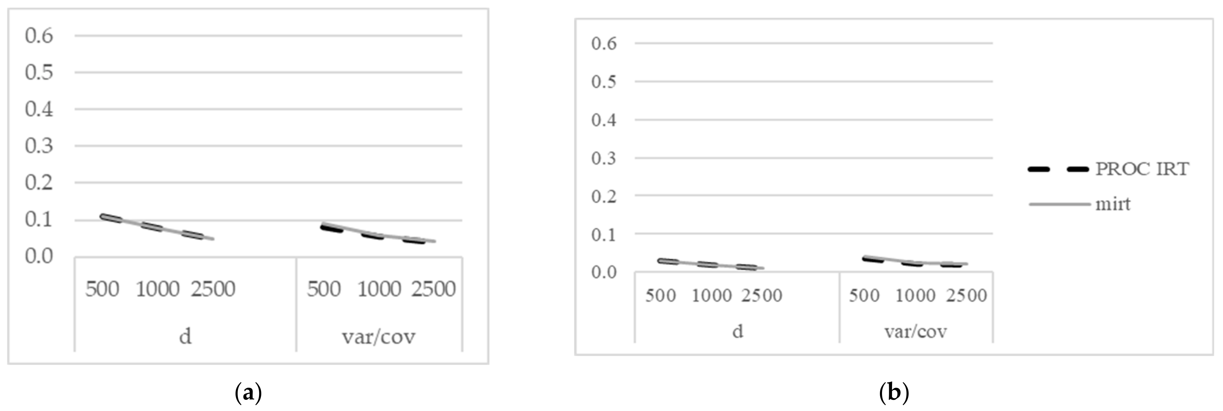
All cases met convergence in both mirt and PROC IRT.

Table 5. RMSE and bias of item parameters for the simple structure with Rasch model.

Data Format	Sample Size	Par	PROC IRT		mirt
			RMSE	Bias	RMSE	Bias
Simple	500	$d$	0.109	0.030	0.109	0.030
		var/cov	0.082	0.037	0.090	0.040
	1000	$d$	0.076	0.018	0.076	0.018
		var/cov	0.056	0.023	0.059	0.023
	2500	$d$	0.048	0.009	0.048	0.009
		var/cov	0.039	0.019	0.043	0.022

Note. var/cov refers to the estimated variance and covariance of the factors.

reports the RMSE and bias, and Figure 1a,b display the measures.

PROC IRT and mirt had nearly identical performance of RMSE and bias for the intercept ($d$) parameter (RMSE ranged from 0.109 when $N=500$ to 0.048 when $N=2500$, and bias ranged from 0.030 when $N=500$ to 0.009 when $N=2500$) and very similar performance of the variance and covariances of factors (RMSE ranged from 0.090 when $N=500$ to 0.043 when $N=2500$, and bias ranged from 0.040 when $N=500$ to 0.019 when $N=2500$). The RMSE and bias of the variance and covariances of the factors were slightly higher in mirt as compared to PROC IRT. As sample size increased, measures of error decreased.

3.2.2. Complex Structure with 2PL Model

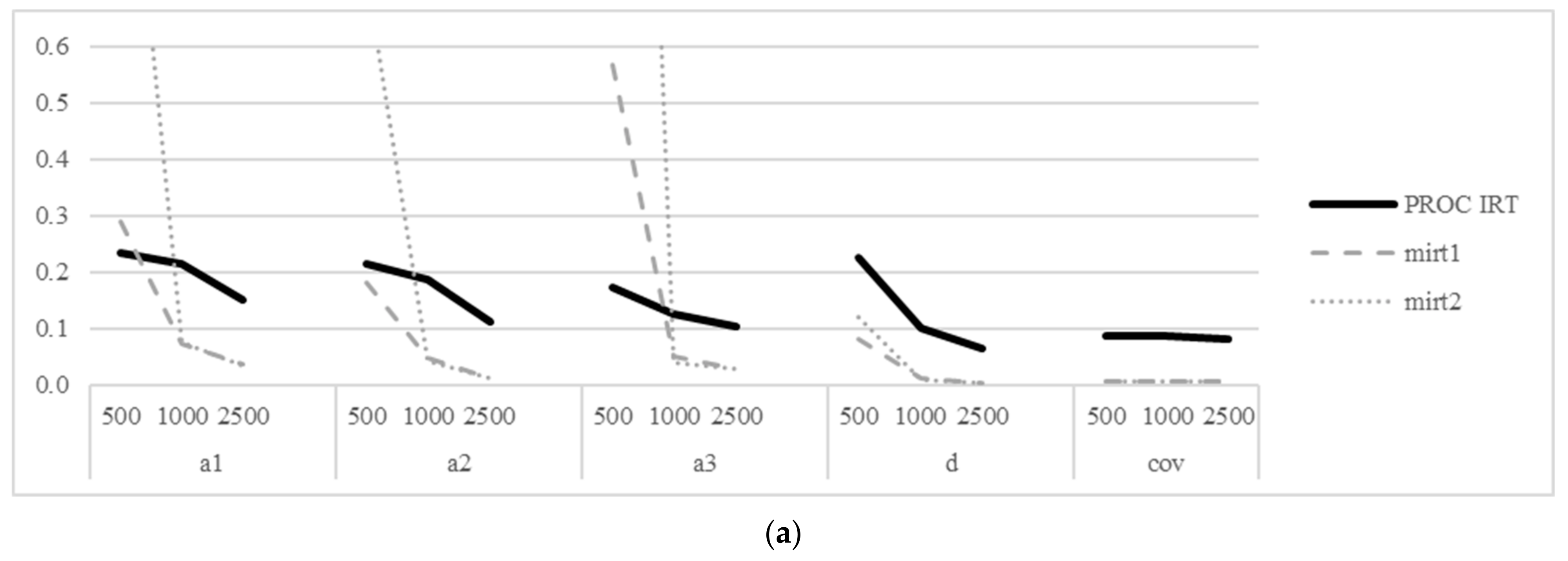
In mirt, nearly all replications reached the default convergence check (97%, 99%, and 100% for the sample sizes of 500, 1000, and 2500, respectively).

Table 6. RMSE and bias of item parameters for the complex structure with 2PL model.

Data Format	Sample Size	Par	PROC IRT		mirt
			RMSE	Bias	RMSE	Bias
Complex	500	$a_1$	0.234	0.138	0.292	0.069
		$a_2$	0.214	0.125	0.181	0.031
		$a_3$	0.173	0.065	0.569	0.017
		$d$	0.227	0.170	0.082	0.049
		cov	0.087	0.078	0.007	0.007
	1000	$a_1$	0.214	0.165	0.075	0.050
		$a_2$	0.187	0.134	0.050	0.029
		$a_3$	0.127	0.052	0.050	0.011
		$d$	0.103	0.015	0.013	0.001
		cov	0.087	0.080	0.007	0.007
	2500	$a_1$	0.153	0.126	0.038	0.031
		$a_2$	0.113	0.074	0.014	0.008
		$a_3$	0.105	0.081	0.030	0.018
		$d$	0.066	0.021	0.005	0.001
		cov	0.083	0.075	0.007	0.007

Note. cov refers to the estimated covariance among factors. All PROC IRT replications reached convergence at a loosened 1 × 10⁻⁵ convergence criterion.

reports the RMSE and bias for PROC IRT and mirt for replications reaching convergence; these are displayed in Figure 2a,b. In PROC IRT, replications reached convergence at the default 1 × 10⁻⁸ convergence criterion; however, parameters were estimated with extreme errors (i.e., values greater than 10.0). SAS/STAT technical specialists recommended a loosened convergence criterion of 1 × 10⁻⁵, in which all cases reached convergence with reasonable estimates.

For mirt, the RMSE of the slope parameters, $a_1$ and $a_2$, were less than 0.30, but the RMSE of $a_3$ was higher (0.569). PROC IRT estimated all slope parameters less than 0.240 when a small sample size ($N=500$) was used. At larger sample sizes ($N=1000$ and $2500$), the RMSE of mirt tended to be low (less than 0.08) and less than that of PROC IRT (which ranged from 0.214 for $a_1$ and $N=1000$ to 0.105 for $a_3$ and $N=2500$).

At all levels of sample size, mirt had smaller RMSEs (less than 0.02) than PROC IRT (ranged from 0.103 to 0.083) when estimating the intercept and factor covariances.

Lastly, for all parameters and at all sample sizes, mirt estimated with low (less than 0.5) and smaller bias than PROC IRT (ranging from 0.165 to 0.015).

For all item parameters, when the complex structure using the 2PL model was applied, measures of error decreased as sample size increased (except for the case of estimating the bias of $a_3$ when $N=2500$, which increased slightly as sample size increased). Measures of error for the covariances were not affected by sample size.

3.2.3. Bifactor Structure with Graded Response Model

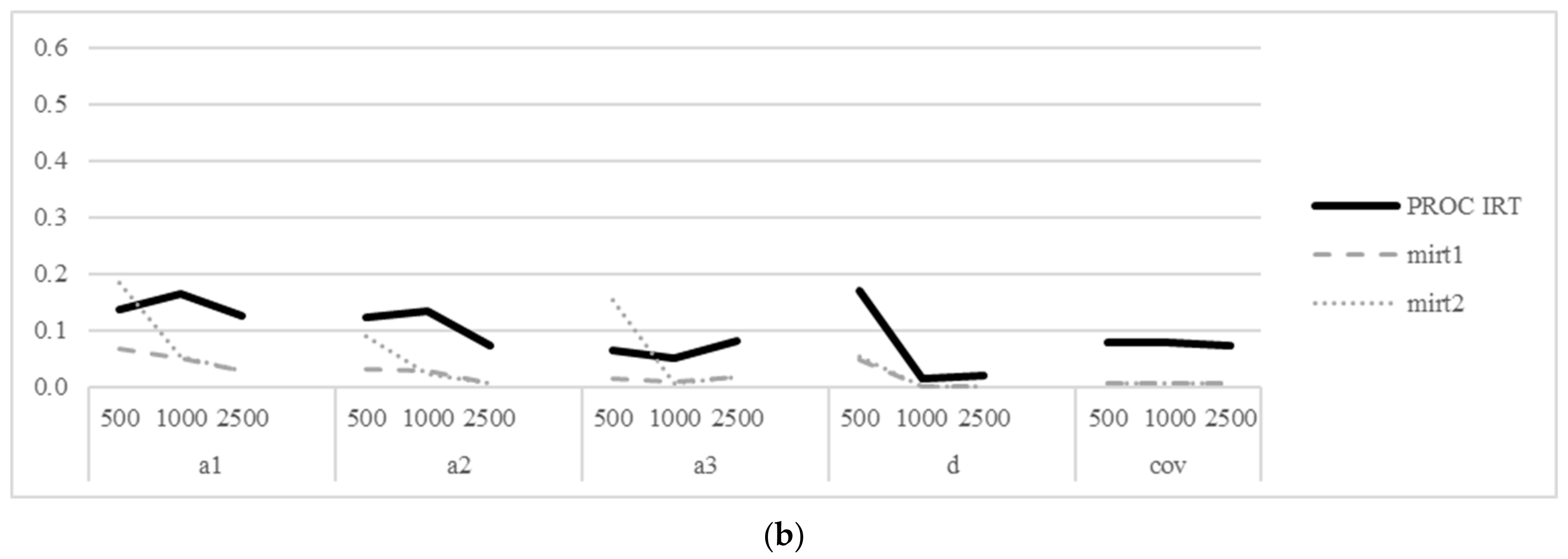
In mirt, all replications reached the default convergence check. In PROC IRT, replications reached convergence at the default 1 × 10⁻⁸ convergence criterion; however, parameters were estimated with extreme errors. As with the complex structure cases, SAS/STAT technical specialists recommended a loosened convergence criterion of 1 × 10⁻⁵, in which all cases reached convergence.

Table 7. RMSE and bias of item parameters for the bifactor structure with GRM model.

Data Format	Sample Size	Par	PROC IRT		mirt
			RMSE	Bias	RMSE	Bias
Complex	500	$a_1$	0.224	0.145	0.032	0.006
		$a_2$	0.130	0.100	0.014	0.000
		$a_3$	0.111	0.083	0.012	0.002
		$a_4$	0.120	0.096	0.017	0.006
		$d_1$	0.155	0.057	0.022	0.004
		$d_2$	0.135	0.036	0.018	0.003
	1000	$a_1$	0.124	0.052	0.016	0.005
		$a_2$	0.045	0.003	0.006	0.000
		$a_3$	0.046	0.017	0.005	0.000
		$a_4$	0.045	0.007	0.007	0.001
		$d_1$	0.099	0.037	0.010	0.002
		$d_2$	0.101	0.045	0.010	0.002
	2500	$a_1$	0.091	0.048	0.008	0.003
		$a_2$	0.042	0.031	0.003	0.001
		$a_3$	0.032	0.018	0.002	0.000
		$a_4$	0.031	0.014	0.002	0.000
		$d_1$	0.075	0.044	0.006	0.002
		$d_2$	0.072	0.041	0.005	0.002

Note. All mirt replications met the default convergence check. All PROC IRT replications reached convergence at a loosened 1 × 10⁻⁵ convergence criterion.

reports the RMSE and bias, and these are displayed in Figure 3a,b, respectively.

For all cases at all levels of sample size, mirt performed better in terms of RMSE and bias than PROC IRT. RMSE of mirt ranged from 0.032 (for $a_1$ when $N=500$) to 0.002 (for $a_3$ when $N=2500$). Bias of mirt ranged from 0.006 (for $a_1$ when $N=500$) to less than 0.001 for many cases. For all parameters in mirt, RMSE and bias were only slightly affected by sample size, decreasing as sample sizes increased.

PROC IRT had higher effects of sample size. When sample sizes were small ($N=500$), RMSE was very high (maximum of 0.224 for $a_1$), as was bias (maximum of 0.145 for $a_1$). At $N=2500$, RMSE decreased as low as 0.032 (for $a_3$ when $N=2500$) and bias decreased as low as 0.017 ($a_3,N=1000$).

4. Discussion and Conclusions

This study investigated performance of two IRT programs using their default estimation methods, given that practitioners or end-users are highly likely to employ the default setting. Although both programs use the MML estimation by default, some aspects of the estimation details are not the same. For example, stopping rules for the iterative process in the model estimation are different and SAS/STAT PROC IRT uses an adaptive quadrature (by default), while mirt does not. The adaptive quadrature approach attempts to optimally choose the number of quadratures and their locations, while mirt uses a fixed set of quadratures (e.g., 61 quadratures at [–6, 6] on theta). Thus, our comparison here necessarily involves these differences across the two programs.

The comparisons of both programs were made for multidimensional dichotomous and polytomous response data. Below are major observations from the simulations.

When dichotomous data followed the three-dimensional Rasch model with a simple structure, both PROC IRT and mirt produced virtually the same performance in terms of recovering model parameters (specifically, bias and RMSE) with the sample size greater than or equal to 500. In large scale assessment programs, the Rasch model is a popular choice and typically a sample size of a few thousand or greater is used for model calibration. Research-wise, smaller sample sizes (a few hundred) are sometimes used. Though the results should be cautiously interpreted, our current findings are encouraging in that when the sample size is at least 500 or greater, the preferences of PROC IRT and mirt are equal.

When dichotomous data followed a three-dimensional complex structure with the 2PL model, where some items were cross-loaded, PROC IRT and mirt showed some differences. When the results from the mirt’s default convergence rule were examined, except for the recovery of one of the slope parameters with N = 500, mirt performed better than PROC IRT regarding RMSE and bias. Overall, when sample sizes are large (i.e., greater than or equal to 1000), mirt (using the first default convergence) performs better than PROC IRT.

When polytomous data followed a four-dimensional bifactor GR model, mirt recovered model parameters better than PROC IRT across all sample size conditions, though the difference of performance decreased as sample size increased and the difference between both programs was small, in particular when sample sizes were 500 or higher.

The use of an adaptive quadrature is an approach that can boost the estimation speed in multidimensional model estimation. However, as the number of dimensions increases (say, four or greater), the adaptive quadrature approach should compromise between the model parameter estimation speed and the accuracy of model parameter estimation when reducing the number of quadratures for the multidimensional run. We conjecture that, in the cases of the complex and bifactor model estimation, this compromise is a part of the reason why PROC IRT tended to underperform for these conditions. In addition, the lack of the dimensional reduction technique [12,13,14] in PROC IRT seems to be another contributing factor in the lesser performance of PROC IRT compared to mirt for the bifactor structure condition. (Note again, mirt::bfactor() uses the dimension reduction technique.) Based on the orthogonal structure of a bifactor model, the dimension reduction technique essentially reduces the number of dimensions to two, regardless of the total number of dimensions in a bifactor model, so that it lessens the workload of the multidimensional model estimation. The use of the dimension reduction technique made dramatic differences in the run time as well (see Table 4).

We chose popular multidimensional structures such as a simple structure, a cross-loading (i.e., complex) structure, and a bifactor structure. In reality, data could be even more complex than what is covered in this study for their dimensional structures. Therefore, the exploratory multidimensional model estimation approach may be of interest and could be investigated further. Exploratory multidimensional modeling could entail a very high dimensional modeling for which the current default MML estimation in mirt and PROC IRT becomes less attractive due to the increasing workload for the model estimation as the number of dimension increases. Thus, a different model estimation approach such as the Metropolis–Hastings Robbins–Monro (MHRM) method [9,12,15] may be considered for more complex, high-dimensional modeling.

In addition to the coverage of the types of multidimensional structures and estimation approaches used in this study, more limitations exist in this study, and they could be addressed in future research. For example, the Rasch model is a popular choice, especially for its applications with small sample sizes. In a research setting, it may not be uncommon to observe a sample size of 500 or less. Therefore, a study that investigates performance of these IRT programs under smaller sample sizes (e.g., 150, 200, or 300) would be a worthwhile endeavor as well.

References

- SAS Institute Inc. SAS/STAT® 14.3 User’s Guide; SAS Institute Inc.: Cary, NC, USA, 2017. [Google Scholar]
- Vector Psychometric Group. IRTPRO for Windows V6 Computer Software; Vector Psychometric Group, LLC.: Chapel Hill, NC, USA, 2023. [Google Scholar]
- Houts, C.R.; Cai, L. flexMIRT User’s Manual Version 3.52: Flexible Multilevel Multidimensional Item Analysis and Test Scoring; Vector Psychometric Group: Chapel Hill, NC, USA, 2020. [Google Scholar]
- R Core Team. R: A Language and Environment for Statistical Computing; R Foundation for Statistical Computing: Vienna, Austria, 2023; Available online: https://www.R-project.org (accessed on 1 January 2023).
- Choi, J. A review of PROC IRT in SAS. J. Educ. Behav. Stat. 2017, 42, 195–205. [Google Scholar] [CrossRef]
- Cole, K.; Paek, I. PROC IRT: A SAS procedure for item response theory. Appl. Psychol. Meas. 2017, 41, 311–320. [Google Scholar] [CrossRef]
- Cole, K.; Paek, I. Using SAS PROC IRT for multidimensional item response theory analysis. Meas. Interdiscip. Res. Perspect. 2022, 20, 49–55. [Google Scholar] [CrossRef]
- Han, K.; Paek, I. A review of commercial software packages for multidimensional IRT modeling. Appl. Psychol. Meas. 2014, 38, 486–498. [Google Scholar] [CrossRef]
- Cai, L.S. Metropolis-Hastings Robbins-Monro algorithm for high-dimensional item response theory modeling. Psychol. Methods 2013, 18, 556–573. [Google Scholar]
- Bock, R.D.; Aitkin, M. Marginal maximum likelihood estimation of item parameters: Application of an EM algorithm. Psychometrika 1981, 46, 443–459. [Google Scholar] [CrossRef]
- Chalmers, R.P. mirt: A multidimensional item response theory package for the R environment. J. Stat. Softw. 2012, 48, 1–29. [Google Scholar] [CrossRef] [Green Version]
- Cai, L.S. Full-information item bifactor analysis using the EM algorithm. Psychol. Methods 2010, 15, 242–257. [Google Scholar]
- Gibbons, R.D.; Hedeker, D. A dimension reduction technique for bifactor analysis. Psychol. Methods 1992, 7, 192–204. [Google Scholar]
- Gibbons, R.D.; Hedeker, D. Generalized full-information item bifactor analysis. Psychometrika 2007, 72, 217–236. [Google Scholar]
- Cai, L.S. High-dimensional item response theory modeling. Psychometrika 2012, 77, 1–20. [Google Scholar]
Figure 1.
RMSE (a) and bias (b) of item parameter estimates for the simple structure with Rasch modeling.
Figure 2.
RMSE (a) and (b) bias of item parameters for the complex model.
Figure 3.
RMSE (a) and bias (b) of item parameters for the bifactor model.