Bayesian Estimation of Latent Space Item Response Models with JAGS, Stan, and NIMBLE in R

Abstract

The latent space item response model (LSIRM) is a newly-developed approach to analyzing and visualizing conditional dependencies in item response data, manifested as the interactions between respondents and items, between respondents, and between items. This paper provides a practical guide to the Bayesian estimation of LSIRM using three open-source software options, JAGS, Stan, and NIMBLE in R. By means of an empirical example, we illustrate LSIRM estimation, providing details on the model specification and implementation, convergence diagnostics, model fit evaluations and interaction map visualizations.

1. Introduction

Item Response Theory (IRT) is widely used for item response analysis in various fields, including education, psychology, medicine, and other social sciences, where assessments measure unobserved constructs, such as cognitive ability, personality, and mental well being. IRT provides a way to model the relationship between individuals’ responses to test items and the underlying construct being measured by the test. Conventional IRT models are based on a set of strong assumptions, such as conditional independence (i.e., responses are independent of one another, given the latent trait). However, conditional independence may not hold in real-life data analysis when unobserved interactions between respondents and items exist and are conditional on the latent trait.

Recently, Jeon et al. [1] introduced a novel latent space item response modeling (LSIRM) framework that relaxes the conditional independence assumption. LSIRM captures conditional dependencies unaccounted for by conventional IRT models [2] in terms of respondent-by-item interactions, where the interactions are modeled in the form of distances between respondents and items in a low-dimensional geometric space, called an interaction map. An estimated interaction shows conditional dependencies, or deviations from the Rasch model, for items and respondents, helping in the identification of intended or unintended response behaviors or in the evaluation of item grouping structures in comparison to the intended test design. In summary, the LSIRM approach has substantial technical advantages, due to its relaxing of the conditional independence assumption, and, by producing a geometrical representation of unobserved item–respondent interactions, it may supply important insights into the respondents and test items under investigation.

Jeon et al. [1] described a fully Bayesian approach with Markov chain Monte Carlo (MCMC) for estimating the original LSIRM. To facilitate the wider adoption and application of LSIRM in research and practice, we aim to provide a practical guide to LSIRM estimation using commonly used, free of charge, Bayesian software, such as JAGS [3,4,5], Stan [6,7], and NIMBLE [8,9] in R.

This paper begins with a brief description of LSIRM for binary response data and LSIRM parameter estimation with MCMC. We provide detailed R syntax for model specification and implementation in JAGS, Stan, and NIMBLE with a real-life data example. We also provide convergence and model fit diagnosis, run-time/sampling efficiency, and interaction map visualization comparison across the three packages. We conclude the paper with a summary and brief discussion.

2. Background

2.1. Latent Space Item Response Model

The original latent space item response model (LSIRM) [1] extended the Rasch model by introducing a respondent-by-item distance term from a p-dimensional space ${\mathcal{R}}^p$. LSIRM assumes that respondents and items have positions in the shared latent space ${\mathcal{R}}^p$. The distance between the respondent and item positions in the space indicates the interaction between the respondent and the item unexplained by the person and item parameters of the Rasch model. Specifically, LSIRM specifies the probability of giving a correct response by respondent j to item i as

$$\mathrm{logit}\left(\mathcal{P}(Y_{ji}=1|{\theta }_j,{\beta }_i,\gamma ,{\mathbf{z}}_j,{\mathbf{w}}_i)\right)={\theta }_j+{\beta }_i-\gamma d({\mathbf{z}}_j,{\mathbf{w}}_i),$$

(1)

where $\mathbf{Y}=\left\{y_{ji}\right\}$ is a N by I item response matrix, and $y_{ji}$ is the response of respondent j to item i ($j=1,2,\cdots ,N$ and $i=1,2,\cdots ,I$). When $\mathbf{Y}$ are all binary responses, we use $y_{ji}=1$ to denote an affirmative endorsement (e.g., correct, true, or yes) to the item, while $y_{ji}=0$ denotes no endorsement (e.g., incorrect, false, or no). ${\theta }_j\sim N(0,{\sigma }^2)$ is the person intercept or the main effect of respondent j that can be interpreted as respondent j’s latent trait being measured by the test. The value ${\beta }_i$ is the item intercept or the main effect of item i that can be interpreted as the item i’s easiness. The value $\gamma >0$ is the weight of the distance term that captures the overall degree of conditional dependencies in the item response data; a larger $\gamma$ indicates stronger evidence of conditional dependencies (i.e., violation of the conditional independence assumption) in the item response data under investigation, When $\gamma =0$, the model reduces to the Rasch model. $d({\mathbf{z}}_j,{\mathbf{w}}_i)$ is the distance function that measures pairwise distances between a respondent’s latent position ${\mathbf{z}}_j$ and an item’s latent position ${\mathbf{w}}_i$ in the p-dimensional Euclidean space ${\mathcal{R}}^p$ with known dimension p.

To facilitate visualization and interpretation, in this paper we use a two-dimensional Euclidean space ($p=2$) and Euclidean distance $d({\mathbf{z}}_j,{\mathbf{w}}_i)=\Vert d({\mathbf{z}}_j,{\mathbf{w}}_i)=\parallel {\mathbf{z}}_j-{\mathbf{w}}_i\parallel$, where a larger distance between ${\mathbf{z}}_j$ and ${\mathbf{w}}_i$ contributes to a lower probability of person j giving a correct response to item i, given the person’s overall trait level and the item’s overall easiness. As such, a distance between the respondent and item positions indicates a respondent-by-item interaction. When there is little interaction between respondents and items, all distances are near zero (i.e., all person and item positions are close to $(0,0)$ in a ${\mathcal{R}}^2$ space), as shown in [1]. In the sense that the latent space represents unobserved interactions, it is referred to as an interaction map [1]. Note that the interaction map is not an ability space; i.e., the coordinates of the space do not represent ability dimensions. Instead, the latent space is a tool to represent respondent-by-item interactions unexplainable by the parameters of the Rasch model. Other additional details of the model specifications, assumptions, and interpretations can be found in the original paper [1].

The likelihood function of the observed item response data $\mathbf{y}$ can be written as

$$\mathcal{L}(\mathbf{Y}=\mathbf{y}|\mathsf{\theta },\mathsf{\beta },\mathsf{\gamma },\mathbf{Z},\mathbf{W})=\prod _{j=1}^N\prod _{i=1}^I\mathcal{P}(Y_{ji}=y_{ji}|{\theta }_j,{\beta }_i,\gamma ,{\mathbf{z}}_j,{\mathbf{w}}_i),$$

(2)

where $\mathsf{\theta }=\left\{{\theta }_j\right\}$, $\mathsf{\beta }=\left\{{\beta }_i\right\}$, $\mathbf{Z}=\left\{{\mathbf{z}}_j\right\}$ and $\mathbf{W}=\left\{{\mathbf{w}}_i\right\}$, $j=1,2,\cdots ,N$ and $i=1,2,\cdots ,I$. The likelihood function assumes that the item responses are independent, given the person and item main effects and the distances (or interactions) between the respondent and item latent positions. This is a relaxation of the conditional independence assumption required by the Rasch model (that assumes no person-by-item interaction effects).

2.2. Bayesian Estimation of LSIRM

For estimating LSIRM, Jeon et al. [1] applied a fully Bayesian approach with MCMC using Metropolis–Hasting and Gibbs sampling. The priors for the model parameters are set as follows:

$$\begin{array}{cc}\hfill {\theta }_j|{\sigma }^2& \sim N(0,{\sigma }^2)\hfill \\ \hfill {\beta }_i|{\tau }_{\beta }^2& \sim N(0,{\tau }_{\beta }^2)\hfill \\ \hfill \log \gamma |{\mu }_{\gamma },{\tau }_{\gamma }^2& \sim N({\mu }_{\gamma },{\tau }_{\gamma }^2)\hfill \\ \hfill {\sigma }^2|a_{\sigma },b_{\sigma }& \sim \mathrm{Inv}-\mathrm{Gamma}(a_{\sigma },b_{\sigma })\hfill \\ \hfill {\mathbf{z}}_j& \sim MV{N}_p(\mathbf{0},{\mathbf{I}}_p)\hfill \\ \hfill {\mathbf{w}}_i& \sim MV{N}_p(\mathbf{0},{\mathbf{I}}_p),\hfill \end{array}$$

(3)

where $\mathbf{0}$ is a vector of zeros of length p and ${\mathbf{I}}_p$ is the p-dimensional identity matrix. The priors of ${\beta }_i$ are set to be normal, and ${\mathbf{z}}_j$ and ${\mathbf{w}}_i$ are set to be multivariate normal with no covariances. The prior for the weight parameter $\gamma >0$ is set to be log-normal. The prior for the variance parameter of the ${\theta }_j$ is set to be inverse-Gamma.

The posterior of the model parameters is proportional to

$$\begin{array}{cc}\hfill f({\mathsf{\theta }}_{\mathit{j}},{\sigma }^2,{\mathsf{\beta }}_{\mathit{i}},\gamma ,{\mathbf{z}}_j,{\mathbf{w}}_i)\left|\mathbf{y}\right)\propto & \left[\prod _{j=1}^{N}f\left({\theta }_j\right|{\sigma }^2)\right]f\left({\sigma }^2\right)\left[\prod _{i=1}^{I}f\left({\beta }_i\right)\right]f\left(\gamma \right)\left[\prod _{j=1}^{N}f\left({\mathbf{z}}_j\right)\right]\left[\prod _{i=1}^{I}f\left({\mathbf{w}}_i\right)\right]\hfill \\ \hfill & \times \left[\prod _{j=1}^N\prod _{i=1}^I\mathcal{P}(Y_{ji}=y_{ji}|{\theta }_j,{\sigma }^2,{\beta }_i,\gamma ,{\mathbf{z}}_j,{\mathbf{w}}_i)\right],\hfill \end{array}$$

(4)

where $f(·)$ denotes the prior and posterior probability density functions of the parameters and latent positions of respondents and items. For additional details on the MCMC sampling, we refer the reader to Jeon et al’s paper [1].

2.3. Interaction Map

A unique advantage of the LSIRM approach is that it produces a visualization of item-by-person interactions in the form of distances in a low-dimensional geometric space, or an interaction map. Items and respondents are positioned on the interaction map, where the distances indicate the conditional dependencies unaccounted for by the Rasch model. Of note, one can also interpret distances between items and distances between respondents due to the triangular inequality property (even though the model does not explicitly model the item–item and respondent–respondent distances). Therefore, distances in an interaction map indicate unobserved similarities and dissimilarities between items, between respondents, and between respondents and items.

Two remarks can be made here in terms of producing and interpreting an interaction map. First, the distances are invariant to translations, reflections, and rotations of the latent positions  [10,11]. This means that the latent positions are not identifiable and there can be many latent space configurations that produce identical distances; thus, one should make interpretations of distances, but not particular positions of items or persons on the map. Second, because of the unidentifiability issue of latent positions, the posterior draws of the person and item positions ($\mathbf{w}$ and $\mathbf{z}$) are not comparable across iterations. To match the latent positions, we post-process the MCMC output by applying Procrustes matching [12] to the posterior draws of the person and latent positions, by using the iteration that provides the best likelihood as the reference point [1].

3. General-Purpose Bayesian Estimation Packages

As a popular computing environment, R [13] provides many options for Bayesian modeling and inferences [14]. This paper uses three options, JAGS [3,4,15], Stan [6,7], and NIMBLE [8,9], as the Bayesian modeling and estimation packages, which can be run from R through rjags [4], rstan [7], and nimble [9] packages, respectively.

3.1. JAGS

JAGS, short for Just Another Gibbs Sampler, is a software program developed by Martyn Plummer for conducting Bayesian inference using the Gibbs Sampling algorithm and BUGS language [5]. This program is one of the most widely-used Bayesian inference software in the world, with over 200,000 downloads worldwide since its release [16]. The jagsUI package is a set of wrappers around the rjags package to run Bayesian analyses with JAGS (specifically, via libjags). A benefit of this package is that it can automatically summarize posterior distributions and generate plots for assessing the model convergence (e.g., predictive check plots and trace plots) [3]. Additionally, this package can output posterior means, standard deviations, and percentile intervals for each parameter, which is convenient for further output analysis and result interpretation.

Currently, JAGS is widely utilized for the estimation of latent variable models, such as IRT models [17], cognitive diagnosis models [18], latent class models [19], structural equation models [20,21], etc. In recent years, JAGS has also increasingly been applied for social network model estimation [22]. However, JAGS has rarely been used for latent space models [10], let alone LSIRM, to the best of our knowledge.

3.2. Stan

Stan, a software program for performing Bayesian inference, is named after Stanislaw Ulam, a mathematician who helped develop the Monte Carlo method in the 1940s [23]. Developed in 2012, Stan promises computational and algorithmic efficiency, which is mainly thanks to the No-U-Turn Sampler (NUTS; [24]), an adaptive variant of Hamiltonian Monte Carlo (HMC; [25]) used within the program. HMC is a generalization of the Metropolis algorithm that allows for more efficient movement through the posterior distribution by performing multiple steps per iteration. Stan is based on C++ and can be run from the command line, R, Python, Matlab, or Julia. Although Stan performs similarly to other Bayesian programs, such as JAGS, for simple models, it reportedly outperforms other software as model complexity grows [26] and scales better for large data sets [6], although JAGS seems to earn more MCMC efficiency from conjugate priors than Stan  [27]. Stan has been used for latent variable model estimation, but not often for latent space models. Recently, ref. [28] used Stan for latent space model estimation, reporting that HMC retains as much of the posterior dependency structure as possible compared to the variational Bayes approach [29]. Taken together, Stan’s efficiency and flexibility in handling complex models make it a useful tool for Bayesian inference for LSIRM.

3.3. NIMBLE

NIMBLE [8], short for Numerical Inference of Statistical Models for Bayesian and Likelihood Estimation, is another software program for Bayesian inference. NIMBLE allows a combination of high-level processing in R and low-level processing in compiled C++, which helps write fast numerical functions with or without the involvement of BUGS models. Additionally, NIMBLE adopts and extends the BUGS language for specifying models, allowing users to easily transition from BUGS to NIMBLE. The efficiency of NIMBLE depends on the specific model and priors being used. In some cases, NIMBLE may be faster and produce better quality chains than JAGS and Stan, while in some other cases, packages such as Stan may be more efficient [30]. NIMBLE has been used for semi-parametric and non-parametric Bayesian IRT models [31,32] and other latent variable models [33]. NIMBLE has not been used for estimating LSIRM or latent space models so far.

4. Estimating LSIRM with JAGS, Stan, and NIMBLE

Here we illustrate the Bayesian estimation of LSIRM with JAGS, Stan, and NIMBLE. We applied the priors established in Section 2.2 in all data analysis, with the following values: ${\tau }_{\beta }^2=4$, $a_{\sigma }=1$, $b_{\sigma }=1$,${\mu }_{\gamma }=0.5$, ${\tau }_{\gamma }^2=1$. Users may consider a different set of priors based on prior knowledge and specific assumptions about the data under investigation. Prior choice is a critical task in Bayesian inference, and one may want to consider sensitivity analysis to validate the appropriateness of the chosen priors [34,35,36,37]. We used 1000 thinned MCMC iterations in all analyses. For Stan, we used a burn-in period of 10,000 and a thinning interval of 5, resulting in a total number of iterations of 15,000. For comparable results in effective sample sizes of model parameters, we used a burn-in period of 40,000 and a thinning period of 50 for NIMBLE and JAGS. Note that the optimal number of iterations, burn-in period, and thinning intervals vary for different data sets. All of the analysis was done within the R environment on the Hoffman2 Linux Compute Cluster hosted at UCLA and each run was conducted within a node with two cores and 16GB RAM.

4.1. Example Data

We used the verbal aggression data [38] from the R package difR [39] for illustration. The data are also available from several other R packages, such as FLIRT [40]. The data set contains 316 persons’ responses to 24 items. The original response options include ‘No’, ‘Perhaps’ and ‘Yes’. We used dichotomized data that collapsed the ‘Perhaps’ and ‘Yes’ categories (thus, ‘No’ versus ‘Perhaps’ and ‘Yes’). The items consider two behavior modes, Wanting (Items 1–12) and Doing (Items 13–24), two situations, Other-to-blame (Items 1–6, and Items 13–18) and Self-to-blame (Items 7–12, and Items 19–24). The items also define verbal aggression in terms of three behaviors, Cursing (Items 1, 4, 7, etc.), Scolding (Items 2, 5, 8, etc.), and Shouting (Items 3, 6, 9, etc.) The Cursing and Scolding items are defined as blaming behaviors, and the Cursing and Shouting are defined as expressive behaviors.

In Listing 1, we provide the code for loading and the verbal data for analysis. The input data is a N by I response matrix, where N is the number of respondents, and I is the number of items.

Listing 1: Data loading.

4.2. LSIRM Estimation in JAGS

Model Specification

Listing 2 presents JAGS code that can be used to fit LSIRM through a .bug file using the BUGS language. The code is a realization of Equation (1) with the priors specified in Equation (3).

Listing 2: LSIRM model specification in JAGS.

• Line 9 and line 14 specify normal priors for item intercept (${\beta }_i$) and person intercept (${\theta }_j$), respectively. The BUGS language defines a normal density as
  dnorm(mean, precision), where the precision is equal to 1/variance. In the code above, 1/tau_beta^2 indicates the precision where tau_beta is the standard deviation of $\beta$. Similarly, 1/sigma2 indicates the precision where sigma2 is the variance of $\theta$.
• Line 10 and line 15 specify bivariate normal priors for the person and item latent positions, respectively, assuming a two-dimensional latent space. The specification can be adjusted if the model specifies a higher-dimensional latent space.
• Lines 19 and 20 set the variance parameter of respondents’ latent trait ${\theta }_j$ to follow an Inverse Gamma distribution with the function invsigma ~ dgamma(a_sigma, b_sigma). We then use the reciprocal of invsigma to obtain the desired Inverse Gamma distribution for sigma2.
• Lines 34 to 36 save the log-likelihood.

4.3. Run MCMC in JAGS

The following code in Listing 3 can be used to run the JAGS model specification in R.

Listing 3: Run MCMC in JAGS.

• Line 4 reads the specified model from BUGS code (listed in Listing 2).
• Lines 6 to 8 integrate the item response data (r), respondent and item sample size information (N and I) in a list format, which is used in the model specification.
• Lines 12 to 17 set the random numbers and initial values for MCMC estimation.
• Line 19 defines the parameters to monitor and, therefore, to be saved in the posterior samples.
• Lines 21 to 26 generate a compiled model for MCMC estimation in JAGS.
• Lines 28 to 34 execute MCMC and obtain the posterior samples of the parameters specified in the monitor vector (parameters).
• Line 35 uses the window() function to save the posterior samples after completing adaptation (1000 iterations) and the burn-in period (40,000 iterations). That is, the posterior samples are saved starting with the 41,001-th iteration.

The jagsUI R package [3] provides a wrapper function, jags(), that allows users to combine Lines 21 to 35 in one function jags (as shown in Listing 4). This package also returns the model fit index, as well as the posterior means, standard deviations, and credible intervals of the posterior sample, which is convenient for post-analysis. This function also allows the parallelization of the code through the parallel=T and n.cores=2 options.

Listing 4: A Wrapper function for JAGS.

4.4. LSIRM Estimation in Stan

4.4.1. Model Specification

Listing 5 presents the LSIRM model specification written in Stan language.

Listing 5: LSIRM model specification in Stan.

Here we list some comments to clarify the code. Note that in Stan the codes are defined in blocks, and, unlike BUGS, the declarations and statements are executed in order.

• Lines 1 to 13 display the data block, where data and hyperparameters are defined. Note that it is mandatory to specify the data type, such as: int as an integer, real as a real number, cov_matrix as a covariance matrix. This follows the convention of programming languages like C++.
• Lines 14 to 21 contain the parameters block, where the parameters to estimate are defined with the type and range of values.
• The range of values that each object can take can be defined inside the $<>$ symbol. For instance, we know that the number of respondents and items, tau_gamma and tau_beta can only be positive, so the lower bound is set to 0, while, for responses, the lower bound is set to 0 and the upper bound to 1.
• Lines 22 to 39 define the model. Note that the normal distribution in Stan is parameterized with mean and standard deviation, while the inverse gamma distribution is specified with shape and scale.
• Lines 41 to 47 present the generated quantity block that computes the log-likelihood.
• The code in Listing 5 can be used in different ways, depending on the choice of MCMC sampling function. It can be written within brackets in the R script, saved in a mymodel object, for Stan model compilation with the stan_model() function. Users can also save it as mymodel.stan file, and directly call the model from stan() (wrapper) function. We demonstrate the two procedures in Listings 6 and 7.

4.4.2. Run MCMC in Stan

The following code in Listing 6 can be used to run the Stan model specification in R.

Listing 6: Run MCMC in Stan.

• In Line 4, inside the “ ”, the code for the model specification that we presented in Listing 5 should be copied as text.
• From Lines 6 to 15 data and hyperparameters are set
• In Lines 19 to 24 the two chains of MCMC are initialized with the same set of values.
• In Lines 30 to 38 the MCMC algorithm is run to sample from the posterior distribution of the model parameters, given the data. The samples are stored in an object of class stanfit.

Stan also provides a wrapper that allows users to compile and estimate the model in one step, as shown in Listing 7. In this function, it is possible to specify the number of cores (cores=2). This option sets the number of processors for executing the MCMC chains in parallel. It is useful to set as many processors as the hardware and RAM allow (up to the number of chains). Note that the option can be used in the sampling() function shown in Listing 6, but this option is not used in this paper to ensure coherence across the packages.

Listing 7: A Wrapper function for Stan.

4.5. LSIRM Estimation in NIMBLE

Listing 8 presents NIMBLE code that can be used to fit LSIRM.

Listing 8: LSIRM model specification in NIMBLE.

4.5.1. Model Specification

• Lines 11 and 17 specify bivariate normal priors for the person and item latent positions in a two-dimensional latent space.
• Line 15 specifies dnorm(mean, var) parameterization for the normal prior for ${\theta }_j$. NIMBLE uses dnorm(mean, sd). Here, we use the var parameterization to be consistent with the original specification used by Jeon et al. in [1].
• Line 19 uses a normal prior for log(gamma). One can also directly use dlnorm() in NIMBLE, as shown in Listing 2 with JAGS.
• Lines 22 to 26 save the log-likelihood.

4.5.2. Run MCMC in NIMBLE

The following code, shown in Listing 9, can be used to run the NIMBLE model specification in R.

Listing 9: Run MCMC in NIMBLE.

• Lines 6 to 14 define the constants used in the model specification and pos_mu and pos_covmat define the two-dimensional identity matrix.
• Lines 18 to 24 provide the initial values for the MCMC estimation. In NIMBLE, log(gamma) is treated as an independent parameter log_gamma. Therefore, an initial value is provided for log_gamma.
• Line 26 defines an array of parameters of interest to be saved in the posterior samples.
• In Lines 28 to 31, the nimbleModel() function processes the model code, constants, data, and initial values and returns a NIMBLE model. NIMBLE checks the model specification, model sizes, and dimensions at this step.
• Line 32 compileNimble() compiles the specified model.
• Lines 33 to 35 create and return an uncompiled executable MCMC function.
• Line 36 compiles the executable MCMC function regarding the complied specified model.
• Lines 38 to 44 run MCMC, and save the posterior samples of the parameters specified in myparams vector.

NIMBLE also provides a wrapper that allows users to combine Lines 27 to 44 in one function as shown in Listing 10.

Listing 10: A Wrapper function for NIMBLE.

The parallelization of the MCMC chain sampling can be easily accomplished with a base package parallel in R [13]. The code for parallelizing NIMBLE code can be found at https://anonymous.4open.science/r/LSIRM_Estimation-14EE (accessed on 8 May 2023).

5. Model Evaluation

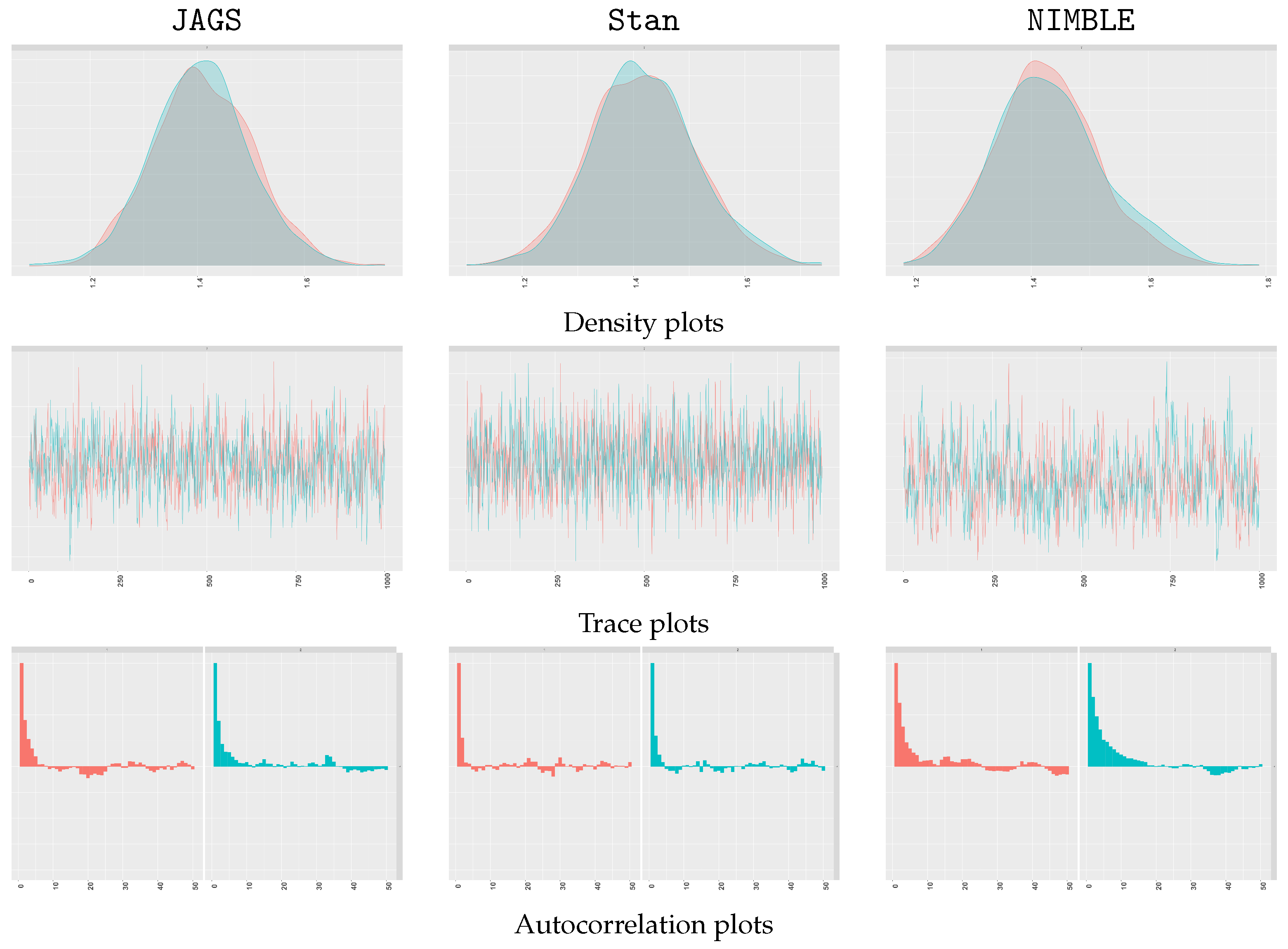
5.1. MCMC Convergence Diagnostics

There are many options for MCMC diagnostics after fitting a Bayesian model through JAGS, Stan, and NIMBLE within the R environment. For example, JAGS users can directly use jagsUI [3] or rjags [4] packages, while Stan users can either work directly within the rstan package [7] or load the bayesplot package [41] that allows visualizing unique diagnostics permitted by HMC and the NUTS algorithm [42,43]. Of note, the recently developed shinystan package[44] is a useful option for analyzing posterior samples. It provides a graphical user interface for interactive plots and tables powered by the Shiny web application framework by R Studio [45]. It works with the output of MCMC programs written in any programming language, and it has extended functionality for the rstan package and the No-U-Turn sampler.

Here, we provide the steps for convergence checking through the ggmcmc [46] package, using $\gamma$ as an example, as shown in Listing 11. The ggmcmc [46] package can be used with any Bayesian software output and provides flexible visualization, bringing the design and implementation of ggplot2 [47] to MCMC diagnostics.

Listing 11: Convergence checking with ggmcmc.

The ggs() function transforms MCMC samples into a data frame tibble object, ready for ggmcmc to use. Note that the ggs() is easily applicable to the Bayesian packages analyzed in this paper. It can take rjags and NIMBLE output (if samplesAsCodaMCMC=T is specified in the sampling function). It can also take the rstan output (after being transformed into mcmc.list through the As.mcmc.list() function in rstan).

We evaluated posterior samples of the model parameters with some visual diagnostics to assess the convergence of each chain. Figure 1 presents the density plots, traceplots, and autocorrelation plots for $\gamma$ using the MCMC samples from JAGS, Stan and NIMBLE. The same sets of diagnostics were run for $\mathsf{\beta }$ and ${\sigma }^2$, and all diagnostics agreed that the model showed good convergence.

5.2. Model Fit Indices: WAIC and LPPD

In the current paper, we worked with a single model specification; hence model comparisons may be unnecessary. For illustration purposes, here we show how model fit indices can be produced, such as Watanabe–Akaike or Widely Applicable Information Criterion (WAIC) [48] and Log Pointwise Predictive Density (LPPD) [49] (Listing 12). WAIC is reportedly preferred over conventional statistics, such as BIC [50] and DIC [51], because of its desirable property of averaging over the posterior distribution, rather than conditioning on a point [49]. An additional advantage is that WAIC produces a stable and positive effective number of parameters (${\widehat{p}}_{waic}$) to evaluate the complexity of the model [52]. LPPD estimates the expected log predictive density for each data point directly, providing a comprehensive evaluation of the model fit to the data regardless of the model’s complexity [49]. These indices are available from rstan and NIMBLE. One can also calculate them using R packages such as loo [53], as used in this paper.

Table 1. WAIC and LPPD for LSIRM model from the three packages.

Index	JAGS	Stan	NIMBLE
WAIC	7166.86	7168.14	7168.63
(${\widehat{p}}_{waic}$)	(672.42)	(674.19)	(675.24)
LPPD	−2911.01	−2909.88	−2909.07

shows WAIC, ${\widehat{p}}_{waic}$ and LPPD from all three packages, which suggests that all these packages produce similar model fit information for the specified LSIRM.

Listing 12: Model fit indices from loo.

5.3. Effective Sample Size, Run Time, and Sampling Efficiency

We evaluated the effective sample size and run time, and, hence, sampling efficiency, of the three packages for LSIRM estimation. All three packages were run on the UCLA hoffman2 cluster computing node that was run on the Intel Xeon Gold 6240 CPU processor, which had a base clock speed of 2.60 GHz and could reach a maximum turbo frequency of 3.90 GHz. The RAM requested for the computing task was fixed at 16 GB.

Table 2. The compilation time and sampling time of the three packages.

Time	JAGS	Stan	NIMBLE
Compilation (min)	6.99	0.67	4.28
Sampling: one core (h)	4.52	3.16	0.87
Sampling: parallel on two cores (h)	1.85	1.04	0.29

Note: ‘one core’ and ‘parallel on two cores’ indicate the cases where the two chains were run separately and simultaneously (using parallel computing), respectively. The time was based on 15,000 iterations and 10,000 burn-in periods, with a thinning interval of 5 for Stan, and 90,000 iterations and 40,000 burn-in periods, with a thinning interval of 50 for JAGS and NIMBLE.

displays the run time for compiling and sampling stages under the chosen iteration/burn-in/thinning conditions of the three packages. All three packages showed satisfactory sampling quality, with Stan performing well with smaller thinning intervals and fewer iterations, while NIMBLE was faster in the sampling stage than the other packages. Note that the compilation time of JAGS included both the model compilation and 1,000 iterations of model adaptation time. As can be seen, parallelization significantly reduced the sampling time for all three packages, compared to the case where a single core was used for sampling the two chains.

The effective sample size (ESS) was a measure of the number of independent draws from the posterior distribution that were equivalent to the actual MCMC draws [54,55]. ESS can be computed with the coda package [15] using the posterior samples of parameters as an input, as shown in Listing 13.

Listing 13: Effective sample size from coda.

Table 3. The ESS and sampling efficiency, ESS/time (s), of the three packages.

	JAGS		Stan		NIMBLE
	ESS	ESS/Time	ESS	ESS/Time	ESS	ESS/Time
$\mathsf{\beta }$	808.81	1.19	1521.01	9.78	688.38	5.26
$\mathsf{\theta }$	1944.10	37.75	1970.61	166.78	1920.58	193.21
$\sigma$	1842.28	0.11	1560.23	0.42	1480.57	0.47
$\gamma$	633.11	0.04	1105.40	0.30	336.79	0.11

Note: For $\mathsf{\beta }$ and $\mathsf{\theta }$, the mean of ESS is reported.

lists the ESS of the LSIRM model parameters from the three packages. While we observed comparable ESS, posterior samples from Stan showed the highest overall ESS, particularly for $\beta$ and $\gamma$ parameters. We further assessed the efficiency of the MCMC estimation in the three packages by calculating the ratio of the ESS to the run time for sampling (ESS/time in seconds) [26,56]. As Table 3 shows, NIMBLE and Stan showed pretty high sampling efficiency. Note that the sample size, model complexity, and choice of priors can significantly impact the run time and sampling efficiency. Users can use the provided tools to evaluate the sampling efficiency for the model of interest with the software of their choice.

6. Estimated Results

6.1. Model Parameters

After convergence and model fit checking, posterior samples can be extracted and further analyzed using various options for post-processing packages in R. Here we demonstrate a universal procedure with coda to summarize the parameters of interest. Listing 14 presents the code for this step.

Listing 14: Extracting information from MCMC chains.

Table 4. The posterior means (Post.m) and 95% credible intervals (CI) of the model parameters of the three packages.

	JAGS			Stan			NIMBLE
	Post.m	95 %CI		Post.m	95 %CI		Post.m	95 %CI
${\beta }_1$	4.01	3.17	5.20	4.05	3.22	5.15	4.03	3.21	5.17
${\beta }_2$	2.54	2.08	3.11	2.55	2.08	3.17	2.56	2.09	3.14
${\beta }_3$	2.33	1.75	3.19	2.34	1.79	3.19	2.36	1.78	3.23
${\beta }_4$	4.00	3.36	4.96	4.03	3.38	4.97	4.06	3.41	4.94
${\beta }_5$	2.55	2.13	3.01	2.57	2.15	3.03	2.58	2.15	3.03
${\beta }_6$	2.59	1.87	3.67	2.59	1.89	3.65	2.60	1.87	3.63
${\beta }_7$	3.67	2.72	4.86	3.67	2.72	4.93	3.61	2.70	4.84
${\beta }_8$	1.60	0.94	2.49	1.60	0.95	2.55	1.57	0.94	2.57
${\beta }_9$	1.27	0.32	2.59	1.30	0.33	2.59	1.28	0.33	2.62
${\beta }_{10}$	3.85	2.89	4.99	3.93	2.97	5.22	3.96	2.98	5.11
${\beta }_{11}$	1.76	1.18	2.63	1.79	1.22	2.60	1.79	1.20	2.70
${\beta }_{12}$	2.02	1.10	3.43	2.03	1.05	3.37	2.01	1.03	3.27
${\beta }_{13}$	3.75	3.00	4.85	3.70	2.96	4.80	3.71	3.00	4.74
${\beta }_{14}$	2.28	1.84	2.84	2.27	1.83	2.77	2.28	1.82	2.81
${\beta }_{15}$	1.12	0.60	1.81	1.12	0.58	1.87	1.12	0.59	1.88
${\beta }_{16}$	3.40	2.66	4.46	3.34	2.63	4.34	3.34	2.65	4.41
${\beta }_{17}$	1.85	1.37	2.43	1.86	1.39	2.44	1.87	1.39	2.50
${\beta }_{18}$	0.51	−0.09	1.26	0.53	−0.06	1.31	0.53	−0.06	1.40
${\beta }_{19}$	1.96	1.36	2.94	1.92	1.34	2.80	1.91	1.33	2.84
${\beta }_{20}$	0.32	−0.21	1.03	0.31	−0.20	0.97	0.30	−0.21	1.02
${\beta }_{21}$	−0.72	−1.68	0.77	−0.69	−1.67	0.84	−0.71	−1.71	0.75
${\beta }_{22}$	3.85	2.90	5.03	3.83	2.88	5.08	3.86	2.89	5.15
${\beta }_{23}$	2.45	1.61	3.58	2.46	1.59	3.69	2.47	1.59	3.71
${\beta }_{24}$	0.63	−0.29	1.96	0.66	−0.27	2.09	0.61	−0.30	1.86
${\sigma }^2$	2.42	1.88	3.02	2.41	1.86	3.04	2.40	1.89	3.04
$\gamma$	1.41	1.24	1.59	1.42	1.24	1.62	1.43	1.26	1.63

lists the posterior means and the lower and upper bounds of 95% credible intervals of the posterior samples of the model parameters. As can be observed, the estimates from the three packages showed high consistency for all investigated parameters.

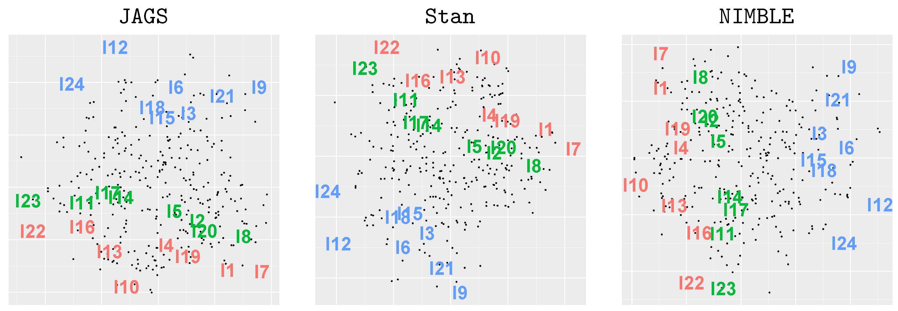
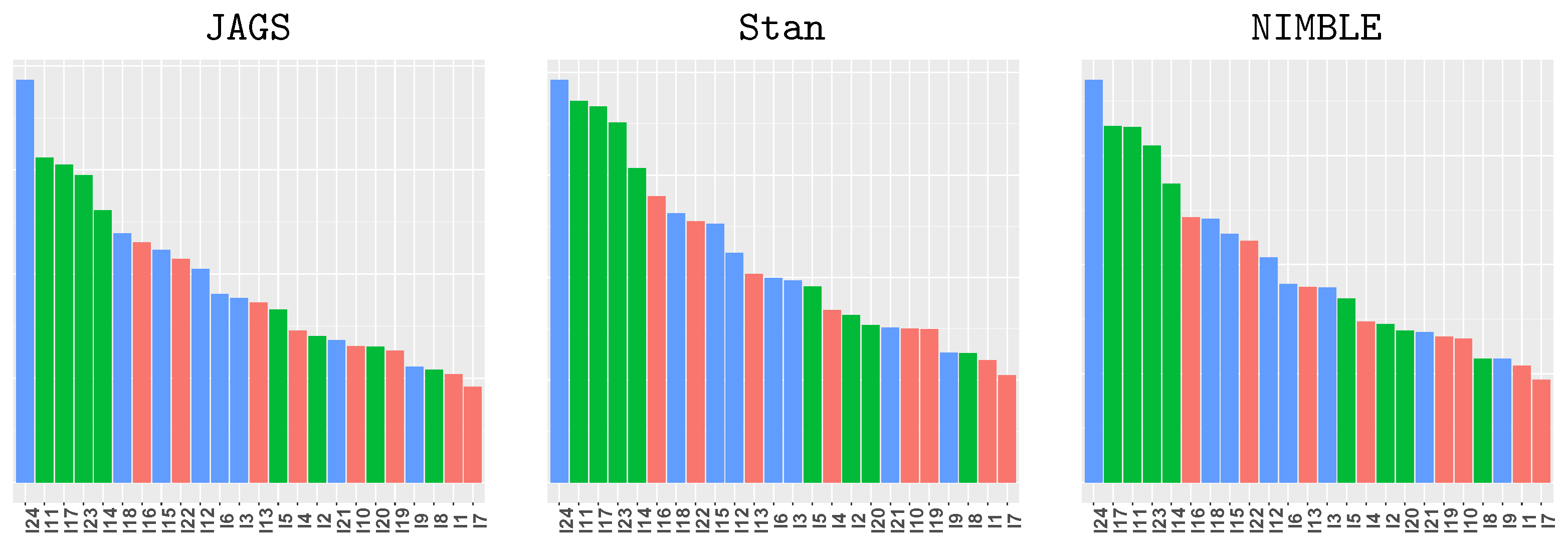
6.2. Interaction Map Visualization

For interaction map visualization, the posterior samples of the person and item latent positions ($\mathbf{z}$ and $\mathbf{w}$) needed to be post-processed to resolve the unidentifiability and match the samples across MCMC iterations, as discussed in Section 2.3. We applied Procrustes matching, as shown in Listing 15. One can use the matched samples to draw the interaction map. Note that zz.samples is a list object that has the dimensions of the number of chains ×, the length of the posterior samples ×, the number of coordinates of $\mathbf{z}$. The number of coordinates equals the product of the sample size (N) and the size of the latent space dimension ($p=2$). JAGS and NIMBLE sort the last dimension of the zz.samples as $z_{11},\dots ,z_{N1},z_{12},\dots ,z_{N2}$, which can be directly processed with the code provided in Listing 15. However, Stan sorts the estimated coordinates as $z_{11},z_{12},\dots ,z_{N1},z_{N2}$; thus, this should be reordered before proceeding with the provided function. The same logic applies to ww.samples. The functions used in Listing 15 can be directly retrieved using the source function with the link provided in Line 13, and can also be obtained from https://anonymous.4open.science/r/LSIRM_Estimation-14EE (accessed on 8 May 2023).

Listing 15: Procrustes matching and visualization of interaction map and strength (inverse distance) plots.

Figure 2 displays the estimated interaction maps from the three packages. In all plots, solid black dots represent respondents, and colored numbers represent items, where Cursing items are in red, Scolding in green, and Shouting in blue. The exact positions of items and respondents were not identical across the three packages, due to the latent positions’ unidenfiability discussed earlier. That said, it can be observed that the overall configuration of the item positions was similar across the three plots. For example, in all plots, the blue item groups were distant from the red and green item groups. There was some separation between the red and green items, although, overall, the two groups (red and green) were close to each other. This indicated strong dependencies (or similarities) among the items within each item group. There were some similarities between Cursing and Scolding items (red and green), which were stronger than similarities between Cursing and Shouting items (red and blue).

As explained earlier, a large distance to an item indicates that the respondent has a lower success probability for the item given her/his overall trait level and the item’s overall difficulty. In other words, a respondent’s distance to an item can be understood as her/his weakness (or lower likelihood) to the item, given her/his overall trait level and the item’s difficulty level. Thus, it can be informative to quantify a person’s distances to the test items to evaluate which items the respondent shows particular strengths or weaknesses (or likelihood or unlikelihood) towards. Figure 3 illustrates Respondent 1’s inverse distances, and, therefore, indicates her/his likelihood of endorsing the 24 verbal aggression items, given the respondent’s overall latent trait level and the item’s difficulty. The items are ordered from the largest to the shortest inverse distances. The three item groups are colored the same way as in Figure 2. Overall, the results were similar across the three packages. To be specific, the three packages gave the same order for the top 5 items. While there were some minor differences, the rank correlations were nearly 1.0 between any package pair, confirming strong similarity in the person–item distances across the three packages.

7. Discussion

In this paper, we presented a practical guide to Bayesian estimation of latent space item response models (LSIRMs), a recent development in IRT, using three popular, free of charge, Bayesian packages, namely, JAGS, Stan, and NIMBLE, run from R through specific packages. With an empirical example, we provided detailed instructions for specifying the model and running the code with each package. We also evaluated model convergence, model fit, sampling quality, and run time. Additionally, we presented the visualization of interaction maps with the three packages.

In regard to the three packages, JAGS is relatively easy to learn and implement, making it suitable for researchers who may be new to Bayesian modeling. With a relatively long history, JAGS boasts an extensive user community that can provide a wide range of support as open-source software. JAGS also supports a wide range of probability distributions, making it a convenient choice for diverse modeling scenarios. Stan, on the other hand, offers an advanced and flexible modeling framework, allowing for efficient estimation of highly complex models involving high-dimensional model parameter space. One key advantage of Stan is its built-in support for parallel computation. NIMBLE strikes a balance between the ease of use of JAGS and the flexibility of Stan. Using a syntax similar to BUGS, NIMBLE allows users to write their own algorithms with the nimbleFunction system, which can be helpful for research and experimentation. In the context of LSIRM estimation, we found that the results were consistent across the three packages with the empirical data under investigation. NIMBLE was somewhat faster than JAGS and Stan, but NIMBLE needed longer chains with larger thinning intervals than Stan. Thus, one may choose a package depending on specific needs and expertise. It is worth noting that, in our illustrative examples, the number of iterations, burning periods, and the length of thinning intervals were chosen to yield posterior samples that had comparable qualities between the three chosen packages. Longer chains were needed for JAGS and NIMBLE to match with Stan’s results in our example. However, different set ups, potentially with a shorter chain, could be considered when comparability between the packages is not of concern.

In closing, we demonstrated, in the current paper, the estimation of LSIRM in an original specification for binary item responses. As LSIRM was introduced as an extension of the Rasch model for conditional dependencies, one may be interested in model selection between LSIRM and the Rasch model. The original paper, [1], addressed the model selection question by applying a spike-and-slab prior to the weight parameter $\gamma$, which can also be implemented in the discussed Bayesian packages. Lastly, to further broaden the applicability of LSIRM, additional research would be needed to show the LSIRM estimation in various other specifications, such as for polytomous data, which is possible due to the flexibility of the Bayesian packages discussed in this paper.

References

1. Jeon, M.; Jin, I.H.; Schweinberger, M.; Baugh, S. Mapping Unobserved Item–Respondent Interactions: A Latent Space Item Response Model with Interaction Map. Psychometrika 2021, 86, 378–403. [Google Scholar] [CrossRef] [PubMed]
2. Rasch, G. On General Laws and the Meaning of Measurement in Psychology. In Proceedings of the Fourth Berkeley Symposium on Mathematical Statistics and Probability, Volume 4: Contributions to Biology and Problems of Health, Oakland, CA, USA, 20 June–30 July 1961; pp. 321–333. [Google Scholar]
3. Ken Kellner, M.M. jagsUI: A Wrapper around ’rjags’ to Streamline ’JAGS’ Analyses; R Package Version 1.5.2; R Core Team: Vienna, Austria, 2021. [Google Scholar]
4. Plummer, M. rjags: Bayesian Graphical Models Using MCMC; R Package Version 4-13; R Core Team: Vienna, Austria, 2022. [Google Scholar]
5. Plummer, M. JAGS: A Program for Analysis of Bayesian Graphical Models Using Gibbs Sampling. In Proceedings of the 3rd International Workshop on Distributed Statistical Computing (DSC 2003), Vienna, Austria, 20–22 March 2003; pp. 1–10. [Google Scholar]
6. Gelman, A.; Lee, D.; Guo, J. Stan: A Probabilistic Programming Language for Bayesian Inference and Optimization. J. Educ. Behav. Stat. 2015, 40, 530–543. [Google Scholar] [CrossRef]
7. Stan Development Team. RStan: The R Interface to Stan; R Package Version 2.21.8; Stan Development Team: Scarborough, OT, USA, 2023. [Google Scholar]
8. De Valpine, P.; Turek, D.; Paciorek, C.; Anderson-Bergman, C.; Temple Lang, D.; Bodik, R. Programming with Models: Writing Statistical Algorithms for General Model Structures with NIMBLE. J. Comput. Graph. Stat. 2017, 26, 403–413. [Google Scholar] [CrossRef]
9. De Valpine, P.; Paciorek, C.; Turek, D.; Michaud, N.; Anderson-Bergman, C.; Obermeyer, F.; Wehrhahn Cortes, C.; Rodrìguez, A.; Temple Lang, D.; Paganin, S. NIMBLE: MCMC, Particle Filtering, and Programmable Hierarchical Modeling; R Package Version 0.12.1; R Foundation for Statistical Computing: Vienna, Austria, 2021. [Google Scholar] [CrossRef]
10. Hoff, P.D.; Raftery, A.E.; Handcock, M.S. Latent Space Approaches to Social Network Analysis. J. Am. Stat. Assoc. 2002, 97, 1090–1098. [Google Scholar] [CrossRef]
11. Shortreed, S.; Handcock, M.S.; Hoff, P. Positional Estimation Within a Latent Space Model for Networks. Methodology 2006, 2, 24–33. [Google Scholar] [CrossRef]
12. Gower, J.C. Generalized Procrustes Analysis. Psychometrika 1975, 40, 33–51. [Google Scholar] [CrossRef]
13. R Core Team. R: A Language and Environment for Statistical Computing; R Foundation for Statistical Computing: Vienna, Austria, 2021. [Google Scholar]
14. Park, J.H.; Cameletti, M.; Pang, X.; Quinn, K.M. CRAN Task View: Bayesian Inference; Comprehensive R Archive Network (CRAN): Vienna, Austria, 2022. [Google Scholar]
15. Plummer, M.; Best, N.; Cowles, K.; Vines, K. CODA: Convergence Diagnosis and Output Analysis for MCMC. R News 2006, 6, 7–11. [Google Scholar]
16. Depaoli, S.; Clifton, J.P.; Cobb, P.R. Just Another Gibbs Sampler(JAGS): Flexible Software for MCMC Implementation. J. Educ. Behav. Stat. 2016, 41, 628–649. [Google Scholar] [CrossRef]
17. Curtis, S.M. BUGS Code for Item Response Theory. J. Stat. Softw. 2010, 36, 1–34. [Google Scholar] [CrossRef]
18. Zhan, P.; Jiao, H.; Man, K.; Wang, L. Using JAGS for Bayesian Cognitive Diagnosis Modeling: A Tutorial. J. Educ. Behav. Stat. 2019, 44, 473–503. [Google Scholar] [CrossRef]
19. Qiu, M. A Tutorial on Bayesian Latent Class Analysis Using JAGS. J. Behav. Data Sci. 2022, 2, 127–155. [Google Scholar] [CrossRef]
20. Merkle, E.C.; Furr, D. Bayesian Comparison of Latent Variable Models: Conditional versus Marginal Likelihoods. Psychometrika 2019, 84, 802–829. [Google Scholar] [CrossRef] [PubMed]
21. Xu, Z. Handling Ignorable and Non-ignorable Missing Data through Bayesian Methods in JAGS. J. Behav. Data Sci. 2022, 2, 99–126. [Google Scholar] [CrossRef]
22. Ciminelli, J.T.; Love, T.; Wu, T.T. Social Network Spatial Model. Spat. Stat. 2019, 29, 129–144. [Google Scholar] [CrossRef]
23. Metropolis, N.; Ulam, S. The Monte Carlo Method. J. Am. Stat. Assoc. 1949, 44, 335–341. [Google Scholar] [CrossRef]
24. Hoffman, S. Zero Benefit: Estimating the Effect of Zero Tolerance Discipline Polices on Racial Disparities in School Discipline. Educ. Policy 2014, 28, 69–95. [Google Scholar] [CrossRef]
25. Neal, D.T.; Wood, W.; Wu, M.; Kurlander, D. The Pull of the Past: When Do Habits Persist Despite Conflict with Motives? Personal. Soc. Psychol. Bull. 2011, 37, 1428–1437. [Google Scholar] [CrossRef] [PubMed]
26. Monnahan, C.C.; Thorson, J.T.; Branch, T.A. Faster Estimation of Bayesian Models in Ecology Using Hamiltonian Monte Carlo. Methods Ecol. Evol. 2017, 8, 339–348. [Google Scholar] [CrossRef]
27. Bølstad, J. How Efficient is Stan Compared to JAGS? Conjugacy, Pooling, Centering, and Posterior Correlations. Playing with Numbers: Notes on Bayesian Statistics. 2019. Available online: https://www.boelstad.net/post/stan_vs_jags_speed/ (accessed on 1 May 2023).
28. Salter-Townshend, M.; McCormick, T.H. Latent Space Models for Multiview Network Data. Ann. Appl. Stat. 2017, 11, 1217. [Google Scholar] [CrossRef]
29. Salter-Townshend, M.; Murphy, T.B. Variational Bayesian Inference for the Latent Position Cluster Model for Network Data. Comput. Stat. Data Anal. 2013, 57, 661–671. [Google Scholar] [CrossRef]
30. Beraha, M.; Falco, D.; Guglielmi, A. JAGS, NIMBLE, Stan: A detailed comparison among Bayesian MCMC software. arXiv 2021, arXiv:2107.09357. [Google Scholar]
31. Paganin, S.; Paciorek, C.J.; Wehrhahn, C.; Rodríguez, A.; Rabe-Hesketh, S.; de Valpine, P. Computational Strategies and Estimation Performance with Bayesian Semiparametric Item Response Theory Models. J. Educ. Behav. Stat. 2023, 48, 147–188. [Google Scholar] [CrossRef]
32. Wang, W.; Kingston, N. Using Bayesian Nonparametric Item Response Function Estimation to Check Parametric Model Fit. Appl. Psychol. Meas. 2020, 44, 331–345. [Google Scholar] [CrossRef] [PubMed]
33. Ma, Z.; Chen, G. Bayesian Semiparametric Latent Variable Model with DP Prior for Joint Analysis: Implementation with NIMBLE. Stat. Model. 2020, 20, 71–95. [Google Scholar] [CrossRef]
34. Gelman, A.; Simpson, D.; Betancourt, M. The prior can often only be understood in the context of the likelihood. Entropy 2017, 19, 555. [Google Scholar] [CrossRef]
35. Depaoli, S.; Winter, S.D.; Visser, M. The importance of prior sensitivity analysis in Bayesian statistics: Demonstrations using an interactive Shiny App. Front. Psychol. 2020, 11, 608045. [Google Scholar] [CrossRef]
36. Zitzmann, S.; Lüdtke, O.; Robitzsch, A.; Hecht, M. On the performance of Bayesian approaches in small samples: A comment on Smid, McNeish, Miocevic, and van de Schoot (2020). Struct. Equ. Model. Multidiscip. J. 2021, 28, 40–50. [Google Scholar] [CrossRef]
37. Smid, S.C.; McNeish, D.; Miočević, M.; van de Schoot, R. Bayesian versus frequentist estimation for structural equation models in small sample contexts: A systematic review. Struct. Equ. Model. Multidiscip. J. 2020, 27, 131–161. [Google Scholar] [CrossRef]
38. De Boeck, P.; Wilson, M. (Eds.) Explanatory Item Response Models: A Generalized Linear and Nonlinear Approach; Springer: New York, NY, USA, 2004; pp. 7–10. [Google Scholar] [CrossRef]
39. Magis, D.; Beland, S.; Tuerlinckx, F.; De Boeck, P. A General Framework and an R Package for the Detection of Dichotomous Differential Item Functioning. Behav. Res. Methods 2010, 42, 847–862. [Google Scholar] [CrossRef]
40. Jeon, M.; Rijmen, F. A Modular Approach for Item Response Theory Modeling with the R Package Flirt. Behav. Res. Methods 2016, 48, 742–755. [Google Scholar] [CrossRef]
41. Gabry, J.; Simpson, D.; Vehtari, A.; Betancourt, M.; Gelman, A. Visualization in Bayesian Workflow. J. R. Stat. Soc. A 2019, 182, 389–402. [Google Scholar] [CrossRef]
42. Betancourt, M. A conceptual introduction to Hamiltonian Monte Carlo. arXiv 2017, arXiv:1701.02434. [Google Scholar]
43. Betancourt, M.; Girolami, M. Hamiltonian Monte Carlo for Hierarchical Models. Curr. Trends Bayesian Methodol. Appl. 2015, 79, 2–4. [Google Scholar] [CrossRef]
44. Gabry, J.; Veen, D. Shinystan: Interactive Visual and Numerical Diagnostics and Posterior Analysis for Bayesian Models; R Package Version 2.6.0; R Foundation for Statistical Computing: Vienna, Austria, 2022. [Google Scholar]
45. RStudio Team. RStudio: Integrated Development for R; RStudio, PBC: Boston, MA, USA, 2020. [Google Scholar]
46. Fernández-i-Marín, X. ggmcmc: Analysis of MCMC Samples and Bayesian Inference. J. Stat. Softw. 2016, 70, 1–20. [Google Scholar] [CrossRef]
47. Valero-Mora, P.M. ggplot2: Elegant Graphics for Data Analysis. J. Stat. Softw. Book Rev. 2010, 35, 1–3. [Google Scholar] [CrossRef]
48. Watanabe, S. Asymptotic Equivalence of Bayes Cross Validation and Widely Applicable Information Criterion in Singular Learning Theory. J. Mach. Learn. Res. 2010, 11, 3571–3594. [Google Scholar] [CrossRef]
49. Gelman, A.; Hwang, J.; Vehtari, A. Understanding Predictive Information Criteria for Bayesian Models. Stat. Comput. 2014, 24, 997–1016. [Google Scholar] [CrossRef]
50. Schwarz, G. Estimating the Dimension of a Model. Ann. Stat. 1978, 6, 461–464. [Google Scholar] [CrossRef]
51. Spiegelhalter, D.J.; Best, N.G.; Carlin, B.P.; van der Linde, A. Bayesian Measures of Model Complexity and Fit. J. R. Stat. Soc. Ser. B (Stat. Methodol.) 2002, 64, 583–639. [Google Scholar] [CrossRef]
52. Vehtari, A.; Gelman, A.; Gabry, J. Practical Bayesian Model Evaluation Using Leave-One-Out Cross-Validation and WAIC. Stat. Comput. 2017, 27, 1413–1432. [Google Scholar] [CrossRef]
53. Vehtari, A.; Gabry, J.; Magnusson, M.; Yao, Y.; Bürkner, P.C.; Paananen, T.; Gelman, A. loo: Efficient Leave-One-Out Cross-Validation and WAIC for Bayesian Models; R Package Version 2.5.1; R Foundation for Statistical Computing: Vienna, Austria, 2022. [Google Scholar]
54. Gelman, A.; Carlin, J.B.; Stern, H.S.; Dunson, D.B.; Vehtari, A.; Rubin, D.B. Bayesian Data Analysis; CRC Press: Boca Raton, FL, USA, 2013; pp. 286–287. [Google Scholar] [CrossRef]
55. Zitzmann, S.; Hecht, M. Going beyond convergence in Bayesian estimation: Why precision matters too and how to assess it. Struct. Equ. Model. Multidiscip. J. 2019, 26, 646–661. [Google Scholar] [CrossRef]
56. Hecht, M.; Weirich, S.; Zitzmann, S. Comparing the MCMC Efficiency of JAGS and Stan for the Multi-Level Intercept-Only Model in the Covariance- and Mean-Based and Classic Parametrization. Psych 2021, 3, 751–779. [Google Scholar] [CrossRef]
Figure 1. Visual diagnostics of γ from the three packages. The first, second, and third rows show density plots, trace plots, and autocorrelation plots, respectively. The three columns indicate JAGS, Stan, and NIMBLE results, respectively. Note that the first MCMC chain is displayed in red and the second MCMC chain in light blue.
Psych 05 00027 g001
Figure 2. Estimated interaction maps of the matched latent positions from the three packages. In all plots, solid black dots represent respondents, and colored numbers represent items, where Cursing items are in red, Scolding in green, and Shouting in blue.
Psych 05 00027 g002
Figure 3. Respondent 1’s inverse distances to the 24 verbal aggression items estimated from the three packages. The height of the bars indicates respondent 1’s likelihood of endorsing the item, given her/his overall trait level and the item’s difficulty. The items are ordered from the highest to lowest endorsement likelihood for Respondent 1. The coloring of the bars is based on item types, where Cursing items are in red, Scolding in green and Shouting in blue.
Psych 05 00027 g003