
Applications and Extensions of Metric Stability Analysis

Department of Psychology, Fordham University, Bronx, NY 10458, USA
Psych 2023, 5(2), 376-385; https://doi.org/10.3390/psych5020025
Submission received: 31 March 2023
/
Revised: 26 April 2023
/
Accepted: 28 April 2023
/
Published: 4 May 2023
(This article belongs to the Special Issue Computational Aspects and Software in Psychometrics II)
Abstract
:Item response theory models and applications are affected by many sources of variability, including errors associated with item parameter estimation. Metric stability analysis (MSA) is one method to evaluate the effects of item parameter standard errors that quantifies how well a model determines the latent trait metric. This paper describes how to evaluate MSA in dichotomous and polytomous data and describes a Bayesian implementation of MSA that does not require a positive definite variance–covariance matrix among item parameters. MSA analyses are illustrated in the context of an oral-health-related quality of life measure administered before and after prosthodontic treatment. The R code to implement the methods described in this paper is provided.
1. Introduction
When using item response theory (IRT) models to score examinees, there are several factors that may cause score estimates to vary. Jones, Wainer, and Kaplan [1] (see also [2]) enumerated four sources of score variability:
- Variability associated with the inherently probabilistic nature of item response models, captured by the model-implied information and standard errors of trait estimates.
- Variability associated with a particular trait estimation method.
- Variability associated with item parameter estimate.
- Variability associated with imperfect match of a model to data.
Uncertainty associated with the first and second sources is quantified by the standard errors of item parameter estimates. Uncertainty associated with the third and fourth sources—errors in item parameters and errors in model selection—are often ignored when using IRT-based person-scoring algorithms, though several estimation methods that account for these errors have been proposed [3,4,5,6,7,8,9]. The impact of the third and fourth sources on score estimates is not ignorable. Neglecting to account for these sources of variability can lead to inaccurate estimates of latent trait scores and their standard errors [8] and negatively affect the results of other IRT-based procedures [10,11,12,13]. In addition, there is evidence that the linear nature of a model (i.e., the location and units of the latent trait scale) is not always well-determined when item parameters are estimated with error [14]. Therefore, it is pertinent to routinely evaluate how well the latent trait metric is determined for a given fitted model.
Understanding and properly accounting for errors associated with item parameter uncertainty ought to be a routine part of model evaluation. However, relatively few methods exist to evaluate the impact of these factors. These methods include inspecting the parameter standard errors, which can be difficult to synthesize, or calculating confidence envelopes [15,16] around the predicted item or test response curves. Although confidence envelopes are a useful visual tool, they only consider variability with respect to a fixed metric (i.e., they cannot reflect nonlinear distortions of the latent trait metric across sets of plausible parameters [14]). In addition, it is unclear how to use the information provided by confidence envelopes to quantitatively assess which regions of the latent trait metric are well-determined by the model.
Feuerstahler [14] proposed metric stability analysis (MSA) as a way to express item parameter standard errors in terms of their effects on the latent trait metric itself. The aims of the current study are to extend metric stability analysis (MSA) to polytomous item response models and to develop Bayesian methods for MSA that do not require direct estimation of item parameter standard errors. These Bayesian methods are especially useful for evaluating a complex model for which it is difficult or impossible to obtain a positive definite matrix of item parameter variances and covariances. First, metric stability as it was originally proposed [14] will be described along with its implementation using the mirt [17] package for R [18]. Second, a fully Bayesian approach to MSA will be described and exemplified using the brms [19] package for R. Third, we will apply MSA to the analysis of longitudinal patient-reported outcomes data to demonstrate how MSA provides useful information to supplement other model evaluation tools.
1.1. Metric Stability Analysis Using Multiple Imputation
The approach to MSA proposed by Feuerstahler [14] follows from a geometrical definition of the IRT latent trait. Specifically, for a test composed of I items each with response categories, the latent trait metric is a vector-valued function composed of the set of response probabilities for categories . Probabilities associated with the lowest response category, 0, are excluded from this definition because category response probabilities must sum to 1 for any given item. For illustration, consider the two-parameter logistic item response model (2PL) for which
where and reflect item-specific discrimination and intercept parameters, and is the latent trait parameter. Suppose that three items are fit to the 2PL such that = 0.75, = 1, = 1.25, , = 0.5, and . Each value is associated with a triplet of predicted response probabilities, for example, : and : . In this way, the IRT latent trait metric can be defined entirely in terms of these sets of associated response probabilities, which will trace a trajectory in multidimensional space. For more information, see [14,20].
An important feature of the geometrical definition of the latent trait is that it is invariant to the scaling of . In other words, the vectors of associated probilities will be identical for every linear or (monotonic) nonlinear transformation of , as these transformed models make identical predictions [21]. This invariant latent trait definition also makes it possible to compare the similarity of predictions made by different models based on the same data and to understand how uncertainty in item parameter estimates affects the precision of predicted response probabilities. The latter is the goal of MSA. Specifically, MSA characterizes metric uncertainty in terms of variability in the vector of predicted response probabilities.
MSA can be evaluated as follows. For a fitted item response model with point estimates of the item parameters and variance–covariance among item parameter estimates , draw M multiply imputed (MI [9]) samples from a multivariate normal distribution with mean and covariance . Then, select Q values at which to evaluate metric stability. Let f be the vector of n predicted probabilities to all items on a test, excluding the lowest response category for each item. The Euclidean distance between and any point r on the trajectory implied by , equals
Then, metric stability can be quantified for each value of and by minimizing as a function of :
In other words, Equation (3) finds the Euclidean distance between point q on the trajectory implied by and the nearest location on the trajectory implied by . The more similar the MI trajectories are to the trajectory based on point estimates, the smaller the values of , and can be interpreted as the root mean squared difference between a point on the point-estimated trajectory and the nearest point on the trajectory implied by MI draw m. Metric stability can be evaluated as a function of at each q value by taking medians or other quantiles of across the M values. By evaluating metric stability at each value, researchers can understand the magnitude of metric variability as well as the regions of the latent trait metric that are well-determined by the fitted model.
1.2. Bayesian Metric Stability Analysis
There are several potential limitations to the MI-based MSA approach described above. First, this approach relies on the assumption of available, accurate, and normally distributed standard errors of item parameters. However, it can be difficult to obtain a positive definite , especially for complex models [22]. A second limitation is that this method relies on numerical optimization computed separately for each point. That is, optimization-based MSA does not guarantee that the values that minimize Equation (3) increase monotonically with within any given iteration m.
Two new strategies to assess metric stability are available when jointly estimating item and person parameters through Bayesian Markov chain Monte Carlo (MCMC) [23]. MCMC estimation results in a large number of draws from the joint posterior distribution of and . In the first proposed strategy, the posterior draws of item parameters can serve the same role as the M multiple imputation draws and the posterior mean of each parameter can serve as . This optimization-based strategy shares the properties listed in the previous section, except that the posterior samples are always available and do not need to be sampled from a multivariate normal distribution. Although this strategy assumes that the MCMC model has converged, it avoids the common problem of unavailable item parameter standard errors. Specifically, many IRT model estimation methods other than MCMC compute standard errors by inverting a parameter information matrix. Inversion is unstable or impossible under the common scenario that the information matrix is (nearly) singular. Even for estimation algorithms that do not involve inverting an information matrix such as the Metropolis–Hasings Robbins–Monro (MH-RM) algorithm [24], the resulting variance–covariance matrix may not be positive definite. These problems in obtaining item parameter standard errors were repeatedly encountered when using the mirt package for the analyses described in this paper.
A second, quantile-based, strategy based on MCMC calculates metric stability based on quantiles of the estimated distribution at each draw m rather than finding the nearest trajectory point. This approach relies on a monotonically ordered scale such that the predicted response probabilities associated with quantiles of are invariant to transformations of . To implement the quantile-based MSA measure, evaluate Equation (2) for each posterior draw m, setting to be the posterior mean at each quantile, and setting equal to the estimate that exists at the qth quantile of iteration m. Then, medians or other quantiles of the resulting values, which function in the same way as , can be used to evaluate metric stability in a similar way as the optimization-based strategy. Note that this quantile-based strategy is only available when joint estimates both of the item and person parameters are available, as with MCMC estimation because it uses observed quantiles of throughout the posterior distribution space. In addition to not requiring a positive definite variance–covariance matrix, this method involves no optimization and will guarantee a continuous trajectory within each iteration.
2. Methods
In the remainder of this paper, we illustrate MSA in an empirical application and provide R code so that researchers can apply these methods to their own models and data. First, metric stability is analyzed in several ways in both mirt and brms. Second, we apply MSA to longitudinal models and demonstrate that despite the added model complexity, the metric becomes more stable when item parameters are informed by information at multiple time points.
2.1. Data for Illustration
In this paper, we use data from the Oral Health Impact Profile-German version (OHIP-G) [25]. These data were previously analyzed in the context of identifying meaningful change score effect sizes [26] and include responses from 224 adults before and after receiving prosthodontic treatment (fixed prosthodontics, removable partial dentures, or complete dentures). Further information about this sample is provided elsewhere [26]. The OHIP-G includes 49 items for which patients self-report how often in the past month they experienced various oral-health-related problems on a five-point Likert scale with labels 0 = ‘never’, 1 = ‘hardly ever’, 2 = ‘occasionally’, 3 = ‘fairly often’, and 4 = ‘very often’. Patients responded to this survey at two baseline appointments (separated by 1 to 2 weeks) and again after prosthodontic treatment. For the purpose of the current study, we focus on 5 items that belong to a previously proposed short form known as the OHIP-5 [27]. To simplify analyses, the full sample of respondents was restricted to the respondents who provided complete OHIP-5 data at each time point. In addition, very few responses were in the upper categories for each item, and several categories have zero frequencies for some time points, especially at follow-up. As such, we rescored responses so that data are observed in consecutive integers within each item and time point. We also analyzed a dichotomized data set that combined responses to categories 1 through 4 for each item. The full text of these items is available elsewhere [28], and Table 1 presents shortened item content and summary statistics at each time point for the reduced data. As expected, mean responses are generally lower at follow-up than at either baseline assessment, reflecting that the treatment may have resulted in an improved quality of life. At all time points, responses are highly positively skewed, indicating that many patients seeking prosthodontic treatment have high oral-health-related quality of life in some respects, even before treatment.
As expected, two-tailed paired-samples t-tests comparing sum scores (before any rescoring) for the two baseline measures were not statistically significant at (t(184) = 1.09, p = 0.28). Both paired-samples t-tests comparing baseline scores to post-treatment scores indicated a significant decrease in reported problems (baseline 1 vs. follow-up: ; baseline 2 vs. follow-up: ).
2.2. MSA at Each Time Point
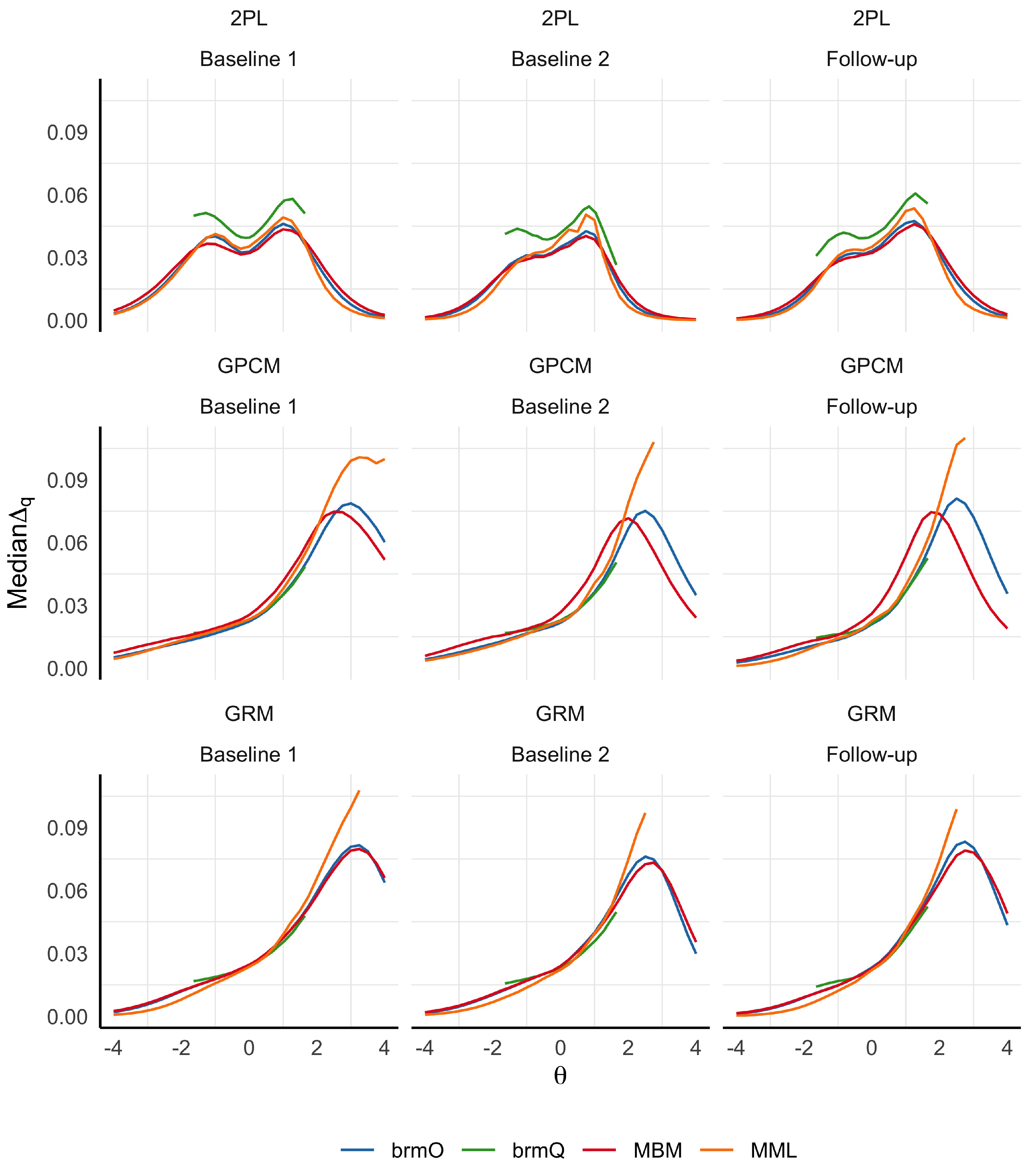
Next, metric stability was evaluated in several ways separately for each time point. A total of three item response models were considered: the graded response model (GRM [30] and the generalized partial credit model (GPCM [31]) for the rescored polytomous data, and the 2PL for the dichotomized data. Models were fit in either the mirt [17] or brms [19] packages for R [18]. For each time point and for each of the 2PL, GRM, and GPCM, MSA was evaluated in four ways: in mirt [17] fit with both marginal maximum likelihood (MML) and marginal Bayes model (MBM) estimation, and in brms [19] using both optimization-based and quantile-based MSA.
The exact specification of the GRM and GPCM varies across software packages used in this study. These differences are notable because the parameters for which standard errors are calculated vary across software. For the GRM implemented in mirt, the probability of a response in category or greater equals
whereas the same model in brms uses
with the opposite sign for the parameters and defining . In Equation (4), the parameters must be strictly decreasing whereas in Equation (5) they must be strictly increasing. The GPCM in mirt gives the probability of a response in a specific category as
whereas the same model in brms uses
Regardless of these differences in parameterization, all Bayesian models were fit with the priors and , and the same priors were used for all parameters and all parameterizations. Models fit in mirt used package defaults for item parameter and standard error estimation, except as indicated. Models fit in brms were run using 4 parallel chains of 2000 iterations each, with the first 1000 iterations of each chain discarded as burn-in for a total of samples used for MSA.
For the models estimated in mirt, MI samples were generated from multivariate normal distributions. For MSA analyzed through numerical optimization, stability was estimated at in intervals of 0.25. For MSA analyzed with quantiles, quantiles from 0.05 to 0.95 were used in intervals of 0.05. For all MSA analyses reported in this paper, q-specific medians of across the M values were used as the measures of metric stability. For visualization, we plotted quantile-based results against the associated quantiles of the standard normal distribution.
R code to reproduce these analyses on a simulated data set based on the Baseline 1 model is included in the Supplementary Materials of this paper.
2.3. Longitudinal Analyses
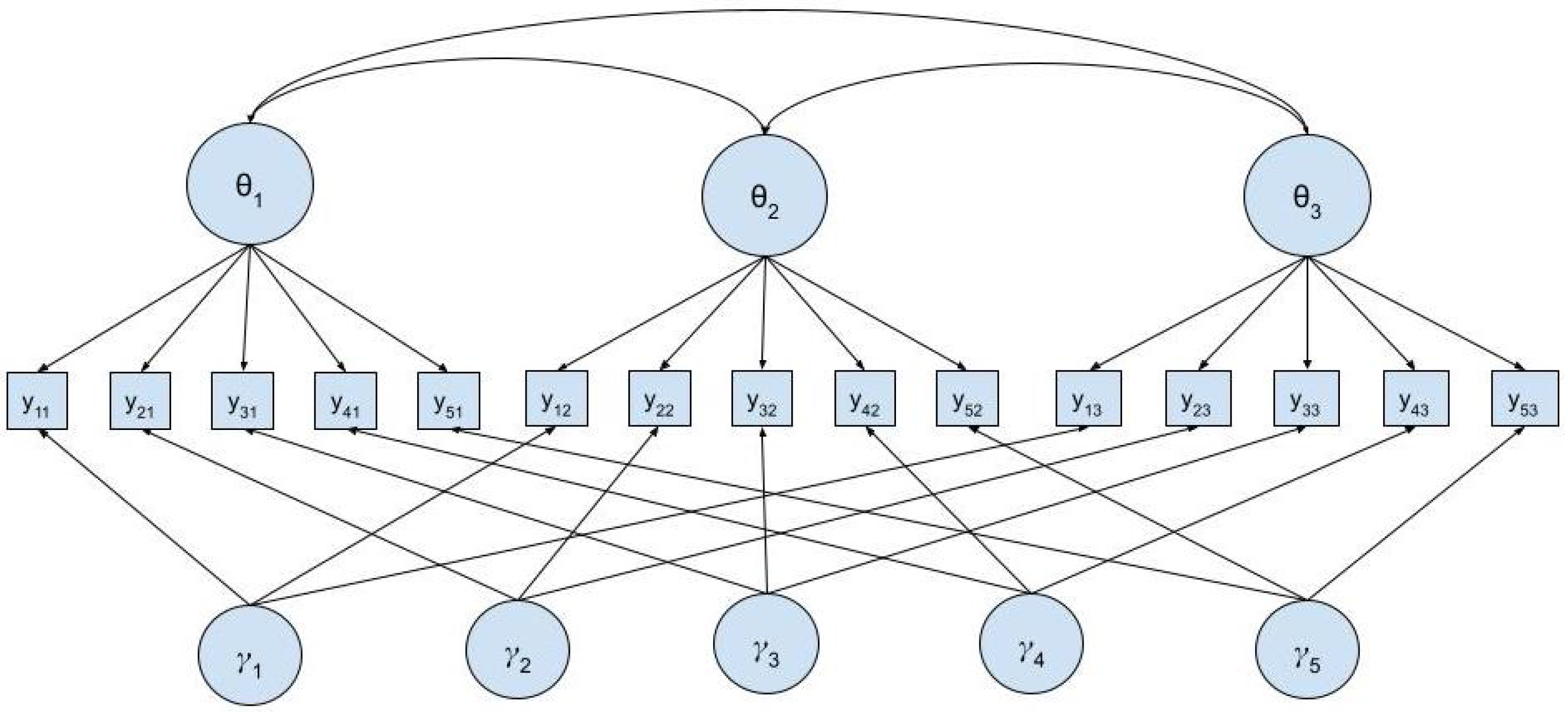
Next, we fit data from multiple time points to Cai’s two-tier model [32] to account for the longitudinal nature of these data. This model is a special case of a bifactor model that includes a primary dimension for each time point and specific factors for each item that capture the residual covariance among items expected from the use of longitudinal data. A path diagram of this model applied to five items and three time points is given in Figure 1. In this model, primary dimensions , , and represent the latent trait scores at baseline 1, baseline 2, and follow-up. Specific dimensions capture the item covariances associated with administering the same items multiple times to the same patients. This model allows for correlations among the three primary dimensions, but the specific dimensions are uncorrelated with the primary dimensions and with each other. In addition, for each item i, all item parameters (primary factor discriminations, specific factor discriminations, and intercepts) are constrained to equal the same values across time points.
In this section, three 2PL models were fit to the dichotomized OHIP-5 data: a unidimensional model using only baseline 1 data, a two-tier model using both baseline 1 and baseline 2 data, and a two-tier model using baseline 1, baseline 2, and follow-up data. All models were fit using mirt and the MH-RM algorithm. In exploring variations of this model with the OHIP-G data, we often found non-positive definite variance–covariance matrices of item parameters, some of which included negative diagonal elements. Because a positive definite parameter covariance matrix is needed to draw MI samples from a multivariate normal distribution, the following specifications were made for these analyses. First, Bayesian priors were used to stabilize estimation with for primary dimensions, for specific dimensions, and . The resulting covariance matrices were still not positive definite for the two longitudinal models, so only covariances among the primary dimension and were used to draw MI samples. For all models, metric stability was calculated based on the primary dimension and item parameters alone, ignoring the effects of the specific dimensions.
3. Results
3.1. Metric Stability at Each Time Point
Metric stability for each model and method is visualized in Figure 2. Although results are presented in different panels for different models, it is theoretically appropriate to directly compare results from different models based on the same data (here, at the same time point), so long as the underlying metric is the same. Note that lower values of median indicate less variability in predicted probabilities. Although the choice of an upper cutoff for “stable enough” is subjective, Feuerstahler [14] recommended an upper bound of 0.02 for median values. Most regions for all models in this example do not meet this criterion, largely because of the relatively small sample size used to fit the IRT models.
For most panels in Figure 2, different measures of metric stability yield similar results, suggesting that any of these methods is appropriate to evaluate MSA. However, some within-panel differences appear to be due to differences in model specification. For example, for the GPCM and GRM, MML yields increasing instability at high values, whereas the prior used in the Bayesian models decreases the magnitude of this effect. Minor differences in instability between MBM and MML are visible for nearly all models. Finally, the quantile-based method appears systematically higher than the optimization-based methods for the 2PL. This may be because the optimization-based methods explicitly seek the nearest points in the posterior space; however, it is not clear why this phenomenon does not occur for the GPCM or GRM.
3.2. Longitudinal Measurement Stability
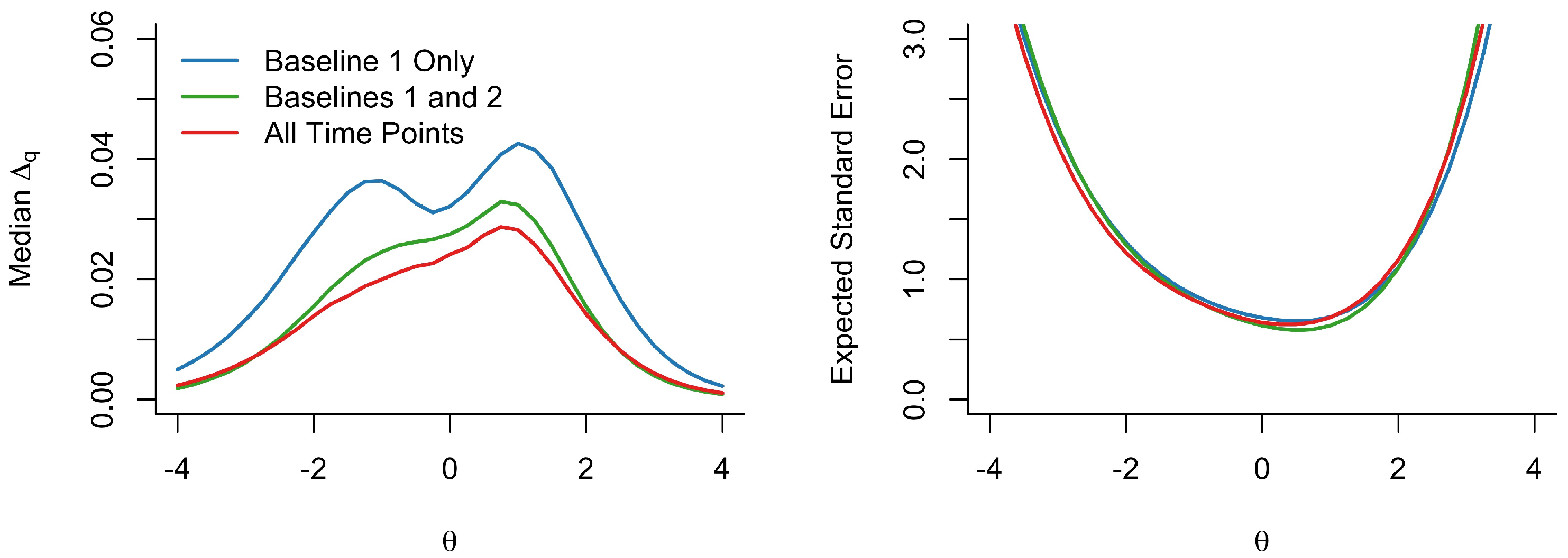
Figure 3 shows results based on the models built on one, two, and three time points. In the left-hand panel, our metric stability measure shows increased stability (lower median ) at all values for models built on more time points. The model built on three time points yields median values less than 0.03, though median is only less than the 0.02 cutoff for and . The right-hand panel shows the expected standard error functions (i.e., the inverse square root of test information in the direction of the primary dimension). The expected standard errors are approximately equal across the three fitted models, indicating that the expected variability due to probabilistic responding and trait estimation is unaffected by the use of a single-time-point or longitudinal model.
Note that the regions of that MSA indicates as more stable tend to be those at extreme values, which happen to be regions associated with higher standard errors. This phenomenon tends to occur because predicted response probabilities are less variable at extreme values (i.e., where all response probabilities tend toward 0 or 1), but these regions also tend to provide low information because the predicted item response curves are relatively flat at extreme values. That these two measures seemingly disagree about the reliability of highlights that MSA and information reflect different types of errors in IRT models. Therefore, we recommend that researchers analyze both simultaneously, seeking a model that yields both low values and low expected standard errors at the regions intended to be measured well by the test.
4. Discussion
The primary contributions of this paper are the extensions of metric stability analysis (MSA [14]) to polytomous data, the Bayesian MCMC implementation of MSA, and the presentation of R code that researchers can adapt to investigate MSA in their own data. Through an empirical illustration, this paper demonstrates that the different strategies for investigating MSA usually yield comparable values, though differences in model specification and use of informative priors can affect the regions of that are more and less stable. The fact that different methods tend to yield comparable results, particularly for similar model specifications, suggests that only one type of MSA needs to be used in any real data analysis, so long as it corresponds to the model specification used in other analyses of the same data.
The Bayesian MCMC methods described in this paper are particularly promising alternatives to the MI approach described earlier [14]. This is because Bayesian MCMC directly samples from the posterior distribution of item parameters rather than drawing MI samples from a multivariate normal distribution. Such use of MI is limited because it requires a positive definite matrix variance–covariance matrix among item parameters, which can be difficult or impossible to attain for complex multidimensional or longitudinal models [22].
MSA as described in this paper is currently limited to reflective measurement models for categorical data and continuous latent traits (i.e., item response models). Although several empirical and simulation-based applications of MSA were provided in previous work [14], future work should expand the variety of applications of this method. In addition, future work may extend the MSA strategy to other measurement models such as cognitive diagnostic models, factor analysis, or formative models.
5. Conclusions
Understanding the consequences of item parameter estimation error ought to be a routine part of item response model evaluation. MSA is an improvement on previous methods with similar goals [16,33] in that it provides both visual and quantitative information and allows for nonlinear relationships between different models. In summary, we hope that the developments and R code described in this paper will help facilitate the more routine use of MSA.
Supplementary Materials
The following supporting information can be downloaded at: https://www.mdpi.com/article/10.3390/psych5020025/s1.
Funding
This research received no external funding.
Institutional Review Board Statement
Not applicable.
Data Availability Statement
Simulated data similar to that analyzed in this paper are available in the Supplementary Materials, along with R code to implement the methods described in this paper.
Acknowledgments
Data analyzed in this paper were generously provided by Mike John.
Conflicts of Interest
The author declares no conflict of interest.
Abbreviations
The following abbreviations are used in this manuscript:
| 2PL | Two-parameter logistic item response model |
| GPCM | Generalized partial credit model |
| GRM | Graded response model |
| IRT | Item response theory |
| MBM | Marginal Bayes model estimation |
| MCMC | Markov Chain Monte Carlo |
| MH-RM | Metropolis–Hastings Robbins–Monro |
| MI | Multiple imputations |
| MML | Marginal maximum likelihood estimation |
| MSA | Metric stability analysis |
| OHIP-5 | Five-item short form of the Oral Health Impact Profile |
| OHIP-G | Oral Health Impact Profile, German version |
References
- Jones, D.H.; Wainer, H.; Kaplan, B. Estimating ability with three item response models when the models are wrong and their parameters are inaccurate. ETS Res. Rep. Ser. 1984, 1984, i-50. [Google Scholar] [CrossRef]
- Feuerstahler, L.M. Sources of error in IRT trait estimation. Appl. Psychol. Meas. 2018, 42, 359–375. [Google Scholar] [CrossRef] [PubMed]
- Cheng, Y.; Yuan, K.H. The impact of fallible item parameter estimates on latent trait recovery. Psychometrika 2010, 75, 280–291. [Google Scholar] [CrossRef] [PubMed]
- Hoshino, T.; Shigemasu, K. Standard errors of estimated latent variable scores with estimated structural parameters. Appl. Psychol. Meas. 2008, 32, 181–189. [Google Scholar] [CrossRef]
- Liu, Y.; Yang, J.S. Bootstrap-calibrated interval estimates for latent variable scores in item response theory. Psychometrika 2018, 83, 333–354. [Google Scholar] [CrossRef]
- Mislevy, R.J.; Wingersky, M.S.; Sheehan, K.M. Dealing with uncertainty about item parameters: Expected response functions. ETS Res. Rep. Ser. 1994, 1994, i-20. [Google Scholar]
- Patton, J.M.; Cheng, Y.; Yuan, K.H.; Diao, Q. Bootstrap standard errors for maximum likelihood ability estimates when item parameters are unknown. Educ. Psychol. Meas. 2014, 74, 697–712. [Google Scholar] [CrossRef]
- Tsutakawa, R.K.; Johnson, J.C. The effect of uncertainty of item parameter estimation on ability estimates. Psychometrika 1990, 55, 371–390. [Google Scholar] [CrossRef]
- Yang, J.S.; Hansen, M.; Cai, L. Characterizing sources of uncertainty in item response theory scale scores. Educ. Psychol. Meas. 2012, 72, 264–290. [Google Scholar] [CrossRef]
- Baldwin, P. A strategy for developing a common metric in item response theory when parameter posterior distributions are known. J. Educ. Meas. 2011, 48, 1–11. [Google Scholar] [CrossRef]
- Pashley, P.J. Graphical IRT-based DIF analyses. ETS Res. Rep. Ser. 1992, 1992, i-20. [Google Scholar] [CrossRef]
- Scrams, D.J.; McLeod, L.D. An expected response function approach to graphical differential item functioning. J. Educ. Meas. 2000, 37, 263–280. [Google Scholar] [CrossRef]
- Sheehan, K.M.; Mislevy, R.J. Some consequences of the uncertainty in IRT linking procedures. ETS Res. Rep. Ser. 1988, 1988, i-40. [Google Scholar] [CrossRef]
- Feuerstahler, L.M. Metric stability in item response models. Multivar. Behav. Res. 2022, 57, 94–111. [Google Scholar] [CrossRef] [PubMed]
- Thissen, D.; Wainer, H. Confidence Envelopes for Monotonic Functions: Principles, Derivations, and Examples; Technical Report; Mcfann Gray and Associates Inc.: San Antonio, TX, USA, 1983. [Google Scholar]
- Thissen, D.; Wainer, H. Confidence envelopes for item response theory. J. Educ. Stat. 1990, 15, 113–128. [Google Scholar] [CrossRef]
- Chalmers, R.P. mirt: A multidimensional item response theory package for the R environment. J. Stat. Softw. 2012, 48, 1–29. [Google Scholar] [CrossRef]
- R Core Team. R: A Language and Environment for Statistical Computing; R Foundation for Statistical Computing: Vienna, Austria, 2023. [Google Scholar]
- Bürkner, P.C. brms: An R package for Bayesian multilevel models using Stan. J. Stat. Softw. 2017, 80, 1–28. [Google Scholar] [CrossRef]
- JO, R. A geometrical approach to item response theory. Behaviormetrika 1996, 23, 3–16. [Google Scholar]
- Lord, F.M. The ‘ability’scale in item characteristic curve theory. Psychometrika 1975, 40, 205–217. [Google Scholar] [CrossRef]
- Chalmers, R.P. Numerical approximation of the observed information matrix with Oakes’ identity. Br. J. Math. Stat. Psychol. 2018, 71, 415–436. [Google Scholar] [CrossRef]
- Stan Development Team, RStan: The R Interface to Stan. R Package, Version 2.26.15; Stan Development Team, 2016.
- Cai, L. Metropolis-Hastings Robbins-Monro algorithm for confirmatory item factor analysis. J. Educ. Behav. Stat. 2010, 35, 307–335. [Google Scholar] [CrossRef]
- John, M.T.; Patrick, D.L.; Slade, G.D. The German version of the Oral Health Impact Profile–translation and psychometric properties. Eur. J. Oral Sci. 2002, 110, 425–433. [Google Scholar] [CrossRef] [PubMed]
- John, M.T.; Reißmann, D.R.; Szentpetery, A.; Steele, J. An approach to define clinical significance in prosthodontics. J. Prosthodont. Implant. Esthet. Reconstr. Dent. 2009, 18, 455–460. [Google Scholar] [CrossRef] [PubMed]
- John, M.T.; Miglioretti, D.L.; LeResche, L.; Koepsell, T.D.; Hujoel, P.; Micheelis, W. German short forms of the oral health impact profile. Community Dent. Oral Epidemiol. 2006, 34, 277–288. [Google Scholar] [CrossRef] [PubMed]
- Slade, G.D.; Spencer, A.J. Development and evaluation of the oral health impact profile. Community Dent. Health 1994, 11, 3–11. [Google Scholar]
- Joanes, D.N.; Gill, C.A. Comparing measures of sample skewness and kurtosis. J. R. Stat. Soc. Ser. D 1998, 47, 183–189. [Google Scholar] [CrossRef]
- Samejima, F. Graded response model. In Handbook of Modern Item Response Theory; Springer: Berlin/Heidelberg, Germany, 1997; pp. 85–100. [Google Scholar]
- Muraki, E. A generalized partial credit model: Application of an EM algorithm. ETS Res. Rep. Ser. 1992, 1992, i-30. [Google Scholar]
- Cai, L. A two-tier full-information item factor analysis model with applications. Psychometrika 2010, 75, 581–612. [Google Scholar] [CrossRef]
- Thissen, D.; Wainer, H. Some standard errors in item response theory. Psychometrika 1982, 47, 397–412. [Google Scholar] [CrossRef]
Figure 1.
Cai’s two-tier model for longitudinal item response data. , , and represent the primary dimension at each of the three time points, and represent the specific dimensions for each of the five items.
Figure 1.
Cai’s two-tier model for longitudinal item response data. , , and represent the primary dimension at each of the three time points, and represent the specific dimensions for each of the five items.

Figure 2.
Metric stability evaluated separately at three time points with three different models. brmO = optimization-based approach with MCMC samples from brms, brmQ = quantile-based approach with MCMC samples from brms, MBM = marginal Bayes modal estimates, MML = marginal maximum likelihood estimates.

Figure 3.
Metric stability and expected standard errors based on the two-parameter model with Bayesian modal estimation based on one, two, and three time points.
Figure 3.
Metric stability and expected standard errors based on the two-parameter model with Bayesian modal estimation based on one, two, and three time points.


Table 1.
OHIP-G Function Dimension Items and Summary Statistics Before Rescoring.
| OHIP-49 Number | Shortened Item | Time | Mean | Skewness |
|---|---|---|---|---|
| 1. | Difficulty chewing | B1 | 1.48 | 0.42 |
| B1 | 1.34 | 0.61 | ||
| F | 1.01 | 0.80 | ||
| 10. | Painful aching | B1 | 1.02 | 0.61 |
| B1 | 1.06 | 0.54 | ||
| F | 0.84 | 1.01 | ||
| 22. | Uncomfortable about appearance | B1 | 0.85 | 0.86 |
| B1 | 0.75 | 1.24 | ||
| F | 0.40 | 1.90 | ||
| 26. | Less flavor in food | B1 | 0.50 | 1.97 |
| B1 | 0.48 | 2.06 | ||
| F | 0.40 | 1.93 | ||
| 43. | Difficulty doing jobs | B1 | 0.30 | 2.36 |
| B1 | 0.37 | 2.10 | ||
| F | 0.26 | 1.92 |
B1 = Baseline 1 scores, B2 = Baseline 2 scores, F = follow-up scores. Skewness was calculated using the the G1 formula described by [29].
Disclaimer/Publisher’s Note: The statements, opinions and data contained in all publications are solely those of the individual author(s) and contributor(s) and not of MDPI and/or the editor(s). MDPI and/or the editor(s) disclaim responsibility for any injury to people or property resulting from any ideas, methods, instructions or products referred to in the content. |
© 2023 by the author. Licensee MDPI, Basel, Switzerland. This article is an open access article distributed under the terms and conditions of the Creative Commons Attribution (CC BY) license (https://creativecommons.org/licenses/by/4.0/).
Share and Cite
MDPI and ACS Style
Feuerstahler, L. Applications and Extensions of Metric Stability Analysis. Psych 2023, 5, 376-385. https://doi.org/10.3390/psych5020025
AMA Style
Feuerstahler L. Applications and Extensions of Metric Stability Analysis. Psych. 2023; 5(2):376-385. https://doi.org/10.3390/psych5020025
Chicago/Turabian StyleFeuerstahler, Leah. 2023. "Applications and Extensions of Metric Stability Analysis" Psych 5, no. 2: 376-385. https://doi.org/10.3390/psych5020025