dexter: An R Package to Manage and Analyze Test Data

Abstract

In this study, we present a package for R that is intended as a professional tool for the management and analysis of data from educational tests and useful both in high-stakes assessment programs and survey research. Focused on psychometric models based on the sum score as the scoring rule and having sufficient statistics for their parameters, dexter fully exploits the many theoretical and practical advantages of this choice: lack of unnecessary assumptions, stable and fast estimation, and powerful and sensible diagnostic techniques. It includes an easy to use data management system tailored to the structure of test data and compatible with the current paradigm of tidy data. Companion packages currently include a graphical user interface and support for multi-stage testing.

1. Introduction

dexter is an R [1] package for the management and analysis of data from educational tests first published on CRAN in 2017. At that time, all its four authors, Gunter Maris, Timo Bechger, Ivailo Partchev, and Jesse Koops, were employed at Cito, one of the largest and oldest test companies in Europe. Robert Zwitser and Maarten Marsman, whose contributions are often cited in this paper, were doctoral students of Gunter Maris at Cito and the University of Amsterdam. Last but not least, dexter is inspired in many ways by OPLM [2], a model and a software developed 30 years ago at Cito by Norman D. Verhelst and colleagues.

The package is easy to use and scales well, from small problems to large scale (inter)national projects. However, it was designed primarily for the larger projects found in high stakes exams and in educational surveys. Consequently, it has some features not found in other packages (rigorous data management, advanced diagnostic tools) while it lacks features readily found elsewhere (notably, any psychometric models without sufficient statistics for the item and person parameters). Both the inclusions and the omissions are important seeing that they are based on extensive practical experience and some rather definite ideas of what matters most in high stakes exams.

dexter and its companion packages, dextergui and dexterMST, are freely available from CRAN. There is a GitHub package page, which includes a blog. The blog contains, along with release notes and some fun entries, many articles on specific features or technical details of dexter.

An anonymous reviewer has asked for a more detailed comparison between dexter and alternative programs. This is not very easy, especially as there are so many of them. dexter is one of those packages that offer comprehensive support for practical assessment and survey projects, which makes it most similar, most likely, to TAM [3]. It differs considerably in purpose from, say, mirt [4], which supports a very large number of IRT models, an invaluable feature in academic projects. However, we know that not all testing companies in the world have been eager to embrace IRT, let alone its most advanced models, and that very many tests are still scored with the sum score and then equated with some of the methods in [5] (the recent proliferation of books on classical equating techniques [5,6,7,8] is an indirect proof that the professional community remains rather conservative). We try to improve on this reality while remaining compatible with it. There is a limited range of IRT models in dexter, and they all retain a sound relation with the sum score.

Most modern testing projects incorporate incomplete designs, such that different subsets of items (traditionally called booklets) are administered to different subsets of examinees. Given such a design, we may distinguish between calibration models and evaluation models. The calibration model is applied to all booklets simultaneously; this effectively translates the sum scores gained on different booklets onto a common psychometric scale. Evaluation models (a non-standard term we have coined for the occasion) can be applied within booklets to estimate the quality of the items, reliability and, as we shall see, goodness of fit. dexter provides several evaluation models and one calibration model: a particular adaptation of the nominal response model [9] called the extended nominal response model (enorm). This will be discussed in detail in the paper; the hurried user will not be very wrong to think of it as a model that defaults to the Rasch model [10] for the dichotomous items, and to the partial credit model [11] for the polytomous items.

Is this too restrictive? For research purposes, most likely, but high stakes tests are not scientific research. Nobody has expressed the dilemma better than Paul W. Holland when he spoke of tests as a measurement problem (for psychometricians) and a contest (for the examinees) [12]. In high-stakes situations, the natural desire to perfect our methods of measurement is held in check by the need for clear and transparent rules that are known in advance and perceived as fair by the stakeholders. Looking at sport contests, we observe an enormous effort to cover any foreseeable situation with such rules. Thus, we might read that ‘[A]thletes may compete barefoot or with footwear on one or both feet.’ Four subsequent pages specify what constitutes acceptable footwear—thus, all shoe models that have not been on the market for a certain time are excluded as a potential source of unfair advantage [13]. The speed of wind is measured and its influence on whether the results will be “scored” as a world record or just a gold medal carefully determined, and so on.

Similar rules exist for high stakes exams as well, covering the test administration in considerable detail—there are clear protocols on how to detect and treat copying, for example. However, if we score the exams with one of the more complicated models expected to achieve better model fit, even the relatively simple 2PL model (two-parameter logistic, [14]), the scoring rule for the individual item is determined after the contest and based on the data. Even worse, this rule is not transparent: we cannot explain to the examinees why one particular item should bring much more credit than another, especially as we do not know ourselves—all we can do is explain general principles and offer tentative explanations. Neither can we recognize a highly discriminating item from a less discriminating one by just looking at its content, the way we can do with easy and difficult items, let alone write items with a predetermined discrimination. We are not sure that many sports associations would be prepared to consider such scoring rules. In large-scale assessment projects, which are more research and measurement than testing, there is also discussion about the usefulness of models with multiple item parameters [15].

It is largely for these reasons that we have given preference to models that originate from the scoring rule (the sum score) over models where the scoring rule originates from the model. Conveniently, the sum score happens to be a sufficient statistic for the ability that we are searching to characterize, which opens the way for a number of important theoretical and practical advantages. We mention but three:

• Conditional maximum likelihood (CML) estimation is very fast and stable, and does not need any distributional assumptions about the trait being measured;
• We have access to powerful diagnostic tools of item fit based on observable data; this avoids the circularity of judgement that may arise if we test the fit of a model based on ability estimates from the model;
• Multi-stage tests with routing rules based on sum scores can be estimated with CML as in the companion package, dexterMST, with no or very little item exposure prior to the actual testing; this makes it possible to introduce adaptivity in high stakes situations.

One final remark related to what can or cannot be done with dexter: CML estimation is only applicable to tests with a connected design. Connected designs can be constructed by including either anchor items or groups of examinees taking two booklets. dexter will check whether the design is connected, and dextergui will visualize it with a bipartite graph. It follows that dexter cannot be used to analyze tests with unconnected designs, and is not appropriate for data from conventional computerized adaptive tests.

2. Using the Package

The package can be used either in R programming or over the GUI provided by dextergui. Graphical interfaces are generally thought to be easier but the truth is that dexter is easy to use in both modes. The GUI is particularly handy for interactive exploration of item functioning: all tables are sortable on every column, the graphs are arranged in carousels (HTML widgets that make browsing really easy), and clicking on the appropriate table cells will show the corresponding graphs. Programming mode may be more convenient when starting new projects, preparing the data, and for more advanced work. It is also easier to explain in a paper, which is why we prefer it here.

The help screen for the package lists about 60 items but, discounting the service functions, the generic plot, coef, and print functions, and the data examples, the user will mostly deal with about 12 functions. For a package of this size, this is quite a modest number. All functions have been designed to output objects that can be passed right away to other functions, and typically accept ‘predicates’ to subset the data on any combination of person and/or item properties. The data is supposed to come from a dexter data base channel, but any object containing admissible data will be accepted. Admittedly, it takes some practice to learn what data is admissible in a given situation, and going over all the steps in creating a dexter project (i.e., data base) and populating it with data is time well spent, as it will help a lot against involuntary mistakes and data issues. Many functions either produce plots or are equipped with generic plot functions, as we put much value in visual control and evaluation.

The functions can be grouped loosely in seven categories:

• Functions to start, open, or close a dexter project, input data, define person and item properties, or get information on booklets, items, persons, test design, scoring rules, etc;
• Functions to evaluate item quality and test reliability. These are typically applied per booklet and include tia_tables, distractor_plot, fit_inter, and fit_domains;
• A single function, fit_enorm, to ‘calibrate’ the test, i.e., estimate item parameters for the test as a whole;
• Functions to estimate person proficiency. These fall into two groups: functions such as ability and ability_tables will be more useful when dealing with high stakes tests, while functions such as plausible_values and plausible_scores are more adapted for (large scale) survey research. Function individual_differences, which provides a formal test against the hypothesis that all persons have the same latent ability, also belongs in this group;
• Functions that deal with interactions between person and/or item properties, e.g., DIF, profiles, latent_cor;
• A variety of functions grouped under the name ‘functions of theta’ compute expected scores (expected_score) or test and item information functions (information), simulate responses (r_score), and so on;
• All other functions, for example those providing support for standard setting.

The following short example should provide an idea of the workflow and highlight some of the more interesting features.

2.1. Data Entry

dexter can be used in a casual way, but to benefit from all data controls and diagnostic tools, it is best to start by creating a data base. This is done with the function start_new_project, which requires the user to provide an exhaustive list of all items in the test, all admissible responses, and the score that will be assigned to each response. This is simply a data frame with three columns: item_id, response, and item_score (as in several other functions, the column names matter but the order is arbitrary). Creating it can be boring when the test is large, but the information will usually be available in some form and can be reshaped as necessary.

All scores must be integers, and the minimum score for each item must be 0. They need not be consecutive numbers. dexter will check that every item has at least two distinct scores, that the minimum score is 0, and that there are no duplicate score definitions. Should the data contain a response not specified in the rules, there are two options. The default behavior is to exit with an error message; as an alternative, all unknown responses will be treated as missing value indicators, added to the known rules, and automatically assigned zero scores. Obviously, the latter is not good practice. Getting explicit with the score rule definitions pays off in many ways. For example, it is possible to implement some forms of formula scoring, e.g., score non-response as 1, a wrong response as 0, and a correct response as 4. In addition, it is possible to define different indicators for ‘omitted’ and ‘not reached’, score the former as 0 (or something else) and omit the latter with an appropriate predicate in the functions that will calibrate the model and estimate person parameters. The thing to remember is that, whenever dexter knows that an item is supposed to be administered to a person by design, it expects to see a response; if that is coded as missing or actually missing (possible when the data is in long format), the default behavior is to assign automatically a score of 0, unless a different score is specified explicitly in the scoring rules.

Items that are scored by human raters can be handled with trivial scoring rules where the score is the same as the response. dexter saves only the original responses and the scoring rules, while scores are assigned on the fly; this makes it easy to correct wrong keys by just editing the scoring rule with function touch_rules.

As a small example, we use a small data set from another R package, irtoys [16]. The Unscored matrix contains the original responses to 18 multiple choice items from 472 persons. To create a new database, we will turn the matrix into a data frame, apply the keys_to_rules helper function to generate the scoring rules table, and pass that to function start_new_project. The R function sprintf is useful in creating sortable variable names. The data base will be saved to memory, which is specified with the special syntax :memory:; for permanent storage, provide a file name instead. Once the project has been created, simply add the data with function add_booklet, where ’one’ is an arbitrary booklet ID that can be referenced in later function calls.

data = as.data.frame(irtoys::Unscored)
names(data) = sprintf(’item%02d’,1:ncol(data))
keys = data.frame(
    item_id=names(data),
    noptions=4,
    key=c(2,3,1,1,4,1,2,1,2,3,3,4,3,4,2,2,4,3))
rules = dexter::keys_to_rules(keys, TRUE)
db = dexter::start_new_project(rules, ’:memory:’)
dexter::add_booklet(db, data, ’one’)
		  

Our data set only contains the responses. dexter will assign unique person IDs automatically. It is possible to supply person properties, including user-defined IDs, but they must be declared with the start_new_project function; any variables in the data frame that are not known items or declared person properties will be ignored quietly. Person properties can also be added later with the add_person_properties function (an occasion where the user’s own person IDs might be handy), and there is a similar function to add item properties.

More booklets can be added by calling add_booklet repeatedly. dexter will deduce the test design, and functions get_design and design_info will provide information about it. In particular, the latter function will check whether the design is connected. In today’s practice, and especially with computer-based testing, the data may contain a large number of distinct booklets or already be in long shape; function add_response_data (see below) will be more convenient in such cases.

2.2. Tidy Data Structures, Querying, and Subsetting Data

dexter is fully compatible with the data structures and general philosophy that became more popular thanks to the ‘opinionated collection of R packages’, tidyverse [17]. Test data is represented essentially as person-item-score triples while person properties, item properties, test design, etc., are kept in appropriately indexed separate tables.

Users who already have the test data in long format can input it directly, but they will need to specify the test design. To save typing, we will cheat a bit, using objects that we already have: we will query the design with the get_design function, show how it looks, pivot the original data to long shape with the appropriate function from the tidyr package, and input the result into a new project.

ds = dexter::get_design(db)
head(ds)
#   booklet_id item_id item_position
# 1        one  item01             1
# 2        one  item02             2
# 3        one  item03~3
data$person_id = 1:nrow(data) # must have person IDs for pivoting
data = tidyr::pivot_longer(data, cols=1:18,
        names_to=’item_id’, values_to=’response’)
data$booklet_id = ’one’
head(dat)
# A tibble: 6 x 4
#  person_id item_id response booklet_id
#       <int> <chr>      <int> <chr>
# 1         1 item01         2 one
# 2         1 item02         3 one
# 3         1 item03         1~one
db = dexter::start_new_project(rules, ’:memory:’)
dexter::add_response_data(db, data, design=ds, auto=TRUE)
		  

A bunch of functions with names starting in get_ return information about the booklets, the items and their properties (if any have been supplied), the persons and their properties, the scoring rules, or simply query the data base for responses or test scores. Of particular interest is the function get_variables, which returns the list of all variables available for analysis, whether technical, item properties, or person properties. A great advantage of having the proper (tidy) data structures is that all variables, whether on the person or on the item side, are treated on equal basis and can be freely combined.

Most of the functions in dexter accept predicates as a parameter: any logical expression, possibly rather complicated, of any of the available variables. This allows the user to extract subsets of the data in a very flexible way. As subsetting can be applied to the functions independently, we can, e.g., estimate a model on one subset of examinees and then use the item parameters to generate plausible values for a different subset of persons.

2.3. Item and Test Diagnostics

There are several useful tools used to examine the quality of test items. Function tia_tables returns a list of data frames containing the well-known classical test theory (CTT) statistics at item and booklet level; these can be easily prettified with packages such as huxtable [18] or used in programming. We highly value visual tools to explore how items ‘behave’ and how well the calibration model fits the data. Basically, there are two of them: the distractor plot, which can be produced with the distractor_plot function, and the item-total regressions obtained by applying the generic plot function to the output of function fit_inter. This is a phase of analysis where the companion package, dextergui, can be very handy because it combines tabular and graphical output into an easy-to-navigate whole.

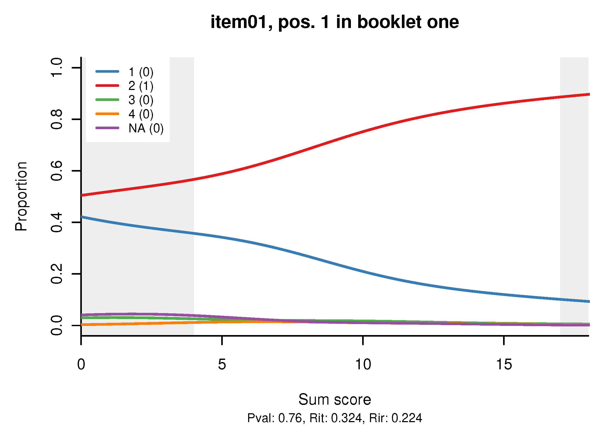
The distractor plot shows a non-parametric regression of the relative frequency of each response alternative, including non-response, on the sum score for the booklet. A separate plot is produced for each booklet that contains the item. The distractor plot for the first item in our small example is shown on Figure 1. The title of the plot shows the item ID, in what booklet the item is featured, and in what position. At the bottom, we see the basic CTT statistics: proportion correct (Pval), item-total correlation (Rit), and item-rest correlation (Rir); the strange acronyms come from practice, including the irritating habit of calling the proportion of correct responses ‘p-value’. The legend shows the responses and the scores that they are assigned—in our example, 2 is the correct response earning an item score of 1, while all other responses are scored 0.

In a well-constructed multiple choice item, the line for the correct response is expected to be monotone increasing (more or less, since it is produced by density estimation of real data). The lines for the wrong responses (the ‘distractors’) should be decreasing, preferably monotone decreasing. The distractor plot makes it easy to spot items with wrong keys, an error that can be corrected easily and without data loss with the touch_rules function. Furthermore, we expect all distractors to ‘work’, i.e., have some plausibility for examinees who do not know the correct response. The item on Figure 1 is badly written, because responses 3 and 4 are too obviously wrong for all examinees, effectively turning the item into a toss-a-coin affair for those of low ability.

The light gray areas, which we call curtains, cover the bottom and the top 5% of the observed data, helping the eye concentrate on the central 90% (there is a parameter to change the 5% to a user-specified value).

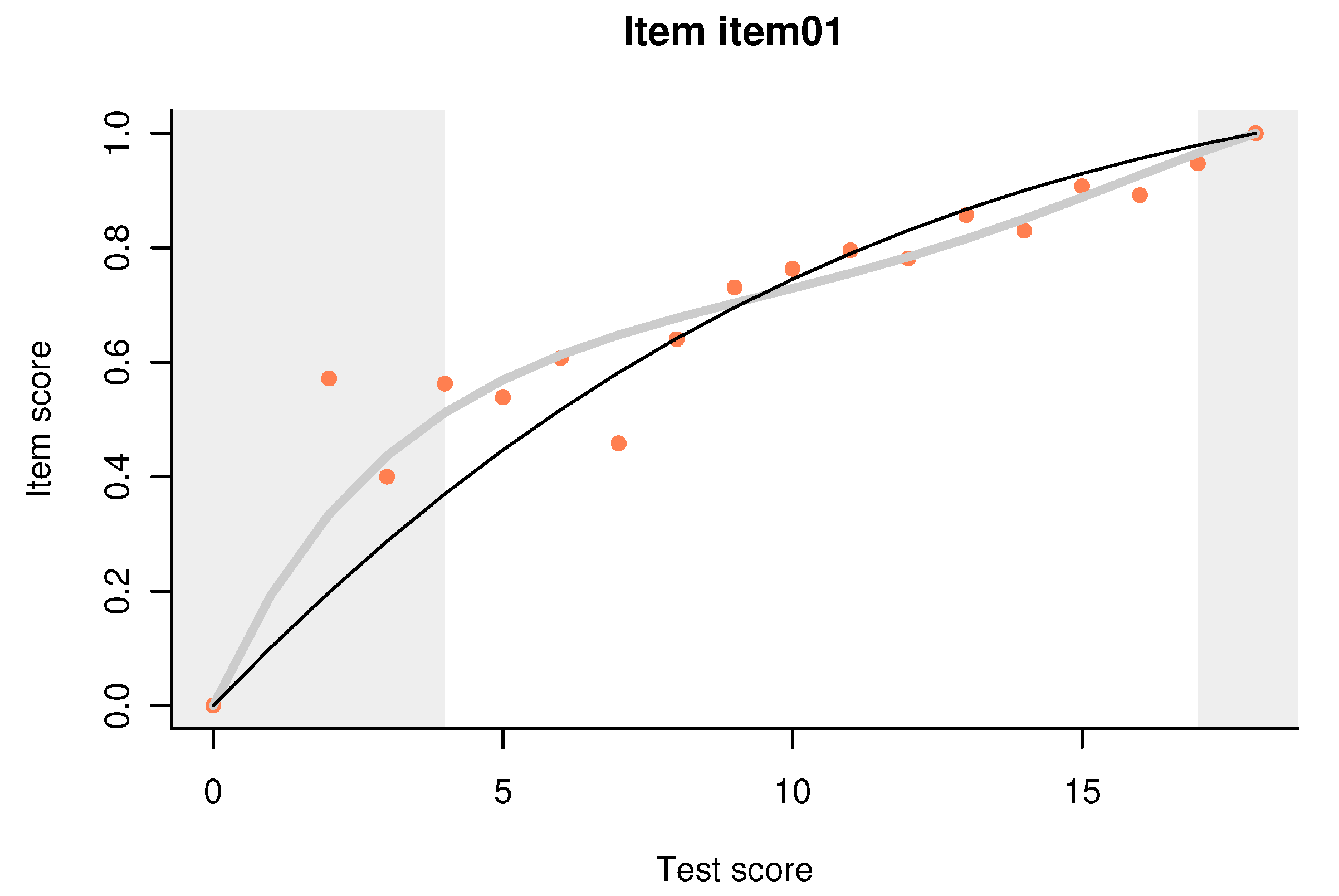
Unlike the distractor plot, the item-total regression plot is model-based. An example using the same Item 1 is shown on Figure 2. To produce such plots, we apply the fit_inter to the data for a specific booklet, and then we pass its output to the generic plot function. The plot compares three item-total regressions. The observed one, shown with light pink dots, is merely the proportion of correct responses to the item among persons with a given total score on the booklet. The thin black line represents the regression predicted by the enorm–the model that will be used to estimate the item parameters for the test as a whole, but here applied locally to just the data for the specific booklet. The thick gray line depicts a similar regression predicted by Haberman’s interaction model [19]. The two models are discussed in some mathematical detail in Section 3; here we provide a brief and intuitive description.

The calibration model in dexter is the extended nominal response model (enorm). This is a nominal response model [9] with known integer score parameters. From the user’s perspective, enorm is not much different from the Rasch model (RM) for the dichotomous items, and the partial credit model (PCM) otherwise. There are some important improvements under the hood, the most visible of which is that we can have partial credit items whose categories are not necessarily coded with adjacent integers. Tests of language proficiency, for example, are abound in such items, and there are situations in longitudinal or comparative surveys when some response categories are not observed in some waves but observed in others. enorm provides an elegant solution to producing consistent (in the general sense) estimates of the item parameters in such situations.

In the original formulation by Haberman, the interaction model (IM) is essentially a Rasch model with the assumption of conditional independence relaxed. When the Rasch model does not fit the data well, there are two options: preserve conditional independence but give up the sufficiency of the sum score (the 2PL model), or give up conditional independence but preserve sufficiency (the IM). The IM is thus a parametric, exponential family model that reproduces the item difficulties, the correlations of the item scores with the total scores on the test, and the total score distribution. In other words, it captures all aspects of the data that are psychometrically relevant, leaving out mostly random noise. It is intuitively clear that the comparison between the two model-based regressions can help us concentrate on systematic differences; in Section 3, we relate it to a long tradition in assessing the goodness of fit in Rasch models.

Note that both axes in Figure 2 refer to observable quantities. In addition, all regressions are pegged to the lower left and upper right corners because all persons with a test score of zero must have an item score of 0, and similar logic applies to the perfect test score. One consequence of this is that the curve for the IM resembles a cubic polynomial when it is flatter in the middle compared to the enorm curve. In our long practice, we have not seen a plot where the pink dots did not cluster around the IM curve: as the sample size increases, the observed regressions get estimated more precisely and the dots get closer and closer to the IM line.

Our example item is dichotomous. We have generalized the IM to polytomous items. The default behavior in that case is to plot the item score in place of the proportion correct, but there is an option to show regressions for the category probabilities instead.

2.4. IRT Analysis: Estimating the Calibration Model

This is easy: fit_enorm(db), $\boxed{\mathrm{Enter}}$, done. Additional flexibility can be achieved by using a predicate. We have already mentioned one possible use: to exclude items not reached from the calibration, but one can think of many others. By popular demand, there is the possibility to fix the parameters for some items to prespecified values. Last but not least, there is a choice between two estimation models: CML [20] or Bayesian estimation through a Gibbs sampler [21]. The function returns an object that is best passed directly and as a whole to other functions, notably the ones that estimate person parameters. Its structure depends slightly on the choice of estimation technique. When CML estimation is used, there is a single set of parameter estimates; if the user chooses Bayesian estimation instead, there will be a set of samples from the posterior distribution of the item parameters. Applied to the output object, the generic coef function will show the parameter estimates and their standard errors; in the case of Bayesian estimation, the output contains the posterior means, the posterior standard deviations, and the 95% highest posterior density intervals. Other statistics can be produced easily: for example, the posterior medians and the medians of absolute deviation (MAD) can be computed as:

m = dexter::fit_enorm(db, method=“Bayes”)
pmed = coef(m, what=’posterior’) |> apply(2, median)
pmad = coef(m, what=’posterior’) |> apply(2, mad)
		  

The generic function plot will produce familiar-looking plots of item fit with the latent variable on the horizontal axis.

2.5. IRT Analysis: Estimating Student Ability

Arguably, IRT has two main practical advantages, and they both relate to the ultimate purpose of educational tests: personal assessment. One is an optimal, theoretically grounded method used to equate the scores gained on similar but distinct test forms, and it is of crucial importance to high-stakes summative assessment. The other is the ability to obtain random samples from a person’s true distribution of (latent) ability given their responses and the item parameter estimates; known as plausible values, these play a vital role in large scale educational surveys [22]. Although related, the two approaches do not mix very well: plausible values are not appropriate in assessment because of the random variability they contain, while the traditional ability estimates are suboptimal in the study of student (sub)populations.

dexter tries to be useful in both situations. For assessment, there are the ability and the ability_tables functions, and for research one can use the plausible_values and plausible_scores function. However, before looking at them, why not ask the more basic question: what if there are no true individual differences in ability? This is similar to an IRT-based test as the reliability is zero, which can be performed with function individual_differences:

dexter::individual_differences(db)
#   Chi-Square Test for the hypothesis that all respondents
#   have the same ability:
# Chi-squared test for given probabilities with simulated p-value
# (based on 2000 replicates)
#   X-squared = 328433, df = NA, p-value = 0.0004998

Function ability takes as minimum arguments a data source and a set of item parameters, and returns a data frame of four variables: the booklet ID, the person ID, the sum score, and the ability estimate. The default estimation method is MLE; the other choices are EAP (expected a posteriori) [23] or Warm’s weighted maximum likelihood estimator (WLE) [24].

Function ability_tables returns a data frame with the booklet ID, the (unequated) booklet sum score, the corresponding (equated) ability estimate, and the standard error of the latter. If grade reporting is done on equated scores, the correspondence can be established easily from the table.

Before proceeding to plausible values and scores and thus to the world of surveys, let us discuss briefly two other functions related to equating and standard setting. Given a reference test with a specified threshold score to pass, function probability_to_pass estimates the equivalent score in a target test, based on ideas from ROC analysis [25,26]. Use the generic coef method to extract the probability to pass for each booklet and score, and the generic plot function to display plots of the probabilities, sensitivity and specificity, and the ROC. This is another method unique to dexter and of interest beyond psychometrics because it extends the popular ROC analysis to situations where a large part of the data is missing by design.

The data driven direct consensus (3DC) method of standard setting was invented by Gunter Maris for the First European Survey of Language Competencies [27]; see also Ref. [28]. The method can be applied traditionally using paper forms, or (preferably) the standard setting sessions may be computerized, in which case the we advise to use the free digital 3DC application available from the Cito website. dexter has functions to support both paper-based and computerized standard setting.

In research or survey settings, the preferred way to approach ability is through plausible values. In spite of the great popularity resulting from their ubiquitous use in large scale assessment projects, it would be wrong to think that plausible values can be computed in one single (and well documented) way. To understand how surveys such as PISA or TIMSS produce them, it is best to go back to the original description [29]. With the parameters of the IRT model (common across countries), the test responses, and the persons’ background variables all being constant, the only factor that makes the plausible values for a given person different is apparently a random sampling from the (multivariate normal) distribution of the regression coefficients of ability on the background variables. This makes it easier to understand why background variables play such an important role in the methodology of these surveys.

dexter takes a different approach to generating plausible values: it uses a highly efficient Gibbs sampler based on composition and rejection algorithms [30]. It does not place so much emphasis on background variables because theory shows that the algorithm will converge to the true distribution of the latent trait—but more efficiently if we can start with a prior that is a reasonably good guess. The package vignette on plausible values discusses an example in which the true distribution of ability is grotesquely bimodal. The sampler will converge to the true distribution with a shorter test if it starts with an appropriate prior; however, with a test of sufficient length the true distribution will be reproduced even if we use a standard normal prior. Currently, dexter offers three kinds of priors:

• A common normal prior for all persons;
• A mixture of two normal distributions not related to any background variable but expected to accommodate many situations (asymmetry, heavy tails, etc.) more flexibly than a normal prior;
• A hierarchical normal prior with a group for each category of one or more nominal background variables.

Similar to ability and ability_tables, the plausible_values function can take the object returned by fit_enorm as one of the parameters. If item parameters have been estimated by CML, the single set of estimates are held constant. A special feature in dexter that, to the best of our knowledge, is not available in any other package, is the ability to condition each draw from the posterior distribution of ability (i.e., each PV) on a different draw from the posterior distribution of item parameters. We believe that this approach better captures all sources of uncertainty inherent to the measurement.

There is also a plausible_scores function. In a design with planned missingness, it produces plausible scores for all items: the person’s actual scores on the administered items are retained, and scores for the ones not administered are predicted based on plausible values. Ref. [31] showed how plausible scores can be used to relax the IRT model in international surveys by applying the market basket approach.

2.6. Measurement Invariance

dexter has two functions to investigate for measurement invariance: DIF is more exploratory and useful when there are known groups (defined by a categorical person property) but no a priori hypotheses on the item side, while profile_plot is applicable when both a person property (groups) and an item property (domains) are known in advance and of interest. Both functions are rather different from the techniques found in other packages, so we need to describe them in some detail.

Arguably, the original problem of differential item functioning (DIF) has subsided over time as item writers have gotten better and better at producing culturally neutral items. However, there are new challenges. On the substantive side, large-scale assessment projects have wider coverage than ever, aiming to compare the output of widely different educational systems. In such a situation, it may be more rewarding to study measurement invariance than merely try to overcome it. On the methodological size, conceptualizing DIF has proved to be more challenging than expected, such that there is still active work on the topic [32].

One of the issues with many techniques used to detect DIF is that they are not invariant to the choice of identification constraints in the IRT model. Imagine a plot of item difficulties estimated in two groups; say boys and girls. The plot will reveal some structure and that structure will not change if we set the difficulty of one or another item to zero for identification purposes. The problem is that the conclusion about which items have DIF can depend dramatically on that arbitrary and fully admissible choice. To avoid this pitfall, Bechger and Maris [33] proposed to concentrate on the structure of DIF rather than the individual item. The idea is to consider, instead of the inter-group differences in item difficulties, the inter-group differences between the matrices of inter-item differences—thus, to turn the study of differential item functioning into a study of differential item pair functioning. Such an approach not only eliminates the impact of the arbitrary identification constraints but also offers additional insight into the structure of DIF by identifying groups of items that ‘behave’ in a similar way.

We will illustrate with a well-known data set on verbal aggression [34], which is available in many R packages, including dexter. A total of 243 women and 73 men answered on a 3-point scale (‘yes’, ‘perhaps’, or ‘no’) how likely they are to become verbally aggressive in 4 different frustrating situations. Further facets include whether the situation was caused by others or by themselves, the intensity of the verbal reaction (curse, scold, or shout); finally, the variable mode indicates whether the verbal behavior would actually be activated or just desired.

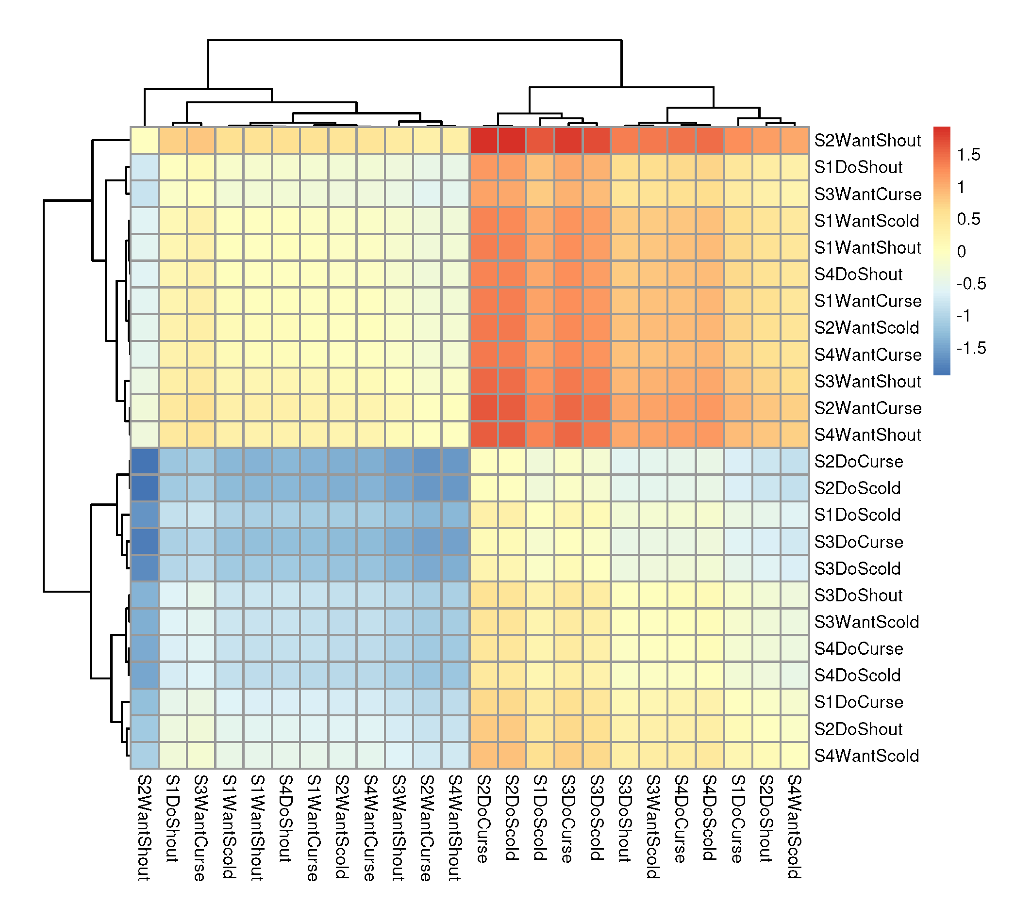
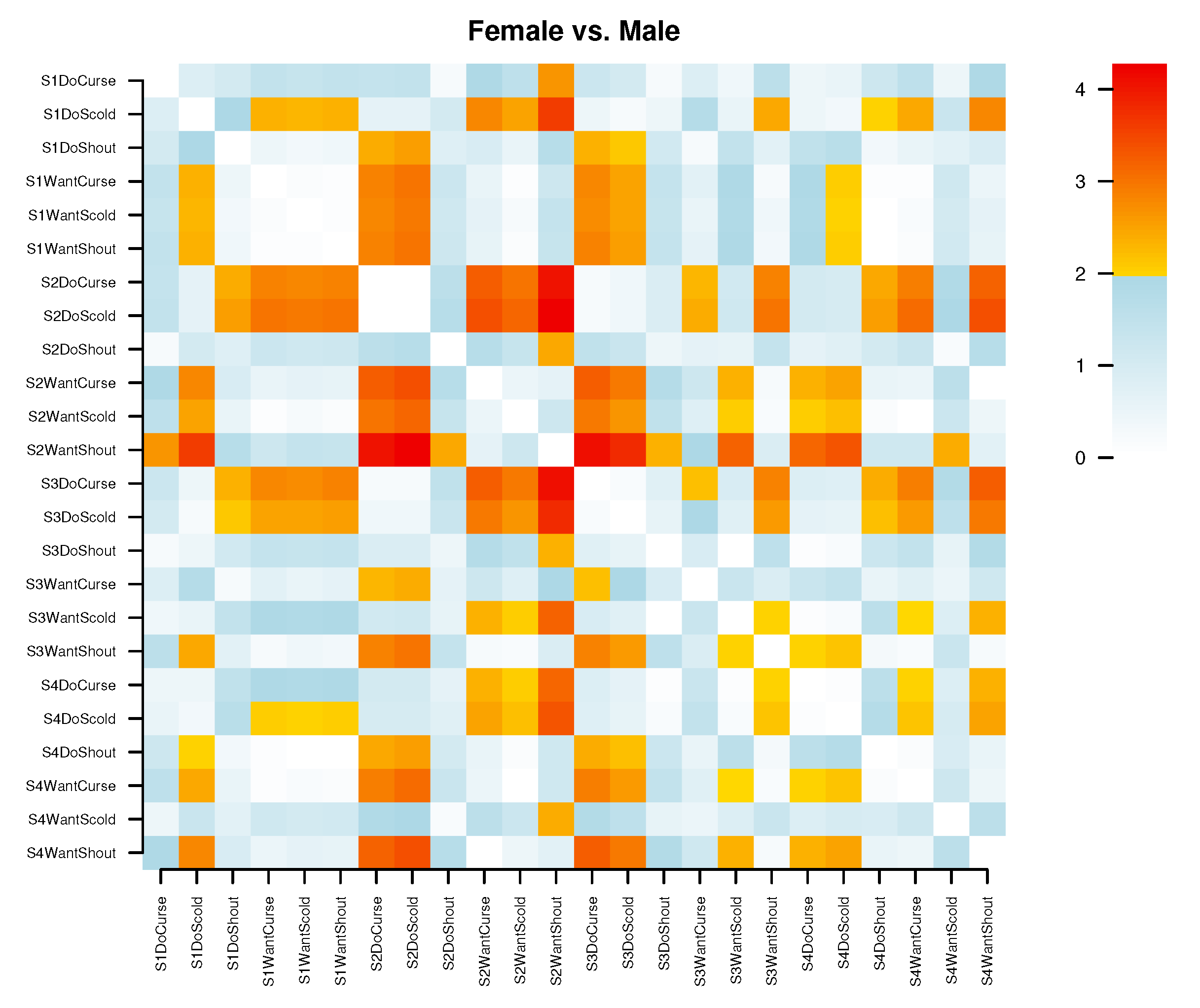
The syntax to compute the DIF statistics is shown below. Note that gender is declared as a person property when the project is created. gender="unknown" defines a default value that will be overwritten by the actual values. The output is an object that contains an overall DIF statistic and two square, skew-symmetric matrices, Delta_R and DIF_pair. Delta_R is computed as the difference between the two square matrices of pairwise differences between the item difficulties, as estimated for men and women separately. DIF_pair is obtained by dividing each element of Delta_R by its estimated variance; thus, it is the matrix of standardized differences, or effect sizes.

dich = dexter::verbAggrRules             # provided with the package
dich$item_score[dich$item_score==2] = 1  # dichotomize the items
db = dexter::start_new_project(dich, ":memory:",
     person_properties=list(gender="unknown"))
dexter::add_booklet(db, verbAggrData, "agg")
d = dexter::DIF(db, ’gender’)
str(d)
#   List of 5
#    $ DIF_overall :List of 3
#    ..$ stat: num 68.8
#    ..$ df  : num 23
#    ..$ p   : num 1.86e-06
#   $ DIF_pair    : num [1:24, 1:24] 0 -0.819 1.005 1.43 1.347 ...
#   $ Delta_R     : num [1:24, 1:24] 0 -0.391 0.484 0.688 0.632 ...
#   $ $ group_labels: chr [1:2] "Female" "Male"
#   $ items       :’data.frame’: 24 obs. of  2 variables:
#    ..$ item_id   : chr [1:24] "S1DoCurse" "S1DoScold" ...
#    ..$ item_score: int [1:24] 1 1 1 1 1 1 1 1 1 1 ...
#   - attr(*, "class")= chr [1:2] "DIF_stats" "list"
		  

The easiest way to understand these matrices is by plotting them as heatmaps. For example, Figure 3 displays a heatmap of the unstandardized differences (Delta_R) produced with the code below. The default clustering of rows and columns readily reveals two groups of items defined primarily by the mode of behavior: ‘Do’ vs. ‘Want’. The relative difficulty of Do and Want items is different for men and women.

rownames(d$Delta_R) = colnames(d$Delta_R) = d$items$item_id
library(pheatmap)
pheatmap::pheatmap(d$Delta_R)
		  

The generic plot function produces a somewhat different display as shown on Figure 4. This is based on the absolute values of the effect sizes (the skew-symmetric matrix becomes symmetric), and the color scheme is calibrated such that values between 0 and 1.96 are shown in shades of blue while those exceeding the critical value progress from yellow to red (the critical value can be changed with parameter alpha). The plot is not clustered but it can be rearranged by passing the item IDs in any desired order: alphabetically, by some item property, sorted by cluster analysis etc.

The generic print function prints the overall DIF statistic, which is highly significant for this example:

print(d)
#   Test for DIF: Chi-square = 68.798, df = 23, p = < 0.0006
		  

These plots are exploratory with respect to the item grouping while the person groups are assumed known. When there are predefined groups of persons and items, a more useful tool is provided by the profiles and profile_plot functions. These follow the logic of profile analysis as proposed by Verhelst [35] although we do not compute all the statistics therein. Profile analysis is an intuitive and robust diagnostic test, and it can be very helpful when the test is not perfectly unidimensional. For example, if we have items on algebra, geometry, and probability, it is our choice (and responsibility) whether to produce three unidimensional tests, a multidimensional test, or at least perform profile analysis as a kind of residuals analysis within the univariate test covering the three domains. Conditional on the overall sum score gained by the person, profile analysis estimates expected domain scores, which can be compared with the observed domain scores. The vector of observed domain scores is called the observed profile, the vector of expected domain scores is called the expected profile, and the vector of their differences is called the deviation profile. If the profiles are purely individual, the deviations can be expected to cancel when aggregating over teachers, schools, or countries; otherwise, they can provide useful information on systematic effects due to differences in teaching quality or policy.

Continuing with the verbal aggression example, we add the item property, mode, to the data base, and we compute the profiles as follows:

dexter::add_item_properties(db, verbAggrProperties)
f = dexter::fit_enorm(db)
p = dexter::profiles(db, f, ’behavior’)
		  

The output is a data frame with the person ID, booklet ID, test score, item property, and observed and expected domain score. Verhelst’s original software, Profile-G, will aggregate individual profiles over groups and provide a covariance matrix. We have not implemented all these features, but profiles can be summarized and analyzed easily in R, for example:

dexter::profiles(db, f, ’mode’) |>
  dplyr::inner_join(get_persons(db)) |>
  dplyr::group_by(gender,mode) |>
  dplyr::summarize(os=mean(domain_score),
    es=mean(expected_domain_score),dv=os-es) |>
  tidyr::pivot_wider(id_cols=’gender’,names_from=’mode’,values_from=’dv’)
#    gender     Do   Want
#    <chr>   <dbl>  <dbl>
#  1 Female -0.191  0.191
#  2 Male    0.635 -0.635
		  

When the item property has two categories (or has been dichotomized in a sensible way), we can use the profile_plot function to build a profile plot similar to the one shown on Figure 5. The two axes show the two domain scores while the gray lines join the points where the two domain scores add up to the same sum scores. For each person group, there is a stairlike line joining the modal (most frequent) combination of domain scores for the person group at each test score. This may sound convoluted, but a single glance at our example plot immediately reveals that, at any overall level of verbal aggressiveness, women “do” less than they “want” as compared to men.

3. Theory and Implementation

3.1. The Extended Normal Response Model (enorm)

As mentioned in the previous sections, dexter concentrates on a purposefully limited range of IRT models. The main model, used to calibrate multi-booklet tests, is the Extended NOminal Response Model (enorm); another model, valuable in evaluating item functioning within a test booklet, is Haberman’s interaction model [19].

Building on the work of Maris, Bechger, and San Martin [21] and Cressie and Holland [36], the enorm is a version of the Nominal Response Model (NRM) [9], where the scoring parameters for the response categories of an item are known integers, and for which the manifest probabilities can be determined in closed form.

The NRM is a generalization of the PCM in which every response category in a polytomous item gets its own score. In the original version of the NRM, the score is a parameter that is estimated (similar to item discrimination in the 2PL). The enorm model implemented in dexter assumes that every response category gets its own integer valued score. Thus, the model differs from the One-Parameter Logistic Model (OPLM, [37]) in the sense that the scores for different categories in a polytomous item need not be equally spaced (i.e., one can have 0, 1, 2, 4 for a 4 category item). This is very convenient in longitudinal or comparative surveys involving items with many categories (typical of language proficiency tests) where some response category may not be observed in a given year or country. The NRM makes it possible to treat the item in a conditional sense, i.e., if we have a PCM with category scores 0, 1, 2, 3, 4, for which category 3 is never observed, we can estimate the model using a conditional PCM (p(response|response not equal to 3)), which is a NRM with a scoring rule 0, 1, 2, 4. In this way parameters with observations in two administrations remain comparable. The Rasch model, the PCM, and the OPLM are all special cases of the enorm.

Let $x_{pij}$ be the dummy-coded response in category j of item i by person p. When possible without causing confusion we will not explicitly distinguish between random variables and their realization. Boldface is used for vectors and matrices, whereas non-boldface variables are scalars. Also, we tend to drop indices in formulae to improve readability, typically the index p when discussing the responses of a generic person. The probabilities for a marginal (with respect to some ability distribution $f\left(t\right)$) NRM are:

$$\begin{array}{cc}\hfill p\left(\mathbf{x}|\mathbf{b},f,\mathbf{a}\right)& ={\int }_0^{\infty }\prod _{i}p\left(x_i\right|b_i,t)f\left(t\right)dt={\int }_0^{\infty }\prod _i\frac{{\prod }_j{\left(b_{ij}{t}^{a_{ij}}\right)}^{x_{ij}}}{1+{\sum }_j{b}_{ij}{t}^{a_{ij}}}f\left(t\right)dt\hfill \\ & =\left(\prod _i\prod _j{b}_{ij}^{x_{ij}}\right){\int }_0^{\infty }{t}^{{\sum }_i{\sum }_j{a}_{ij}{x}_{ij}}\frac{f\left(t\right)}{{\prod }_i\left(1+{\sum }_j{b}_{ij}{t}^{a_{ij}}\right)}dt\hfill \\ \hfill & =\left(\prod _i\prod _j{b}_{ij}^{x_{ij}}\right)\mathcal{E}\left(T^{{\sum }_i{\sum }_j{a}_{ij}{x}_{ij}}|\mathbf{X}=\mathbf{0}\right)p\left(\mathbf{0}\right|\mathbf{b},f,\mathbf{a})\hfill \\ \hfill & =\frac{\left({\prod }_i{\prod }_j{b}_{ij}^{x_{ij}}\right){\lambda }_{{\sum }_i{\sum }_j{a}_{ij}{x}_{ij}}}{{\sum }_s{\gamma }_s\left(\mathbf{b}\right){\lambda }_s}\hfill \\ \hfill & =p\left(\mathbf{x}\right|\mathbf{b},\lambda ,\mathbf{a})\hfill \end{array}$$

(1)

where $\mathcal{E}\left(\right)$ denotes an expected value. For notational convenience we will refer to ${\sum }_i{\sum }_j{a}_{ij}{x}_{ij}$ as $x_{++}$ henceforth (note that this is simply the sum score). Observe that the $a_{ij}$ are not parameters but known integer scores: if item i is answered in category j, then the item score is $a_{ij}$. For every category observed for an item, $b_{ij}$ relates to the number of students scoring in category j of item i, similar to the item difficulty parameter in the simple Rasch model.

Note that whereas the first three lines of the equation are simple mathematical equivalences, the fourth, similar to the formulation of the extended Rasch model in Ref. [21], involves an extension of the model. Specifically, only if

$${\lambda }_s=\mathcal{E}\left(T^s|\mathbf{X}=\mathbf{0}\right)$$

are the third and the fourth lines equivalent. We will refer to the manifest probabilities in the fourth line as the extended NRM (enorm). The advantages of considering the extended model are that the estimation of item category parameters is robust against violation of the postulated population distribution of ability, and the common assumption that students are a simple random sample without multilevel structure.

The functions ${\gamma }_s$ play an important role in what follows, and are defined as:

$${\gamma }_{x_{++}}\left(\mathbf{b}\right)=\sum _{\mathbf{x}\to x_{++}}\prod _i\prod _j{b}_{ij}^{x_{ij}}$$

where $\mathbf{x}\to x_{++}$ means summation over all response vectors $\mathbf{x}$ resulting in a sum score of $x_{++}$. These are a direct extension of the elementary symmetric functions [38] we encounter for the special case of a Rasch model, and we share with these a simple recursive property:

$${\gamma }_s\left(\mathbf{b}\right)={\gamma }_s\left({\mathbf{b}}_{\left(i\right)}\right)+\sum _j{\gamma }_{t-a_{ij}}\left({\mathbf{b}}_{\left(i\right)}\right)b_{ij}$$

where ${\mathbf{b}}_{\left(i\right)}$ denotes the item parameters bar the parameters belonging to item i, and we adopt the convention that ${\gamma }_s=0$ whenever s is not a possible value of $x_{++}$. This recursion is important for two reasons. First, it allows for computing the $\gamma$ functions efficiently, without having to sum over all possible response patterns. Second, it shows that the $\gamma$ function is linear in each of the threshold parameters $b_{ij}$.

To deal with missing data and incomplete designs, consider a design matrix, $\mathbf{D}$, with elements $d_{pij}=1$ whenever person p has responded to item i, and zero otherwise:

$$p\left(\mathbf{x}\right|\mathbf{b},\lambda ,\mathbf{a},\mathbf{D})=\frac{{\prod }_i{\prod }_j{b}_{ij}^{x_{+ij}}{\prod }_k{\prod }_s{\lambda }_{ks}^{n_{ks}}}{{\prod }_k{\left({\sum }_s{\gamma }_s\left({\mathbf{b}}^{\left(k\right)}\right){\lambda }_{ks}\right)}^{n_{k+}}}$$

(2)

where $x_{+ij}={\sum }_p{a}_{ij}{x}_{pij}{d}_{pij}$, $n_{ks}$ denotes the number of students with score s on test form k, and $n_{k+}={\sum }_s{n}_{ks}$ is the total number of students that responded to test form k, with s running over scores on test-form k.

3.2. Estimation

As with the extended Rasch model, we introduce the following reparameterization of the enorm

$${\pi }_{ks}=\frac{{\gamma }_s\left({\mathbf{b}}^{\left(k\right)}\right){\lambda }_{ks}}{{\sum }_t{\gamma }_t\left({\mathbf{b}}^{\left(k\right)}\right){\lambda }_{kt}}$$

in terms of which we obtain the following manifest probabilities:

$$p\left(\mathbf{x}\right|\mathbf{b},\lambda ,\mathbf{a},\mathbf{D})=\frac{{\prod }_i{\prod }_j{b}_{ij}^{x_{+ij}}}{{\prod }_k{\prod }_s{\gamma }_s{\left({\mathbf{b}}^{\left(k\right)}\right)}^{n_{ks}}}\prod _k\prod _s{\pi }_{ks}^{n_{ks}}$$

(3)

from which we see that the score distribution on test form k, ${\mathbf{n}}_k$, follows the multinomial distribution with parameter ${\pi }_k$. Conditional maximum likelihood (CML) entails finding the values of the item-category parameters that maximize the first factor, which is the likelihood conditional on the observed sum scores.

Before moving on, we shortly address the issue of parameter identifiability. From Equation (3) it follows directly that the parameters $\pi$ are identifiable. Regarding the item category threshold parameters, $\mathbf{b}$, they obey the following property:

$$\frac{{\prod }_i{\prod }_j{b}_{ij}^{x_{+ij}}}{{\prod }_k{\prod }_s{\gamma }_s{\left({\mathbf{b}}^{\left(k\right)}\right)}^{n_{ks}}}=\frac{{\prod }_i{\prod }_j{\left(cb\right)}_{ij}^{x_{+ij}}}{{\prod }_k{\prod }_s{c}^s{\gamma }_s{\left(c{\mathbf{b}}^{\left(k\right)}\right)}^{n_{ks}}}$$

which is resolved, for example, by fixing one of the $b_{ij}$ to a particular value.

To estimate the parameters of the enorm  dexter offers the choice between CML or an adaptation of the Gibbs sampler for the extended Rasch model in Ref. [21]. CML has been around for 50 years and is well documented, so here we concentrate on the latter. Adopting a Gamma prior for every parameter, we obtain the following posterior distribution:

$$\begin{array}{c}f\left(\mathbf{b},\lambda |\mathbf{x},\mathbf{a},\mathbf{D}\right)\propto \frac{{\prod }_i{\prod }_j{b}_{ij}^{x_{+ij}}{\prod }_k{\prod }_s{\lambda }_{ks}^{n_{ks}}}{{\prod }_k{\left({\sum }_s{\lambda }_s\left({\mathbf{b}}^{\left(k\right)}\right){\lambda }_{ks}\right)}^{n_{k+}}}\left(\mathrm{likelihood}\right)\hfill \\ \times \prod _i\prod _j{b}_{ij}^{{\eta }_{ij}-1}\exp (-{\rho }_{ij}{b}_{ij})\prod _k\prod _s{\lambda }_{ks}^{{\nu }_{ks}-1}\exp (-{\sigma }_{ks}{\lambda }_{ks})\left(\mathrm{prior}\right)\hfill \end{array}$$

(4)

where ${\eta }_{ij}$, ${\rho }_{ij}$, ${\nu }_{ks}$, and ${\sigma }_{ks}$ are the parameters for the prior for $b_{ij}$ and ${\lambda }_{ks}$, respectively.

A problem with applying the approach for complete data in Ref. [21] with this posterior distribution is that the denominator of the manifest probabilities is, in contrast to complete data, a product, such that we do not immediately obtain full conditional distributions that are tractable. Koops, Bechger, and Maris [39] consider an alternative, data augmentation approach (DA, Tanner and Wong, 1987, Tanner, 1991). The key insight is in the following well known (gamma) integral equation:

$$\frac{\Gamma \left(n\right)}{{\lambda }^n}={\int }_0^{\infty }{y}^{n-1}\exp (-\lambda y)dy$$

(5)

Using this integral equation for every factor in the denominator of our posterior distribution gives the following:

$$\begin{array}{c}f(\mathbf{b},\lambda |\mathbf{x},\mathbf{a},\mathbf{D})\propto \hfill \\ {\int }_{{\mathcal{R}}_{+}^K}\exp \left({\sigma }_{ks}{\lambda }_{ks}\right)\prod _i\prod _j{b}_{ij}^{x_{+}ij+{\eta }_{ij}-1}\exp (-{\rho }_{ij}{b}_{ij})\prod _k\prod _s{\lambda }_{ks}^{n_{ks}{\nu }_{ks}-1}\exp (-{\sigma }_{ks}{\lambda }_{ks})\\ \hfill \times \prod _k{y}_k^{n_k}\exp \left(-\left(\sum _s{\gamma }_s\left({\mathbf{b}}^{\left(k\right)}\right){\lambda }_{ks}\right)y_k\right)d\mathbf{y}\end{array}$$

(6)

where K denotes the number of test forms. The expression inside of the integral is (proportional to) a distribution as well (i.e., $f(\mathbf{b},\lambda ,\mathbf{y}|\mathbf{x},\mathbf{a},\mathbf{D}\left)\right)$. This distribution is extremely simple to simulate by using a Gibbs sampler [40]. Remembering that the $\gamma$ functions are linear in each of their arguments, we see that, for every random variable (e.g., $y_k,b_{ij},{\lambda }_{ks}$), the full conditional distribution is a gamma distribution:

$$\begin{array}{cc}\hfill \left(Y_k\right|\dots )& \sim \mathrm{Gamma}(n_k,\sum _s{\gamma }_s({\mathbf{b}}^{\left(k\right)}){\lambda }_{ks})\hfill \end{array}$$

(7)

$$\begin{array}{cc}\hfill \left({\Lambda }_{ks}\right|\dots )& \sim \mathrm{Gamma}(n_{ks}+{\nu }_{ks},{\gamma }_s({\mathbf{b}}^{\left(k\right)})y_k+{\sigma }_{ks})\hfill \end{array}$$

(8)

$$\begin{array}{cc}\hfill \left(B_{ij}\right|\dots )& \sim \mathrm{Gamma}(x_{+ij}+{\eta }_{ij},\sum _k\sum _s{\gamma }_{s-a_{ij}}\left({\mathbf{b}}_{\left(i\right)}^{\left(k\right)}\right){\lambda }_{ks}{y}_k+{\rho }_{ij})\hfill \end{array}$$

(9)

where we use the shorthand notation … to refer to all other random variables in the joint distribution. Note that this Gibbs sampler shares with CML the property that its computational cost is independent of the number of respondents.

3.3. Goodness of Fit and the Interaction Model

There is a long tradition, going back at least to work by Erling B. Andersen, to evaluate model fit by comparing observed and expected item total regression functions [41]. Andersen’s approach is based on the observation that for the Rasch model, and in fact for any exponential family measurement model, the item parameters can be estimated consistently from responses of students with the same total score. If, with respect to the same identifying constraint, the item parameters for a given item are all the same across all total scores, then the model fits for this item. This original approach is mainly of theoretical interest, as it requires large sample sizes and has many degrees of freedom (and hence low power).

In dexter  we follow Andersen’s general logic with two major differences: we prefer visual checks to formal statistical tests, and we have found a more parsimonious model against which to compare the observed item-total regressions and those predicted by the calibration model: Haberman’s interaction model [19], which we have extended to items having more than two categories. A basic assumption underlying most IRT models is that the responses given by a person are conditionally independent given the latent ability level, $\theta$. For example, in the Rasch model (RM)

$$P(\mathbf{X}=\mathbf{x}|\theta )=\prod _{i}P(X_i=x_i|\theta ,{\beta }_i)\propto \exp (\theta x_{+}+\sum _i{\beta }_i{x}_i).$$

(10)

Haberman [19] relaxes this assumption in the following way:

$$P(\mathbf{X}=\mathbf{x}|\theta )\propto \exp \left[\theta x_{+}+\sum _i{\beta }_i{x}_i+\sum _i\sum _{j>i}({\psi }_i+{\psi }_j)x_i{x}_j\right]$$

(11)

where the additive parameter, ${\psi }_i+{\psi }_j$ captures the strength of the interaction between $X_i$ and $X_j$; the Rasch model obtains a special case when all interaction parameters are zero. Thus, by giving-up on local independence, the Rasch model can be extended without sacrificing the sufficiency of the sum score.

With some algebra, the interaction model (IM) can be rewritten as

$$P(\mathbf{X}=\mathbf{x}|\theta )\propto \exp \left[\theta x_{+}+\sum _i{\beta }_i{x}_i+(x_{+}-1)\sum _i{\psi }_i{x}_i\right]=\exp (\theta x_{+}+\sum _i{\beta }_{x_{+}i}{x}_i)$$

(12)

where ${\beta }_{ri}={\beta }_i+(r-1){\psi }_i$. Written in this way, the IM is similar to the RM except that the item parameters depend linearly on the test sum score. Thus, the IM is not as general as the completely relaxed model used by Andersen, where ${\beta }_{x_{+}i}$ is a parameter for each score and each item; on the other hand, it is not as restrictive as the RM where ${\beta }_{x_{+}i}={\beta }_i$, which is equal for every score, and can even be shown to be more general than the 2PL model. Over the years, we have found that a linear relation between item difficulty and sum score is surprisingly common in large educational data sets, which is another way to say that the IM fits the data. Plots for a couple of real life items are shown on Figure 6.

Rewriting the IM once more, this time as an extended marginal model over the observed frequency distribution of the sum scores, further reveals the useful properties of the model:

$$\begin{array}{cc}\hfill \prod _{p}P\left({\mathbf{x}}_p\right)& =\prod _p\frac{{\lambda }_{x_{p+}}{\prod }_i{\mathbf{b}}_{x_{p+}i}^{x_{pi}}}{{\sum }_s{\gamma }_s\left({\mathbf{b}}_s\right){\lambda }_s}\hfill \\ \hfill & \propto \exp \left(\sum _i{\beta }_i^{*}{x}_{+i}+\sum _i{\psi }_i\sum _p{x}_{p+}{x}_{pi}+\sum _s{n}_s\ln {\lambda }_s\right)\hfill \end{array}$$

(13)

where ${\beta }_i^{*}={\beta }_i-{\psi }_i$. The extended IM is thus seen to be an exponential family model that reproduces the CTT item facilities (proportions correct, irritatingly called p-values by the profession), the item-sum correlations, and the observed score distribution. Since these are the main quantities of interest in classical test and item analysis, it seems fair to say that the extended IM is the model that fits classical test theory.

Furthermore, because the RM and the IM are both exponential family models, it is easy to obtain useful diagnostic displays such as the item-total regressions shown on Figure 2. The observed regressions (proportion of correct responses to the item at each distinct test score) are compared to the regressions predicted by the RM and the IM. In the dichotomous case, these are:

$$\begin{array}{ccc}p(X_i=1|x_{+})& =\frac{{\gamma }_{x_{+}-1}\left({\mathbf{b}}^{\left(i\right)}\right)b_i}{{\gamma }_{x_{+}}\left(\mathbf{b}\right)}\hfill & \left(\mathrm{RM}\right)\\ & =\frac{{\gamma }_{x_{+}-1}\left({\mathbf{b}}^{\left(i\right)}{\mathbf{c}}^{x_{+}}\right)b_i{c}_i^{x_{+}}}{{\gamma }_{x_{+}}\left(\mathbf{b}{\mathbf{c}}^{x_{+}}\right)}\hfill & \left(\mathrm{IM}\right)\end{array}$$

(14)

where $b_i=\exp (-{\beta }_i)$, $c_i=\exp \left({\psi }_i\right)$, and ${\mathbf{b}}^{\left(i\right)}$ denote the item parameters without $b_i$. For polytomous items, dexter offers the choice between regression plots for the item score or regression plots for the probability of each response category. Note that all three regressions involve observable quantities on both axes and avoid circular arguments in assessing the goodness of fit. Comparing the RM to a more relaxed model is consistent with the logic in Ref. [41]; however, while a chi-squared test would give more weight to the least frequent scores, we use the “curtains” on the graph as a reminder that these are areas involving few persons and less precise estimation.

3.4. Ability Estimation

dexter provides the usual estimates of student ability, which are well-known and need not be discussed in detail here (see the previous section for some detail). Staying within the realm of exponential family models makes it easy to provide all the conversion tables needed to equate test forms in practice.

Plausible values (PV [42]) deserve more attention, both for their great theoretical and practical value and because there is considerable variation in the literature and in practical implementations [29]. Marsman et al. [22] enumerate four possible approaches to estimate the distribution of a latent variable, $f(\Theta )$. The PV approach is to use a convenient prior distribution to generate random samples from the posterior distribution given the data and the (estimated) item parameters. Ref. [22] prove that the marginal distribution of these variables, called PV, is a consistent estimator of $f(\Theta )$; they discuss numerous theoretical and practical implications, including the factors influencing the speed of convergence, or what happens if the prior distribution is poorly chosen or an important background variable is not taken into account.

dexter offers a choice between three prior distributions: a standard normal distribution, common for all examinees; separate standard normal distributions for each category of a discrete background variable; or a mixture of two standard normal distributions. The latter option is intended not only for obviously bimodal distribution but should also be able to handle asymmetry, heavy tails, etc. Because we are dealing with models with sufficient statistics for the person and item parameters, it is easy to implement a simple rejection sampler, which boils down to the following idea:

• repeat
•     draw an ability ${\theta }^{*}$ from the prior distribution
•     simulate a response pattern $\mathbf{y}$ for someone with ability ${\theta }^{*}$
• until $y_{+}=x_{+}$
• return ${\theta }^{*}$

As it stands, the algorithm proved to be efficient enough to support the First European Survey of Language Competencies [27]. Further gains in efficiency are possible by stashing the rejected draws for use with candidates with the appropriate total score [43]. In the course of the computations, the priors get updated. In the simplest case of a common normal prior, updating the means (mu) and the standard deviation (sigma) could be done in the following way:

      pvv = var(pv)
      sigma = sqrt(1/rgamma(1, shape=(m-1)/2, rate=((m-1)/2)*pvv))
      pvm = mean(pv)
      mu = rnorm(1, pvm, sigma/sqrt(length(m))
		  

where pv is the latest set of m PV generated. In practice, we update the priors following the multilevel approach in Ref. [44], Chapter 18 (see also the code p. 399f). Updating the mixture prior follows the logic as explained, e.g., in chapter 6 of [45].

3.5. Other Features and Innovations

The purpose of this section is to explain the theoretical and algorithmic fundamentals of dexter. There are many more features, often of an innovative nature, that we cannot cover in detail:

• Our specific approach to DIF, which focuses on item pairs rather than individual items, was introduced in Ref. [33]. We have illustrated it in some detail in the preceding section, so we direct the reader to the original paper for a more formal discussion;
• The use of plausible scores to relax the reliance on common IRT models in comparative research is discussed in Ref. [31] and demonstrated in the next section;
• There is a formal test of individual differences against the null hypothesis that all persons have the same latent ability; it is explained in a package vignette (see the previous section for an example);
• For tests with a defined pass-fail score, there is a novel equating method based on ROC analysis [25]; again, there is a detailed vignette;
• Function latent_cor estimates correlations between latent traits within a dexter project; use an item property to specify the items belonging to each scale;
• A particularly promising application of the models in dexter concerns multi-stage tests with predefined routing rules on observed scores. The theoretical foundations are discussed by Zwitser and Maris [46], and the implementation is in the companion package, dexterMST [47], which also contains a detailed vignette. The major advantage of this approach to adaptivity is that it circumvents many inherent properties of computerized adaptive testing (CAT) that are less attractive in high stakes situations—in particular, unwanted item exposure in both pre-calibration and administration. In contrast, the multi-stage tests implemented in dexterMST are calibrated similar to linear tests, requiring minimal pre-testing.

4. A More Extensive Example

As a larger example of dexter in action, we analyze the cognitive data from the test of mathematics, PISA 2012. We download and parse the data, create a dexter data base, estimate the IRT model, compute five plausible values per examinee, and apply the market basket approach described in Ref. [31].

Note that this is not a tour of dexter or a demonstration of the complete workflow: for example, we omit the test and item diagnostics, which have been discussed already, and which would be the starting point in practice. The purpose is to show dexter in action on a larger project, and to follow up the possible consequences of adopting a different approach to the generation of plausible values or allowing the IRT model to differ across countries.

Analyzing more recent waves of PISA or TIMSS is possible but more tedious because of an unfortunate decision to make the data available in the form of huge binary files for SPSS or SAS; these contain the original and the scored responses, response times, other variables and, of course, an enormous amount of missing data indicators. 2012 is the last year when data was available as ASCII files and syntax files for SPSS and SAS. We use the SAScii package [48] to parse and interpret the SAS syntax; this makes reading the data into R quite easy.

library(dexter)
library(dplyr)
library(tidyr)
library(readr)
library(SAScii)
oecd = "http://www.oecd.org/pisa/pisaproducts/"
url1 = paste0(oecd, "INT_COG12_S_DEC03.zip")
url2 = paste0(oecd, "PISA2012_SAS_scored_cognitive_item.sas")
zipfile = tempfile(fileext=’.zip’)
utils::download.file(url1, zipfile)
fname = utils::unzip(zipfile, list=TRUE)$Name[1]
utils::unzip(zipfile, files = fname, overwrite=TRUE)
unlink(zipfile)  # erase from~disk
dict_scored = SAScii::parse.SAScii(sas_ri = url2)
		

All mathematics items have variable names starting with PM, so it is easy to select them. We change the codes for missing values (7 for N/A and 8 for ‘not reached’) to NA, because distinguishing between them is beyond the scope of this example. The same applies to the careful diagnostic analysis of the responses with CTT and other tools, which is always necessary in practice, and for which dexter is well equipped.

data_scored = readr::read_fwf(
  file = fname,
  col_positions = fwf_widths(dict_scored$width,
     col_names = dict_scored$varname)) |>
  dplyr::select(CNT, SCHOOLID, STIDSTD, BOOKID, starts_with(’PM’))
unlink(fname) # erase from~disk
data_scored$BOOKID = sprintf(’B%02d’, data_scored$BOOKID)
data_scored[data_scored==7] = NA
data_scored[data_scored==8] = NA

Now, start a new dexter project and add the data. First we need to declare all items and their admissible scores in a rules object, which is passed to the start_new_project function.

rules = tidyr::gather(data_scored, key=’item_id’, value=’response’,
      starts_with(’PM’)) |>
  dplyr::distinct(item_id, response) |>
  dplyr::mutate(item_score = ifelse(is.na(response), 0, response))
db = dexter::start_new_project(rules, "pisa2012.db",
  person_properties=list(
    cnt = ’<unknown country>’,
    schoolid = ’<unknown country>’,
    stidstd = ’<unknown student>’
  )
)
		

Add the data for the 21 booklets in a loop. Conveniently, this will deduce the test design automatically:

for(bkdata in split(data_scored, data_scored$BOOKID))
{
  # remove columns that only have NA values
  bkrsp = bkdata[,apply(bkdata,2,function(x) !all(is.na(x)))]
  dexter::add_booklet(db, bkrsp, booklet_id = bkdata$BOOKID[1])
}
rm(data_scored)
		

For later use, we compute a binary item property that indicates whether an item has been asked in all participating countries, and we add it to the data base:

item_by_cnt = dexter::get_responses(db, columns=c(’item_id’, ’cnt’)) |>
   dplyr::distinct()
market_basket = Reduce(intersect, split(item_by_cnt$item_id,
  item_by_cnt$cnt))
dexter::add_item_properties(db,
   dplyr::tibble(item_id = market_basket, in_basket = 1),
      default_values = list(in_basket = 0L))
		

When programmed properly, CML estimation tends to be fast—about 10 s on a rather unpretentious laptop, with most of the time used to fetch the data:

system.time({item_parms = dexter::fit_enorm(db)})
#    user  system elapsed
#   10.80    0.63   11.07
		

Generating the plausible values is also fast: less than 12 s for almost half a million cases:

system.time({pv = dexter::plausible_values(db, parms=item_parms, nPV=5)})
dim(pv)
#    user  system elapsed
#   11.44    0.50   11.93
# [1] 485490      8
		

Comparing against PISA is more work. We need to download a very large data file that contains all the background variables from the student questionnaire, the plausible values, and the sampling and replicate weights necessary to compute the estimates and their standard errors. This necessitated to adjust the timeout option, without which the download may time out. From the large file, we retain only the country identifier and the plausible values.

url3 = paste0(oecd, ’INT_STU12_DEC03.zip’)
url4 = paste0(oecd, ’PISA2012_SAS_student.sas’)
zipfile = tempfile(fileext=’.zip’)
options(timeout = max(300, getOption("timeout")))
utils::download.file(url3, zipfile)
fname = utils::unzip(zipfile, list=TRUE)$Name[1]
utils::unzip(zipfile, files = fname, overwrite=TRUE)
 dict_quest = SAScii::parse.SAScii(sas_ri = url4)
dict_quest = SAScii::parse.SAScii(sas_ri = url4) |>
   dplyr::mutate(end = cumsum(width), beg = end - width + 1) |>
   dplyr::filter(grepl(’CNT|PV.MATH’, varname))
data_quest = readr::read_fwf(file = fname,
   fwf_positions(dict_quest$beg, dict_quest$end, dict_quest$varname))
unlink(zipfile)
unlink(fname)
		

Figure 7 compares the country means of one set of plausible values as estimated by PISA and by dexter. Given that PISA estimates item parameters by MML while dexter uses CML, and that plausible values are computed by different methods (both of which involve random numbers), the correspondence is more than decent.

The country means compared on the plot are calculated from plausible values obtained from a common IRT model for all participating countries. Numerous studies such as Refs. [49,50] have found evidence of DIF in large scale international assessments, and some of them have been quite critical of the current practice, which typically involves fitting country-specific IRT model, removing items with DIF exceeding some prespecified criteria, and then fitting a common model for further analysis and comparison. Zwitser et al. [31] argue that DIF is a natural result from the national efforts to improve education, and its study may be a more rewarding exploit than obtaining a completely DIF-free comparison. They propose an approach using country-specific IRT models that is easy to realize in dexter with the plausible_scores function. The following code selects responses to items that have been asked in all participating countries, fits a different IRT model in each country, and computes plausible scores (there are also some trivial adjustments for items that did not have any correct responses in a few countries). As explained in Section 1, plausible scores are sum scores over all items, where item scores for the items actually asked to the person under the incomplete design are retained ‘as is’, while item scores for the remaining items are simulated from plausible values.

basket = dexter::get_items(db) |>
  dplyr::filter(in_basket == 1) |>
  dplyr::pull(item_id)
 basket = setdiff(basket, c(’PM828Q01’,’PM909Q01’, ’PM985Q03’))
resp = dexter::get_responses(db,
  predicate = item_id %in% basket,
  columns=c(’person_id’, ’item_id’, ’item_score’, ’cnt’))
ps = resp |>
  dplyr::filter (item_id %in% basket) |>
  dplyr::group_by(cnt) |>
  dplyr::do({dexter::plausible_scores(., dexter::fit_enorm(.), nPS=1)})
		

Figure 8 shows country means of a set of plausible scores produced with dexter from country-specific IRT models against the country means of PISA’s first plausible value. The correspondence is quite decent, so it seems that using 68 country-specific IRT models instead of a common model does not make a huge difference. Of course, the items have already been screened for DIF by PISA and their number has been cut in half by the requirement to use only items that have been administered in all countries.

5. Conclusions

An anonymous reviewer has pointed out that every paper needs a conclusion, and we could not agree more—but what conclusions can we draw from presenting our own package? Obviously, we like dexter. We think that its data management capabilities make it unique in its class. An array of diagnostic tools, many of which not available elsewhere, allow for quick identification of problematic items or other issues. The estimation techniques are robust and extremely fast. There are clearly defined boundaries to what the package will or will not do, and much of what it does do is innovative and the subject of numerous original publications.

We were never assigned officially the task to develop software. The package grew gradually—now to provide more efficient or non-standard solutions for projects such as the ESLC, now as a playground for our own psychometric research, including several doctoral dissertations. At some point, a loose collection of functions became shaped up into a comprehensive and handy tool that we felt could be offered to a wider community. However, of course, the final conclusion always belongs to the user.

References

- R Development Core Team. R: A Language and Environment for Statistical Computing; R Foundation for Statistical Computing: Vienna, Austria, 2005; ISBN 3-900051-07-0. [Google Scholar]
- Verhelst, N.D.; Glas, C.A.W.; Verstralen, H.H.F.M. OPLM: One Parameter Logistic Model. Computer Program and Manual; Cito: Arnhem, The Netherlands, 1993. [Google Scholar]
- Kiefer, T.; Robitzsch, A.; Wu, M. TAM: Test Analysis Modules, R Package Version 1.99-6. 2016. Available online: https://CRAN.Rproject.org/package=TAM (accessed on 28 March 2023).
- Chalmers, R.P. mirt: A Multidimensional Item Response Theory Package for the R Environment. J. Stat. Softw. 2012, 48, 1–29. [Google Scholar] [CrossRef]
- Kolen, M.J.; Brennan, R.L. Test Equating, Scaling, and Linking, 2nd ed.; Springer: New York, NY, USA, 2004. [Google Scholar]
- von Davier, A. (Ed.) Statistical Models for Test Equating, Scaling, and Linking; Springer: New York, NY, USA, 2011. [Google Scholar]
- Davier, A.A.; Holland, P.W.; Thayer, D.T. The Kernel Method of Test Equating; Springer: New York, NY, USA, 2004. [Google Scholar]
- González, J.; Wiberg, M. Applying Test Equating Methods; Springer International Publishing: Cham, Switzerland, 2017. [Google Scholar]
- Bock, R.D. Estimating item parameters and latent ability when responses are scored in two or more nominal categories. Psychometrika 1972, 37, 29–51. [Google Scholar] [CrossRef]
- Rasch, G. Probabilistic Models for Some Intelligence and Attainment Tests; University of Chicago Press: Chicago, IL, USA, 1960. [Google Scholar]
- Masters, G.N. A Rasch Model for Partial Credit Scoring. Psychometrika 1982, 47, 149–174. [Google Scholar] [CrossRef]
- Holland, P.W. Measurements or contests? Comments on Zwick, Bond, and Allen/Donoghue. In Proceedings of the American Statistical Association: 1994 Proceedings of the Social Statistics Section, Toronto, Canada, 13–18 August 1994; American Statistical Association: Alexandria, VA, USA, 1995. [Google Scholar]
- International Association of Athletics Federations. IAAF Competition Rules 2018–2019, in Force from 1 November 2017; International Association of Athletics Federation: Monaco, 2017. [Google Scholar]
- Birnbaum, A. Some latent trait models and their use in inferring an examinee’s ability. In Statistical Theories of Mental Test Scores; Lord, F., Novick, M., Eds.; Addison-Wesley: Reading, MA, USA, 1968; Chapter 13; pp. 397–479. [Google Scholar]
- Robitzsch, A.; Lüdtke, O. Some thoughts on analytical choices in the scaling model for test scores in international large-scale assessment studies. Meas. Instrum. Soc. Sci. 2022, 4, 1–20. [Google Scholar] [CrossRef]
- Partchev, I.; Maris, G. Irtoys: A Collection of Functions Related to Item Response Theory (IRT), R Package Version 0.2.2. 2022. Available online: https://CRAN.R-project.org/package=irtoys (accessed on 28 March 2023).
- Wickham, H. Tidy Data. J. Stat. Softw. 2014, 59. [Google Scholar] [CrossRef]
- Hugh-Jones, D. huxtable: Easily Create and Style Tables for LaTeX, HTML and Other Formats, R Package Version 5.5.2. 2022. Available online: https://CRAN.R-project.org/package=huxtable (accessed on 28 March 2023).
- Haberman, S.J. The Interaction Model. In Multivariate and Mixture Distribution Rasch Models: Extensions and Applications; von Davier, M., Carstensen, C., Eds.; Springer: New York, NY, USA, 2007; Chapter 13; pp. 201–216. [Google Scholar]
- Andersen, E.B. The Numerical Solution of a Set of Conditional Estimation Equations. J. R. Stat. Soc. Ser. B (Methodological) 1972, 34, 42–54. [Google Scholar] [CrossRef]
- Maris, G.; Bechger, T.; Martin, E.S. A Gibbs Sampler for the (Extended) Marginal Rasch Model. Psychometrika 2015, 80, 859–879. [Google Scholar] [CrossRef]
- Marsman, M.; Maris, G.; Bechger, T.M.; Glas, C.A.W. What can we learn from plausible values? Psychometrika 2016, 81, 274–289. [Google Scholar] [CrossRef]
- Bock, R.D.; Mislevy, R.J. Adaptive EAP Estimation of Ability in a Microcomputer Environment. Appl. Psychol. Meas. 1982, 6, 431–444. [Google Scholar] [CrossRef]
- Warm, T.A. Weighted Likelihood Estimation of Ability in Item Response Theory. Psychometrika 1989, 54, 427–450. [Google Scholar] [CrossRef]
- Fawcett, T. An introduction to ROC analysis. Pattern Recognit. Lett. 2006, 27, 861–874. [Google Scholar] [CrossRef]
- Krzanowski, W.; Hand, D. ROC Curves for Continuous Data; CRC Press: Boca Raton, FL, USA, 2009. [Google Scholar]
- Ashton, K.; Jones, N.; Maris, G.; Schouwstra, S.; Verhelst, N.; Partchev, I.; Koops, J.; Robinson, M.; Chattopadhyay, M.; Hideg, G.; et al. Technical Report for the First European Survey on Language Competences; Publications Office of the European Union: Luxembourg, 2012. [Google Scholar]
- Keuning, J.; Straat, J.H.; Feskens, R.C.W. The Data-Driven Direct Consensus (3DC) Procedure: A New Approach to Standard Setting. In Theoretical and Practical Advances in Computer-Based Educational Measurement; Springer Nature: Cham, Switzerland, 2017; pp. 263–278. [Google Scholar] [CrossRef]
- Von Davier, M.; Sinharay, S.; Oranje, A.; Beaton, A. The Statistical Procedures Used in National Assessment of Educational Progress: Recent Developments and Future Directions. In Handbook of Statistics; Elsevier: Amsterdam, The Netherlands, 2007; Volume 26, Chapter 32; pp. 1039–1055. [Google Scholar]
- Marsman, M.; Maris, G.; Bechger, T.; Glas, C. Turning simulation into estimation: Generalized exchange algorithms for exponential family models. PLoS ONE 2017, 12, e0169787. [Google Scholar] [CrossRef] [PubMed]
- Zwitser, R.J.; Glaser, S.S.F.; Maris, G. Monitoring Countries in a Changing World: A New Look at DIF in International Surveys. Psychometrika 2017, 82, 210–232. [Google Scholar] [CrossRef] [PubMed]
- Cuellar, E.; Partchev, I.; Zwitser, R.; Bechger, T. Making sense out of measurement non-invariance: How to explore differences among educational systems in international large-scale assessments. Educ. Assess. Eval. Account. 2021, 33, 9–25. [Google Scholar] [CrossRef]
- Bechger, T.M.; Maris, G. A statistical test for Differential item pair functioning. Psychometrika 2015, 80, 317–340. [Google Scholar] [CrossRef] [PubMed]
- Vansteelandt, K. Formal Methods for Contextualized Personality Psychology. Ph.D. Thesis, K. U. Leuven, Leuven, Belgium, 2000. [Google Scholar]
- Verhelst, N.D. Profile Analysis: A Closer Look at the PISA 2000 Reading Data. Scand. J. Educ. Res. 2012, 56, 315–332. [Google Scholar] [CrossRef]
- Cressie, N.; Holland, P.W. Characterizing the manifest probabilities of latent trait models. Psychometrika 1983, 48, 129–141. [Google Scholar] [CrossRef]
- Verhelst, N.D.; Glas, C.A. The one parameter logistic model. In Rasch Models; Springer: New York, NY, USA, 1995; pp. 215–237. [Google Scholar]
- Verhelst, N.D.; Glas, C.A.W.; Van der Sluis, A. Estimation problems in the Rasch model: The basic symmetric functions. Comput. Stat. Q. 1984, 1, 245–262. [Google Scholar]
- Koops, J.; Bechger, T.; Maris, G. Bayesian Inference for Multistage and other Incomplete Designs. 2020; submitted. [Google Scholar]
- Maris, G.; Bechger, T.; Marsman, M. Bayesian Inference in Large-Scale Computational Psychometrics. In Computational Psychometrics: New Methodologies for a New Generation of Digital Learning and Assessment: With Examples in R and Python; Springer Nature: Cham, Switzerland, 2021; pp. 109–131. [Google Scholar]
- Andersen, E.B. A goodness of fit test for the Rasch model. Psychometrika 1973, 38, 123–140. [Google Scholar] [CrossRef]
- Mislevy, R.J. Randomization-based inference about latent variables from complex samples. Psychometrika 1991, 56, 177–196. [Google Scholar] [CrossRef]
- Marsman, M.; Bechger, T.B.; Maris, G.K. Composition algorithms for conditional distributions. In Essays on Contemporary Psychometrics; Springer Nature: Cham, Switzerland, 2022; pp. 219–250. [Google Scholar]
- Gelman, A.; Hill, J. Data Analysis Using Regression and Multilevel/Hierarchical Models; Cambridge University Press: Cambridge, UK, 2006. [Google Scholar] [CrossRef]
- Marin, J.M.; Robert, C.P. Bayesian Essentials with R; Springer: New York, NY, USA, 2014; Volume 48. [Google Scholar]
- Zwitser, R.J.; Maris, G. Conditional Statistical Inference with Multistage Testing Designs. Psychometrika 2013, 80, 65–84. [Google Scholar] [CrossRef] [PubMed]
- Bechger, T.; Koops, J.; Partchev, I.; Maris, G. dexterMST: CML and Bayesian Calibration of Multistage Tests, R Package Version 0.9.3; 2022. Available online: https://CRAN.R-project.org/package=dexterMST (accessed on 28 March 2023).
- Damico, A.J. SAScii: Import ASCII Files Directly into R Using Only a SAS Input Script, R Package Version 1.0.1. 2022. Available online: https://CRAN.R-project.org/package=SAScii (accessed on 28 March 2023).
- Kreiner, S.; Christensen, K.B. Analyses of Model Fit and Robustness. A New Look at the PISA Scaling Model Underlying Ranking of Countries According to Reading Literacy. Psychometrika 2013, 79, 210–231. [Google Scholar] [CrossRef] [PubMed]
- Oliveri, M.E.; von Davier, M. Investigation of model fit and score scale comparability in international assessments. Psychol. Test Assess. Model. 2011, 53, 315–333. [Google Scholar]
Figure 1.
Distractor plot for an example item.
Figure 2.
Item-total regression plot for an example item.
Figure 3.
A clustered heatmap of the matrix of the inter-group differences in the pairwise differences in difficulty between items.
Figure 4.
A DIF plot.
Figure 5.
A profile plot.
Figure 6.
If we estimate item difficulties in groups of respondents with the same test scores, we commonly observe a linear relationship between item difficulty and test score. The left panel shows a Rasch item whose difficulty is independent of the sum score. The panel on the right shows an item conforming to the interaction model.
Figure 7.
Country means of the first plausible value as estimated by PISA and by dexter.
Figure 8.
Country means of the first plausible value as estimated by PISA and plausible scores as estimated by dexter from country-specific IRT models.
Disclaimer/Publisher’s Note: The statements, opinions and data contained in all publications are solely those of the individual author(s) and contributor(s) and not of MDPI and/or the editor(s). MDPI and/or the editor(s) disclaim responsibility for any injury to people or property resulting from any ideas, methods, instructions or products referred to in the content. |
© 2023 by the authors. Licensee MDPI, Basel, Switzerland. This article is an open access article distributed under the terms and conditions of the Creative Commons Attribution (CC BY) license (https://creativecommons.org/licenses/by/4.0/).
Share and Cite
MDPI and ACS Style
Partchev, I.; Koops, J.; Bechger, T.; Feskens, R.; Maris, G. dexter: An R Package to Manage and Analyze Test Data. Psych 2023, 5, 350-375. https://doi.org/10.3390/psych5020024
AMA Style
Partchev I, Koops J, Bechger T, Feskens R, Maris G. dexter: An R Package to Manage and Analyze Test Data. Psych. 2023; 5(2):350-375. https://doi.org/10.3390/psych5020024
Chicago/Turabian StylePartchev, Ivailo, Jesse Koops, Timo Bechger, Remco Feskens, and Gunter Maris. 2023. "dexter: An R Package to Manage and Analyze Test Data" Psych 5, no. 2: 350-375. https://doi.org/10.3390/psych5020024