
Exploring Approaches for Estimating Parameters in Cognitive Diagnosis Models with Small Sample Sizes
by
 , , and
Miguel A. Sorrel
1,* ,
,
Scarlett Escudero
2, 
Pablo Nájera
1 ,
,
Rodrigo S. Kreitchmann
3 and
Ramsés Vázquez-Lira
2 
1
Department of Social Psychology and Methodology, Autonomous University of Madrid, 28049 Madrid, Spain
2
Faculty of Psychology, National Autonomous University of Mexico, Mexico City 04510, Mexico
3
School of Science and Technology, IE University, 28006 Madrid, Spain
*
Author to whom correspondence should be addressed.
Psych 2023, 5(2), 336-349; https://doi.org/10.3390/psych5020023
Submission received: 24 March 2023
/
Revised: 20 April 2023
/
Accepted: 25 April 2023
/
Published: 27 April 2023
(This article belongs to the Special Issue Computational Aspects and Software in Psychometrics II)
Abstract
:Cognitive diagnostic models (CDMs) are increasingly being used in various assessment contexts to identify cognitive processes and provide tailored feedback. However, the most commonly used estimation method for CDMs, marginal maximum likelihood estimation with Expectation–Maximization (MMLE-EM), can present difficulties when sample sizes are small. This study compares the results of different estimation methods for CDMs under varying sample sizes using simulated and empirical data. The methods compared include MMLE-EM, Bayes modal, Markov chain Monte Carlo, a non-parametric method, and a parsimonious parametric model such as Restricted DINA. We varied the sample size, and assessed the bias in the estimation of item parameters, the precision in attribute classification, the bias in the reliability estimate, and computational cost. The findings suggest that alternative estimation methods are preferred over MMLE-EM under low sample-size conditions, whereas comparable results are obtained under large sample-size conditions. Practitioners should consider using alternative estimation methods when working with small samples to obtain more accurate estimates of CDM parameters. This study aims to maximize the potential of CDMs by providing guidance on the estimation of the parameters.
1. Introduction
Cognitive diagnostic models (CDMs) are confirmatory latent class models with applications in educational assessment, clinical psychology, and industrial–organizational psychology, among others (e.g., [1,2,3,4]). Specifically, by adopting an item response function that accounts for the relationship between the assessed attributes (skills, cognitive processes, competences) and a Q-matrix with the dimensions J items × K attributes, CDMs yield the classification of examinees into one of the possible latent profiles denoted by . There are latent classes in the most common case of dichotomous attributes, although there are models that consider polytomous attributes [5]. Several introductions to these models are available, discussing the most recent developments and their estimation in R [6,7].
1.1. The DINA Model
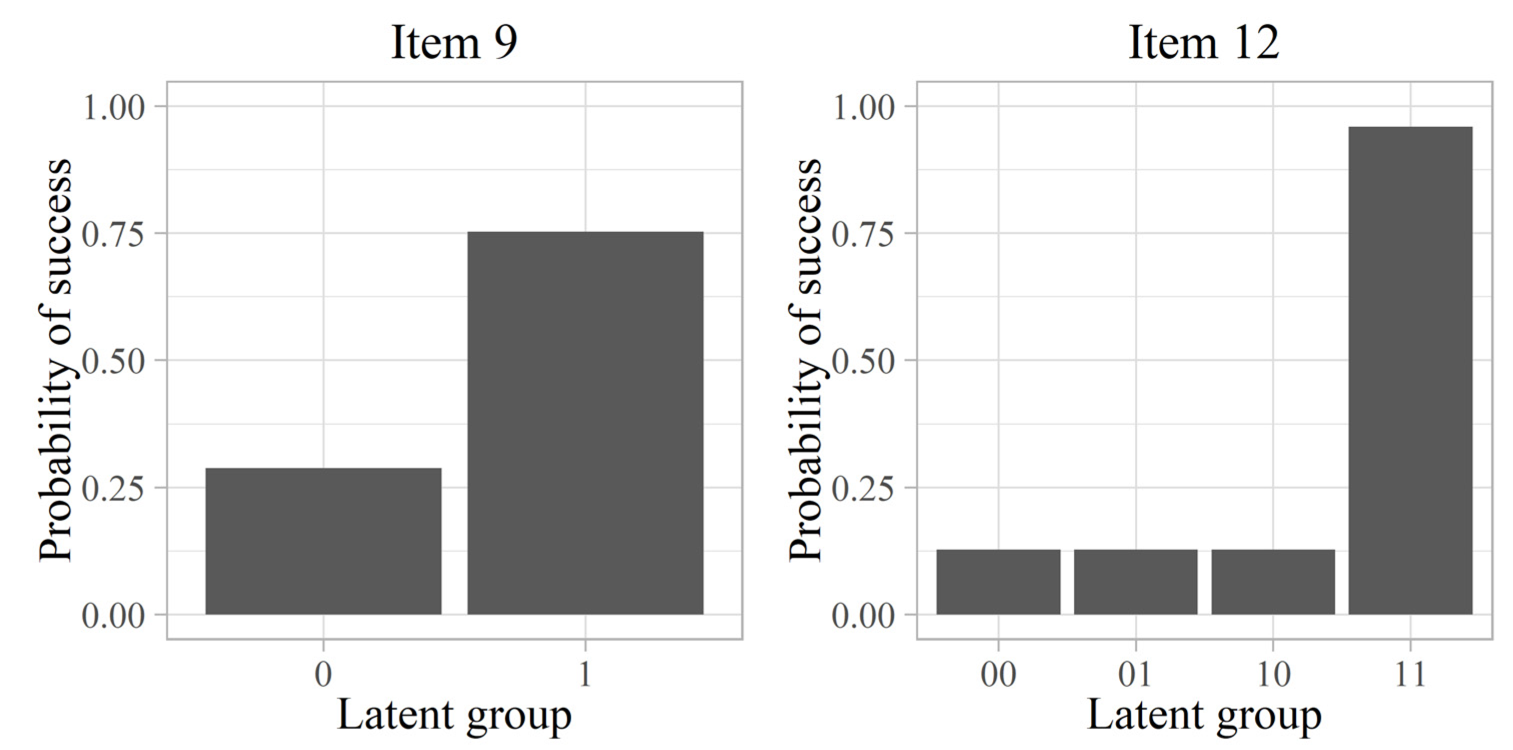
Recently, Sessoms and Henson (2018) [8] conducted a review of the empirical applications using CDM published to date. The authors reported that the most commonly applied model was the deterministic input noisy output “and” gate (DINA) model [9]. One of the reasons for preferring this model is its ease of interpretation, as opposed to more complex models. Specifically, for a given item j, regardless of the number of attributes assessed by that item (), the DINA model separates examinees into two latent groups: those who possess all the attributes required by that item () and those who do not master at least one of those attributes (). For example, for an item whose Q-matrix vector is , i.e., it measures the first two attributes evaluated in a test but not the third, the group would be composed of individuals with and and the group would be composed of all the others (, , , ,, and ). A representation of this model for one item measuring one attribute and another item measuring two attributes is shown in Figure 1. The DINA model considers two parameters per item, the probability of failure for denoted as (slip parameter) and the probability of success for denoted as (guessing parameter). In both cases, although the items vary in complexity (i.e., the number of attributes evaluated), only these two parameters are estimated. It is noticeable in the figure how item 9 has higher guessing and slip parameters. A common measure of item discrimination is , which indicates the difference in success probability between groups and .
It should be noted that the estimated item parameters will be used not only to classify examinees, but also in the evaluation of the model fit or the computation of the reliability indices, among other analyses. How difficult or easy it is to estimate these parameters is related to the complexity of the model and Q-matrix (i.e., the number of parameters to be estimated) and the available sample size. In this study, we focus on the DINA model as opposed to other more general models, such as its generalized version, the generalized DINA model (G-DINA; [11]), because it allows us to isolate the complexity factor of the model, as the DINA model always has two parameters per item regardless of the complexity of the item q-vector. Moreover, previous studies have already explored the topic of model complexity (e.g., [12]). This will allow us to focus on the effect of sample size. According to Sessoms and Henson (2018) [8], the DINA model has been applied under widely varying sample-size conditions, with sample sizes as low as 109 and as high as 71,000. In their review, they found that, in general, the sample size varied greatly from study to study, with the mean being 1787.77. General models such as G-DINA were mostly applied under conditions of larger sample sizes. Nevertheless, and this is why it is particularly interesting to put the focus on the DINA model, it is worth noting that CDMs are born in the field of education with the primary objective of providing diagnostic feedback to students [13]. This redounds to the idea that studying parameter recovery under the DINA model in low sample-size situations is particularly relevant. Some recent applications in this context have been conducted with school and university samples [14,15].
1.2. Estimation Procedures
As in traditional item response theory, parameter estimation can take either a frequentist or a Bayesian approach. The frequentist approach operationalized as the marginal maximum likelihood estimation with Expectation–Maximization (MMLE-EM) algorithm is the most commonly employed estimation procedure in practice. Specifically, among the studies collected in Sessoms and Henson (2018) [8], in 13 of the 36 articles reviewed (36%) the DINA model is estimated. Only one of these studies reports that a different estimation procedure from MMLE-EM was applied, and this alternative was Markov chain Monte Carlo (MCMC) with Gibbs sampling [16]. It is interesting to note that of those 13 studies, this is the one that had the smallest sample size (109), although another of the studies also had a small sample size of 144 [17]. This certainly makes sense considering that the MMLE-EM approach is easily accessible through two popular R packages for CDM, such as the GDINA R package [18,19] and the CDM R package [20,21]. As of March 2023, both packages together have accumulated almost half a million downloads on CRAN. Other packages such as cdmTools [22,23] and cdcatR [24] offer additional analyses taking as input the models calibrated with the first two packages. In summary, it is to be expected that the ease of access to MMLE-EM estimation will keep it as the most popular estimation procedure.
Due to this context, it is important to note that recently there have been articles pointing out that in situations of low sample size, MMLE-EM can have boundary problems, i.e., that the parameter estimate (in this case a probability of success bounded between 0 and 1) converges toward the boundary of the parameter space [25,26]. It is for this reason that different alternatives for estimating item parameters or classifying individuals have been proposed in the literature. In these situations, it might be more convenient to adopt a Bayesian approach that prevents the aforementioned problems [27,28].
An approach that has started to gain popularity in the psychometrics field is a Bayesian use of MCMC methods. The frequentist approach considers model parameters as fixed and provides point-estimates for those parameters. On the contrary, the Bayesian approach seek the posterior distribution of the model parameters. This posterior distribution is typically represented in terms of posterior mean and standard deviation, which would be the equivalent to the frequentist point-estimate and standard errors. MCMC methods are a class of algorithms for sampling from a probability distribution. To perform this process, it is necessary to define a complete likelihood and prior distribution for the parameters, which will be used to calculate a combined posterior distribution. MCMC techniques are employed to produce samples from this joint posterior distribution. Specifically, these methods use the previous sample values to randomly generate the next sample value, generating a Markov chain, estimating a posterior distribution. Each random sample is used to generate the next random sample, hence the chain [29]. One particular MCMC method, the Gibbs sampler, is very widely applicable and efficient to a broad class of Bayesian problems. Gibbs sampling is a special case of the Metropolis–Hastings algorithm, which is a generalized form of the Metropolis algorithm [30]. Gibbs sampling is applicable in situations where the joint distribution is not explicitly known or it is challenging to directly obtain samples from it, but the conditional distribution of each variable is known and can be more easily sampled from. Thus, the basic idea of Gibbs sampling is to iteratively sample from the conditional distribution, rather than drawing directly from the joint posterior distribution [31]. This sampler is used by default in popular software such as Just Another Gibbs Sampler (JAGS) [32]. Another variation of MCMC methods is the Hamiltonian Monte Carlo (HMC), which uses the derivatives of the density function being sampled to generate efficient transitions spanning the posterior. It employs numerical integration to simulate Hamiltonian dynamics approximately, followed by a Metropolis acceptance step to correct the simulation. Compared to Gibbs sampling, HMC is more efficient in obtaining samples with lower autocorrelations. Thus, the effective sample size for HMC is usually much higher than the other MCMC methods. One software that generates random representative samples from a posterior distribution implementing HMC is Stan [33]. Stan operates with compiled C++ and allows greater programming flexibility, which is useful for complex models, providing solutions that JAGS sometimes cannot [31].
Apart from MMLE-EM and MCMC estimation, several alternatives have been proposed in recent years to implement CDM in low sample-size situations. A very recent one is the proposal by Ma and Jiang (2021) [34], who developed a Bayes modal estimation (BM) based on the MMLE-EM estimation but incorporating prior distributions for the items parameters. Another route is to renounce estimating item parameters in low-sample situations, adopting a nonparametric procedure such as that proposed by Chiu and Douglas (2013) [35], which compares observed responses to ideal response patterns. A recent proposal is to reduce the model as much as possible, estimating a single parameter that accounts for the differences between observed and ideal response patterns [36].
While these all turn out to be plausible alternatives, it is important to note that there is no study to date that has captured the gain with respect to MMLE-EM. Although there are some previous studies exploring this topic [34,37], they have compared some alternatives but not all of them. The goal of the current study is to address this topic through a simulation study and an empirical illustration. Therefore, this study redounds to the line of work on the use of CDM in small samples [38] with the aim of concluding the best way to estimate item parameters, so as to serve as a guide for future empirical applications seeking to maximize the potential of CDM. We hypothesized a better performance of the different alternatives against MMLE-EM in situations of low sample size and no differences in situations of large sample size.
2. Materials and Methods
2.1. Item Parameter Estimation Methods and Attribute Profile Classification
We implemented different estimation methods to estimate the DINA model item parameters in R [39]:
- -
- For the MMLE-EM method we used the GDINA package. Sen and Terzi (2020) [40] compared different software (CDM R package, flexMIRT, Latent GOLD, mdltm, Mplus, and OxEdit) to estimate the DINA model using this estimation procedure. The differences between estimated item parameters were always marginal. The same holds true for Rupp and van Rijn’s (2018) [41] comparison of the R packages GDINA and CDM, whereby the results reported here for the GDINA R package should be largely generalizable to any other software. Details on MMLE-EM estimation can be found in de la Torre (2009) [42]. This procedure uses the marginalized likelihood of the data:where is the marginalized likelihood of the response vector for examinee i and is the prior probability of the attribute vector . In the same paper, the author provides the ML estimators of the guessing and slip parameters. Specifically, and , where () indicates the number of people in () and () indicates how many of those people get item j right. As specified by default in the package, three sets of starting values have been generated and the best set according to the observed log-likelihood is used. This is performed to avoid the problem of local optima using MMLE.
- -
- For the BM estimation, we applied the R code provided by Ma and Jiang (2021) [34]. The BM or posterior model estimation incorporates prior information about model parameters into the EM algorithm. In a way, it can be seen as a computationally efficient version of MCMC estimation. Specifically, the BM estimation of the guessing parameter adopts ), where and are the parameters for a beta distribution . The same consideration is taken for the slip parameter. The interested reader is referred to the appendix of the original article for more technical details. For BM and MCMC (described below), initial values were drawn from a uniform distribution between 0.10 and 0.30. A β(5, 25) distribution was used for the item parameters. This is a distribution centered at 0.166 (i.e., examinees are expected to produce guessing and slip 1/6 (=5/(5 + 25)) of the times. We refer to this procedure as BM-info. On the other hand, in all cases the maximum a posteriori estimator was adopted as the estimator of the attribute profile of the examinees using a uniform distribution as the prior distribution.
- -
- For the MCMC estimation, we used the Gibbs sampling estimator using the JAGS code via the R package R2jags [43] provided by Zhan et al. (2019) [44]. The algorithm was set to 2500 iterations and 500 burn-in in two chains as performed by Culpepper (2015) [27]. We considered both a non-informative, flat prior [MCMC-unif; β(1, 1)] and an informative prior [MCMC-info; β(5, 25)]. We tested that this estimator provided almost identical results as the ones that could be obtained using Stan via the R code provided by Lee (2016) [45] and the rstan package [46]. The computation times with Stan were considerably slower than those of JAGS. For example, in the simulation study, for a replication with 100 examinees, JAGS required 1.108 min and Stan 11.252. Since the results were basically identical, we conducted the complete study using JAGS. Another reason to prefer this software is that Zhan et al. (2019) [44] provide in their article the codes for other models besides DINA, so the researcher interested in applying other models can take advantage of this.
These four procedures (MMLE-EM, BM-info, MCMC-unif, and MCMC-info) provide estimates of the guessing and slip parameters and use those estimates to classify examinees. On the other hand, as a baseline for assessing the performance of the different estimation procedures in classifying examines, two other procedures specifically designed to classify examinees under low sample-size conditions were included:
- -
- The nonparametric classification (NPC) method [35] was implemented using the NPCD package [47]. No parameter estimation is conducted in the NPC method; instead, ideal response patterns () are formulated for each possible attribute profile based on a conjunctive, , or disjunctive, ), condensation rule. Here, we adopted the conjunctive condensation rule that accommodates non-compensatory processes such as the DINA model. Then, examinees’ observed response patterns () are compared with the attribute profiles’ ideal response patterns with the so-called Hamming distances, , so that the attribute profile assigned to examinee i is the one that minimizes such distances. Note that ties can be found for two or more attribute profiles; in this case, the assigned attribute profile would be randomly selected among those with the lowest Hamming distance.
- -
- The Restricted DINA model (R-DINA) [36] was estimated with the cdmTools package [23]. In the R-DINA model, a single parameter φ is estimated for the whole model, which is defined as the proportion of observed responses that depart from the ideal responses. Making a comparison with the more traditional DINA model, . The estimation procedure used in the package provides equivalent results to the MMLE-EM estimation. The R-DINA model has been shown to provide the same attribute profile classifications as the NPC method when no prior information on the attribute joint distribution is incorporated. Small differences can be found between both methods due to the randomness implied in the selection of the attribute profile when there are ties between two or more attribute profiles (i.e., same, lowest Hamming distance or, equivalently, same, largest likelihood).
Finally, Kreitchmann et al. (2022) [25] proposed a multiple imputation procedure (MMLE-EM with MI) to account for the item parameter estimates uncertainty in computing the classification accuracy estimates. Since this procedure is available in the cdmTools package, we implemented it in order to have a baseline for comparison of the classification accuracy estimates, which is one of the dependent variables described in the following sections.
2.2. Data
2.2.1. Simulation Study
The simulation study consisted of simulating two cases of samples of 100 and 2000 observations with a uniform distribution for the attribute joint distribution. A total of 100 replicas per condition were implemented to assure the consistency of the results. The Q-matrix used in the data generation and model estimation was the sim30DINA$simQ Q-matrix included in the GDINA R package. In this Q-matrix, there are 30 items measuring 5 attributes. Each attribute is measured by 12 items, and there are 10 one-attribute items, 10 two-attribute items, and 10 three-attribute items. This Q-matrix includes two identity matrices and satisfies the requirements for model identification [48]; it has been used in multiple previous simulation studies [34,42,49]. The item quality was set to a medium level by setting . Thus, the generating model coincides with the R-DINA since DINA reduces to R-DINA when [36], with = 0.20 in this case. It is common to generate item parameters in this way in simulation studies as it will allow the recovery of item parameters to be studied in a simple way [2,42]. Note that the prior distributions for item parameters used for Bayesian methods are not centered at 0.20. This was executed intentionally to facilitate a fair comparison with MMLE-EM. In a real situation, prior distributions should be established by the researcher considering the available evidence (e.g., behavior of similar items, the expected quality of the items). In addition, note that in small sample sizes, the established prior distribution can have important effects on the posterior. As a final note regarding the prior distribution, it is important to clarify that although both BM and MCMC require establishing a prior distribution, the effect of this choice may be greater for BM. This is because BM regularizes the ML estimation using that prior distribution, while MCMC will only take the prior distribution as a starting point but will generate a posterior distribution through sampling. These factors (test length, number of attributes evaluated, and item quality) were kept fixed at an intermediate level, since the goal of the study is simply to illustrate the effect of sample size on parameter estimation for a given condition. The levels chosen are representative of the empirical or usually simulated conditions encountered: the mode in number of attributes assessed is 4 and the median 6.5 [8] and 30 items and are frequently considered as intermediate levels of these factors (e.g., [34,49]).
2.2.2. Empirical Study
The empirical study used the dataset and Q-matrix of the Fraction–Subtraction data [10] available in the GDINA R package. This test consisted of 20 items measuring 8 attributes related to fraction addition and subtraction and was responded to by 536 middle school students. The attributes being measured were (1) convert a whole number to fraction, (2) separate a whole number from fraction, (3) simplify before subtraction, (4) find a common denominator, (5) borrow from the whole number part, (6) column borrow to subtract the second numerator from the first, (7) subtract numerators, and (8) reduce answers to simplest form. This database was chosen because it has been used in multiple previous CDM studies and an acceptable fit to the DINA model has been reported [50,51].
To illustrate the effect of sample size on the estimation of item parameters and the robustness of each estimation procedure, we considered the estimates made with the total sample as a baseline and sampled 20 replicas of 100 random examinees as an example of a small database. On this small database, we ran all the estimation procedures and compared the results (item parameters, attribute profile, and classification accuracy estimates) obtained with those estimated with the total sample considering the values obtained with the complete sample as the “true” values. The item parameters obtained with each of the estimation methods are reported in Table 1. Taking as a reference the estimates for MMLE-EM, it can be observed how in general guessing and slip differ for the same item as is the case of item 13, with a guessing close to zero (0.013) but a high slip (0.335), and guessing and slip also differ across items, with items such as item 2 where guessing and slip are low (0.016 and 0.041, respectively) and others such as item 8 where guessing and slip are high (0.444 and 0.182, respectively). That is, contrary to what occurs in the simulation study, these estimates would match the DINA model, which allows estimating different guessing and slip for each item and a loss of fit would be expected with the R-DINA, which estimates a single parameter common to all items. Consistent with this, the relative fit statistics led to retain the DINA model. (AICDINA = 9394.606 vs. AICR-DINA = 11,686.39 y BICDINA = 10,658.430 vs. BICR-DINA = 12,783.130).
2.3. Dependent Variables
The dependent variables we computed were the mean absolute bias (MAB) of the guessing and slip parameters (Equation (2)), the proportion of correctly classified attribute vectors (PCV; Equation (3)), and the reliability bias (Equation (4)).
where is the indicator function and is the estimated test-level classification accuracy which is computed from the average of the posterior probability of the attribute profiles [19,52].
In the empirical study, we computed the difference or agreement between the item parameters of each sample size, attribute classifications, and reliability estimate. The mean of the 20 replicas is presented as the value of each variable. In both studies, we also stored the time required to complete the estimation for each of the item parameter estimation procedures. The simulation was conducted in a desktop PC 11th Gen Intel(R) Core(TM) i9-11900 @ 2.50GHz 2.50 GH with 32GB of RAM.
3. Results
3.1. Simulation Study
The results of the simulation study are summarized in Table 2. Note that to evaluate the guessing and slip parameters only MMLE-EM, BM-info, MCMC-unif, and MCMC-info are considered because NPC and R-DINA do not estimate guessing and slip parameters. Table 2 also specifies the PCV and reliability bias of the true, generating model where guessing and slip parameters are exactly the generating values (i.e., 0.20). Values in each replica were averaged and those are the results presented in Table 2, together with standard deviations.
First, all procedures converged in results when the sample size is large. The MAB of guessing and slip was very close to zero (around 0.01 and 0.02, respectively, in all cases). The PCV was very close to that of the true, generating model (.692), indicating that 69% of the examinees were correctly classified on their attribute profile and the bias in reliability was also virtually 0. It is only when the sample size is small that differences among the methods appear. The method offering the most accurate estimation of item parameters was MCMC with informative priors, with MAB around 0.03 for both guessing and slip. The results for BM-info were slightly worse, with the MAB for guessing at 0.033 (vs. 0.029 for MCMC-info) and for 0.044 (vs. 0.033 for MCMC-info) for slip. The method leading to the poorest item parameter recovery was MMLE-EM (0.048 and 0.089 for guessing and slip, respectively), similar values to those obtained by MCMC with a uniform prior distribution. Thus, Bayesian procedures (BM-info and MCMC) with informative priors led to better item parameter recovery. It is worth noting how it can be consistently observed that the error in the slip estimation was always larger than for guessing. This makes sense if we consider that the slip parameter refers to a group () that can be expected to be always less numerous under the DINA model (with respect to ), given its non-compensatory nature.
These differences in guessing and slip estimation translated into differences in classification accuracy. Thus, among the procedures for the estimate of the DINA model, MCMC-info was the best method at classifying examinees (PCV = 0.688) and MMLE-EM the worst (PCV = 0.622). The procedures specifically designed to classify examinees in small samples also showed comparable performance to MCMC-info (PCV for NPC and R-DINA was equal to 0.692 and 0.690, respectively).
Finally, it was also observed that the lack of precision in the item parameters translated into a bias in the reliability estimation. Specifically, MMLE-EM obtained a very high bias (0.191), which implies a considerable overestimation of reliability. It is worth noting here that the multiple imputation procedure (MMLE-EM with MI) effectively managed to eliminate that bias (0.000). R-DINA also provided unbiased estimates of reliability. Again, MCMC-info offered slightly better results than those of BM-info (0.041 vs. 0.086), even though both methods overestimated reliability.
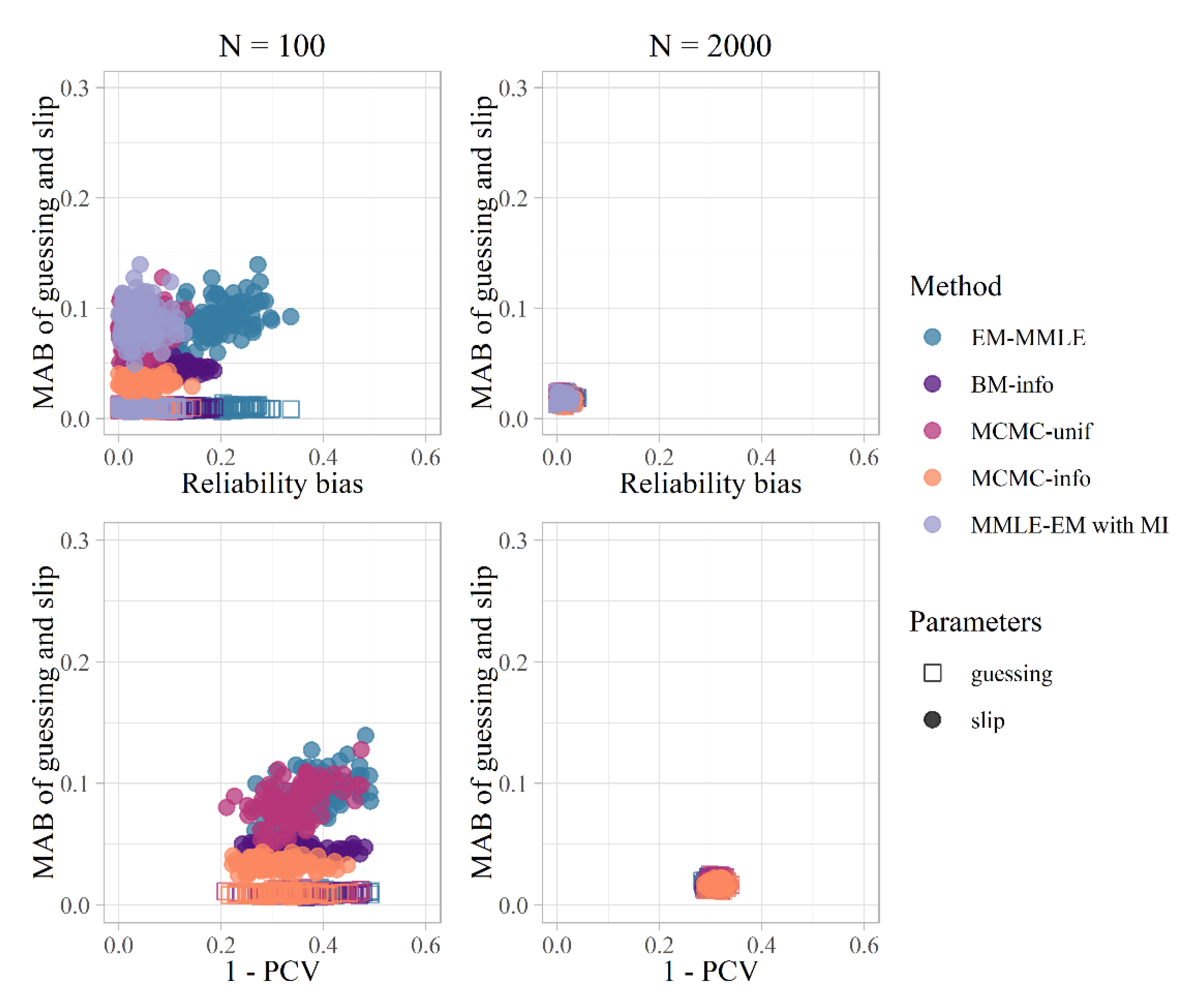
To better understand the relationship between the three dependent variables, Figure 2 illustrates the relationship between MAB of guessing and slip, the proportion of incorrectly classified attribute vectors (1-PCV), and the reliability bias, showing the result obtained for each of the generated databases. It is apparent how, under n = 2000, there is no difference in performance between the methods, i.e., the points overlap, but that under n = 100 there is an direct relationship between MAB of guessing and slip and 1-PCV and reliability bias. It can be observed at a descriptive level that for MCMC-info the replicate-to-replicate variability was somewhat lower.
Regarding computing times, the fastest calculations were by MMLE-EM, BM-info, NPC, and R-DINA; despite the sample size, each was completed in less than a second. Meanwhile, the MCMC estimations were considerably longer, taking on average about one minute for each estimation in the small sample-size condition and 30 min in the large sample-size condition.
3.2. Empirical Study
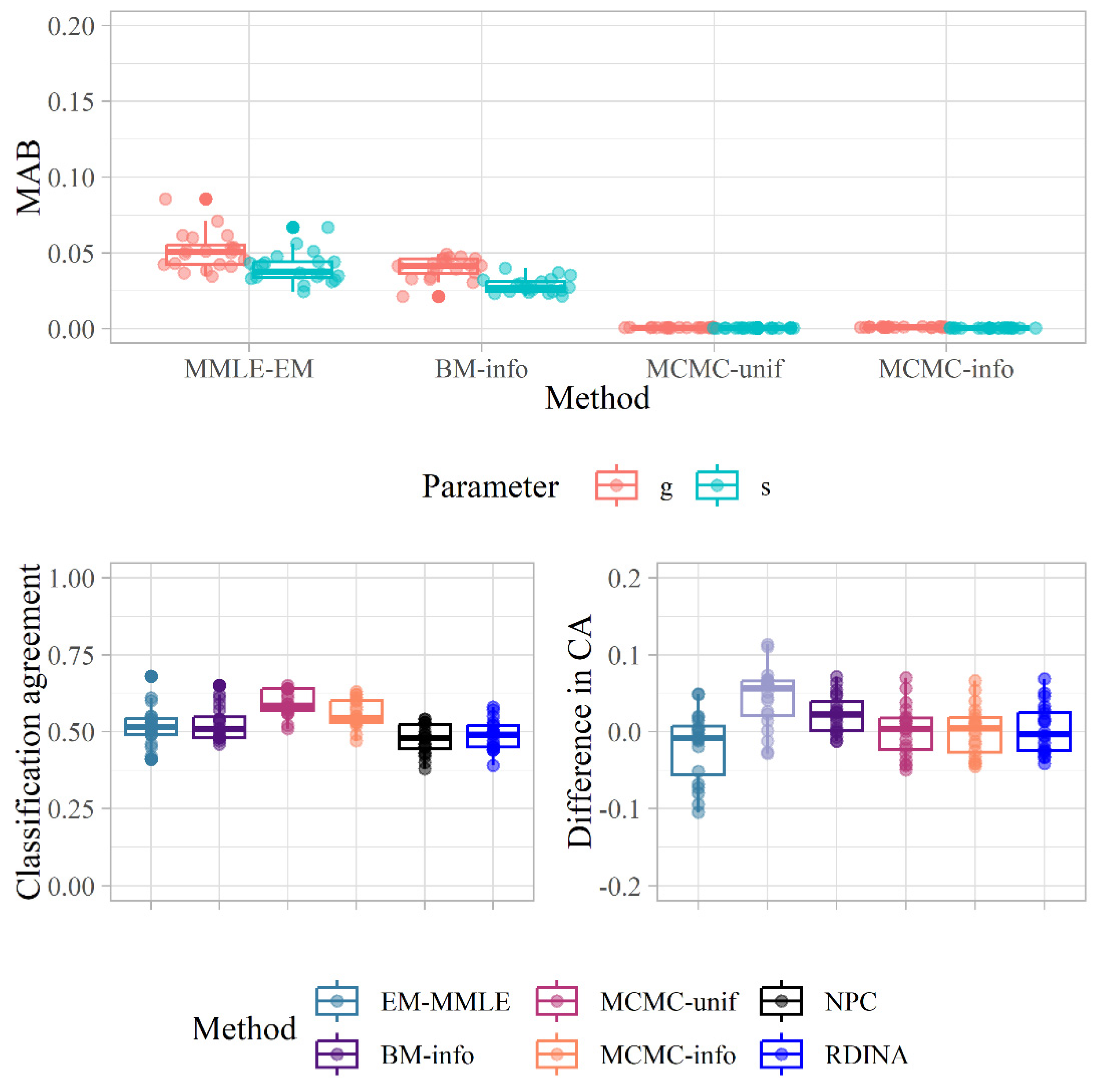
The same analyses were conducted on the empirical data, which are exhibited in Table 3. This time, the values reported reflects the average difference between the estimates in the total sample size of 536 participants and those obtained in the randomly selected sample of 100 examinees. The mean of the 20 replicas is presented and the complete distribution is shown in Figure 3.
The MCMC procedures were the ones that offered the most similar item parameters on average, with the average difference being practically zero. The method leading to the greatest differences in MAB was MMLE-EM (0.051 and 0.040 for guessing and slip, respectively), followed by BM-info (0.040 and 0.029 for guessing and slip, respectively). Regarding the similarity between the classifications performed with calibration in both samples, it was highest for MCMC-unif (0.593) followed by MCMC-info (0.558). MMLE-EM was the most divergent in results (0.519), with BM-info in second place (0.528) for the DINA model estimates. Notably, NPC and RDINA offered even more divergent rankings than those offered by MMLE-EM (0.476 and 0.487, respectively). With respect to reliability estimation, there were no major differences, with the estimator for samples of 100 generally coinciding with that obtained with the full sample. The biggest difference was for MMLE-EM with MI (0.044) which this time offered, on average, slightly higher values in the small samples.
Overall, the estimation times were similar to the ones obtained in the simulation study. The MMLE-EM, BM-info, NPC, and R-DINA were generally estimated in less than a second. MCMC-info and MCMC-unif performed at 28 min for 100 and 536 individuals.
4. Discussion
In response to the growing field of the use of CDMs for smaller sample sizes, this paper examined various estimation methods of the DINA model comparing small and large sample sizes with simulated and empirical data, namely MMLE-EM estimation, MCMC estimation, and BM estimation. The NPC method and R-DINA model were also implemented to compare with the other methods, as these procedures were specifically designed for small sample scenarios. The results of the simulation study and the empirical data study show that, when the sample size was small (n = 100), the DINA model based on the MMLE-EM algorithm demonstrated a higher bias in the item parameters that translated to worse attribute classifications and reliability estimates when the sample size was low; meanwhile, MCMC performed better overall. BM also performed better than MMLE-EM in all the metrics considered. There were no differences between the procedures when the sample size was large (n = 2000). As expected, the Bayesian procedures using a prior distribution compatible with the true parameters performed better. It should be noted that it was predefined to assume a prior distribution [β(5, 25)] centered at 0.16 when in reality guessing and slips of 0.20 were simulated. Better performance would be expected by employing a prior distribution fully compatible with the generated data (i.e., with the maximum at 0.20 and lower variance). We wanted to reflect the fact that researchers may have some knowledge about the characteristics of their items, but with some margin of error. Even so, we found that MCMC without prior information (i.e., using a flat distribution) performed better than MMLE-EM. That is, if no prior knowledge is available, MCMC may be still a better alternative to MMLE-EM.
In both the simulation and the real data study, R-DINA generally had a good performance in terms of classification accuracy and reliability estimation, surpassing or equaling many of the estimation methods for DINA. However, it should be noted that this is a very restrictive model, operating under the constraint guessing equals slip for all items. In the simulation, this was true, thus favoring a good performance of R-DINA. Note however that the performance of R-DINA and NPC in terms of classification agreement in the simulation study was worse compared to the estimation of the DINA model. As argued in the Materials and Methods section, this is to be expected considering the variability in the estimated guessing and slip parameters and the results of the relative fit indices, which showed a preference for the DINA model. Exploring this prior to interpreting any model will therefore prove crucial. Although Nájera et al. (in press) [36] have found that R-DINA can perform better than DINA even when this constraint is violated, in low sample conditions where the estimation of the DINA model is very noisy (i.e., very small sample size, poor item quality), we want to emphasize that it is necessary that, before interpreting the output of R-DINA, an evaluation of its fit to the data and the relative fit with respect to the DINA model is carried out. As noted in the results, when appropriate to use, R-DINA provides accurate classifications, such as nonparametric methods, and an unbiased estimate of reliability.
It should be observed from the results that the guessing parameter estimation is more precise than the slip parameter. This can be explained because we have more participants from whom to estimate guessing and fewer people to estimate slip from in the DINA model, resulting in a more precise estimation of guessing. As is also evidenced from the results, a correct estimation of item parameters such as guessing and slip is fundamental for retrieving precise classifications and reliability estimates.
As with any simulation study, its results are generalizable to the extent that the simulated conditions represent reality. Although an empirical study is also presented and the levels of the factors considered were set at values congruent with the empirical studies available to date, some comments can be made regarding the design to motivate future research on the topic. First, in the present study we focused on the DINA model because it is the most used model according to the review by Sessoms and Henson (2018) [8] and it is easier to interpret. Nonetheless, we recommend exploring the difference in performance among the estimation procedures for more complex models such as the G-DINA model (e.g., [53]). The estimation of the DINA model is simpler as it has a smaller number of parameters to estimate. Under more complex models, the differences between estimation methods can be expected to become larger. That is, the results reported here may represent a downward estimate of the differences between methods. This was precisely the objective of the article: to check whether there are differences under low or intermediate conditions of number of attributes, items, and model complexity.
Second, the differences in computation time were large. The method with the best performance (MCMC) was also the slowest. In situations of large sample size where no differences in performance between estimation procedures can be expected, MMLE-EM, which is very fast, can be preferred. Nonetheless, it is worth pointing out that a total of 5000 iterations, 1000 of them being burn-in, were conducted to assure model convergence and stability. Nonetheless, this could be achieved with a lessened number of iterations, significantly reducing the computation time. A pilot study should be conducted to evaluate if the parameter and estimations differ notably. Other researchers are also developing algorithms to reduce the computational cost of MCMC (e.g., [54]). Regarding another decision of the researcher, it should be kept in mind that Bayesian procedures allow the selection of prior distributions that vary in degree of informativeness. It is important that this decision is not arbitrary but based on substantive criteria or actual prior information (e.g., how difficult a topic is, how a similar item worked in the past).
Finally, the number of samples extracted in the empirical study was relatively small (i.e., 20). Although examination of the distribution of the results obtained (see Figure 3) shows that the conclusions drawn will be stable, the number of replicates could be increased for greater precision in order to interpret the averages more carefully. In relation to the previous point, in order to achieve this, it would be convenient to examine ways to speed up the MCMC estimation.
5. Conclusions
This study finds that in large sample sizes the differences in performance between the estimation procedures are negligible, which leads to the conclusion that it does not matter which one is used and lower computational cost may be preferable. In addition, in the simulation study, it can be firmly judged that the DINA model can be recovered with very high precision in a small sample scenario because the results were identical, or differ in decimals, to those obtained with the true, generating model, which is the best estimation one could possibly have. Furthermore, the alternative estimation methods are preferred over MMLE-EM under these low sample-size conditions. Therefore, to obtain more accurate estimates of CDM parameters, it is advisable for practitioners to explore alternative estimation methods when dealing with small sample sizes.
Author Contributions
Conceptualization, M.A.S.; software, M.A.S. and S.E.; investigation, M.A.S., S.E., P.N., R.S.K. and R.V.-L.; writing—original draft preparation, M.A.S. and S.E.; writing—review and editing, M.A.S., S.E., P.N., R.S.K. and R.V.-L.; visualization, S.E.; supervision: M.A.S.; project administration, M.A.S.; funding acquisition, M.A.S. All authors have read and agreed to the published version of the manuscript.
Funding
This research was funded by Consejería de Ciencia, Universidades e Innovación of Comunidad de Madrid, Spain, through the Pluriannual Agreement with Universidad Autónoma de Madrid, grant number SI3/PJI/2021-00258.
Institutional Review Board Statement
Not applicable.
Informed Consent Statement
Not applicable.
Data Availability Statement
The R script and the data are available upon request to the corresponding author.
Acknowledgments
To those who have worked in the development of the R packages used and/or provided in the papers access to their estimation routines.
Conflicts of Interest
The authors declare no conflict of interest.
References
- Ren, H.; Xu, N.; Lin, Y.; Zhang, S.; Yang, T. Remedial teaching and learning from a cognitive diagnostic model perspective: Taking the data distribution characteristics as an example. Front. Psychol. 2021, 12, 628607. [Google Scholar] [CrossRef] [PubMed]
- Sorrel, M.A.; Abad, F.J.; Olea, J.; de la Torre, J.; Barrada, J.R. Inferential item-fit evaluation in cognitive diagnosis modeling. Appl. Psychol. Meas. 2017, 41, 614–631. [Google Scholar] [CrossRef] [PubMed]
- Tan, Z.; de la Torre, J.; Ma, W.; Huh, D.; Larimer, M.E.; Mun, E.Y. A tutorial on cognitive diagnosis modeling for characterizing mental health symptom profiles using existing item responses. Prev. Sci. 2022, 24, 480–492. [Google Scholar] [CrossRef] [PubMed]
- Templin, J.L.; Henson, R.A. Measurement of psychological disorders using cognitive diagnosis models. Psychol. Methods 2006, 11, 287–305. [Google Scholar] [CrossRef] [PubMed]
- Chen, J.; de la Torre, J. A general cognitive diagnosis model for expert-defined polytomous attributes. Appl. Psychol. Meas. 2013, 37, 419–437. [Google Scholar] [CrossRef]
- Ravand, H.; Baghaei, P. Diagnostic classification models: Recent developments, practical issues, and prospects. Int. J. Test. 2020, 20, 24–56. [Google Scholar] [CrossRef]
- Shi, Q.; Ma, W.; Robitzsch, A.; Sorrel, M.A.; Man, K. Cognitively diagnostic analysis using the G-DINA model in R. Psych 2021, 3, 812–835. [Google Scholar] [CrossRef]
- Sessoms, J.; Henson, R.A. Applications of diagnostic classification models: A literature review and critical commentary. Measurement 2018, 16, 1–17. [Google Scholar] [CrossRef]
- Junker, B.W.; Sijtsma, K. Cognitive assessment models with few assumptions, and connections with nonparametric item response theory. Appl. Psychol. Meas. 2001, 25, 258–272. [Google Scholar] [CrossRef]
- Tatsuoka, C. Data analytic methods for latent partially ordered classification models. J. R. Stat. Soc. Ser. C Appl. Stat. 2002, 51, 337–350. [Google Scholar] [CrossRef]
- De La Torre, J. The generalized DINA model framework. Psychometrika 2011, 76, 179–199. [Google Scholar] [CrossRef]
- Sorrel, M.A.; Abad, F.J.; Nájera, P. Improving accuracy and usage by correctly selecting: The effects of model selection in cognitive diagnosis computerized adaptive testing. Appl. Psychol. Meas. 2021, 45, 112–129. [Google Scholar] [CrossRef]
- de la Torre, J.; Minchen, N. Cognitively diagnostic assessments and the cognitive diagnosis model framework. Psicol. Educ. 2014, 20, 89–97. [Google Scholar] [CrossRef]
- Wu, H.M. Online individualised tutor for improving mathematics learning: A cognitive diagnostic model approach. Educ. Psychol. (Lond.) 2019, 39, 1218–1232. [Google Scholar] [CrossRef]
- Sanz, S.; Kreitchmann, R.S.; Nájera, P.; Moreno, J.D.; Martínez-Huertas, J.A.; Sorrel, M.A. FoCo: A Shiny app for formative assessment using cognitive diagnosis modeling. Psicol. Educ. 2023; in press. [Google Scholar]
- Li, F.; Cohen, A.; Bottge, B.; Templin, J. A latent transition analysis model for assessing change in cognitive skills. Educ. Psychol. Meas. 2016, 76, 181–204. [Google Scholar] [CrossRef]
- Sun, Y.; Suzuki, M. Diagnostic assessment for improving teaching practice. Int. J. Inf. Educ. Technol. 2013, 3, 607–610. [Google Scholar] [CrossRef]
- Ma, W.; de la Torre, J. GDINA: An R package for cognitive diagnosis modeling. J. Stat. Softw. 2020, 93, 1–26. [Google Scholar] [CrossRef]
- Ma, W.; de la Torre, J. GDINA: The Generalized DINA Model Framework. R Package Version 2.9.3. 2022. Available online: https://CRAN.R-project.org/package=GDINA (accessed on 1 March 2023).
- George, A.C.; Robitzsch, A.; Kiefer, T.; Groß, J.; Ünlü, A. The R package CDM for cognitive diagnosis models. J. Stat. Softw. 2016, 74, 1–24. [Google Scholar] [CrossRef]
- Robitzsch, A.; Kiefer, T.; George, A.C.; Ünlü, A. CDM: Cognitive Diagnosis Modeling. R Package Version 8.2-6. 2022. Available online: https://CRAN.R-project.org/package=CDM (accessed on 1 March 2023).
- Nájera, P.; Abad, F.J.; Sorrel, M.A. Determining the number of attributes in cognitive diagnosis modeling. Front. Psychol. 2021, 12, 614470. [Google Scholar] [CrossRef]
- Nájera, P.; Sorrel, M.A.; Abad, F.J. cdmTools: Useful Tools for Cognitive Diagnosis Modeling. R Package Version 1.0.3. 2023. Available online: https://github.com/Pablo-Najera/cdmTools (accessed on 30 March 2023).
- Sorrel, M.A.; Nájera, P.; Abad, F.J. cdcatR: An R package for cognitive diagnostic computerized adaptive testing. Psych 2021, 3, 386–403. [Google Scholar] [CrossRef]
- Kreitchmann, R.S.; de la Torre, J.; Sorrel, M.A.; Nájera, P.; Abad, F.J. Improving reliability estimation in cognitive diagnosis modeling. Behav. Res. Methods, 2022; in press. [Google Scholar] [CrossRef] [PubMed]
- Yamaguchi, K. On the boundary problems in diagnostic classification models. Behaviormetrika 2023, 50, 399–429. [Google Scholar] [CrossRef]
- Culpepper, S.A. Bayesian estimation of the DINA model with Gibbs sampling. J. Educ. Behav. Stat. 2015, 40, 454–476. [Google Scholar] [CrossRef]
- Culpepper, S.A.; Hudson, A. An improved strategy for Bayesian estimation of the reduced reparametrized unified model. Appl. Psychol. Meas. 2018, 42, 99–115. [Google Scholar] [CrossRef]
- van Ravenzwaaij, D.; Cassey, P.; Brown, S.D. A simple introduction to Markov Chain Monte–Carlo sampling. Psychon. Bull. Rev. 2018, 25, 143–154. [Google Scholar] [CrossRef]
- Metropolis, N.; Rosenbluth, A.W.; Rosenbluth, M.N.; Teller, A.H.; Teller, E. Equations of state calculations by fast computing machines. J. Chem. Phys. 1953, 21, 1087–1091. [Google Scholar] [CrossRef]
- Kruschke, J.K. Doing Bayesian Data Analysis: A Tutorial with R, JAGS, and Stan, 2nd ed.; Academic Press: Cambridge, MA, USA, 2015. [Google Scholar]
- Plummer, M. JAGS Version 4.3.1 User Manual. 2015. Available online: http://sourceforge.net/projects/mcmc-jags/ (accessed on 1 March 2023).
- Stan Development Team. Stan Modeling Language Users Guide and Reference Manual, Version 2.32. 2022. Available online: https://mc-stan.org/users/documentation/ (accessed on 1 March 2023).
- Ma, W.; Jiang, Z. Estimating cognitive diagnosis models in small samples: Bayes modal estimation and monotonic constraints. Appl. Psychol. Meas. 2021, 45, 95–111. [Google Scholar] [CrossRef]
- Chiu, C.Y.; Douglas, J. A nonparametric approach to cognitive diagnosis by proximity to ideal response patterns. J. Classif. 2013, 30, 225–250. [Google Scholar] [CrossRef]
- Nájera, P.; Abad, F.J.; Chiu, C.-Y.; Sorrel, M.A. A comprehensive cognitive diagnostic method for classroom-level assessments. J. Educ. Behav. Stat. 2023; in press. [Google Scholar] [CrossRef]
- Chiu, C.Y.; Sun, Y.; Bian, Y. Cognitive diagnosis for small educational programs: The general nonparametric classification method. Psychometrika 2018, 83, 355–375. [Google Scholar] [CrossRef]
- Paulsen, J.; Valdivia, D.S. Examining cognitive diagnostic modeling in classroom assessment conditions. J. Exp. Educ. 2022, 90, 916–933. [Google Scholar] [CrossRef]
- R Core Team. R: A Language and Environment for Statistical Computing. 2022. Available online: https://www.R-project.org/ (accessed on 1 March 2023).
- Sen, S.; Terzi, R. A comparison of software packages available for DINA model estimation. Appl. Psychol. Meas. 2020, 44, 150–164. [Google Scholar] [CrossRef]
- Rupp, A.A.; van Rijn, P.W. GDINA and CDM packages in R. Measurement 2018, 16, 71–77. [Google Scholar] [CrossRef]
- de la Torre, J. DINA model and parameter estimation: A didactic. J. Educ. Behav. Stat. 2009, 34, 115–130. [Google Scholar] [CrossRef]
- Su, Y.-S.; Yajima, M. R2jags: Using R to Run “JAGS”. R Package Version 0.5-7. 2015. Available online: http://CRAN.R-project.org/package=R2jags (accessed on 1 March 2023).
- Zhan, P.; Jiao, H.; Man, K.; Wang, L. Using JAGS for Bayesian cognitive diagnosis modeling: A tutorial. J. Educ. Behav. Stat. 2019, 44, 473–503. [Google Scholar] [CrossRef]
- Lee, S.Y. DINA Model with Independent Attributes. 2016. Available online: http://mc-stan.org/documentation/case-studies/dina_independent.html (accessed on 1 March 2023).
- Stan Development Team. RStan: The R Interface to Stan. R Package Version 2.21.8. 2023. Available online: https://mc-stan.org/ (accessed on 1 March 2023).
- Zheng, Y.; Chiu, C. NPCD: Nonparametric Methods for Cognitive Diagnosis. R Package Version 1.0-11. 2019. Available online: https://CRAN.R-project.org/package=NPCD (accessed on 1 March 2023).
- Gu, Y.; Xu, G. The sufficient and necessary condition for the identifiability and estimability of the DINA model. Psychometrika 2019, 84, 468–483. [Google Scholar] [CrossRef]
- Sorrel, M.A.; de la Torre, J.; Abad, F.J.; Olea, J. Two-step likelihood ratio test for item-level model comparison in cognitive diagnosis models. Methodology 2017, 13, 39–47. [Google Scholar] [CrossRef]
- Chen, J.; de la Torre, J.; Zhang, Z. Relative and absolute fit evaluation in cognitive diagnosis modeling. J. Educ. Meas. 2013, 50, 123–140. [Google Scholar] [CrossRef]
- DeCarlo, L.T. On the analysis of fraction subtraction data: The DINA model, classification, latent class sizes, and the Q-matrix. Appl. Psychol. Meas. 2011, 35, 8–26. [Google Scholar] [CrossRef]
- Iaconangelo, C. Uses of Classification Error Probabilities in the Three-Step Approach to Estimating Cognitive Diagnosis Models. Ph.D. Thesis, Rutgers University, New Brunswick, NJ, USA, 2017. [Google Scholar]
- Jiang, Z.; Carter, R. Using Hamiltonian Monte Carlo to estimate the log-linear cognitive diagnosis model via Stan. Behav. Res. Methods 2018, 51, 651–662. [Google Scholar] [CrossRef] [PubMed]
- Yamaguchi, K.; Templin, J. A Gibbs sampling algorithm with monotonicity constraints for diagnostic classification models. J. Classif. 2022, 39, 24–54. [Google Scholar] [CrossRef]
Figure 1.
DINA MMLE-EM item parameter estimates for items 9 ( = 0.29 and = 0.25) and 12 ( = 0.13 and = 0.04) of the fraction–subtraction dataset [10].
Figure 1.
DINA MMLE-EM item parameter estimates for items 9 ( = 0.29 and = 0.25) and 12 ( = 0.13 and = 0.04) of the fraction–subtraction dataset [10].

Figure 2.
Relationship between mean absolute bias of the item parameters and proportion of correctly classified attribute vectors and reliability bias for simulated data.
Figure 2.
Relationship between mean absolute bias of the item parameters and proportion of correctly classified attribute vectors and reliability bias for simulated data.

Figure 3.
Representation of the mean absolute bias of guessing and slip (MAB), classification agreement, and difference in estimated classification accuracy (CA) across the 20 replications of 100 cases compared to the results complete fraction–subtraction dataset.
Figure 3.
Representation of the mean absolute bias of guessing and slip (MAB), classification agreement, and difference in estimated classification accuracy (CA) across the 20 replications of 100 cases compared to the results complete fraction–subtraction dataset.


Table 1.
Estimated DINA item parameters for the fraction–subtraction dataset.
| Guessing Parameter | Slip Parameter | |||||||
|---|---|---|---|---|---|---|---|---|
| Item | MMLE-EM | BM-Info | MCMC-Unif | MCMC-Info | MMLE-EM | BM-Info | MCMC-Unif | MCMC-Info |
| 1 | 0.030 | 0.049 | 0.045 | 0.065 | 0.089 | 0.094 | 0.078 | 0.085 |
| 2 | 0.016 | 0.041 | 0.025 | 0.048 | 0.041 | 0.045 | 0.040 | 0.045 |
| 3 | 0.000 | 0.021 | 0.008 | 0.026 | 0.134 | 0.127 | 0.132 | 0.124 |
| 4 | 0.224 | 0.218 | 0.236 | 0.228 | 0.110 | 0.110 | 0.111 | 0.112 |
| 5 | 0.301 | 0.287 | 0.310 | 0.292 | 0.172 | 0.167 | 0.153 | 0.152 |
| 6 | 0.095 | 0.116 | 0.198 | 0.176 | 0.044 | 0.047 | 0.038 | 0.045 |
| 7 | 0.025 | 0.041 | 0.035 | 0.049 | 0.197 | 0.182 | 0.201 | 0.184 |
| 8 | 0.444 | 0.376 | 0.434 | 0.370 | 0.182 | 0.176 | 0.164 | 0.163 |
| 9 | 0.288 | 0.212 | 0.237 | 0.182 | 0.247 | 0.238 | 0.248 | 0.237 |
| 10 | 0.029 | 0.041 | 0.035 | 0.047 | 0.214 | 0.203 | 0.193 | 0.187 |
| 11 | 0.066 | 0.074 | 0.067 | 0.076 | 0.082 | 0.083 | 0.084 | 0.086 |
| 12 | 0.127 | 0.140 | 0.265 | 0.233 | 0.041 | 0.050 | 0.038 | 0.048 |
| 13 | 0.013 | 0.026 | 0.017 | 0.030 | 0.335 | 0.312 | 0.336 | 0.313 |
| 14 | 0.062 | 0.087 | 0.162 | 0.146 | 0.061 | 0.066 | 0.045 | 0.056 |
| 15 | 0.031 | 0.053 | 0.032 | 0.055 | 0.105 | 0.103 | 0.113 | 0.112 |
| 16 | 0.109 | 0.118 | 0.184 | 0.163 | 0.111 | 0.110 | 0.092 | 0.098 |
| 17 | 0.038 | 0.051 | 0.044 | 0.054 | 0.138 | 0.136 | 0.142 | 0.139 |
| 18 | 0.119 | 0.124 | 0.130 | 0.133 | 0.138 | 0.136 | 0.135 | 0.133 |
| 19 | 0.022 | 0.034 | 0.026 | 0.037 | 0.240 | 0.221 | 0.235 | 0.214 |
| 20 | 0.013 | 0.027 | 0.020 | 0.031 | 0.157 | 0.154 | 0.144 | 0.144 |
Table 2.
Average values across conditions for mean absolute bias of the item parameters, proportion of correctly classified attribute vectors, and reliability bias of the simulated data.
Table 2.
Average values across conditions for mean absolute bias of the item parameters, proportion of correctly classified attribute vectors, and reliability bias of the simulated data.
| Method | MAB (g/s) | PCV | Reliability Bias | |||
|---|---|---|---|---|---|---|
| n = 100 | n = 2000 | n = 100 | n = 2000 | n = 100 | n = 2000 | |
| MMLE-EM | 0.048/0.089 | 0.010/0.018 | 0.622 | 0.692 | 0.191 | 0.011 |
| MMLE-EM with MI | - | - | - | - | 0.000 | −0.003 |
| BM-info | 0.033/0.044 | 0.010/0.017 | 0.660 | 0.692 | 0.086 | 0.009 |
| MCMC-unif | 0.044/0.084 | 0.010/0.018 | 0.660 | 0.686 | 0.026 | 0.010 |
| MCMC-info | 0.029/0.033 | 0.010/0.017 | 0.688 | 0.687 | 0.041 | 0.013 |
| NPC | - | - | 0.692 | 0.692 | - | - |
| R-DINA | - | - | 0.690 | 0.691 | 0.002 | 0.000 |
| True, generating model | 0.692 | 0.692 | 0.001 | −0.001 | ||
Notes: The SD of MAB varies between 0.001 and 0.016. The SD of PCV under the n = 100 sample condition varies between 0.047 and 0.054 and is around 0.010 under the n = 2000 sample conditions. The SD of reliability bias under the n = 100 sample condition varies between 0.035 and 0.056 and is around 0.010 under the n = 2000 sample conditions.
Table 3.
Average values across 20 replications for mean absolute bias of guessing and slip, classification agreement, and difference in estimated classification accuracy.
Table 3.
Average values across 20 replications for mean absolute bias of guessing and slip, classification agreement, and difference in estimated classification accuracy.
| Method | MAB (g/s) | Classification Agreement | Difference in Estimated Classification Accuracy |
|---|---|---|---|
| MMLE-EM | 0.051/0.040 | 0.519 | −0.019 |
| MMLE-EM with MI | - | - | 0.044 |
| BM-info | 0.040/0.029 | 0.528 | 0.023 |
| MCMC-unif | 0.001/0.001 | 0.593 | 0.001 |
| MCMC-info | 0.001/0.001 | 0.558 | 0.001 |
| NPC | - | 0.476 | - |
| R-DINA | - | 0.487 | 0.003 |
Notes: The results presented are the difference between the 536 and the 100 samples. SD were generally very low, with 0 being the smallest and 0.064 the greatest.
Disclaimer/Publisher’s Note: The statements, opinions and data contained in all publications are solely those of the individual author(s) and contributor(s) and not of MDPI and/or the editor(s). MDPI and/or the editor(s) disclaim responsibility for any injury to people or property resulting from any ideas, methods, instructions or products referred to in the content. |
© 2023 by the authors. Licensee MDPI, Basel, Switzerland. This article is an open access article distributed under the terms and conditions of the Creative Commons Attribution (CC BY) license (https://creativecommons.org/licenses/by/4.0/).
Share and Cite
MDPI and ACS Style
Sorrel, M.A.; Escudero, S.; Nájera, P.; Kreitchmann, R.S.; Vázquez-Lira, R. Exploring Approaches for Estimating Parameters in Cognitive Diagnosis Models with Small Sample Sizes. Psych 2023, 5, 336-349. https://doi.org/10.3390/psych5020023
AMA Style
Sorrel MA, Escudero S, Nájera P, Kreitchmann RS, Vázquez-Lira R. Exploring Approaches for Estimating Parameters in Cognitive Diagnosis Models with Small Sample Sizes. Psych. 2023; 5(2):336-349. https://doi.org/10.3390/psych5020023
Chicago/Turabian StyleSorrel, Miguel A., Scarlett Escudero, Pablo Nájera, Rodrigo S. Kreitchmann, and Ramsés Vázquez-Lira. 2023. "Exploring Approaches for Estimating Parameters in Cognitive Diagnosis Models with Small Sample Sizes" Psych 5, no. 2: 336-349. https://doi.org/10.3390/psych5020023