1. Introduction
Human gait is a complex phenomenon of locomotion that develops as a child grows and learns to move forward using the cyclic movement of the lower limbs [
1]. It is a distinguishable biological feature of a human being. Any deviation from a normal gait pattern can be due to old age or maybe a sign indicating the onset of neurological diseases such as Parkinson’s [
2], ALS [
3], cerebral palsy [
4], COVID-19 [
5], stroke [
6], and vertigo [
7]. The study of gait is not only relevant to medical applications but also extends to other fields [
8].
Currently, the technology for gait analysis uses a combined movement capture system with non-wearable force platforms. However, this state-of-the-art technology is expensive due to the optical equipment required and is limited by the need for a lab setup and constrained environment [
1]. As a result, the cost of developing, installing, and maintaining these complex systems can be a barrier to their commercialization and practical use. In contrast, the use of micro-electro mechanical systems (MEMS) technology, especially in the form of inexpensive Internet of Things (IoT) devices equipped with accelerometers and gyroscopes, has become widely used for gait data acquisition, analysis, and prediction [
9,
10,
11].
These wearable devices are typically attached to the ankles and waist to capture accelerometer and gyroscope signals, which are used to identify the gait cycle and movement of a single limb, distinguishing between the stance and swing phase. The real-time classification of abnormal human gait using these devices can be used to develop control devices for orthotics and prosthetics, monitor rehabilitation, and create fall detection systems for elderly individuals [
8].
This paper presents a novel device that captures and preprocesses gyroscope and acceleration signals from both legs using Euler angles and a Madgwick orientation filter. It utilizes the various variations of a CNN neural network, a custom data logger, and deep learning techniques to find the optimal model. The final model is then exported and optimized for use on resource-constrained devices such as ARM for inference.
2. Related Work
The revolution in connected devices has proven to be a technological advancement for the future. Edge AI offers an alternative to traditional cloud computing and enables new types of applications to be as close as possible to end-users and data sources [
12]. This is especially useful for running machine learning (ML) inferences as close to the sensor that produces the data as possible, as the edge device does not require constant connectivity for data transmission and is energy-efficient [
13]. Typically, an IoT device connects to a designated gateway via radio and sends data to the cloud for further processing. However, executing instructions at the edge can be more energy-efficient than transmitting data [
13]. This paragraph describes existing techniques for activity recognition using inertial measurement unit (IMU) sensors, enabling TinyML, and recent trends in TinyML for human activity recognition (HAR).
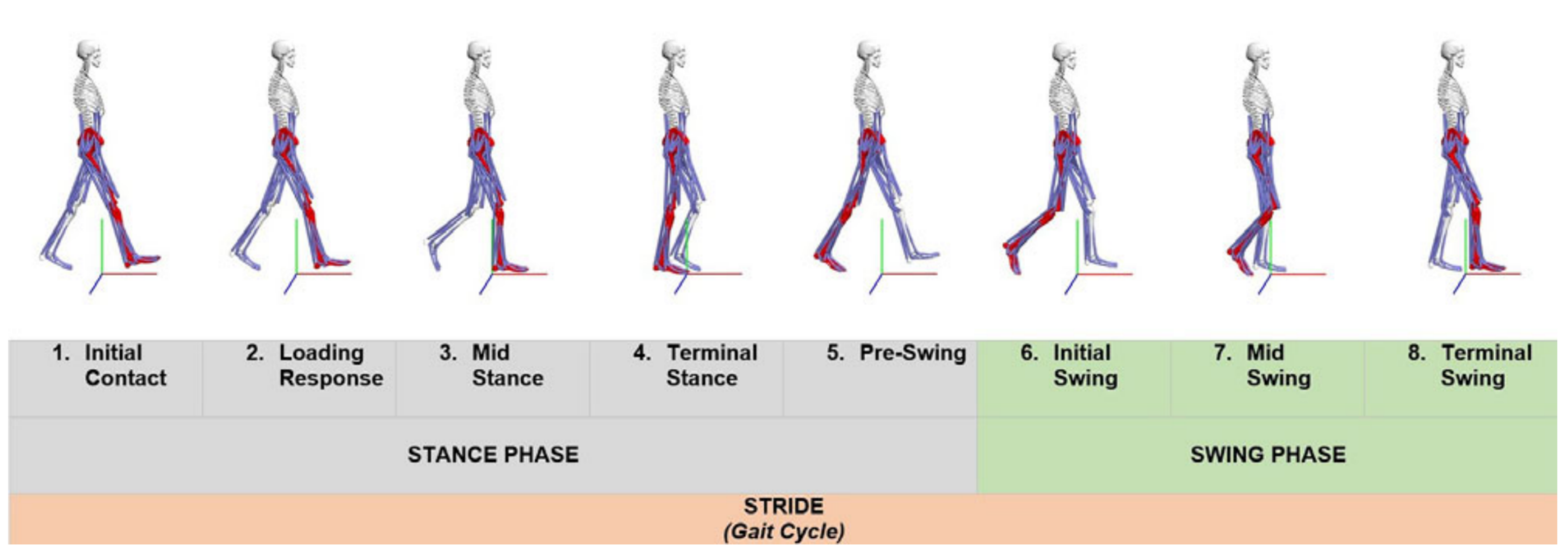
The action of bipedal and biphasic forward propulsion of the center of gravity of the human body, known as human gait, consists of two principal phases: the swing and stance phases. These phases are also divided into four sub-phases for the stance phase and three sub-phases for the swing phase, as shown in
Figure 1. The study of human movement (human gait analysis) has been extensively studied and researched over the past decade [
8], leading to the development of numerous devices to detect abnormalities in these patterns.
Firstly, Mantyjarvi et al. in [
15] attempted to identify gait patterns with IMU sensors and devise a device by capturing standard gait patterns using IMU data. The data consist of subjects walking at a fast, regular, and slow pace; these data are then correlated with a standard existing walking pattern to detect abnormalities. The study used histogram statistics, fast Fourier transform (FFT) coefficients, and correlation to generate a model and compare it to a standard and regular walking pattern. Gait analysis can be characterized as a biometric signal as every person’s walking pattern is different.
Secondly, Gao et al. and Patil et al. in [
16,
17] used the ML approach to address the nonlinear and complex problem. In [
17], Patil et al. also utilized K nearest neighbor, support vector machine, extreme learning machines, and multi-layer perceptrons (MLP) for abnormal gait classification. Their process included data acquisition, data smoothing, dimension reduction, feature selection, and classification that allowed them to obtain a classification accuracy of 85%, 90%, 93%, and 96% using KNN, MLPs, ELM, and SVM, respectively. They found that MLP had the worst performance while KNN had the best, with an inference time of 0.02 s on a decent workstation during the inference of these models. Similarly, Gao et al. in [
16] combined long short-term memory and CNN to classify gait patterns such as hemiplegic, tiptoe, and cross-threshold gait pattern detection using the IMU sensor and Euler angle. The study primarily investigated the different overlapping window lengths, the use of simple CNN networks only, and the accuracy of these models in resource-constrained devices.
Finally, a comprehensive survey study of human gait-based AI applications [
8] introduced the term smart gait (SG). The study discussed the applications and challenges faced by SG. The preliminary study of the survey was to identify and provide future areas of application for using ML in gait research. The application areas include gait phase detection, gait abnormality detection (stroke, neurological disease, Parkinson’s disease), human posture estimation, localization for simultaneous localization and mapping, individual identification, physical mobility, and fall risk assessment. Most studies were performed in controlled environments such as watching a smiley on the wall, performing a gait activity, and walking on a treadmill to collect data. The survey concludes that there is a gap to fulfill the space between the controlled and the real-life setup.
One of the challenges in this field of research is the collection of pathological gait data from actual patients, as most analyses are typically conducted on normal subjects. Additionally, the commercialization of these products requires government approvals and food and drug administration certification, as well as the acceptance and adoption by doctors and therapists. To be successful, the product development life-cycle cost must be practical and affordable to overcome the barrier of adoption. Despite these challenges, AI-based gait research is a rapidly growing area of investigation, with ongoing efforts to develop nonlinear solutions for abnormality gait detection. However, much of the current research and development in this area focuses on larger computing devices, and relatively little research has been devoted to targeting tiny, resource-constrained devices. This study aims to fill that gap by investigating the use of such devices for abnormal gait detection
Main Contributions
This paper introduces a cutting-edge context-aware IoT device designed to identify and analyze irregular gait patterns. Utilizing gyroscope and acceleration signals from both legs, the device preprocesses the signals and employs the Madgwick orientation filter to calculate Euler angles. With the use of various CNN models and a custom data logger, the device generates overlapping datasets for multiple data channels and employs deep learning techniques to determine the optimal model, which is then exported to a format suitable for ARM to run the inference process. To the best of our knowledge, this is a first-of-its-kind solution in the field.
The following sub-objectives are required as an essential step toward the main contributions:
To make a data logger device to capture gait patterns using a wearable device on multiple human subjects.
To collect, split, and train an ML model to classify various gait patterns by employing the use of an IMU sensor.
To compress the ML model using post-training quantization to reduce the memory footprint.
To deploy the ML model and inference from an ARM chip.
To evaluate the model using classification accuracy, precision, recall, and F1-score to determine the best model from overlapping datasets.
To evaluate the performance of the inference using execution time and throughput for the best model.
3. Methodology
The methodology section outlines the process for creating a novel device to capture human gait patterns from a defined group of subjects. The standard ML process, including data collection, preprocessing, model design, and deployment, was applied to address the problem. The section is structured into sub-sections to clarify the ML pipeline, from data acquisition to the ML model deployment on an ARM SoC. It also provides insight into the sophisticated architecture and technologies used to create a data logger that generates a dataset into multiple groups of overlapping windows to determine whether overlapping data improve performance in a simple CNN architecture. The ML training and testing process is described to create an efficient model, and the best model is then deployed on the microcontroller and evaluated using various classification metrics.
3.1. Data Acquisition
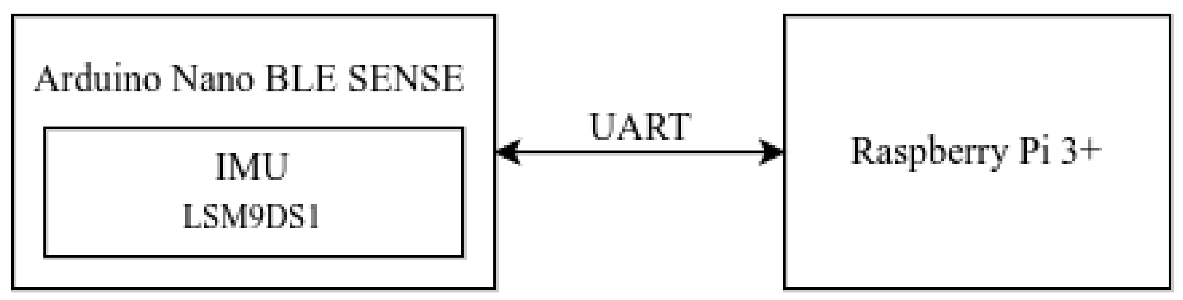
The quality of data plays an essential role in any supervised learning task. The data collection process is the most crucial and initial part. The data logger hardware, as shown in
Figure 2, makes use of an IoT development device called Arduino Nano Bluetooth Low Energy (BLE) Sense [
18] connected with a Raspberry Pi. This enables the Arduino board to receive data or instructions from a nearby device or sensor using the BLE, which is one of the most widely applicable low-power connectivity standards. The two devices communicate with each other using universal asynchronous receiver-transmitter (UART) communication. This protocol was chosen because it is easier to debug and establish a connection between the microcontroller and the Raspberry Pi. The data logger firmware and software used to preprocess, transform, and save the collected data in the desired file format on the Raspberry Pi is discussed as follows:
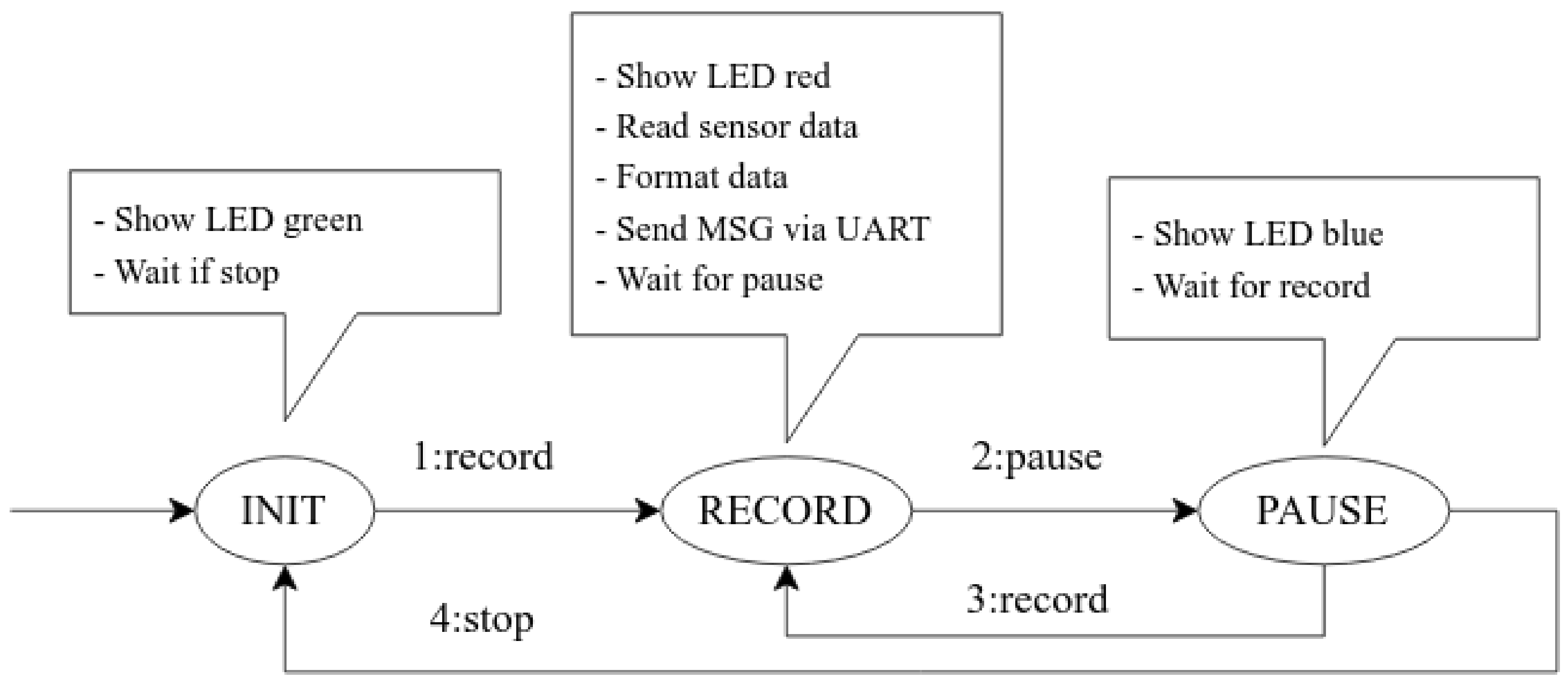
The data logger captures labeled datasets similarly to a video recorder, with software states of
INIT,
RECORD, and
PAUSE, as shown in
Figure 3. This allows participants to quickly wear the device, walk for a few minutes, and easily capture all the gait data. Once a connection is established with the parent controller and all necessary sensors are initialized, the data logger is in the
INIT state. State transition occurs when a peripheral device, such as a laptop or phone, sends a fixed message. The data are in the format “action:payload” and when a peripheral device sends “2:record”, the microcontroller transitions the status from led to red, read sensor data, constructs a payload in the desired format, and sends the data via UART. Using a serial connection allows for the fast capture of the data as it is generated at the highest baud rate to capture the nuances of the signals produced by the accelerometer.
Figure 3 shows more details of the working mechanism and state transition written in C++ language, which is deployed onto the microcontroller.
Figure 4 is written in general purpose high-level language, NodeJs, and consists of a serial listener, event emitter, application server, HTTP server for static frontend files, sockets for client communication, and a database for storing subject details such as name, age, and height. The gait logger and data logger server are serially connected, while the client application and server are connected using TCP/IP. The event emitter API is used to facilitate interprocess communication between the serial listener and the application server. The application server formats the captured data into overlapping windows and saves it in a file structure.
The data logger was constructed based on the hardware and software architecture described above and was used to collect a set of three pathological gaits and two standard human activity datasets, as shown in
Table 1. Two GAIT logger hardware devices were attached to both legs of a human subject. The participant was asked to carry out these five motions, and the data logger captured the associated data and saved it in a database for training purposes.
The gait logger software is designed to immediately convert received data into the appropriate dataset, requiring less preprocessing to format the data for training. The software creates overlapping datasets comprising 6 channels of acceleration data and 3 channels of Euler angles. For each data collection session, the software generates overlapping datasets as well. Overlapping windows with an interval of are chosen, where . The purpose of generating overlapping datasets at the same time is to facilitate the training and testing of the dataset and to validate whether overlapping window data has an impact on the performance of the model inference process.
3.2. Preprocess and Data Augmentation
Some preprocessing is required to augment the data based on the sensor’s limitation. Hence, the data from different sensors are normalized against the full specification of the sensor limits. The normalization of the accelerometer data point is given by
where the sensor value for the part LSM9DS1 [
19] sensor varies in any of the
x,
y, and
z direction from
to
. Similarly, the normalization of gyroscope values is carried out by
where the gyroscope sensor value in any
x,
y, and
z varies from
to
degrees per second (DPS). The data are shifted towards the mean before being sent into the deep learning network as suggested in [
20].
The 9DoF IMU LSM9DS1 is a system-in-package with a 3-axis accelerometer, 3-axis magnetometer, and 3-axis gyroscope. It has a maximum sampling frequency of 104 Hz for the accelerometer and gyroscope. This frequency is chosen based on the Nyquist criteria and the maximum possible frequency for human movement, which is around 8.5 Hz, as mentioned in the work by Qiao et al.’s [
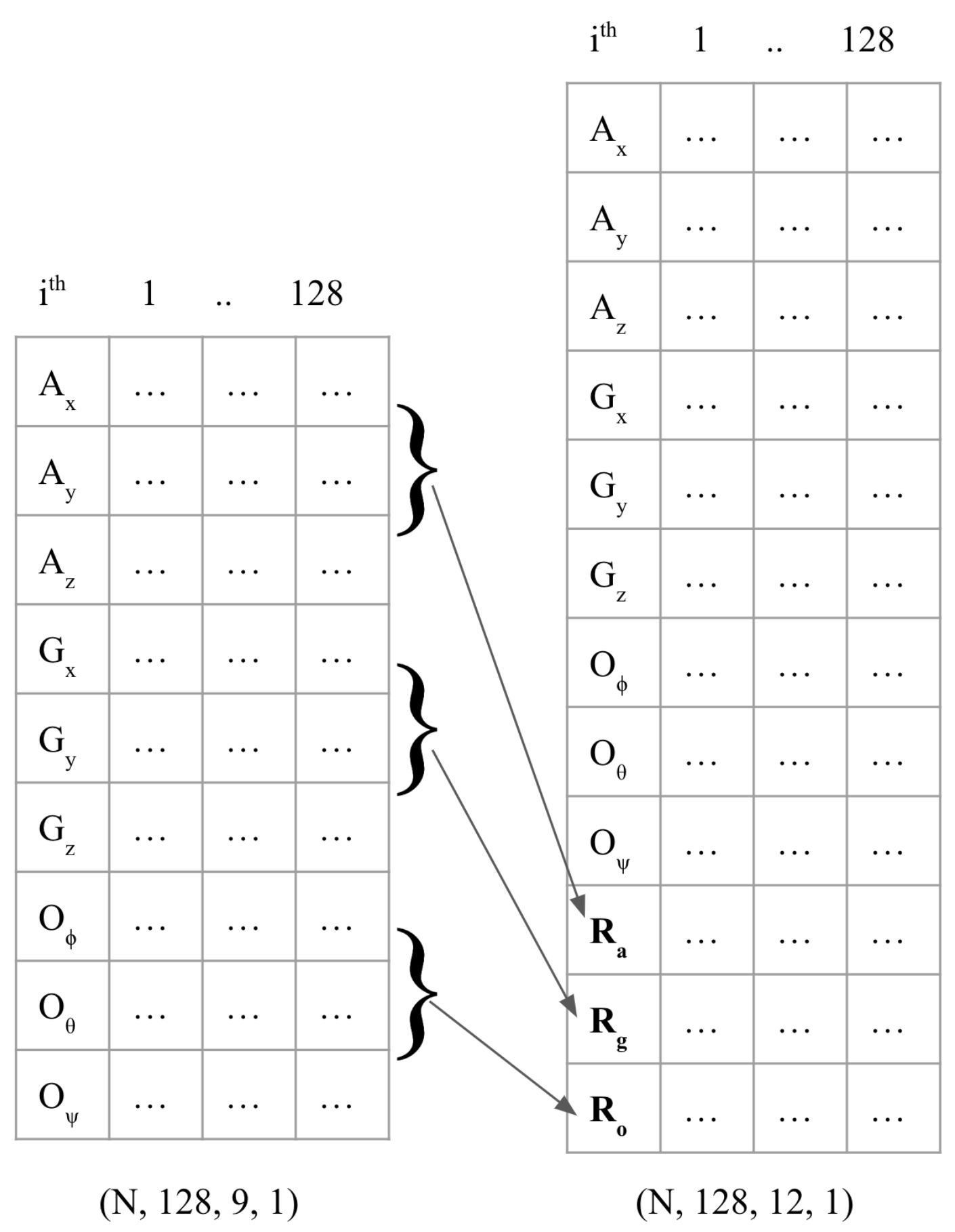
21]. To further aid the CNN model in extracting features, the data are augmented with the resultant accelerometer, gyroscope, and orientation angle. This results in a vector of size
, appended to the original vector of size
as
where
,
, and
are the resultant vector of acceleration, gyroscope, and orientation components. A data tensor of size
is constructed from
using the Equations (
3)–(
5) as shown in
Figure 5, and the dataset is further divided into the training, test, and validation sets.
A new tensor with 12 channels (i.e., the original nine channels plus three additional channels for the combined vectors) can potentially help the ML model learn more complex patterns and improve the generalization and robustness of the model by increasing the diversity of the training data, which leads to a better performance on new, unseen data.
3.3. Model Design
The output of the data acquisition procedure, as defined in
Section 3.1, yields datasets comprising various overlapping windows. A total of exactly 10 datasets are generated for each overlapping window. Each dataset is then trained using the Tensorflow Keras library, and the data are split based on the subject for testing on signals that are unknown to the deep-learning network. The training–test split involves selecting 80% of the data for training and 20% for testing, using a list of unique individuals. This process is repeated for all datasets with different overlapping windows. The datasets are mainly trained using three deep-learning architectures, where a simple architecture CNN is taken as the baseline, and the final architecture is obtained after fine-tuning the models, as described below:
3.3.1. CNN Architecture
The proposed CNN system architecture, which is summarized in
Table 2, uses 2D convolution (Conv 2D). It consists of a combination of accelerometer data, gyroscope data, and output from the Madgwick filter. The input data pass through an initial convolutional layer with a filter size of 64 and a kernel size of
, followed by a batch normalization layer and ReLU nonlinear activation. Then, an average-pooling layer is used to reduce the feature representation, followed by a dropout layer to reduce overfitting. This process is repeated with a kernel size of
, a filter size of 8, batch normalization, nonlinear ReLu activation, and average pooling of
. The output is then flattened and sent to a dense neural network layer with nonlinear ReLu activation, followed by a dropout layer to further reduce overfitting. Finally, the softmax layer computes the probability distribution over all five activity classes.
3.3.2. CNN-Statistics
The proposed method combines automatic feature extraction from CNN layers with statistical features. The statistical features are calculated for data-augmented channels with a window length of 128 and are concatenated with the output of the CNN network before being passed into a fully connected layer. The statistical features are only computed for the resultant vectors of acceleration, gyroscope, and orientation angles. A total of 12 statistical features (median, maximum, average, and standard deviation) are calculated from the resultant vectors of , , and as follows:
Mean value of resultant vectors : .
Standard deviation of resultant vectors : .
Maximum value of resultant vectors : .
Median value of resultant vectors average : .
The details of the architecture are shown in
Table 3 and described as follows.
This architecture was explored because the authors in [
20,
22] found a significant improvement in real-time accuracy inference using the combination of statistical features and CNN. Additionally, just a few input parameters were increased compared to the architecture defined in the ”CNN architecture” section. The proposed architecture in this paper combines a CNN network with signal statistic features to improve the performance of activity recognition. The process starts with an input shape of
, which is passed through a primary convolutional layer with a filter size of 64 and a kernel size of
. This is followed by a batch normalization layer and ReLU nonlinear activation. An average-pooling layer with a kernel size of
is applied to reduce the feature representation, and a dropout layer is used to prevent overfitting. The process continues with a Conv 2D layer, a batch normalization layer, a nonlinear ReLu activation, and an average pooling of
. In addition to this, 12 statistical features are computed from the resultant vectors of
,
, and
, and they are concatenated with the flattened output of the CNN network. The concatenated output is sent to a dense layer with ReLU activation, followed by a dropout layer and a softmax layer to compute the probability distribution over all five activity classes.
3.3.3. CNN-LSTM
An emerging approach to HAR activity recognition uses a combination of CNN and LSTM, as explored in this paper [
16,
23,
24]. The rationale behind proposing this approach is to improve the accuracy of the detection. The architecture mostly uses a time-distributed (TD) layer function provided by the Keras API to maintain temporal integrity for the LSTM layers. The TD layer expects 3D input, so the inputs were reshaped from a shape of
to
, with a window length of 128 decomposed into 4-time slices and 32 timesteps. The details of the architecture are shown in
Table 4 and described as follows.
The architecture uses a time-distributed (TD) layer function provided by the Keras API to maintain temporal integrity for the LSTM layers. An input shape of (
, 32, 12, 1) is used where a timestep of
= 4 is chosen, and reshaped from (128, 12, 1) as TD input requires a 3D shape. The input is passed onto distributed Conv2D layers with a filter size of 64 and a kernel size of 12, followed by TD batch normalization, TD ReLu activation, and TD dropout of 0.5 to avoid overfitting. The output from the convolutional layer is passed onto a GlobalAveragePooling2D layer [
25], TD flattened and sent to an LSTM layer, followed by a dropout layer to avoid overfitting. A fully connected dense layer is followed by the dropout output and finally, the softmax layer computes the probability distribution over all five activity classes.
3.4. Model Training
The goal was to create an optimized model for deployment on an ARM chip and inference using Raspberry Pi. The deep learning models were trained using the TensorFlow Keras API, with data trained for 100 epochs using categorical cross-entropy loss and an Adam optimizer with a learning rate of 0.0001. The model was fed with training data in batches of 128 and evaluated using accuracy as the metric. Callback methods were used to save model checkpoints using the minimum validation loss. A validation set of 20% from the training set was also used. The training was carried out on a machine with an Intel 8th generation CPU and Nvidia RTX 1050Ti 4GB graphics card.
3.5. Evaluation Metrics
The following performance metrics are used to evaluate our proposed model:
The accuracy is measured by the ratio of correctly predicted labels to the total number of predictions given by
where
tp (true positive) is the sum of successfully predicted classes,
tn (true negative) is the sum of valid classes that were negatively classified,
fn (false negative) is the sum of instances belonging to the positive class that were incorrectly predicted as negative, and
fp (false positive) is the sum of false predictions that should have been another class. Precision is calculated by taking the rate of correctly predicted classes over the total number of predictions given by
The
metric is the ratio calculated using the rate of a correctly predicted class over the fundamental data attributes of the class given by
The
metric computes a value that is a mixture of the precision and recall metrics given by
The average execution time would be helpful to compute the throughput of the above architecture run in a microcontroller. The unit of the execution time is in milliseconds (ms). The average execution time calculation, which is denoted by
, is calculated as
where
is a set of inferences taken at a certain interval of
t.
Throughput denoted by
is the reciprocal of estimated operations denoted by
computed over the execution time denoted by
, which is expressed as
4. Model Compression: Quantization
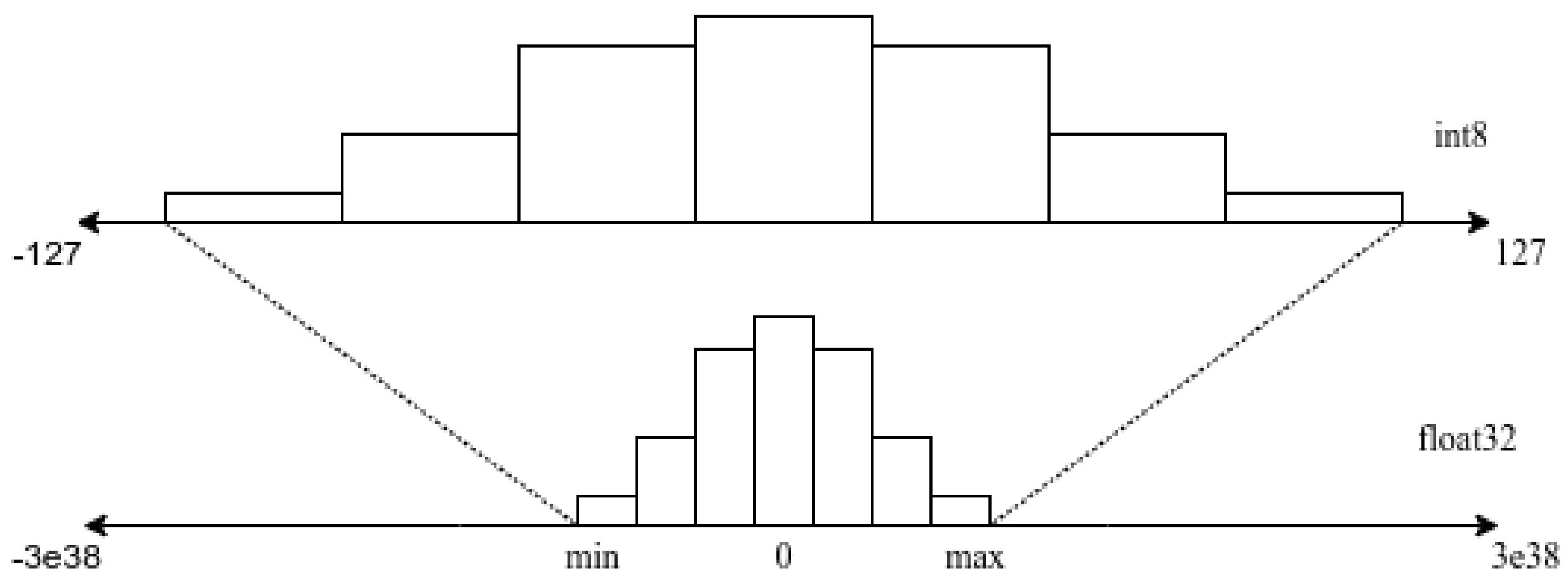
While performing summation and multiplication operations on single-precision floating-point format (sometimes called float32) values, the resultant operands, products, and accumulations are also float32. Quantization reduces the precision of operations by converting from higher representations of bits to lower primitive representations, for instance, from a 32-bit floating-point number to an 8-bit integer value. This process reduces the number of bits needed to designate weights. It is a probabilistic conversion based on the [min, max] range of the weight values shown in
Figure 6. For instance, one of the methods to achieve this is to first calculate the standard deviation and mean of all weights, choose the number of bits to assign, and then represent the integer portion to cover a range [
26]. Many other kinds of literature propose an effective way of quantization, such as linear quantization, log-based quantization, and k-means clustering.
Quantization is transforming an ML model into an approximated representation with available precision resources. The methodology enlists three types of quantization techniques available in TFLM API. These techniques are post-training quantization techniques, and their description is given as follows.
4.1. Reduced Float
The model parameters are converted from a 32-bit floating-point representation to a 16-bit word. The TFLM provides this conversion mechanism by simply checking some flags. It presents a size reduction and promotes faster inference with negligible accuracy loss.
4.2. Hybrid Quantization
Weight parameters are an 8-bit integer; the activations are a 16-bit float and biases as an 8-bit float. It includes both integer and floating-point computations. According to the documentation, it can reach a four-times reduction in model size, 10–50% faster inference for convolutional models, and 2–3× faster on fully connected layers.
4.3. Integer Quantization
The model compression is similar to hybrid quantization, but all the computations are performed in integers. However, it requires a small amount of data, approximately 100 samples, to represent floating-point values to int-8 representation.
To reduce the model size, the study implements integer quantization, where small samples of the dataset are fed into the quantization function and use the open APIs of the TensorFlow quantization technique to port the best model, as shown in
Section 3.4, and find the evaluation metrics shown in
Section 3.5.
4.4. Model Deployment
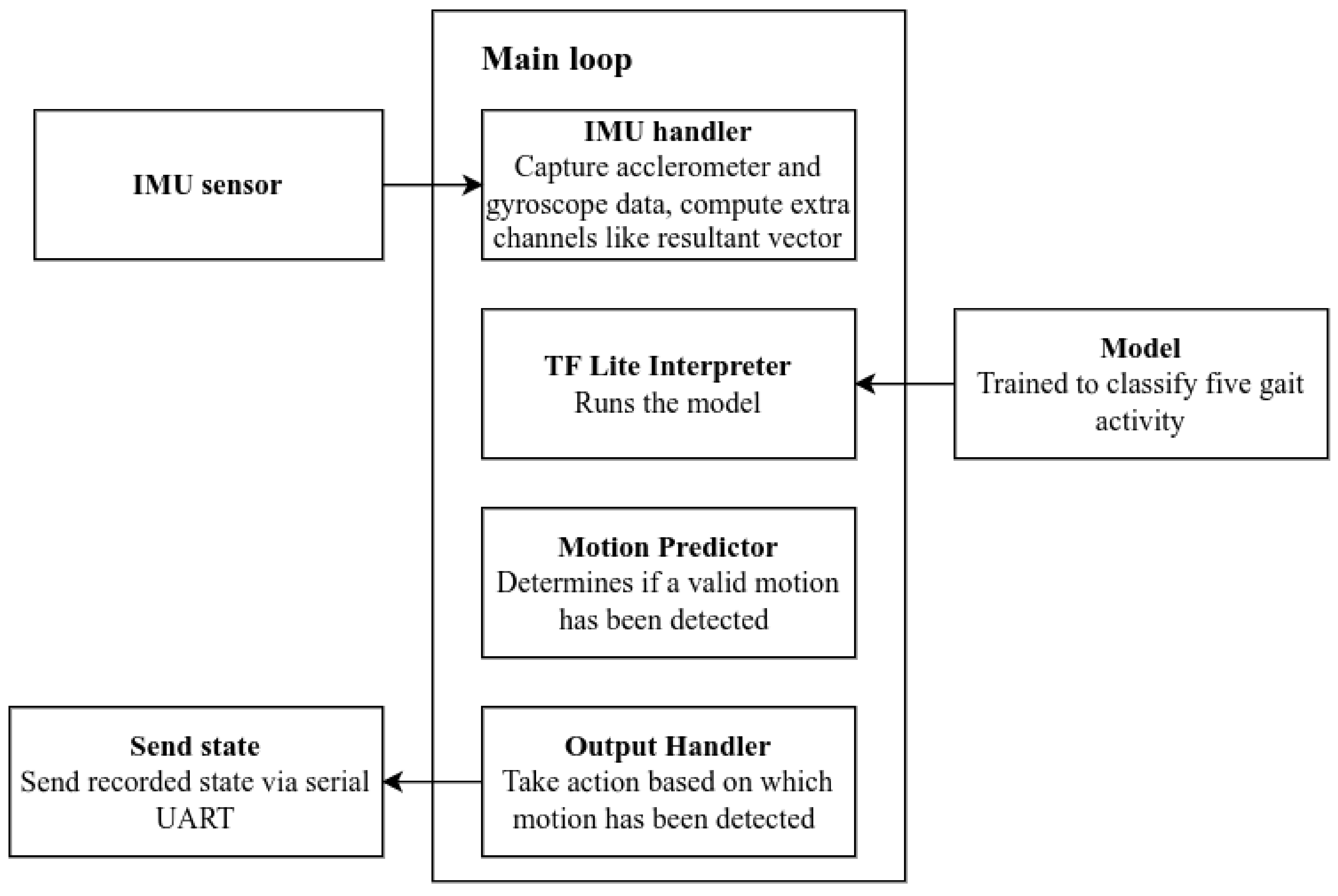
The best model was selected through the training and evaluation procedures defined previously. To accurately detect human gait patterns on a resource-constrained device, the deployment of an ML model involves several components, as shown in
Figure 7. The process begins with the preparation of IMU data and Euler angles in a window format, which is then used as input to an externally trained model. The model produces a classified output, which is sent to other devices via a serial connection for display purposes.
The program’s main loop comprises five major parts for the TinyML system architecture. Firstly, the accelerometer handler captures accelerometer data in a specific window circular buffer with fixed overlapping factors that were determined in the model evaluation process. The data from the accelerometer, gyroscope, and orientation angles are combined into resultant vectors in a particular window length before being sent to the OpResolver (Model inference method) of the TfLite Interpreter for ARM deployment.
Then, the program maintains a history of all the classified motions, which is sent to a motion predictor algorithm. The algorithm checks whether the forecast is the same class for a certain number of windows, which helps to further rule out false positives or noisy input. Finally, the final classified class is sent as input to call the necessary output method.
The inference logic is handled by Raspberry Pi during ARM deployment. The program is designed to allow for the runtime selection of the inference method, with the model selection defined in a configuration file on the server. In conclusion, the proposed method combines automatic feature extraction from CNN layers with statistical features and uses a combination of CNN and LSTM for activity recognition. It is optimized for deployment on an ARM chip and inference using a Raspberry Pi, and has the ability to accurately detect abnormal gait patterns using a resource-constrained device.
5. Experimental Results and Discussion
5.1. Experimental Setup
The study involved capturing gait patterns from 21 participants, who simulated both pathological and normal gait in a department hallway. Prior to the experiment, participants signed a consent form and wore a data logger instrument on both their left and right feet. The data logger instrument was custom-built to record and pause activities, which allowed for an average capture duration of approximately 18 min for all five gait classes. In total, 16K window samples were recorded for all five gait activities.
5.2. Data Description
The participants’ descriptions are shown in
Table 5, ranging in age from 24 to 37 years, with an average age of 27.8 years. The maximum weight of the participants was around 90 kg, and the minimum was approximately 49 kg. The average height of all participants was approximately 166 cm, with maximum and minimum heights of 181 and 150 cm, respectively. The overall average body mass index of the participants was approximately 24, which was considered a typical value for a healthy participant.
The sampling rate was set to 104 Hz (maximum resolution for the accelerometer), and the distribution of the recorded windows for all gait classes is similar, this is done so to reduce the biases in the data set.
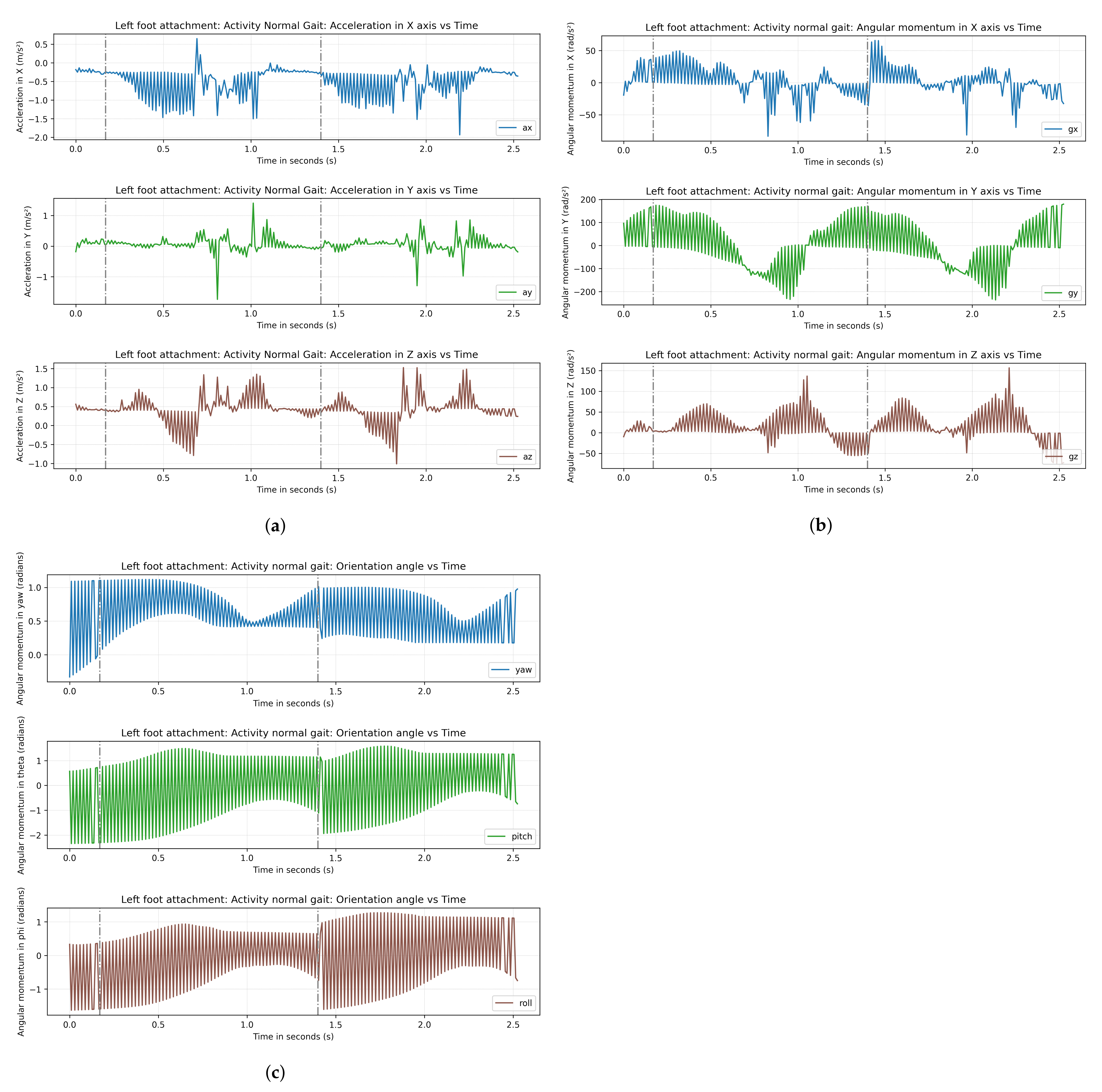
Figure 8 depicts the walking pattern of a healthy participant randomly chosen participant out of 21, which shows the characteristic signals of acceleration, gyroscope, and Euler angle components versus time. The figure shows that a gait pattern repeats after a certain interval, indicated by dotted lines in
Figure 8a–c. For this participant, the interval for the pattern repetition was approximately 1.2 s for the walking activity.
5.3. Best Models
The dataset underwent the model training procedure as described in
Section 3.4, followed by the model evaluation procedure as described in
Section 3.5. The best model was chosen from the output of the various overlapping datasets for each deep learning architecture. Almost all of the best models for all architectures were found at an 80% overlap of datasets. The training process description and testing results for all three architectures are discussed below:
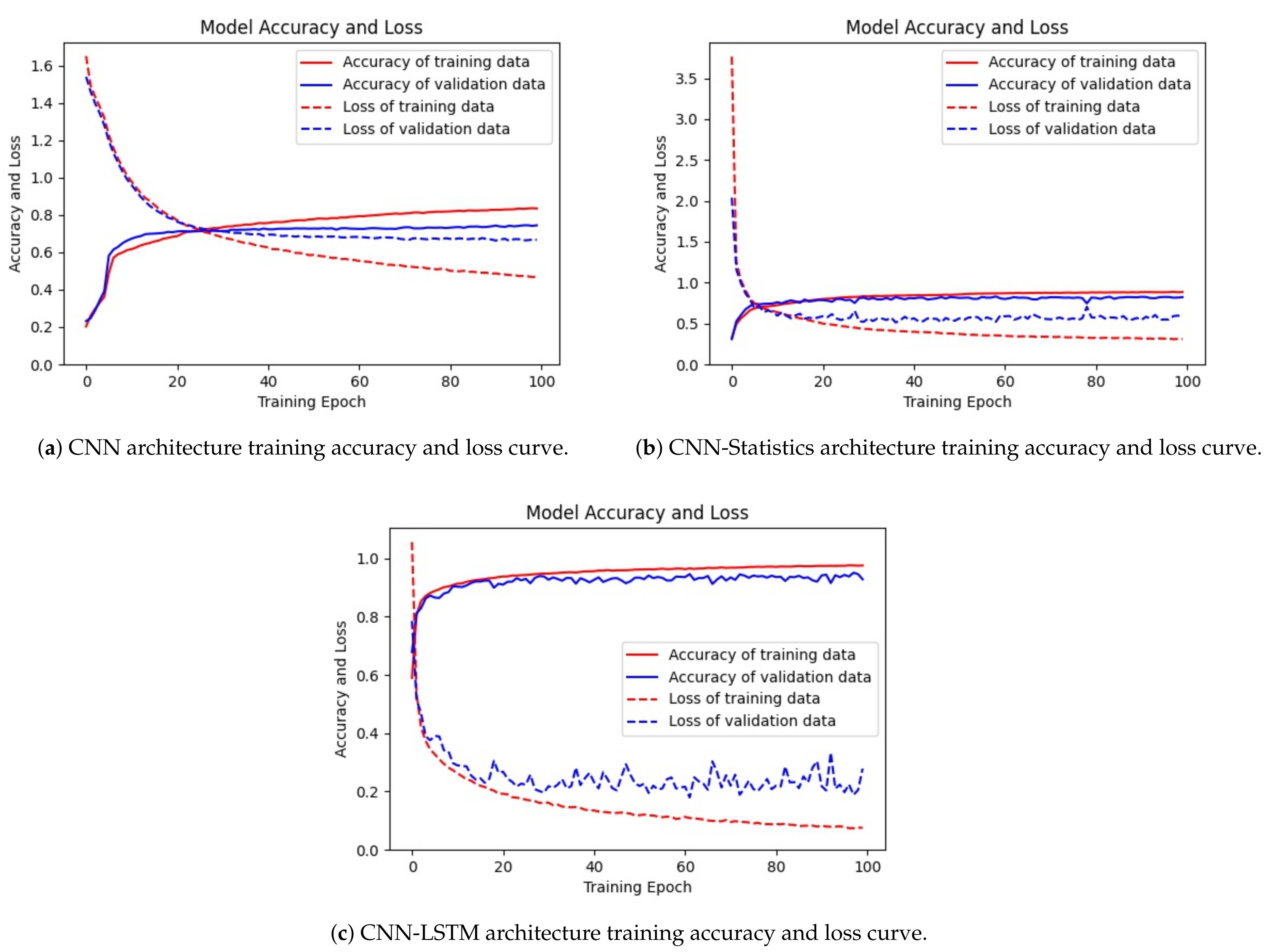
Firstly,
Figure 9a shows the results of the train/test loss and accuracy versus the total number of epochs for 80% overlap. The loss starts at approximately 1.6 and gradually decreases until the 40th epoch, while the training and validation accuracy increases sharply until the 10th epoch and gradually increases afterward until approximately 70%.
Secondly, a similar result was found using the CNN-Statistics model (80% overlap) in
Figure 9b. Using statistical features also helps the training procedure achieve faster convergence, as the loss decreases sharply at the beginning. The main difference with a simple CNN model is that the optimizer’s convergence at the beginning of the training procedure is relatively fast. The values of the training loss and testing loss are close to each other, and the accuracy of the training and test data is also close, indicating that no overfitting occurred during the training procedure.
Finally,
Figure 10c shows the training and testing results of the CNN-LSTM model from the 80% overlap dataset. The train/validation accuracy is similar to the train/validation losses. The maximum validation accuracy is approximately 95%, and the minimum validation loss is approximately 0.2. The best model was saved to infer the test data.
In conclusion, among the above CNN and CNN-Statistics architecture, the CNN-LSTM outperformed both models during the training and testing procedure. The validation accuracy achieved for this model was approximately 84%, while the test accuracy achieved for this model was approximately 88%.
5.4. Evaluation Metrics
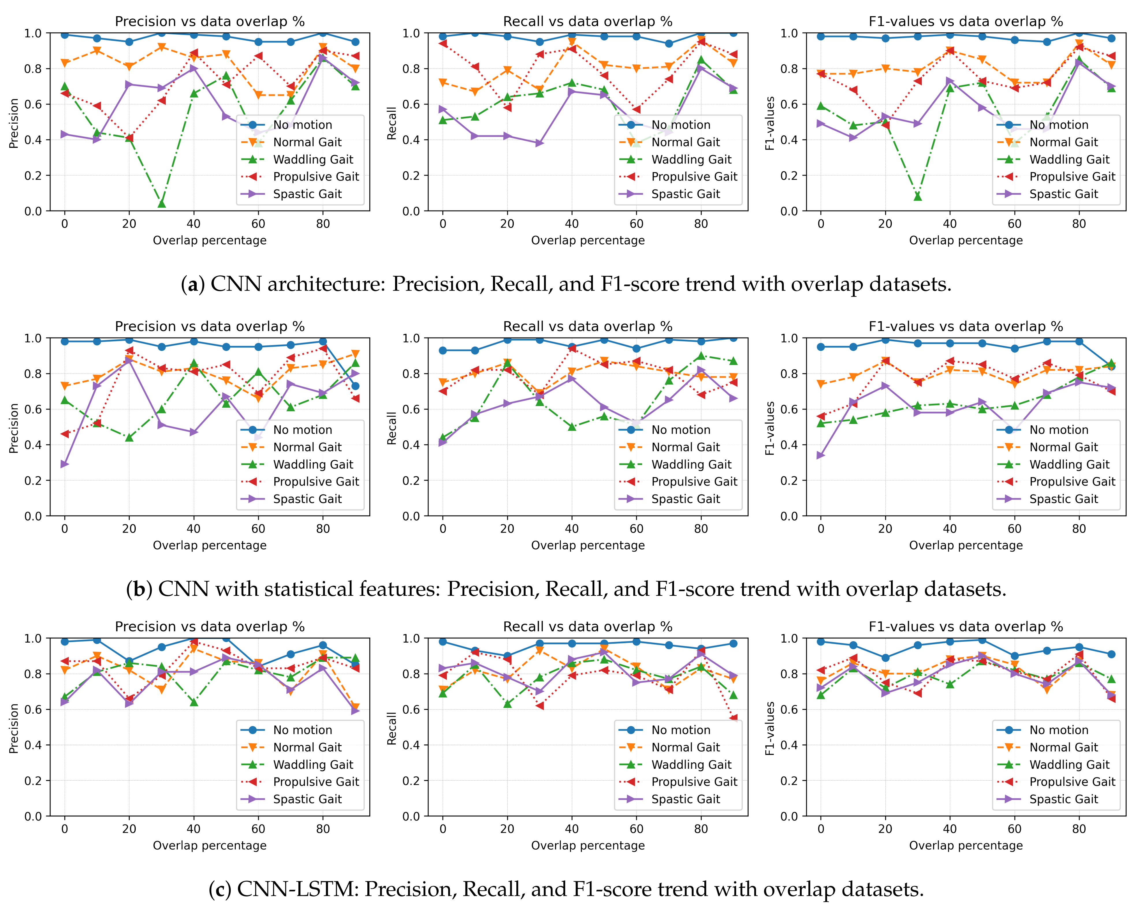
Figure 10a shows the recall, precision, and F1-score for all gait activities with overlapping datasets. The results indicate that for the no-activity class, all models across all overlapping datasets can generalize the class with approximately 100% precision, recall, and F1-score. For the other classes, precision, recall, and F1-score range from approximately 40% to 90%. Furthermore, the figure shows that the CNN model struggles to generalize to other gait classes, with the exception of the no-movement activity. However, there is an upward trend in precision, recall, and F1-score for all datasets as the overlap increases.
Figure 10b shows the precision, recall, and F1-score for the CNN-Statistics model for all gait activities for different overlapping datasets. A trend can be seen where precision, recall, and F1 values increase as the overlap increases for all gait activities. Comparatively, the CNN-Statistics model has better generalization than the CNN network, as seen in the training dataset of 80% overlap where the F1-score, recall, and precision values are all above 65%, while for the CNN model, they are just above 40%. The figure shows that precision, recall, and F1-score decrease for 90% overlap, indicating overfitting. However, until 80% overlap, the model has the highest precision, recall, and F1 values, indicating neither overfitting nor underfitting.
Figure 10c shows that the CNN-LSTM has higher generalization capability compared to the other architectures during the testing process. The precision, recall, and F1-score for all overlapping datasets are above 70%. The maximum precision, recall, and F1-score can be observed at 80% overlap, where for all captured gait activities, the percentage is above 80%.
5.5. Loss and Accuracy Evaluation
Table 6 shows the validation/training loss and validation/training accuracy for all model architectures, as well as the relationship between overlapping datasets and loss and accuracy metrics. For the CNN architecture, the maximum validation accuracy and minimum validation loss are achieved at 80% overlap. The test loss is at approximately 0.33 and the test accuracy is approximately 0.90. As overlap increases, there is a significant improvement in the test loss and test accuracy.
For the CNN-Stats architecture, the highest validation accuracy and lowest validation loss are achieved at 70% overlap. However, the minimum test loss and accuracy are achieved at 80% overlap, with values of 0.55 and 83%, respectively. At 80% overlap, the validation loss and test loss are similar, indicating that the model is neither underfitting nor overfitting. The best model for the CNN-LSTM architecture is found at 50% overlap, with the highest test accuracy and lowest loss of approximately 0.91 and 0.28, respectively.
Based on validation/test losses and validation/test accuracy, the best models for CNN, CNN-Stats, and CNN-LSTM are chosen with 80%, 80%, and 50% overlapping data, respectively.
5.6. Overlapping Dataset Accuracy and Loss Trend
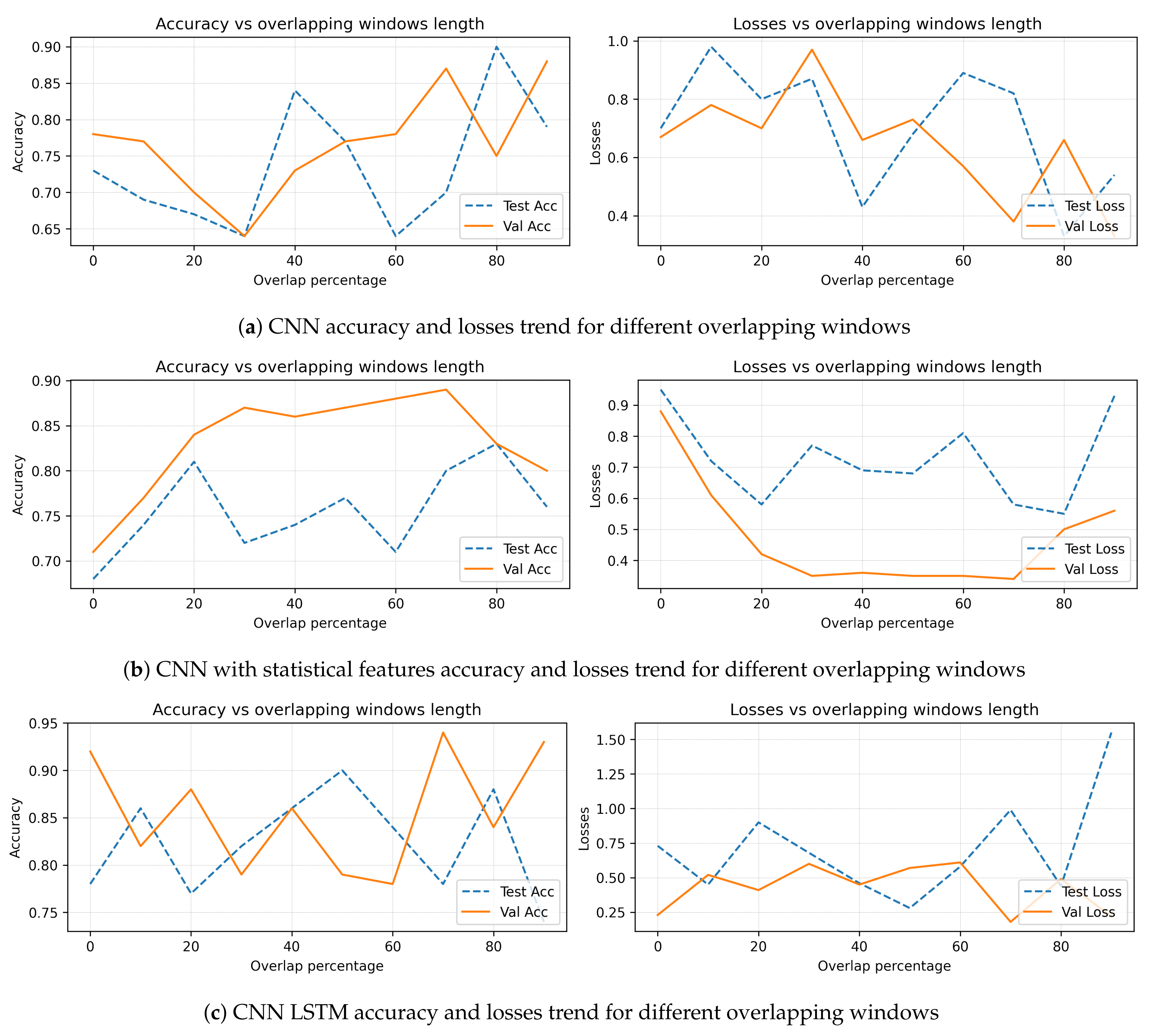
Increasing both the test and validation accuracy can be seen as the overlapping of data increases. Similarly, a trend of decreasing loss can be seen for both test and validation loss as the overlapping of data increases. For a simple CNN network, a significant impact on the test accuracy and loss can be seen in
Figure 11a.
In
Figure 11b, it can be seen that the validation and test accuracy increase as the percentage of overlapping data increases, and similarly, the validation and test loss decrease as the overlap percentage increases. However, accuracy decreases and loss increases at higher percentages of overlapping data, suggesting that the model tends to overfit a higher percentage of the overlapping dataset for the CNN statistical feature network. On the other hand, in
Figure 11c, the relationship between accuracy and loss for the CNN-LSTM architecture shows that the overlapping dataset does not significantly impact the accuracy or loss during training. The trend for all overlapping data is quite similar. However, the test loss is observed to be higher at higher percentages of overlapping datasets for this architecture.
5.7. Deployment Results
The final model was chosen based on the minimum test loss and maximum accuracy and was subject to post-training quantization.
Table 7 shows the size of the deep learning models in kilobytes (kB). The smallest model is the CNN model with approximately 224.5 kB, and the largest one is the CNN-LSTM with approximately 1700 kB.
The Keras model was converted to TensorFlow.js [
28] format to run the inferences on a Raspberry Pi 3. The data logger software was modified to include a feature for handling the inference. A circular buffer was implemented to store the accelerometer data for a length of 128. All of the converted TensorFlow.js models were deployed to the Raspberry Pi.
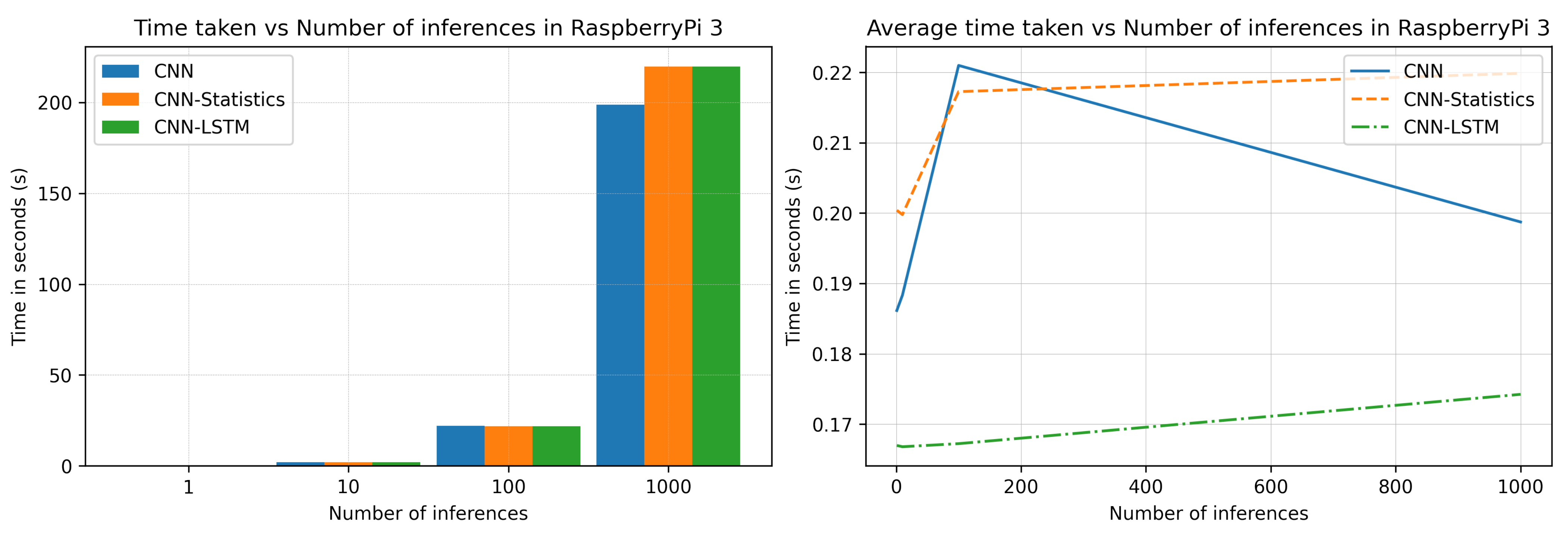
The benchmarks for the inference can be seen in
Figure 12, where the time taken for the CNN-LSTM model is much faster for 1000 inferences than for CNN models. The total and average inference times for both CNN and CNN statistic models are similar. In contrast, the average inference time for the CNN-LSTM model is faster than other models by approximately 300 milliseconds for 1000 inferences.
In summary, the test results for the CNN, CNN-Stats, and CNN-LSTM models were satisfactory, with accuracy levels above the 85% confidence level. The inference time for these models on a single CPU of 1.2 GHz Raspberry Pi 3 was less than 0.2 s. Among the models, the simple CNN network had the smallest memory footprint, while CNN-LSTM had the largest memory footprint. However, during the post-quantization conversion, the generalization capability of the models was not preserved, resulting in damage to the models. Consequently, the deployment of the models to the microcontroller was not entirely successful. However, an alternative method was used to deploy the models to the Raspberry Pi B+ model. The detailed summary is provided in
Table 8.
The results of the proposed study and other research are listed in
Table 9. Most of the research has not focused on deployment and inference on low-powered embedded devices. Our study fills the gap between model deployment and inference techniques in ARM SoC. In comparison with [
29], which employs a single IMU sensor attached to the participant’s waist, our study attaches the sensor to a single foot during the inference stage, opening up the possibility of targeting a wider audience with wearable foot sensors instead of belts. Additionally, our study provides proof of concept for the multi-label classification of pathological gait, whereas the previous study is limited to binary classification. Compared with other studies such as [
16,
29], our accuracy is slightly lower because the main focus of the study was model deployment and inference on memory-constrained devices. It would have been possible to achieve higher accuracy by taking more parameters into consideration, but this would have increased the model size. Therefore, we aimed to strike a balance between accuracy and memory size to make the model deployable without sacrificing too much accuracy during the inference process. This study was able to provide a bridge between the gap using the above methodology and results.


