
Performance Modeling and Optimization for a Fog-Based IoT Platform

Department of Electrical and Computer Engineering, St. Cloud State University, St. Cloud, MN 56301, USA
IoT 2023, 4(2), 183-201; https://doi.org/10.3390/iot4020010
Submission received: 29 April 2023
/
Revised: 26 May 2023
/
Accepted: 27 May 2023
/
Published: 2 June 2023
Abstract
:A fog-based IoT platform model involving three layers, i.e., IoT devices, fog nodes, and the cloud, was proposed using an open Jackson network with feedback. The system performance was analyzed for individual subsystems, and the overall system was based on different input parameters. Interesting performance metrics were derived from analytical results. A resource optimization problem was developed and solved to determine the optimal service rates at individual fog nodes under some constraint conditions. Numerical evaluations for the performance and the optimization problem are provided for further understanding of the analysis. The modeling and analysis, as well as the optimization design method, are expected to provide a useful reference for the design and evaluation of fog computing systems.
1. Introduction
The Internet of Things (IoT) describes the network of physical objects embedded with sensors, microcontrollers, software, and other technologies for the purpose of connecting and exchanging data with other devices and systems over the Internet [1,2]. A typical IoT platform works by continuously sending, receiving, and processing data in a feedback loop. IoT devices are the nonstandard computing devices such as smart TVs, smart sensors, smartphones, and smart security robots that connect wirelessly to a network and have the ability to transmit data. Fog devices are where the data are collected and processed.
Fog computing, also known as edge computing, is an architecture that uses fog nodes to receive tasks from IoT devices and perform a large amount of computation, storage, and communication locally, and may route processed data over the Internet to the cloud for further processing if necessary. The goal of fog computing is to improve the efficiency of local and cloud data storage. Fog computing can handle massive data initiated from IoT devices on the edge of networks. Because of its characteristics like low latency, mobility, and heterogeneity, fog computing is considered to be the best platform for IoT applications, sometimes called a fog-based IoT platform. For example, fog computing reduces the amount of data that needs to be sent to the cloud and keeps the latency to a minimum, which is a key requirement for time-sensitive applications such as IoT-based healthcare services [3]. Another example is, in a fog-based IoT platform for smart buildings, the information about the indoor ambience is collected in real-time by IoT devices and sent to the fog for aggregating and preprocessing before being passed to the cloud for storage and analysis. Proper decisions are made and sent back to the related actuators to set the ambience accordingly, or to fire an alarm [4]. More investigation about the essential components of fog-based architecture for IoT systems and their implementation approaches is surveyed in [5].
Fog and cloud concepts are very similar to each other, however, there are some differences. Here is a brief comparison of fog computing and cloud computing: (1) Cloud architecture is centralized and consists of large data centers located around the globe; fog architecture is distributed and consists of many small nodes located as close to client devices as possible. (2) Data processing in cloud computing is in remote data centers. Fog processing and storage are done on the edge of the network close to the source of information, which is crucial for real-time control. (3) Cloud is more powerful than fog regarding computing capabilities and storage capacity, but fog is more secure due to its distributed architecture. (4) Cloud performs long-term deep analysis due to slower responsiveness, while fog aims for short-term edge analysis due to instant responsiveness. (5) A cloud system collapses without an Internet connection. Fog computing has a much lower risk of failure due to using various protocols and standards. Overall, while both cloud and fog computing have their respective advantages, it is important to note that fog computing does not replace cloud computing but complements it. Choosing between these two systems depends largely on the specific needs and goals of the user or developer.
Fog computing is especially important in IoT deployment as it frees resource-constrained IoT devices from having to frequently access the resource-rich cloud [6]. Since the IoT tasks of requesting fog computing resources and service types are variable, dynamically provisioning fog computing resources to ensure optimum resource utilization and at the same time meet a certain constraint will not be an easy task. To optimize the fog computing resources and assure the required system performance, the system modeling and performance analysis for a fog-based IoT platform is an important development step for commercial IoT network deployment.
In this paper, we propose a fog-based IoT platform model involving three layers, i.e., IoT devices, fog nodes, and the cloud, using a queueing network with feedback and analyzing the performance of individual subsystems and the overall system based on different parameters such as the external arrival rates, fog node service rates, and routing probabilities. Some performance metrics of interest are derived such as the mean number of IoT tasks in the subsystems and the overall system, and the mean sojourn time in the subsystems and the overall system. Based on the queue length distribution at fog nodes, we solve a resource optimization problem that finds the optimal service rates at individual fog nodes under the constraint of a fixed total service capability of the fog computing system. Numerical evaluations are conducted for the derived performance metrics and the optimization problem.
The remainder of the paper is organized as follows. Section 2 illustrates various relevant works. Section 3 describes the fog-based IoT platform architecture. Section 4 uses queueing theory to investigate the performance modeling of individual subsystems and the overall system. Section 5 presents the resource optimization problem for the fog computing system. Section 6 presents the numerical evaluation. Finally, the paper is concluded in Section 7.
2. Related Work
The modelling, analysis and validation for fog computing systems, particularly with IoT applications, have been extensively studied in the literature. A brief summary of different research aspects is reviewed as follows. In [7], a set of new fall detection algorithms were investigated to facilitate fall detection process, and a real-time fall detection system employing fog computing paradigm was designed and employed to distribute the analytics throughout the network by splitting the detection task between the edge devices. In [8], a conceptual model of fog computing was presented, and its relation to cloud-based computing models for IoT was investigated. In [9], a new fog computing model was presented by inserting a management layer between the fog nodes and the cloud data center to manage and control resources and communication. This layer addresses the heterogeneity nature of fog computing and its challenging complex connectivity. Simulation results showed that the management layer achieves less bandwidth consumption and execution time. In [10], a health monitoring system with Electrocardiogram (ECG) feature extraction as the case study was proposed by exploiting the concept of fog computing at smart gateways providing advanced techniques and services. ECG signals are analyzed in smart gateways with features extracted including heart rate, P wave and T wave. The experimental results showed that fog computing helps achieve more than 90% bandwidth efficiency and offers low-latency real-time response at the edge of the network.
In [11], a charging mechanism called “FogSpot” was introduced to study the emerging market of provisioning low latency applications over the fog infrastructure. In FogSpot, cloudlets offer their resources in the form of Virtual Machines (VMs) via markets. FogSpot associates each cloudlet with a price that targets to maximize cloudlet’s resource utilization. In [12], a distributed dataflow (DDF) programming model was proposed for an IoT application in the fog. The model was evaluated by implementing a DDF framework based on an open-source flow-based run-time and visual programming tool called Node-RED, showing that the proposed approach eases the development process and is scalable. In [13], a complex event processing (CEP) based fog architecture was proposed for real-time IoT applications that use a publish-subscribe protocol. A testbed was developed to assess the effectiveness and cost of the proposal in terms of latency and resource usage. In [14], an alternative to the hierarchical approach was proposed using the self-organizing computer nodes. These nodes organize themselves into a flat model, which leverages on the network properties to provide improved performance.
In [15], a dynamic computation offloading framework was proposed for fog computing to determine how many tasks from IoT devices should be run on servers and how many should be run locally in a vibrant environment. The proposed algorithm makes dynamic decisions of offloading according to CPU usage, delay sensitivity, residual energy, task size and bandwidth, as well as by sending time-sensitive tasks to local devices or fog nodes for processing and resource-intensive tasks to the cloud. In [16], a distributed machine learning model was proposed to investigate the benefits of fog computing for industrial IoT. The proposed framework was implemented and tested in a real-world testbed for making quantitative measurements and evaluating the system. In [17], a resource-aware placement of a data analytics platform was studied in fog computing architecture, seeking to adaptively deploy the analytic platform, and thus reducing the network costs and response time for the user.
In [18], a joint optimization framework was proposed for computing resource allocations in three-tier IoT fog networks involving all fog nodes (FNs), data service operators (DSOs), and data service subscribers (DSSs). The proposed framework allocates the limited computing resources of FNs to all the DSSs to achieve an optimal and stable performance in a distributed fashion. In [19], a container migration mechanism was presented in fog computing that supports the performance and latency optimization through an autonomic architecture based on the MAPE-K control loop, providing a foundation for the analysis and optimization design for IoT applications. In [20], a market-based framework was proposed for a fog computing network that enables the cloud layer and the fog layer to allocate resources in the form of pricing, payment, and supply–demand relationship. Utility optimization models were investigated to achieve optimal payment and optimal resource allocation via convex optimization techniques, and a gradient-based iterative algorithm was proposed to optimize the utilities.
Although fog computing is considered to be the best platform for IoT applications, it has some major issues in the authentication, privacy, and security aspects. Authentication is one of the most concerning issues of fog computing, since fog services are offered at a large scale. This complicates the whole structure and trust situation of fog. A rouge fog node may pretend to be legal and coax the end user to connect to it. Once a user connects to it, it can manipulate the signals coming to and from the user to the cloud and can easily launch attacks. Since fog computing is mainly based on wireless technology, the issue of network privacy has attracted much attention. There are so many fog nodes that every end user can access them, thus more sensitive information is passed from end users to fog nodes. Fog computing security concerns arise as there are many IoT devices connected to fog nodes. Every device has a different IP address, and any hacker can forge your IP address to gain access to your personal information stored in the particular fog node. In [21], a lightweight anonymous authentication and secure communication scheme was proposed for fog computing services, which uses one-way hash function and bitwise XOR operations for authentication among cloud and fog, with a user and a session key agreed upon by both fog-based participants to encrypt the subsequent communication messages. More references can be found in [22,23] that survey main security and privacy challenges of fog and edge computing, and the effect of these security issues on the implementation of fog computing.
3. A Fog-Based IoT Platform Architecture
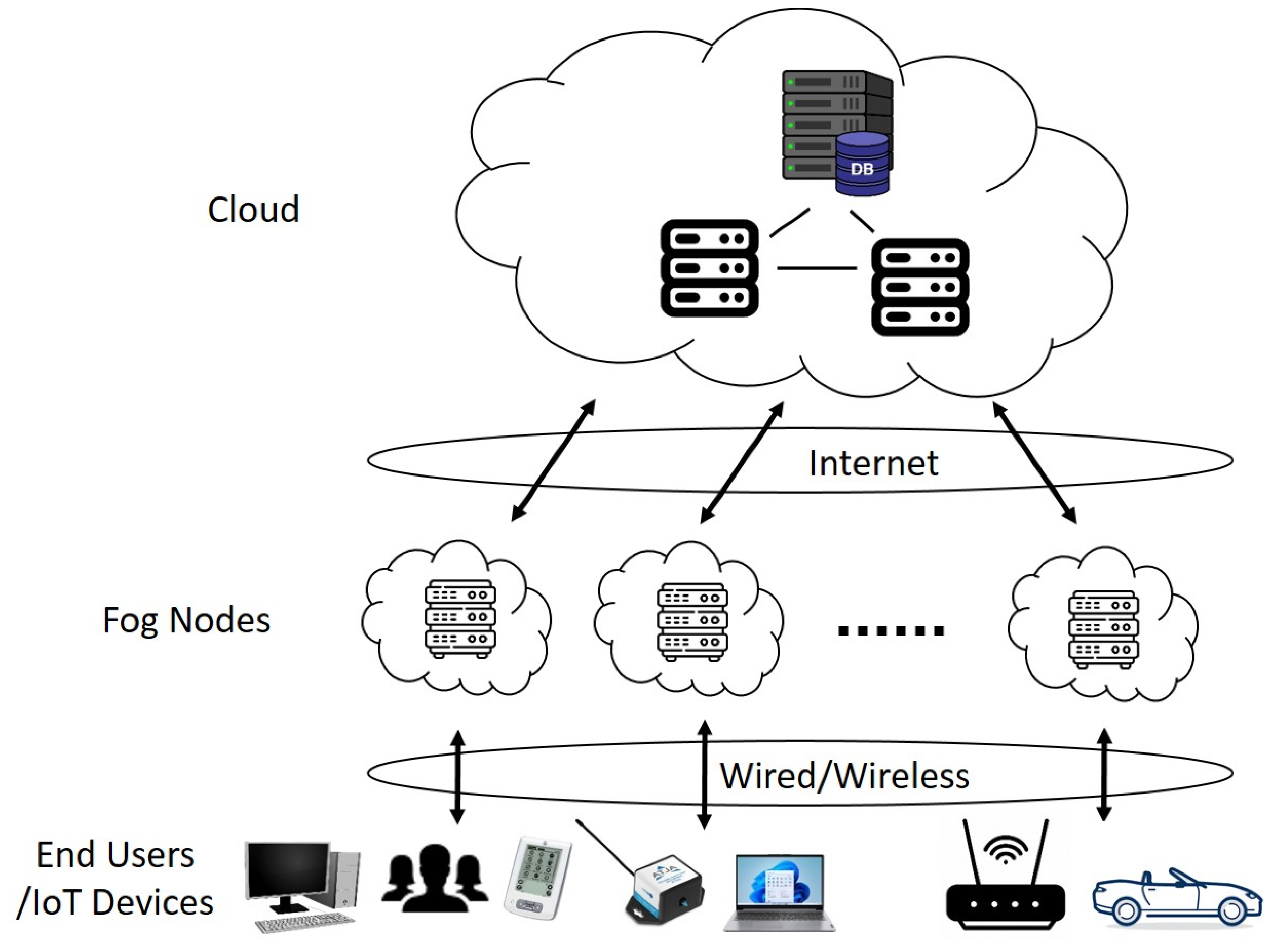
Fog computing is a decentralized computing infrastructure in which data, computer storage and applications are located somewhere between the source (end user) and the cloud. Thus, fog computing brings the advantages and power of the cloud closer to end users. The proposed fog computing architecture (i.e., the fog-based IoT platform) comprises three layers: IoT devices, fog nodes, and cloud, as shown in Figure 1. The need for smart control and decision-making at each layer depends on the time sensitivity of an IoT application.
The lowest layer is the end user layer, which consists of a large number of IoT devices, such as robots, smart security, smart phones, wearable devices, smart watches, smart glasses, laptops, and autonomous vehicles. Some of these devices may have the capability of computing, while others may only collect raw data through intelligent sensing of objects or events and send the collected data to the upper layer for processing and storage.
The middle layer is the fog layer consisting of a group of fog nodes, such as routers, gateways, switchers, access points, base stations, and fog servers. Fog nodes are independent devices that calculate, transmit, and temporarily store the generated data from IoT devices, while a fog server also computes the data to make decision of an action. Other fog devices are usually linked to fog servers. Fog nodes can be deployed in a fixed position or on a moving vehicle and are linked to IoT devices to provide intelligent services. Fog nodes are located closer to the IoT devices compared with the cloud and, thus, in this way allow real-time analysis and delay-sensitive applications to be performed within the fog layer. Fog nodes are usually involved when an IoT device does not have data processing capability, or the generated data amount is too large for an IoT device (with computing capability) to process locally. Fog nodes are also connected to the upper layer cloud data centers through the Internet, and can obtain more powerful computing and storage capabilities for some large and complex data processing tasks.
The upper layer is the cloud layer, which includes many servers and storage devices with powerful computing and storage capabilities to provide intelligent application services. This layer can support a wide range of computational analysis and storage of large amounts of data. However, unlike the traditional cloud computing architecture, fog computing does not handle all computing and storage through the cloud. Fog nodes themselves have appropriate computing and storage capabilities. According to the data processing load and quality of service (QoS) requirements, some control strategies can be used to effectively manage and schedule the processing tasks between fog nodes and the cloud, to improve the utilization rate of the overall system resources.
The data transmission between the end users and the fog nodes may be in wired or wireless modes. The selection of the connectivity mode depends mostly on an IoT application. One may think that wired connectivity is generally faster and more secure than the wireless mode. The major wireless technologies for the IoT communication protocols include Bluetooth low energy (BLE) [24], Zigbee [25], Z-Wave [26], WiFi [27], cellular (GSM, 4G LTE, 5G), NFC [28], and LoRaWAN [29]. These IoT communication protocols cater to and fulfill the specific functional requirements of IoT systems. The Internet connection acts as the bridge between the fog layer and the cloud layer and establishes the interaction and communication between them.
4. Performance Modeling and Analysis
From the previous system description, we built the performance model by using an open queueing network with feedback for the proposed fog computing system. A fog computing system can offer and deliver services through a group of fog nodes offered by a service provider. The end users (IoT devices) can send tasks to the fog nodes to access the offered services. Each fog node can be considered as a single server. After an IoT device receives its service at the fog node, it may enter an exit server and leave the system if no further service is needed, or it continues to receive service in a cloud server if the fog node cannot provide further service to it.
The cloud has huge types of resources connected through the Internet, and multiple servers or virtual machines (VMs) can be used to support service requests. The servers or VMs can co-operate to offer services and may be considered as a huge virtual server that has enough support and processing capability, as our focus here is on fog computing service and thus all the cloud services are simplified as a whole, via a virtual server for tractable analysis. Every service request can get an immediate response when it is sent to the virtual server. After the cloud service is completed, the IoT task may enter an exit server and leave the system or go back to a fog node to continue receiving service.
The exit server performs administration and finance (A&F) management for all the IoT tasks that receive fog and/or cloud services, which is referred to as an A&F server. There may be multiple such exit servers distributed in different places in the cloud. They are interconnected through the Internet and share information with each other. Hence, similar to the treatment of the cloud, the exit servers are also considered as a huge virtual server that has sufficient support capability, which enables every IoT task to get an immediate service before leaving the system.
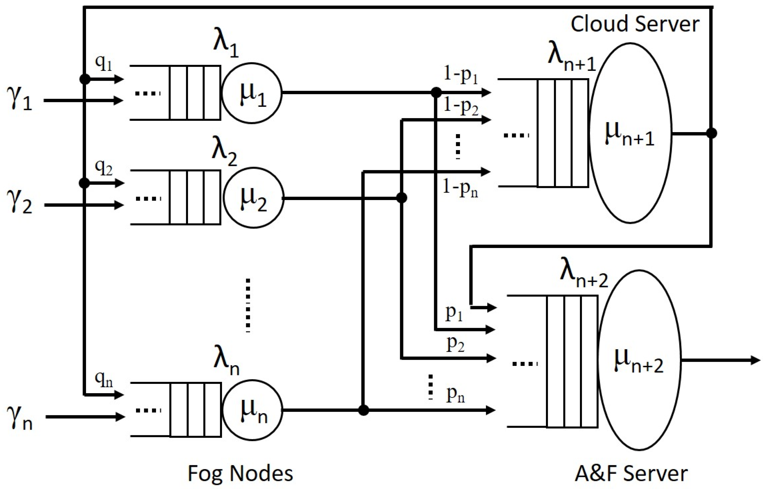
From the above analysis, we assume that there is a total of n fog nodes in the proposed fog computing system. Each fog node can be modeled as an M/M/1 queue with infinite queue (buffer). The cloud service server and the exit server are modeled as M/M/∞ queues, respectively [30]. The service discipline is first come first served (FCFS). Finally, the overall computing system forms an open queueing network with feedback, as shown in Figure 2.
Let the external arrivals of IoT tasks (service requests) to the ith fog node be a Poisson process with rate and service time be exponentially distributed with mean 1/μi, 1 ≤ i ≤ n. Upon the completion of a service at the ith fog node, the IoT task may enter the A&F server with probability pi for some administration and finance processing and then leave the system; the IoT task may also be routed to the cloud with probability 1 − pi to receive further service or processing at the cloud, based on demand. For example, a fog node may not be able to completely process an IoT task’s service request, then the service request will be sent to the cloud for further processing, as the cloud has much more powerful computing and storage capabilities compared with fog nodes. Upon the completion of the service at the cloud, the IoT task may be fed back to the ith fog node with probability qi (1 ≤ i ≤ n) to continue receiving service, or directly enter the A&F server for exit processing with probability and then leave the system.
To summarize, the overall computing system is an open queueing network with n + 2 nodes, i.e., n fog nodes, 1 virtual cloud server and 1 A&F server. Node i consists of an infinite FCFS queue and an exponential server with different processing capability μi, 1 ≤ i ≤ n + 2. External task arrivals to node i form Poisson with rate . After the completion of service at node i, the task may proceed to node j with a probability independent of history or leave the system with another probability. Therefore, the system is a Jackson network [30].
Let λi denote the total average arrival rate of the IoT tasks to fog node i. This total rate is given by the sum of the external arrivals (Poisson) and the arrivals from all internal nodes (not necessarily Poisson). Thus, we obtain the following traffic equations:
The above first n + 1 traffic equations can be expressed in vector form as follows:
where , , and the routing probability matrix R (note that here R is not a traditional transition probability matrix in a queueing system) is
Since the matrix is invertible, Equation (5) has a unique solution given by
4.1. Modeling of the Fog Layer Subsystem
The fog layer can be modeled by n infinite single server queues with Poisson arrivals and exponentially distributed service times. Since IoT devices are limited in terms of communication capabilities, processing power, and energy consumption due to their low cost, they are very heterogeneous in terms of their processing requirements, device data formats, communication protocols, and transmission technologies. Thus, these M/M/1 queues are modeled with different effective arrival rates λi and different service rates μi at individual fog nodes. Assume that the service time in node i is independent from that in other nodes and is also independent of the arrival process. Using the traditional method of flow balance equations [30], we solve the steady state probabilities with k service requests in node i as:
where is the traffic intensity, or utilization factor, at node i, , and is the probability of an empty queue and is determined by the normalization condition () as:
The probability that node i contains at least m service requests, denoted by , can be determined as:
The mean number of service requests in node I, denoted by , can be calculated as:
The mean number of service requests waiting in the queue of node i, denoted by , is thus determined as:
The mean number of service requests (including the requests in the server and in the queue of fog nodes) in the fog subsystem which includes n nodes, denoted by , can be calculated as:
The mean sojourn time in node i, i.e., the response time from the moment a service request arrives at node i to the moment it leaves node i, denoted by , can be obtained by Little’s law:
The mean waiting time on a visit to node i, denoted by , is:
4.2. Modeling of the Cloud and the A&F Server
As mentioned previously, we simplify the cloud service and the A&F service respectively as a huge virtual server and model them as M/M/∞ queues, which means that they have large enough support and processing capability for all IoT service requests (equivalent to an infinite number of servers). We apply the method of balance equations [30] to determine the probabilities, denoted by for the cloud server and for the A&F server, that the server contains k service requests as:
By normalization condition, the probability is determined as:
Since no customer waits in an M/M/∞ queue, the mean sojourn time in the server must be equal to the mean service time 1/μi, i = n + 1, n + 2, and the mean number of customers in the server can be obtained by Little’s law:
The mean sojourn time in the server, denoted by , can be calculated by Little’s law:
By combining Equations (2) and (3), we can represent in term of the external arrival rates, , as:
which verifies the fact that at equilibrium, the total rate at which service requests arrive into a queueing network from the outside must be equal to the rate at which they leave the network.
4.3. Modeling of the Overall IoT Platform System
By combining all three layers of architecture, we obtain a simple version of an open Jackson network with (n + 2) nodes, where the first n nodes are the M/M/1 queues describing the fog nodes with external arrival rate and service rate , 1 ≤ i ≤ n. Node n + 1 and node n + 2 are the M/M/∞ queues with the arrival rate of λi and service rate of μi at each server, i = n + 1, n + 2.
By Jackson’s theorem [31], the steady state probability distribution of the overall system state (k0, k1, …, kn) exhibits the product-form solution and is given by the product of the steady state distributions of individual queues, i.e.,
where refers to in (7) and (15), respectively. Note that the system stability condition must be satisfied, i.e., , 1 ≤ i ≤ n + 2.
Some performance metrics of the overall computing system can be determined as follows.
The mean throughput of the overall system, denoted by , is equal to the total external arrival rate to the system, i.e.:
The mean number of service requests in the overall computing system, denoted by L, is the sum of the number of requests () in all the n + 2 nodes at steady state.
The mean sojourn time in the overall computing system, i.e., the mean total response time from the moment a service request arrives at the system to the moment it leaves the system, denoted by T, can be calculated by Little’s law:
Note that , as is the mean time that a service request spends at node i during each visit at that node and a request may visit a node multiple times. From Equations (13) and (18), can be summarized as:
The mean number of visits that a service request to node i, also known as the visit ratio [32] at node i, is determined as:
Applying Equations (19) and (21), we have , which is consistent to the fact of the proposed system, i.e., every service request leaves the system only one time from the A&F server.
Finally, we simply discuss the computational complexity of the overall computing system. The computational complexity is mainly due to computing the matrix inverse in Equation (6), as the system metrics such as L, T and must use {} for computation. The maximum complexity for computing an matrix inverse will be if the Gaussian elimination method is used [33]; while the computational cost of the rest parts in L or T is only , which is ignored, and the final computational complexity is thus . For the present microprocessor capabilities and fog computing requirements, this small computational complexity is not an issue at all. It is worthy to note that the number of fog nodes n is variable, thus the proposed model is scalable and has the ability to increase or decrease its computing and storage resources as needed to meet various levels of demand.
5. Optimization Problem
In practice, both service providers and end users are concerned about the mean sojourn time of a service request spent in the overall computing system. We re-write Equation (23) in terms of arrival rates and service rates as follows:
From the Jackson theorem [31], the queue length distribution at node i is independent of the state of other nodes. Each node in the fog layer is modeled as an M/M/1 queue, and the cloud and the A&F server are modeled as M/M/∞ queues. Suppose the service provider has control over the fog node service rates , , but with a budgetary constraint that fixes the total service capability to some constraint value , i.e., . Thus, aimed at minimizing the mean sojourn time T that a service request spends in the overall computing system, we construct the following convex optimization problem for the fog layer under a given set of external arrival rates {}:
where the total mean sojourn time T is determined by the mean time of all IoT service requests that is spent in the overall computing system. The fog layer consists of n fog node servers with service request arrival rate and service processing capability , . Clearly, the fog nodes are heterogeneous as all the values may be different. The other part of T is determined by the virtual cloud server and the A&F server, which will not be involved in the optimization process below as we focus on the optimization of the processing capabilities of the fog nodes. The total service capability of the fog nodes is fixed to some constraint value .
To solve this optimization question, we apply the method of Lagrange multipliers by defining the Lagrangian function, , as follows [34]:
where the new variable is referred to as the Lagrange multiplier. Due to the independence assumption in the fog layer, it is possible to separately optimize the individual service rates in different nodes. The optimal solutions can be obtained by nullifying the partial derivatives:
After some mathematical manipulations, we obtain:
Substituting into the constraint Equation (27), we have:
By combining the Equations (30) and (31) and applying some mathematical manipulations, the optimal solution can be determined as:
where the optimal solution of service capability in node i can be interpreted as two parts of service requirements: the first part aims at satisfying the effective arrival rate to the node; the second part aims at satisfying the extra service margin due to the constraint of the total service capability of the fog layer and the affection from other nodes.
6. Numerical Evaluation
In this section, we present numerical results for the three-layer IoT platform system by studying selected metrics with respect to (w.r.t.) various parameters. The typical parameter settings are given in Table 1 (All the γi values are set to be equal unless otherwise specified in individual figures; all the μi values are set to be equal unless otherwise specified in individual figures; all the pi and qi values are respectively set to be equal unless otherwise specified). Other values of related parameters are set separately in the figures to study the performance of the relevant metrics. Note that the time is represented in terms of a dimensionless time unit, which can be mapped to a specific unit of time.
The specific notation and configuration are defined as follows for numerical evaluation. The external arrival rate vector is , where all elements are set to be identical and each changes from 1 to 10 for numerical evaluation, and the total external arrival rate is ; the fog node service rate vector is , and the initial setting for numerical evaluation is , the cloud server and A&F server have the following service rates for numerical evaluation ; the routing probability vector entering the A&F server is , where all elements are set to be identical with initial value 0.5 for numerical evaluation, i.e., ; the routing probability vector entering back to the fog layer is , where all elements are set to be identical with initial value 0.05 for numerical evaluation, i.e., .
Figure 3 shows the mean number of service requests in the fog layer subsystem LFog with respect to different parameters. We observe that LFog will increase with the increase of the total external arrival rate γ or the decrease of the service rates (contained in the vector μvec). It is obvious that the increase in the external arrival rate will lead to the increase of the queueing length. Equivalently, the increase of the service processing time (or the decrease of the service rates) will cause more service requests to wait in the queue and thus lead to an increase of queueing length. We also observe that LFog will decrease with the increase of the number of fog nodes n given the fixed total external arrival rate γ. This is because more fog nodes participate in the service and reduce the service burden of each node.
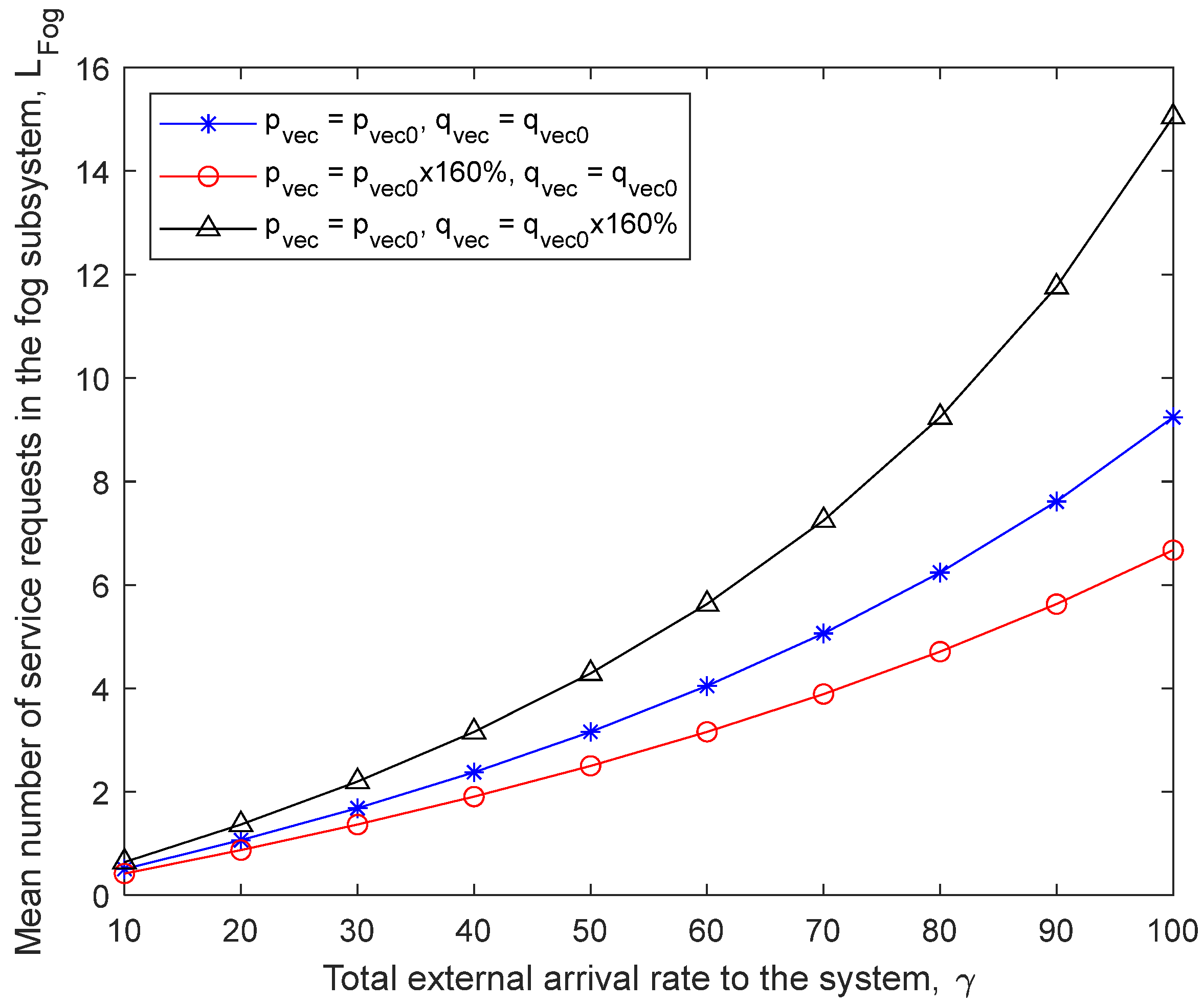
Figure 4 shows the mean number of service requests in the fog layer subsystem LFog with respect to different routing probabilities. We observe that, given the fixed fog node service rates μvec and the number of nodes n, LFog will decrease with the increase of the routing probabilities pvec or the increase with the increase of the routing probabilities qvec. When pvec increases, more service requests will enter the A&F server and then leave the system (instead of entering the cloud for further service), leading to a smaller number of requests in the system. On the contrary, when qvec increases, more service requests will be fed back to the fog layer subsystem for continuous service, leading to a larger number of requests in the system.
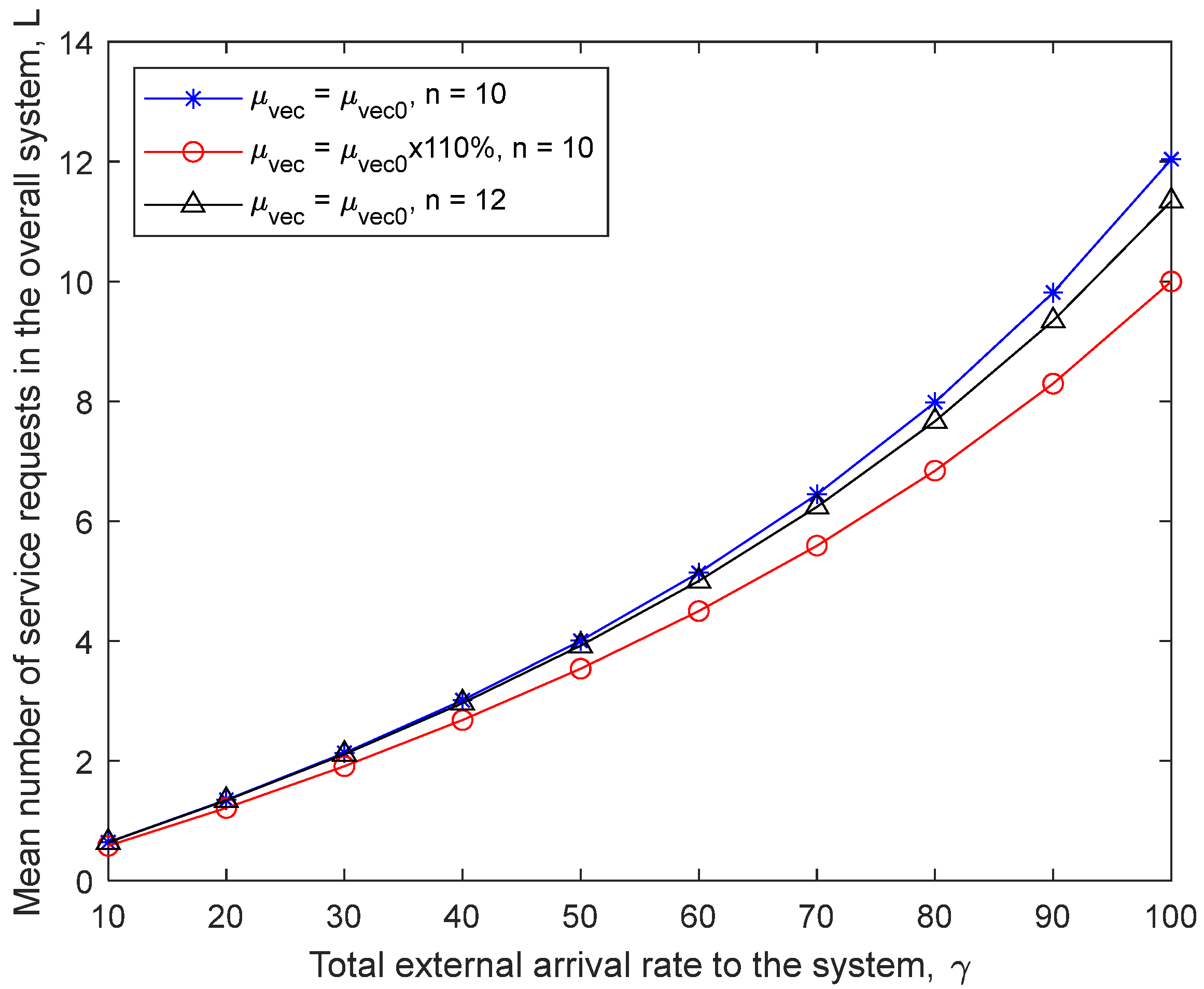
Similar to Figure 3 and Figure 4, Figure 5 and Figure 6 show the mean number of service requests in the overall computing system L with respect to different parameters. In Figure 5, we observe that L will decrease with the increase of the service rate vector μvec or increase of the number of fog nodes given the fixed total external arrival rate γ. In Figure 6, we observe that LFog will decrease with the increase of the routing probabilities pvec or increase with the increase of the routing probabilities qvec. The reason is the same as that explained previously.
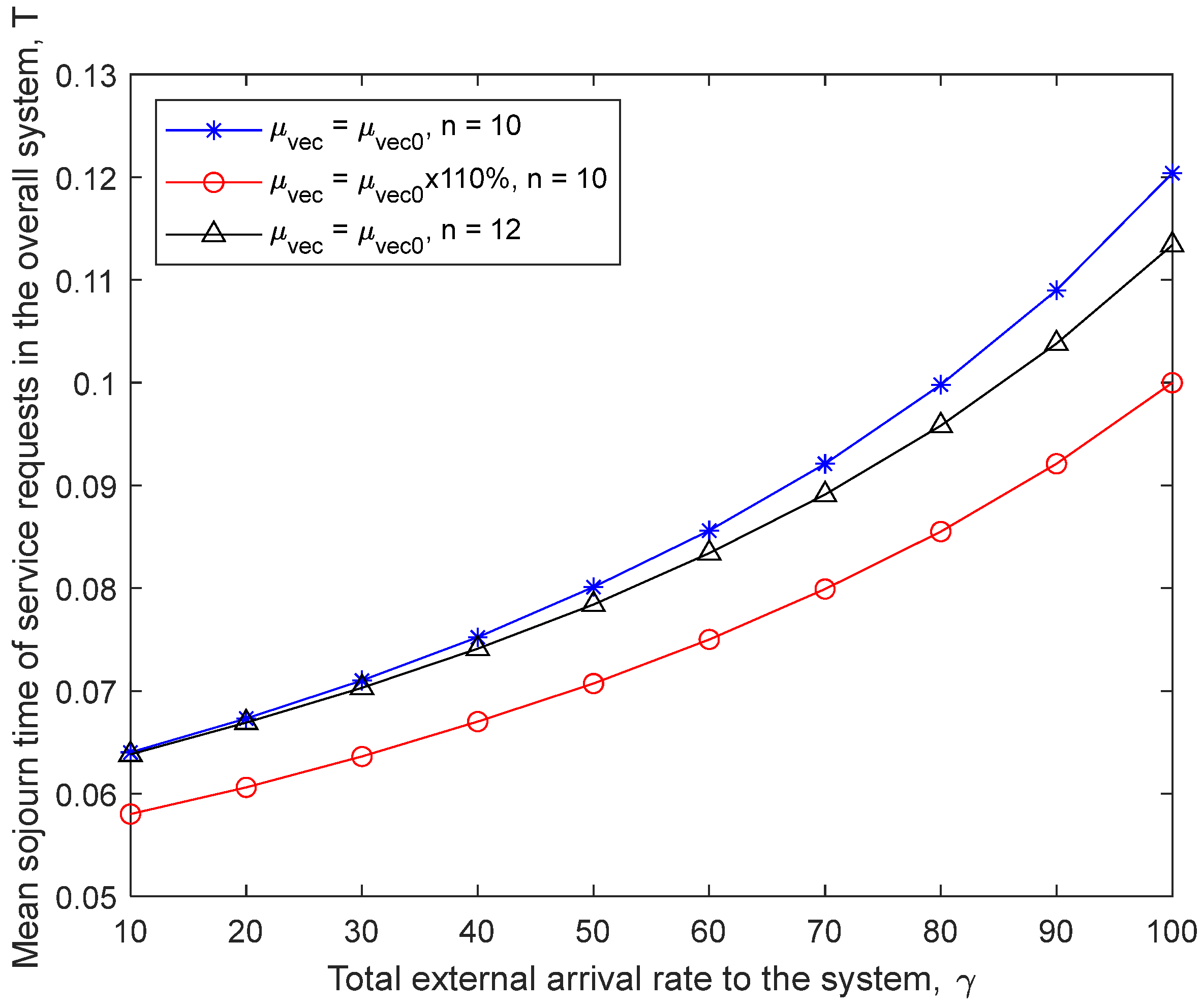
Figure 7 shows the mean sojourn time of service requests T with respect to the change of different parameters. As expected, T will increase with the increase of the arrival rate γ; T will decrease with the increase of the service rate vector μvec (e.g., μvec changes from μvec0 to 1.1 × μvec0) or with the increase of the number of fog nodes n (e.g., n changes from 10 to 12). The larger the arrival rate γ, the more the service requests waiting in the queue, which leads to a larger mean sojourn time of the requests in the system. Similarly, the larger the processing capability of the fog node servers, the fewer requests waiting in the queue, leading to less mean sojourn time. This is because more fog nodes make the mean waiting time less than expected.
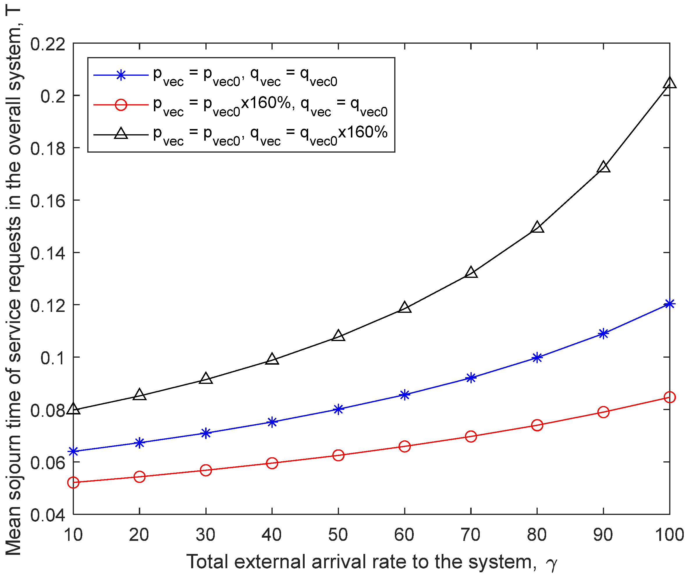
Figure 8 shows the mean sojourn time of service requests T with respect to different routing probabilities. We observe when pvec increases, e.g., from pvec0 to 1.6 × pvec0, T will be reduced quickly, particularly under the heavy traffic conditions. This can be explained as follows: the increase of the routing probabilities pvec means that more requests do not enter the cloud upon the completion of their service from the fog layer, which naturally reduces the mean waiting time and thus the mean sojourn time. We also observe that T will be increased with the increase of routing probabilities qvec, particularly under heavy traffic conditions. The increase of qvec means that more requests that have received service in the cloud will be fed back to the fog layer, which naturally causes more required mean waiting time of the requests and thus increases the mean sojourn time.
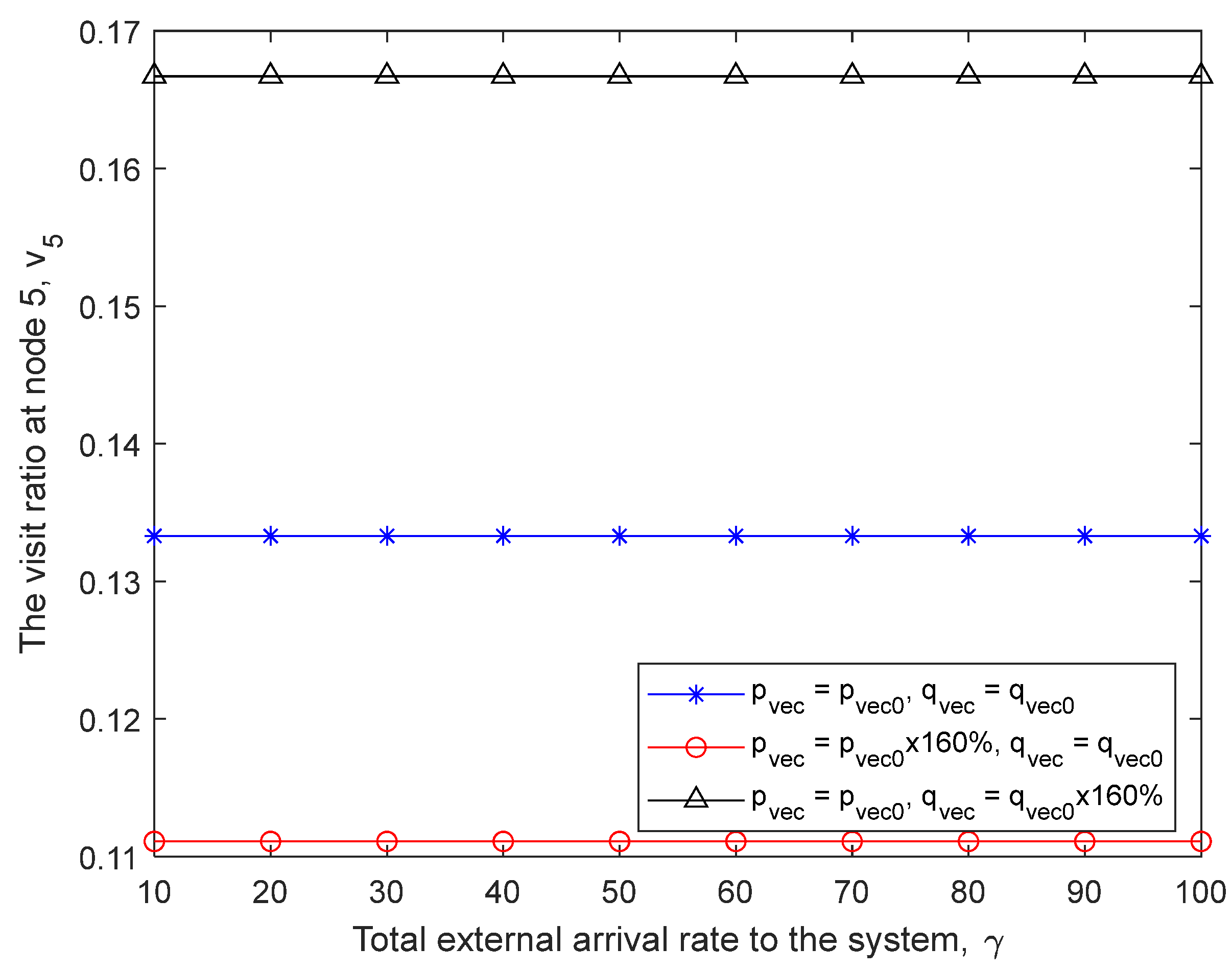
Figure 9 shows the visit ratio at a fog node v5 with respect to different routing probabilities. We use node 5 as an example for evaluation. We point out that any fog node produces the same result for the given input configuration, because we assume that all individual external arrival rates are set to be identical, which means that the individual effective arrival rates , , will be the same according to Equation (6). The above assumption and the obtained identical effective arrival rates will cause the visit ratio v5 not to change with different values of the total external arrival rate γ. This has been verified in Figure 9, where the visit ratio v5 is observed to be the same when γ is changed. We observe that v5 will be decreased when pvec increases, e.g., from pvec0 to 1.6 × pvec0. This is because the increase of the routing probabilities pvec causes more requests to enter the A&F server and exit the system upon the completion of their service from the fog layer, which naturally reduces the opportunity that a service request goes back to visit a fog node. We also observe that v5 will be increased with the increase of the probabilities qvec. The increase of qvec causes more requests that have received service in the cloud to go back to the fog layer, and thus increases the opportunity that a service request visits a fog node.
Next, we validate the optimization problem through numerical computation. To show the heterogeneous characteristics of IoT traffic, we assume that the traffic arrival rates from IoT devices to individual fog nodes are different, e.g., the initial setting of the external arrival rates to the n fog nodes is . The constraint value to the total service capability is set as C = 250 or 200 in different cases. The routing probabilities pvec and qvec are kept the same as before.
Table 2 shows the optimal solution of fog node service rates under the configuration set (, 250, , ), which is calculated by the analytical results in Section 5 and used as a benchmark for study. The optimal solution is copied from Table 2 as follows:
which has a similar trend to the given external arrival rate . For example, for the smallest external arrival rate , the assigned optimal service rate is also the smallest one, ; for the maximum rate , the assigned optimal service rate is also the maximum one, . This is consistent with the optimal resource allocation principle. Note that the sum of all elements in the optimal solution is 250, satisfying the constraint condition . The minimized mean sojourn time is T = 0.1336 time units.
Now we study the optimal solution under the condition when some parameter is changed. Table 3 shows the case when every external arrival rate is increased by 50% while other parameters do not change. We observe that the optimal solution in Table 3 has a similar property to Table 2. It is interesting to notice that although the external arrival rates are all increased by the same percentage, the optimal solution for some nodes are increased a little (e.g., ) but other nodes are decreased a little (e.g., ). It seems that there is no fixed rule to follow. This might be because the determination of the optimal solution is based on a global optimization principle. The minimized mean sojourn time for this case is T = 0.3989 time units. This is because the external arrival rates have increased as compared with Table 2.
If we change the total service capability of the fog layer C from 250 to 200, the optimal solution of the fog node service rates is determined in Table 4. As expected, the optimal solution of individual service rates tends to become smaller (with the constraint of C = 200). Similar to Table 2, we notice the smallest rate of and the maximum rate of due to the same reason. The minimized mean sojourn time for this case is T = 0.2455 time units, which is greater than 0.1336 time units due to the decrease of constraint value C.
On the basis of input data in Table 4, we increase the routing probabilities and , and study the optimal service rates. The results are presented in Table 5 and Table 6, respectively. Compared with Table 4, we observe that in Table 5 the optimal service rates change up and down slightly, but there are no definite rules to follow. Some service rates increase a little and some decrease a little. The overall change is minimal due to the fixed constraint of C. However, the minimized mean sojourn time becomes smaller: T = 0.1442 time units. This is because more service requests directly enter the A&F server and leave the system (instead of staying in the system to receive further service). Table 6 has a similar result to Table 5 except that the minimized mean sojourn time becomes larger: T = 0.8403 time units. This is because more service requests are fed back to the fog layer to continue receiving service after they complete their service in the cloud.
7. Conclusions
We developed a fog-based IoT platform model involving three layers, i.e., IoT devices, fog nodes, and the cloud using an open Jackson network with feedback, and we analyzed the performance of individual subsystems and the overall system based on different parameters such as the external arrival rates, fog node service rates, and routing probabilities. Interesting performance metrics were derived such as the mean number of service requests of the IoT devices to the fog subsystem and the overall system, and the mean sojourn time of service requests in the overall system. A resource optimization problem was developed and solved to determine the optimal service rates at individual fog nodes under the constraint of a fixed total service capability of the fog computing system. Numerical evaluations for the performance and the optimization problem were provided with detailed explanation for further understanding of the analysis. Note that in order to highlight the modeling and analysis of the fog layer characteristics, we have simplified all the cloud services as a huge virtual server with an M/M/∞ queue. Some interesting issues arising from this work will be further explored in our future research such as modeling of the cloud layer with a more specific queueing network based on cloud service types, modeling of nodes with buffers of finite capacity, and investigation of power saving strategies for the proposed model. The modeling and analysis, as well as the optimization design method, is expected to provide a useful reference for the design and evaluation of fog computing systems.
Funding
This research received no external funding.
Data Availability Statement
Not applicable.
Conflicts of Interest
The authors declare no conflict of interest.
References
- Sun, Y.; Song, H.; Jara, A.J.; Bie, R. Internet of Things and Big Data Analytics for Smart and Connected Communities. IEEE Access 2016, 4, 766–773. [Google Scholar] [CrossRef]
- Shafiq, M.; Gu, Z.; Cheikhrouhou, O.; Alhakami, W.; Hamam, H. The Rise of “Internet of Things”: Review and Open Research Issues Related to Detection and Prevention of IoT-Based Security Attacks. Wirel. Commun. Mob. Comput. 2022, 2022, 8669348. [Google Scholar] [CrossRef]
- Bonomi, F.; Milito, R.; Zhu, J.; Addepalli, S. Fog computing and its role in the internet of things. In Proceedings of the First Edition of the MCC Workshop on Mobile Cloud Computing, Helsinki, Finland, 17 August 2012; pp. 13–16. [Google Scholar] [CrossRef]
- Alsuhli, G.; Khattab, A. A Fog-based IoT Platform for Smart Buildings. In Proceedings of the 2019 International Conference on Innovative Trends in Computer Engineering (ITCE), Aswan, Egypt, 2–4 February 2019; pp. 174–179. [Google Scholar] [CrossRef]
- Sadatacharapandi, T.P.; Padmavathi, S. Survey on Service Placement, Provisioning, and Composition for Fog-Based IoT Systems. Int. J. Cloud Appl. Comput. 2022, 12, 1–14. [Google Scholar] [CrossRef]
- Zhai, Z.; Xiang, K.; Zhao, L.; Cheng, B.; Qian, J. IoT-RECSM-Resource-Constrained Smart Service Migration Framework for IoT Edge Computing Environment. Sensors 2020, 20, 2294. [Google Scholar] [CrossRef] [Green Version]
- Cao, Y.; Chen, S.; Hou, P.; Brown, D. FAST: A fog computing assisted distributed analytics system to monitor fall for stroke mitigation. In Proceedings of the 2015 IEEE International Conference on Networking, Architecture and Storage (NAS), Boston, MA, USA, 6–7 August 2015; pp. 2–11. [Google Scholar] [CrossRef]
- Iorga, M.; Goren, N.; Feldman, L.; Barton, R.; Martin, M.; Mahmoudi, C. Fog Computing Conceptual Model. Natl. Inst. Stand. Technol. Spec. Publ. 2018, 1–8. [Google Scholar] [CrossRef]
- Alraddady, S.; Soh, B.; AlZain, M.A.; Li, A.S. Fog Computing: Strategies for Optimal Performance and Cost Effectiveness. Electronics 2022, 11, 3597. [Google Scholar] [CrossRef]
- Gia, T.N.; Jiang, M.; Rahmani, A.-M.; Westerlund, T.; Liljeberg, P.; Tenhunen, H. Fog Computing in Healthcare Internet of Things: A Case Study on ECG Feature Extraction. In Proceedings of the 2015 IEEE International Conference on Computer and Information Technology; Ubiquitous Computing and Communications; Dependable, Autonomic and Secure Computing; Pervasive Intelligence and Computing, Liverpool, UK, 26–28 October 2015; pp. 356–363. [Google Scholar] [CrossRef]
- Tasiopoulos, A.G.; Ascigil, O.; Psaras, I.; Toumpis, S.; Pavlou, G. FogSpot: Spot Pricing for Application Provisioning in Edge/Fog Computing. IEEE Trans. Serv. Comput. 2021, 14, 1781–1795. [Google Scholar] [CrossRef] [Green Version]
- Giang, N.K.; Blackstock, M.; Lea, R.; Leung, V.C.M. Developing IoT applications in the Fog: A Distributed Dataflow approach. In Proceedings of the 2015 5th International Conference on the Internet of Things (IoT), Seoul, Korea, 26–28 October 2015; pp. 155–162. [Google Scholar] [CrossRef] [Green Version]
- Mondragón-Ruiz, G.; Tenorio-Trigoso, A.; Castillo-Cara, M.; Caminero, B.; Carrión, C. An experimental study of fog and cloud computing in CEP-based Real-Time IoT applications. J. Cloud Comput. 2021, 10, 32. [Google Scholar] [CrossRef]
- Karagiannis, V.; Schulte, S.; Leitão, J.; Preguiça, N. Enabling Fog Computing using Self-Organizing Compute Nodes. In Proceedings of the 2019 IEEE 3rd International Conference on Fog and Edge Computing (ICFEC), Larnaca, Cyprus, 14–17 May 2019; pp. 1–10. [Google Scholar] [CrossRef]
- Yadav, J.; Sangwan, S. Dynamic Offloading Framework in Fog Computing. Int. J. Eng. Trends Technol. 2022, 70, 32–42. [Google Scholar] [CrossRef]
- Lavassani, M.; Forsström, S.; Jennehag, U.; Zhang, T. Combining Fog Computing with Sensor Mote Machine Learning for Industrial IoT. Sensors 2018, 18, 1532. [Google Scholar] [CrossRef] [Green Version]
- Taneja, M.; Davy, A. Resource aware placement of data analytics platform in fog computing. Procedia Comput. Sci. 2016, 97, 153–156. [Google Scholar] [CrossRef] [Green Version]
- Zhang, H.; Xiao, Y.; Bu, S.; Niyato, D.; Yu, F.R.; Han, Z. Computing Resource Allocation in Three-Tier IoT Fog Networks: A Joint Optimization Approach Combining Stackelberg Game and Matching. IEEE Internet Things J. 2017, 4, 1204–1215. [Google Scholar] [CrossRef]
- Silva, D.S.; Machado, J.D.S.; Ribeiro, A.D.R.L.; Ordonez, E.D.M. Towards self-optimisation in fog computing environments. Int. J. Grid Util. Comput. 2020, 11, 755–768. [Google Scholar] [CrossRef]
- Li, S.; Liu, H.; Li, W.; Sun, W. Optimal cross-layer resource allocation in fog computing: A market-based framework. J. Netw. Comput. Appl. 2023, 209, 103528. [Google Scholar] [CrossRef]
- Weng, C.-Y.; Li, C.-T.; Chen, C.-L.; Lee, C.-C.; Deng, Y.-Y. A Lightweight Anonymous Authentication and Secure Communication Scheme for Fog Computing Services. IEEE Access 2021, 9, 145522–145537. [Google Scholar] [CrossRef]
- Adel, A. Utilizing technologies of fog computing in educational IoT systems: Privacy, security, and agility perspective. J. Big Data 2020, 7, 99. [Google Scholar] [CrossRef]
- Alwakeel, A.M. An Overview of Fog Computing and Edge Computing Security and Privacy Issues. Sensors 2021, 21, 8226. [Google Scholar] [CrossRef]
- Gomez, C.; Oller, J.; Paradells, J. Overview and Evaluation of Bluetooth Low Energy: An Emerging Low-Power Wireless Technology. Sensors 2012, 12, 11734–11753. [Google Scholar] [CrossRef] [Green Version]
- Wang, C.; Jiang, T.; Zhang, Q. ZigBee Network Protocols and Applications, 1st ed.; Auerbach Publications: New York, NY, USA, 2014. [Google Scholar]
- Badenhop, C.W.; Graham, S.R.; Ramsey, B.W.; Mullins, B.E.; Mailloux, L.O. The Z-Wave routing protocol and its security implications. Comput. Secur. 2017, 68, 112–129. [Google Scholar] [CrossRef]
- Khalili, A.; Soliman, A.-H.; Asaduzzaman, M.; Griffiths, A. Wi-Fi sensing: Applications; challenges. J. Eng. 2020, 3, 87–97. [Google Scholar] [CrossRef]
- Jain, G.; Dahiya, S. NFC: Advantages, limits and future scope. Int. J. Cybern. Inform. 2015, 4, 1–12. [Google Scholar] [CrossRef]
- Chiani, M.; Elzanaty, A. On the LoRa Modulation for IoT: Waveform Properties and Spectral Analysis. IEEE Internet Things J. 2019, 6, 8463–8470. [Google Scholar] [CrossRef] [Green Version]
- Stewart, W.J. Probability, Markov Chains, Queues, and Simulation: The Mathematical Basis of Performance Modeling; Princeton University Press: Princeton, NJ, USA, 2009. [Google Scholar]
- Jackson, J.R. Networks of Waiting Lines. Oper. Res. 1957, 5, 518–521. [Google Scholar] [CrossRef] [Green Version]
- Bolch, G.; Greiner, S.; de Meer, H.; Trivedi, K.S. Queueing Networks and Markov Chains, 2nd ed.; Wiley-Interscience: Hoboken, NJ, USA, 2006. [Google Scholar]
- Mishra, P. Order-recursive Gaussian elimination. IEEE Trans. Aerospace Electron. Syst. 1996, 32, 396–400. [Google Scholar] [CrossRef]
- Beavis, B.; Dobbs, I. Optimisation and Stability Theory for Economic Analysis, Illustrated edition; Cambridge University Press: Cambridge, UK, 1990. [Google Scholar]
Figure 1.
The fog computing system architecture.

Figure 2.
The queueing model for the proposed fog-based IoT platform.

Figure 3.
The number of service requests in the fog layer LFog w.r.t. parameters γ, μvec and n (pvec = pvec0, qvec = qvec0).
Figure 3.
The number of service requests in the fog layer LFog w.r.t. parameters γ, μvec and n (pvec = pvec0, qvec = qvec0).

Figure 4.
The number of service requests in the fog layer LFog w.r.t. parameters pvec and qvec (μvec = μvec0, n = 10).
Figure 4.
The number of service requests in the fog layer LFog w.r.t. parameters pvec and qvec (μvec = μvec0, n = 10).

Figure 5.
The number of service requests in the overall system L w.r.t. parameters γ, μvec and n (pvec = pvec0, qvec = qvec0).
Figure 5.
The number of service requests in the overall system L w.r.t. parameters γ, μvec and n (pvec = pvec0, qvec = qvec0).

Figure 6.
The number of service requests in the overall system L w.r.t. parameters pvec and qvec (μvec = μvec0 × 110%, n = 10).
Figure 6.
The number of service requests in the overall system L w.r.t. parameters pvec and qvec (μvec = μvec0 × 110%, n = 10).

Figure 7.
The mean sojourn time of service requests in the overall system T w.r.t. parameters γ, μvec and n (pvec = pvec0, qvec = qvec0).
Figure 7.
The mean sojourn time of service requests in the overall system T w.r.t. parameters γ, μvec and n (pvec = pvec0, qvec = qvec0).

Figure 8.
The mean sojourn time of service requests in the overall system T w.r.t. parameters pvec and qvec (μvec = μvec0, n = 10).
Figure 8.
The mean sojourn time of service requests in the overall system T w.r.t. parameters pvec and qvec (μvec = μvec0, n = 10).

Figure 9.
The visit ratio at a node (node 5) v5 w.r.t. parameters pvec and qvec (μvec = μvec0, n = 10).
Figure 9.
The visit ratio at a node (node 5) v5 w.r.t. parameters pvec and qvec (μvec = μvec0, n = 10).


Table 1.
Parameter configuration for numerical evaluation.
| Parameters | Value | Unit | Description |
|---|---|---|---|
| n | 10 | # of fog nodes | |
| 1~10 | requests/unit time | external arrival rates | |
| 20~30 | requests/unit time | fog node service rates | |
| 200 | requests/unit time | cloud, A&F service rates | |
| 0.5 | routing probabilities | ||
| 0.05 | routing probabilities | ||
| calculated by | requests/unit time | effective arrival rates |
Table 2.
Optimal solution of in (, 250, , ).
| Given | Minimized value T | |||||||||
| 250 | 0.1336 | |||||||||
| Optimal solution | ||||||||||
| 23.92 | 25.30 | 22.54 | 26.65 | 21.13 | 26.65 | 28.01 | 23.92 | 22.54 | 29.34 | |
Table 3.
Optimal solution of in (, 250, , ).
| Given | Minimized value T | |||||||||
| × 150% | 250 | 0.3989 | ||||||||
| Optimal solution | ||||||||||
| 23.71 | 25.33 | 22.09 | 26.95 | 20.46 | 26.95 | 28.55 | 23.71 | 22.09 | 30.16 | |
Table 4.
Optimal solution of in (, 200, , ).
| Given | Minimized value T | |||||||||
| 200 | 0.2455 | |||||||||
| Optimal solution | ||||||||||
| 19.05 | 20.25 | 17.85 | 21.44 | 16.64 | 21.44 | 22.63 | 19.05 | 17.85 | 23.80 | |
Table 5.
Optimal solution of in (, 200, , ).
| Given | Minimized value T | |||||||||
| 250 | 0.1442 | |||||||||
| Optimal solution | ||||||||||
| 18.95 | 20.29 | 17.60 | 21.61 | 16.23 | 21.61 | 22.93 | 18.95 | 17.60 | 24.23 | |
Table 6.
Optimal solution of in (, 200, , ).
| Given | Minimized value T | |||||||||
| 250 | 0.8403 | |||||||||
| Optimal solution | ||||||||||
| 19.16 | 20.21 | 18.10 | 21.27 | 17.04 | 21.27 | 22.32 | 19.16 | 18.10 | 23.37 | |
Disclaimer/Publisher’s Note: The statements, opinions and data contained in all publications are solely those of the individual author(s) and contributor(s) and not of MDPI and/or the editor(s). MDPI and/or the editor(s) disclaim responsibility for any injury to people or property resulting from any ideas, methods, instructions or products referred to in the content. |
© 2023 by the author. Licensee MDPI, Basel, Switzerland. This article is an open access article distributed under the terms and conditions of the Creative Commons Attribution (CC BY) license (https://creativecommons.org/licenses/by/4.0/).
Share and Cite
MDPI and ACS Style
Tang, S. Performance Modeling and Optimization for a Fog-Based IoT Platform. IoT 2023, 4, 183-201. https://doi.org/10.3390/iot4020010
AMA Style
Tang S. Performance Modeling and Optimization for a Fog-Based IoT Platform. IoT. 2023; 4(2):183-201. https://doi.org/10.3390/iot4020010
Chicago/Turabian StyleTang, Shensheng. 2023. "Performance Modeling and Optimization for a Fog-Based IoT Platform" IoT 4, no. 2: 183-201. https://doi.org/10.3390/iot4020010