
Transient Analysis of a Finite Queueing System with Bulk Arrivals in IoT-Based Edge Computing Systems


Department of Electrical and Computer Engineering, St. Cloud State University, St. Cloud, MN 56301, USA
IoT 2022, 3(4), 435-449; https://doi.org/10.3390/iot3040023
Submission received: 17 October 2022
/
Revised: 14 November 2022
/
Accepted: 15 November 2022
/
Published: 17 November 2022
Abstract
:Queueing models can be used for making decisions about the resources required to provide high quality service. In this paper, a finite capacity single server queueing model with bulk arrivals is studied in IoT-based edge computing systems. The transient analysis of the model is carried out and the transient analytical solution to the system is derived with a group of recursive coefficients by using the ordinary differential equations (ODEs) technique. From which the steady-state probabilities are solved. Then, some performance metrics of interest are derived along with numerical results. Although the paper is initiated from the IoT based edge computing platform, the proposed system modeling and analysis method can be extended to more general situations such as telecommunication, manufacturing, transportation, and many other areas that are closely related to people’s daily lives.
1. Introduction
In recent years, smart applications have emerged in the Internet of Things (IoT) based computing architectures. The basic principle of IoT is to connect various data creation or accumulation devices using technologies such as smart sensors, actuators, radio-frequency identification (RFID), and mobile devices, through which these devices can communicate with each other. With the rapid growth of IoT devices and smart applications, the management among the service level agreement, quality of service (QoS) guarantee, and computing cost becomes more and more difficult. Edge computing is promising approach that can be used to increase the efficiency of computing platforms. As a middle layer between the IoT devices and cloud levels, the edge layer with computing, storage, and networking capabilities can make users benefit from faster, more reliable services and organizations benefit from the flexibility of hybrid cloud computing.
Queueing models are widely used for the system modeling and performance evaluation. However, traditional queueing systems such as M/M/1, M/M/c, and M/M/c/K [1] usually assume that the customers arrive singly at a service facility, which may not always reflect realistic situations. In reality, the customers or incoming traffic tasks may arrive to the system in groups. For example, in an IoT edge/cloud computing application for wildlife monitoring, the wild animals’ behavior in situ, animal movement patterns, habitat utilization, and population demographics will be recorded and tracked by multiple types of sensors and sent to the edge server for processing when a predefined event is triggered. The IoT traffic generated by multiple types of sensors such as sound sensors, image sensors and video sensors will arrive at the edge server in bulk form due to a predefined event triggering mechanism. For another example, in the Internet of things (IoT) edge/cloud computing platform, one type of event-triggered IoT system generates the IoT traffic with bulk arrivals, where the IoT traffic generated by multiple sensors arrives at the edge server in groups when an event is triggered or the time has been scheduled beforehand.
Here list a few more examples as follows.
- Under the coronavirus pandemic environment, in a college library or bookstore, the number of entering students (either individual or student group) will be restricted after the number of students in the building is balanced, where the arrival students should wait in a queue in front of the door until a college staff allows a certain number of them to enter after the same number of students leave. In other words, when one student leaves, the head of line student in the queue will enter; when two students leave, the first two students in the queue will enter; and so on.
- In a doctor’s clinic, the number of daily appointments and patient companions (i.e., visitors arriving at the same time) will be restricted due to the limited space.
- In transportation processes involving buses, airplanes, trains, ships, and elevators, where customers do not arrive singly, but in groups or bulk.
More examples can be listed: people going to a restaurant, visitors going to a Disneyland, letters arriving at a post office, etc. In all the above examples, we have observed a common phenomenon—the arrival of customers can be single or in groups and the group size may be a random variable or a fixed number. This arises a new class of queueing models—bulk queues (or batch queues) [2]. This is different from the ordinary queueing problems where it is often assumed that customers arrive singly [3,4].
The queueing models with bulk arrivals have been studied extensively in the literature [5,6,7,8,9,10,11,12,13]. In [5], the effect on a simple, single-server queueing system was investigated in which customers arrive in groups of a fixed number, but are served individually. In [6], a queueing system with infinite number of servers and batch arrivals was proposed where the joint behavior of the queue length, the number of customers who arrive during a certain period, and the total occupation time of the servers were studied. In [7], the behavior of a first-come-first-served queueing network with batch arrivals of variable size was studied and the Laplace transforms of the probability generating functions for the queue length were derived along with the steady-state results. In [8], a numerical method was developed for evaluating the distribution of the delay encountered by a customer in a time-inhomogeneous, single server queue with batch arrivals. In [9], a last-come, first-served queueing discipline and batch arrivals generated by a finite number of non-exponential sources was studied where a closed-form expression is derived for the steady-state queue length distribution.
In [10], an Mk/M/∞ queue with k heterogeneous customers in a batch was proposed and the joint generating function of the number of customers of type i being served in the system in steady state was derived explicitly. In [11], a bulk arrival queueing model with fuzzy parameters and varying batch sizes was developed by a nonlinear programming approach to derive the membership functions of the steady-state performance measures. In [12], the authors studied the behavior of a batch arrival queueing system of a single server providing service in two modes with different service rates. The server may take a vacation or be subject to random breakdown. When the server faces breakdown, the customer in service will return back to the head of the queue and waits until the repair process is completed. In addition, the customers waiting for service may renege (leave the queue) when the server fails or takes vacation. In [13], the authors studied a single server bulk arrival queue system with batch size dependent service and working vacation, where the server provides service in two service modes depending upon the queue length. The server provides single service if the queue length is at least ‘a’ while fixed batch service if the queue length is at least ‘k’ (k > a). The probability generating function of the queue length was obtained by using supplementary variable technique.
Most of the above bulk arrival queueing systems considered infinite capacity, i.e., the number of customers allowed in the system is infinite. However, in practice many queueing systems have a constraint of capacity, i.e., there is a limit to the number of customers that may be in the queue or system [14,15]. An arriving customer who finds the system full cannot enter but leave the system immediately. In this case, there is a distinction between the arrival rate (i.e., the number of arrivals per time unit) and the effective arrival rate (the number of arrivals that successfully enter the system per time unit).
On the other hand, most traditional queueing analysis studies the system behavior in steady state due to tractable analysis. However, in practice there are many classes of queueing systems in which a transient analysis is required [16]. As in many cases, the considered queueing system never reaches steady state; the steady-state simulation results do not accurately portray the system behavior. Even though a system can reach steady state, the steady-state results are obtained by running the system for long periods of time, which greatly nullifies the impact of initial conditions [17] and thus makes little known about the transient behavior.
There are quite a few studies in the literature on the transient analysis of queueing systems [18,19,20,21,22], which are summarized as follows. In [18], the difference equations that are satisfied by the Laplace transforms of the state probabilities at finite time were solved for an M/M/1/N queue and the state probabilities were thus obtained. In [19], a generating function approach along with the inversion of the generating function was used to obtain the transient probabilities of the M/M/1 queueing system. In [20], a simple series form was obtained for the transient state probabilities of a single server Markovian queue with finite waiting space, where the coefficients in the series satisfy iterative recurrence relations which enable fast and accurate numerical computations. In [21], an analytical expression of the time-dependent probability distribution of M/D/1/N queues initialized in an arbitrary deterministic state was derived and a simple analytical expression of the differential equation governing the transient average traffic which only involves probabilities of boundary states. In [22], a theoretical application of transient queueing analysis was provided for military air traffic control through the M/M/1 and the more general M/M/s queues. In [23], an analysis of the number of losses (caused by the buffer overflows) was presented in a finite-buffer queue with batch arrivals and autocorrelated inter-arrival times.
In this paper, a finite capacity single server queueing model with bulk arrivals is studied. The transient analysis of the model is carried out. By using the ordinary differential equations (ODEs) technique, we derive the transient analytical solution to a group of first-order nonhomogeneous linear ODEs of the queueing model with a group of recursive coefficients. From which the steady-state probabilities can be easily obtained when t → ∞. We also develop some performance metrics of interest and perform the numerical evaluation for the metrics. The proposed system modeling and analysis method can provide more in-depth understanding for its applications to different fields including healthcare, telecommunication, commerce, manufacturing, transportation, and many other areas that are closely related to people’s daily lives. Although the paper is initiated from the IoT based edge computing platform, clearly the involved modeling and analysis method can be applied to more general situations.
The remainder of the paper is organized as follows. Section 2 describes the general model of the system and assumptions. Section 3 analyzes the system model and derives the transient and steady state solutions along with a group of recursive formulas. Section 4 presents a case study for the system. Section 5 derives some system performance metrics of interest. Section 6 presents numerical results. Finally, the paper is concluded in Section 7.
2. Stochastic Queueing Model
The considered single server queueing model has bulk arrivals and finite waiting areas. The model can be mapped to many different application scenarios such as the aforementioned IoT based edge system and the event-triggered IoT system. The model under investigation is based on the following assumptions:
- (i)
- The single-server queueing system is finite with capacity of n. That is, the queue length or the maximum number of waiting places is n − 1.
- (ii)
- The customers arrive at a service facility in batches in accordance with a Poisson process with mean arrival rate λ.
- (iii)
- The number of arrivals may be either individuals or groups with random size, described by a random variable X with distribution given by ai = P(X = i), i ≥ 1, where i is the number of customers in a group. If the group of customers arriving in the system finds j customers there, the whole group will enter the system when i ≤ n − j; and leave the system when i > n − j.
- (iv)
- The service time of customers is a random variable with negative exponential distribution with parameter μ.
- (v)
- The queue discipline is first come first served (FCFS) by the arrivals and random inside the group.
- (vi)
- The arrivals, service times and batch sizes are mutually independent.
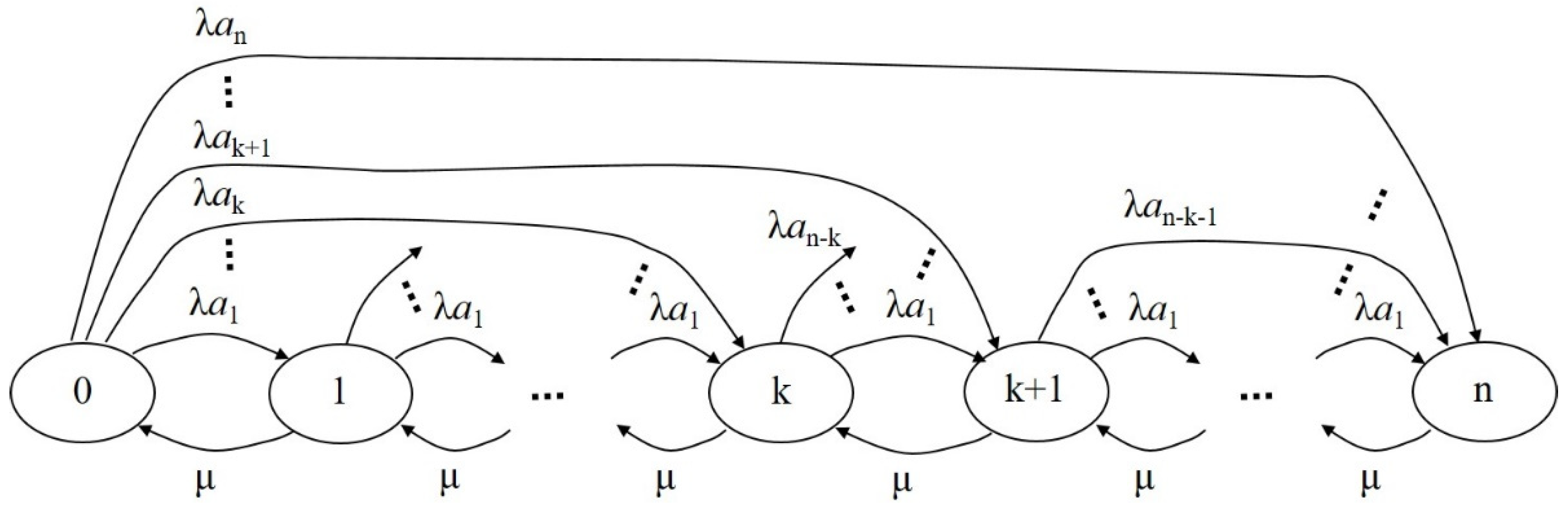
The notations of different arrival rates, time variables, and probabilities are listed in the nomenclature. The state of the system is determined by the number of customers in the system including the one in service. The state-transition diagram of the queueing model is shown in Figure 1. Let , 0 ≤ k ≤ n, be the probability that k customers are present in the system at time t. Then, the transient system equations can be described by the following first-order nonhomogeneous linear ODEs:
When the batch size X is a uniform random variable, the probability of different batch size will be equally probable, i.e., ai = a, 1 ≤ i ≤ n. By applying the normalization condition
the above ODEs can be re-written as follows.
It is observed that the above system, described by either ODEs (1)–(3) or ODEs (5)–(7), can be solved from the last ODE to the first with the obtained solutions applied to the solution of the next ODE. For the ease of presentation purpose, in the following we will focus the system solution on the ODEs (5)–(7).
3. Model Analysis and Solutions
In this section, we perform the analysis of the queueing model and derive the transient and steady state solutions to it. From the ODE (7), we have
By using the route ODE solving method [24], we obtain the solution of :
where the coefficient , and is a real constant determined by the initial condition of the ODE.
Consider the next ODE with k = n − 1 and re-write the ODE as
Substituting (9) into (10) and solve it as:
where the coefficients , i = 0, 1, 2, are real constants determined by the initial condition of the ODE.
Similarly, the rest ODEs in (6) are solved with the form:
where , 1 ≤ k ≤ n − 1, 0 ≤ i ≤ k + 1, are real constants determined by the initial condition of the ODEs.
Finally, substituting (12) into (5) and solving the ODE, we have
where , 0 ≤ i ≤ n + 1, are real constants determined by the initial condition of the ODEs.
Equations (9), (12) and (13) consist of the transient solution of the queueing system. The steady state system solution can be obtained when . Thus, the steady state probabilities are , .
In practice, the queueing system is usually empty in the beginning. Thus, the initial condition of the ODEs is:
By applying the initial condition of the system (14) to the transient solution of Equations (9), (12) and (13), we can recursively determine all the coefficients , , .
It can be easily shown that is equal to zero by substituting related expressions into Equation (22). After all the coefficients are solved, the transient solution to the queueing model will be obtained. The steady state solution to the model will also be obtained by letting t approach infinity.
4. Case Study
In this section, we present a case study for the proposed queueing model with n = 4 (i.e., one server and three waiting places). The queueing system can be re-written as follows.
The initial condition is:
The above queueing system can be solved as the Initial Value Problem (IVP) of ODEs. The solution is as follows.
where the coefficients are
It can be verified that the solution to the case study is consistent with the solution to the general queueing model described by Equations (9), (12) and (13) along with Equations (15) to (22). The corresponding steady state solution is given by , .
5. Performance Metrics
5.1. Blocking Probability of the System
The system blocking probability, denoted by PB(t), is equal to the probability that there are n customers in the system including the one in service, so the new arrival of customer has to be blocked. Thus, we have
5.2. Availability of the System
The availability of the system, denoted by AS(t), is defined as the probability that the system can accept at least one customer.
5.3. Idle and Busy Probabilities of the System
The system idle probability, denoted by PId(t), is defined as the probability that the system is empty (i.e., no customers in service and in the queue).
The system busy probability, denoted by PBu(t), is defined as the probability that there is at least one customer in the system.
5.4. Queueing Probability of the System
The system queueing probability, denoted by PQ(t), is defined as the probability that there is at least one customer in the queue.
5.5. Mean Number of Customers in the System and Queue
The mean number of customers in the system, NS(t), can be expressed as
Similarly, the mean number of customers in the queue, NQ(t), can be calculated as
5.6. Mean Waiting Time of Customers in the System and Queue
By Little’s law, the mean waiting time of customers in the system, denoted by WS(t), can be determined as
where is the effective arrival rate, i.e., the mean rate of the customers actually entering the system. As the system is finite and the arriving customers who find the system full leave the system, the effective arrival rate can be calculated as
Similarly, the mean waiting time of customers in the queue, denoted by WQ(t), can be determined as
6. Numerical Results
After obtaining the transient analysis (and thus the steady state analysis) of the finite queueing model and the developed performance metrics, we can apply them to many different fields such as healthcare, telecommunication, commerce, manufacturing, transportation, etc. However, we will leave these to our future study. Rather, in this section we present numerical results for the validation of our analytical solution under different parameters. The typical parameter settings are given in Table 1.
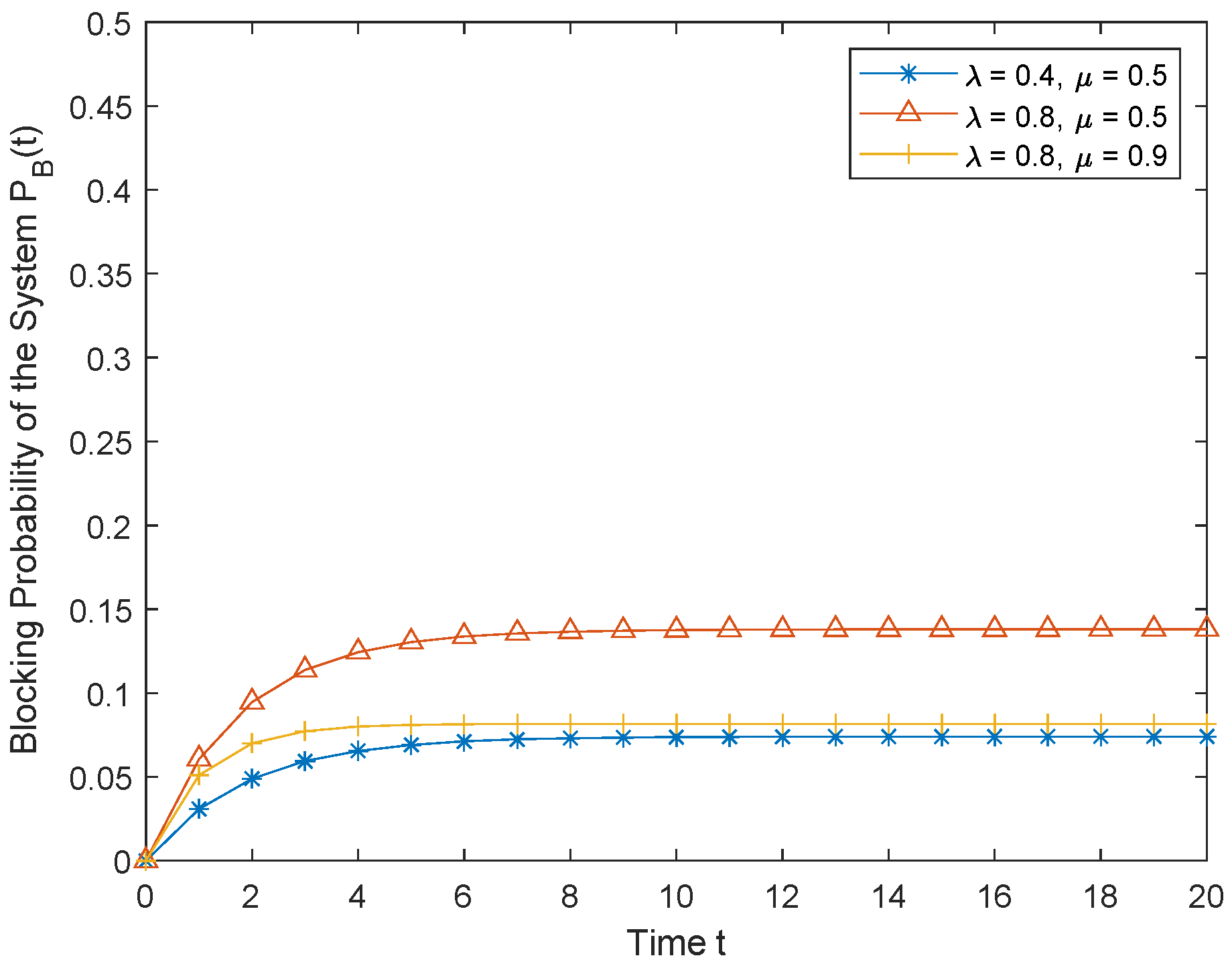
Figure 2 shows how the transient solution of the blocking probability PB(t) changes with respect to time t and the arrival and service rates λ and μ. The probability PB(t) will gradually increases and then tend to stabilize as the time goes. This is reasonable as more places are initially available for the arriving customers and gradually become less and less. We also observe that PB(t) will increase when the arrival rate (λ) or the service time (1/μ) is increased. The increase of the arrival rate will lead to more customers entering the queue and thus cause the system to tend to block. Equivalently, the increase of the service time will cause more customers to wait in the queue.
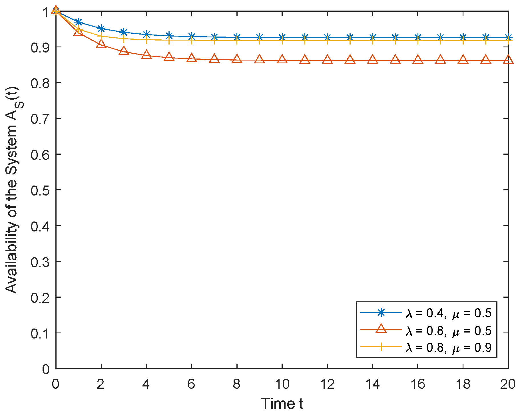
Figure 3 shows the transient solution of the system availability AS(t) with respect to time t and the arrival and service rates λ and μ. The availability AS(t) will gradually decreases and then tend to be constant with respect to time. The system will have more customers and thus less available as time goes. We also observe that AS(t) will decrease when the arrival rate (λ) or the service time (1/μ) is increased. The more customers in the system, the less availability for the system.
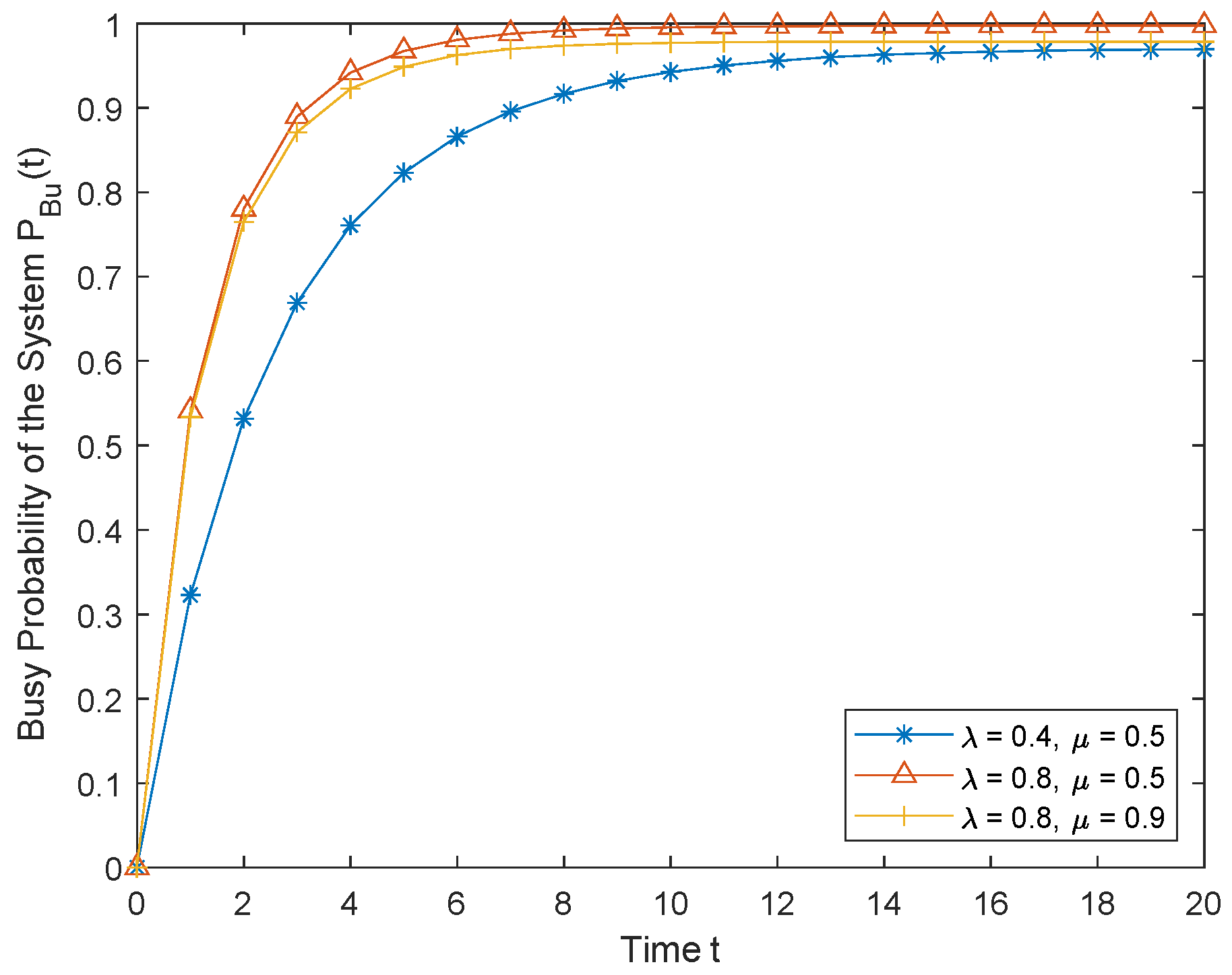
Figure 4 shows the busy probability of the system PBu(t) with respect to time and other parameters. As expected, PBu(t) will increase with respect to time as more and more customers arrive at the system and the system becomes busier. Similarly, when the arrival rate increases or the service rate reduces, PBu(t) will become busier.
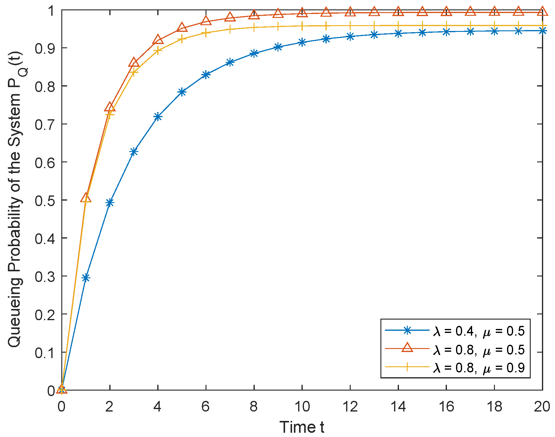
Figure 5 shows the queueing probability of the system PQ(t) with respect to time and other parameters. Similar to PBu(t), we observe that PQ(t) is zero in the beginning of time (i.e., t = 0) and will increase with respect to time. We also observe that PQ(t) will increase when λ is increased or μ is decreased. More customer arrivals or less service capability of the service station leads to a large queueing probability.
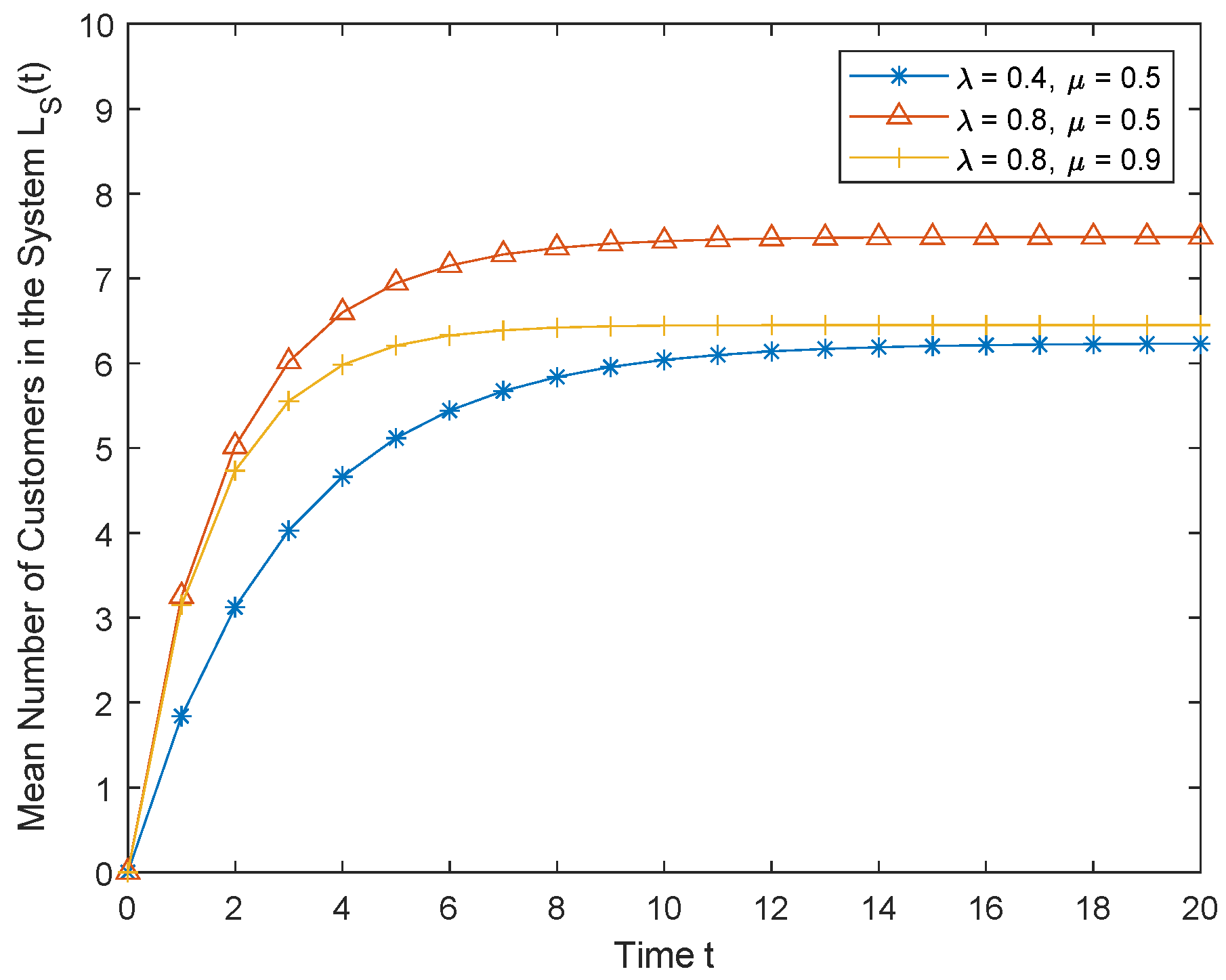
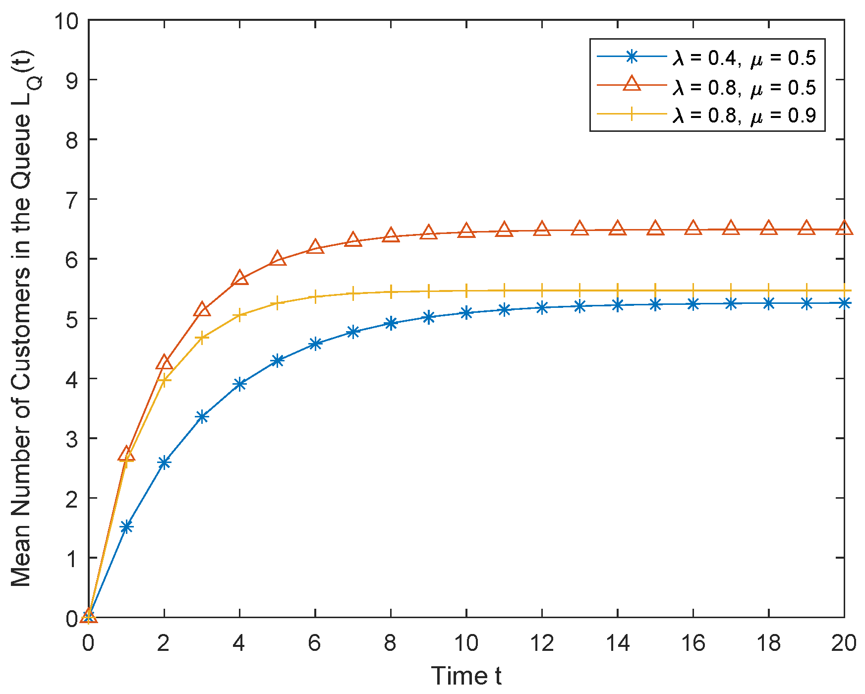
Figure 6 shows the mean number of customers in the system LS(t) with respect to time and arrival and service rates. We observe that LS(t) will increase with the increase of the arrival rate λ and the service time (1/μ). In a single server queueing system, it is obvious that the increase of the customer arrival rate will lead to the increase of the queueing length. Equivalently, the increase of the customer service time will cause more customers to wait in the queue and thus lead to the increase of queueing length. Similarly, the mean number of customers in the queue LQ(t) has the same characteristics, as shown in Figure 7.
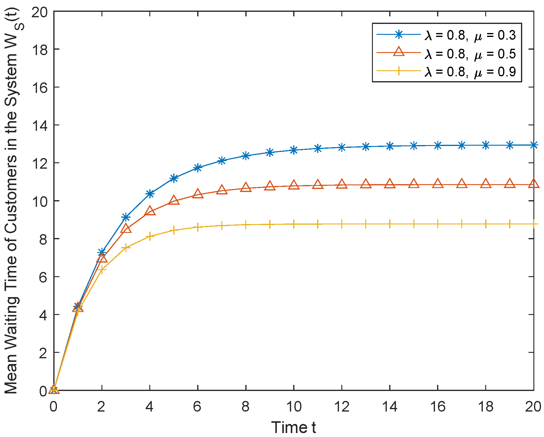
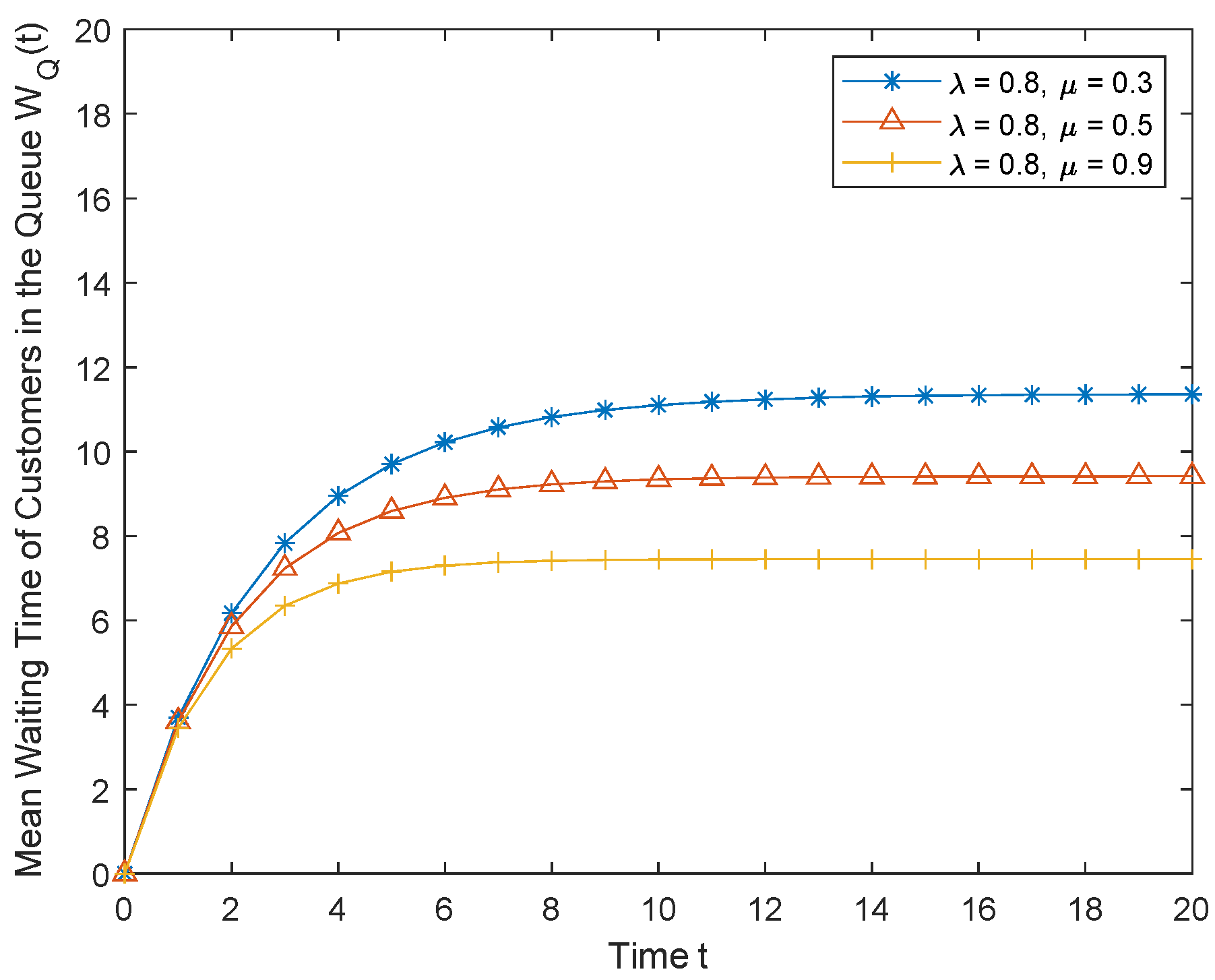
Figure 8 shows the mean waiting time of customers in the system WS(t) with respect to the change of time and service rate. We observe that WS(t) will increase with respect to time initially and then tends to stabilize as the time goes. We also observe that WS(t) will increase when the service rate is decreased. The decrease of service rate means the increase of service time per customer, leading to the increase of waiting time of other customers. The mean waiting time of customers in the queue WQ(t) has the same trend as WS(t) except with shorter time, as shown in Figure 9.
7. Conclusions
We proposed a finite capacity single server queueing model with bulk arrivals and performed the transient analysis for the system based on different system parameters. By using the ordinary differential equations (ODEs) technique, we derived the transient solution in explicit form for the queueing system and thus the steady state solution. A case study of the queueing model was presented for validation of the obtained transient solution. Some performance metrics of interest were then developed along with numerical results for further understanding. Our numerical results validated the analytical solutions of all the performance metrics including the transient solution of the blocking probability, the transient solution of the system availability, the busy probability of the system, the queueing probability of the system, the mean number of customers in the system and in the queue, and the mean waiting time of customers in the system and in the queue (Please refer the details in Section 6). Although the queueing model is initiated from the IoT based edge computing platform, the proposed system modeling and analysis method can be applied to a wider range of applications such as healthcare, telecommunication, commerce, manufacturing, transportation, etc.
Funding
This work was supported in part by the Faculty Improvement Grant (No. 211208) from Inter Faculty Organization (IFO)/Minnesota State Master Agreement, MN, USA.
Data Availability Statement
Not applicable.
Conflicts of Interest
The author declares no conflict of interest.
Nomenclature
| n | The total number of customers in the system. |
| k, 0 ≤ k ≤ n | The current number of customers in the system (i.e., the system state). |
| λ | The mean arrival rate of the bulk arrivals. |
| μ | The mean service rate of the single server system. |
| X | The random variable used to describe the number of arrivals in a group (i.e., batch size). |
| ai, 1≤ i ≤ n | The probability distribution of batch size, ai = P(X = i). |
| a | The probability of the batch size when the batch size X is a uniform random variable. |
| pk(t), 0 ≤ k ≤ n | The probability that k customers are present in the system at time t. |
| C(k, i) | The coefficients of the solution to the ODEs. |
| λ′ | The effective arrival rate. |
| PB(t) | The blocking probability of the system. |
| AS(t) | The system availability. |
| PId(t) | The system idle probability. |
| PBu(t) | The system busy probability. |
| PQ(t) | The system queueing probability. |
| LS(t) | The mean number of customers in the system. |
| LQ(t) | The mean number of customers in the queue. |
| WS(t) | The mean waiting time of customers in the system. |
| WQ(t) | The mean waiting time of customers in the queue. |
References
- Kleinrock, L. Queueing Systems, Volume 1: Theory, 1st ed.; Wiley-Interscience: Hoboken, NJ, USA, 1975. [Google Scholar]
- Chaudhry, M.L.; Templeton, J.G.C. A First Course in Bulk Queues; John Wiley & Sons: Hoboken, NJ, USA, 1983; ISBN 978-0471862604. [Google Scholar]
- Pegden, C.D.; Rosenshine, M. Some New Results for the M/M/1 Queue. Manag. Sci. 1982, 28, 821–828. [Google Scholar] [CrossRef]
- Lopez-Herrero, M.J. Distribution of the Number of Customers Served in an M/G/1 Retrial Queue. J. Appl. Probab. 2002, 39, 407–412. [Google Scholar] [CrossRef]
- Conolly, B.W. Queueing at a Single Serving Point with Group Arrival. J. R. Stat. Soc. Ser. B 1960, 22, 285–298. [Google Scholar] [CrossRef]
- Shanbhag, D.N. On Infinite Server Queues with Batch Arrivals. J. Appl. Probab. 1966, 3, 274–279. [Google Scholar] [CrossRef]
- Sharma, S.D. On a Continuous/Discrete Time Queueing System with Arrivals in Batches of Variable Size and Correlated Departures. J. Appl. Probab. 1975, 12, 115–129. [Google Scholar] [CrossRef]
- Alfa, A.S. A Numerical Method for Evaluating Delay to a Customer in a Time-Inhomogeneous, Single Server Queue with Batch Arrivals. J. Oper. Res. Soc. 1979, 30, 665–667. [Google Scholar] [CrossRef]
- van Dijk, N.M. An LCFS Finite Buffer Model with Finite Source Batch Input. J. Appl. Probab. 1989, 26, 372–380. [Google Scholar] [CrossRef]
- Choi, B.D.; Park, K.K. The Mk/m/∞ Queue with Heterogeneous Customers in a Batch. J. Appl. Probab. 1992, 29, 477–481. [Google Scholar]
- Chen, S.-P. A bulk arrival queueing model with fuzzy parameters and varying batch sizes. Appl. Math. Model. 2006, 30, 920–929. [Google Scholar] [CrossRef]
- Baruah, M.; Madan, K.C.; Eldabi, T. A Batch Arrival Single Server Queue with Server Providing General Service in Two Fluctuating Modes and Reneging during Vacation and Breakdowns. J. Probab. Stat. 2014, 2014, 319318. [Google Scholar] [CrossRef] [Green Version]
- Niranjan, S.P.; Indhira, K.; Chandrasekaran, V.M. Analysis of bulk arrival queueing system with batch size dependent service and working vacation. AIP Conf. Proc. 2018, 1952, 020061. [Google Scholar] [CrossRef]
- Laslett, G.M. Characterising the Finite Capacity GI/M/1 Queue with Renewal Output. Manag. Sci. 1975, 22, 106–110. [Google Scholar] [CrossRef]
- Chao, X. On the Departure Processes of M/M/1/N and GI/G/1/N Queues. Adv. Appl. Probab. 1992, 24, 751–754. [Google Scholar] [CrossRef] [Green Version]
- Kaczynski, W.H.; Leemis, L.M.; Drew, J.H. Transient Queueing Analysis. INFORMS J. Comput. 2012, 24, 10–28. [Google Scholar] [CrossRef] [Green Version]
- Kelton, W.D.; Law, A.M. The Transient Behavior of the M/M/s Queue, with Implications for Steady-State Simulation. Oper. Res. 1985, 33, 378–396. [Google Scholar] [CrossRef]
- Sharma, O.P.; Gupta, U.C. Transient Behaviour of an M/M/1/N queue. Stoch. Process. Appl. 1982, 13, 327–331. [Google Scholar] [CrossRef] [Green Version]
- Leguesdron, P.; Pellaumail, J.; Rubino, G.; Sericola, B. Transient Analysis of the M/M/1 Queue. Adv. Appl. Probab. 1993, 25, 702–713. [Google Scholar] [CrossRef] [Green Version]
- Sharmaand, O.P.; Tarabia, A.M.K. A Simple Transient Analysis of an M/M/1/N Queue. Sankhyā Indian J. Stat. Ser. A 2000, 62, 273–281. [Google Scholar]
- Garcia, J.-M.; Brun, O.; Gauchard, D. Transient Analytical Solution of M/D/1/N Queues. J. Appl. Probab. 2002, 39, 853–864. [Google Scholar] [CrossRef]
- Kaczynski, W.; Leemis, L.; Drew, J. Modeling and analyzing transient military air traffic control. In Proceedings of the 2010 Winter Simulation Conference, Baltimore, MD, USA, 5–8 December 2010; pp. 1395–1406. [Google Scholar] [CrossRef] [Green Version]
- Chydzinski, A.; Adamczyk, B. Transient and Stationary Losses in a Finite-Buffer Queue with Batch Arrivals. Math. Probl. Eng. 2012, 2012, 326830. [Google Scholar] [CrossRef]
- Kreyszig, E. Advanced Engineering Mathematics, 10th ed.; Wiley: Hoboken, NJ, USA, 2020; ISBN 978-1119455929. [Google Scholar]
Figure 1.
The single server queueing model with finite capacity and bulk arrivals.

Figure 2.
The blocking probability of the system PB(t).

Figure 3.
The system availability AS(t).

Figure 4.
The busy probability of the system PBu(t).

Figure 5.
The queueing probability of the system PQ(t).

Figure 6.
The mean number of customers in the system LS(t).

Figure 7.
The mean number of customers in the queue LQ(t).

Figure 8.
The mean waiting time of customers in the system WS(t).

Figure 9.
The mean waiting time of customers in the queue WQ(t).


Table 1.
Typical parameter configuration for numerical evaluation.
| Parameters | Value | Unit | Description |
|---|---|---|---|
| t | [0, 30] | General time units | time |
| λ | 0.4, 0.9 | Customers/unit time | arrival rate |
| μ | 0.5, 1.0 | Customers/unit time | service rate |
| n | 10 | Number of customers | system capacity |
| ai = a, i ≤ n | 0.1 | Prob. distribution of bulk arrivals |
Publisher’s Note: MDPI stays neutral with regard to jurisdictional claims in published maps and institutional affiliations. |
© 2022 by the author. Licensee MDPI, Basel, Switzerland. This article is an open access article distributed under the terms and conditions of the Creative Commons Attribution (CC BY) license (https://creativecommons.org/licenses/by/4.0/).
Share and Cite
MDPI and ACS Style
Tang, S. Transient Analysis of a Finite Queueing System with Bulk Arrivals in IoT-Based Edge Computing Systems. IoT 2022, 3, 435-449. https://doi.org/10.3390/iot3040023
AMA Style
Tang S. Transient Analysis of a Finite Queueing System with Bulk Arrivals in IoT-Based Edge Computing Systems. IoT. 2022; 3(4):435-449. https://doi.org/10.3390/iot3040023
Chicago/Turabian StyleTang, Shensheng. 2022. "Transient Analysis of a Finite Queueing System with Bulk Arrivals in IoT-Based Edge Computing Systems" IoT 3, no. 4: 435-449. https://doi.org/10.3390/iot3040023