Article

Fluctuations-Induced Quantum Radiation and Reaction from an Atom in a Squeezed Quantum Field

1
Department of Physics, University of Maryland, College Park, MD 20742, USA
2
Center for High Energy and High Field Physics, National Central University, Taoyuan 320317, Taiwan
3
Maryland Center for Fundamental Physics and Joint Quantum Institute, University of Maryland, College Park, MD 20742, USA
*
Author to whom correspondence should be addressed.
Physics 2023, 5(2), 554-589; https://doi.org/10.3390/physics5020040
Submission received: 13 March 2023 / Revised: 4 May 2023 / Accepted: 10 May 2023 / Published: 24 May 2023
(This article belongs to the Special Issue Vacuum Fluctuations)

Abstract

:
In this third of a series on quantum radiation, we further explore the feasibility of using the memories (non-Markovianity) kept in a quantum field to decipher certain information about the early universe. As a model study, we let a massless quantum field be subjected to a parametric process for a finite time interval such that the mode frequency of the field transits from one constant value to another. This configuration thus mimics a statically-bounded universe, where there is an ‘in’ and an ‘out’ state with the scale factor approaching constants, not a continuously evolving one. The field subjected to squeezing by this process should contain some information of the process itself. If an atom is coupled to the field after the parametric process, its response will depend on the squeezing, and any quantum radiation emitted by the atom will carry this information away so that an observer at a much later time may still identify it. Our analyses show that (1) a remote observer cannot measure the generated squeezing via the radiation energy flux from the atom because the net radiation energy flux is canceled due to the correlation between the radiation field from the atom and the free field at the observer’s location. However, (2) there is a chance to identify squeezing by measuring the constant radiation energy density at late times. The only restriction is that this energy density is of the near-field nature and only an observer close to the atom can use it to unravel the information of squeezing. The second part of this paper focuses on (3) the dependence of squeezing on the functional form of the parametric process. By explicitly working out several examples, we demonstrate that the behavior of squeezing does reflect essential properties of the parametric process. Actually, striking features may show up in more complicated processes involving various scales. These analyses allow us to establish the connection between properties of a squeezed quantum field and details of the parametric process which performs the squeezing. Therefore, (4) one can construct templates to reconstitute the unknown parametric processes from the data of measurable quantities subjected to squeezing. In a sequel paper these results will be applied to a study of quantum radiations in cosmology.

1. Introduction

This paper is the third of a series on quantum radiation, in the form of emitted radiation with an energy flux (distinct from thermal radiance felt by an accelerated atom, as in the Unruh effect [1]) from the internal degrees of freedom (idf) of an atom, tracing its origin to the vacuum fluctuations of a quantum field, including its backreaction on the idf dynamics of the atom, in the form of quantum dissipation. In Ref. [2], two of us considered how vacuum fluctuations in the field act on the idf of an atom (we may call this the ‘emitter’), modeled by a harmonic oscillator. We first showed how a stochastic component of the internal dynamics of the atom arises from the vacuum fluctuations of the field, resulting in the emittance of quantum radiation. We then showed how the backreaction of this quantum radiation induces quantum dissipation in the atom’s idf dynamics. We explicitly identified the different terms representing these processes in the Langevin equations of motion. Then, using the example of a stationary atom, we showed how, in this case, the absence of radiation at a far-away observation point where a probe (or detector—note the so-called Unruh-DeWitt ‘detector’ [1,3] is an emitter in the present context) is located is actually a result of complex cancellations of the interference between emitted radiation from the atom’s idf and the local fluctuations in the free field. By this, we pointed out that the entity which enters into the duality relation with vacuum fluctuations is not radiation reaction (in the quantum optics literature, e.g., [4,5,6,7], the relation between quantum fluctuations and radiation reaction is often mentioned without emphasizing the difference between classical radiation reaction [8,9] and quantum dissipation, which exist at two separate theoretical levels; only quantum dissipation enters in the fluctuations–dissipation relation with quantum fluctuations, not classical radiation reaction), which can exist as a classical entity, but quantum dissipation [10,11]. In the second paper [12], we considered the idf of the atom interacting with a quantum scalar field initially in a coherent state. We showed how the deterministic mean field drives the internal classical mean component to emit classical radiation and receive classical radiation reaction. Both components are statistically distinct and fully decoupled. It is clearly seen that the effects of the vacuum fluctuations of the field are matched with those of quantum radiation reaction, not with classical radiation reaction, as the folklore states, even promulgated in some textbooks. Furthermore, we identified the reason why quantum radiation from a stationary emitter is not observed, and a probe located far away only sees classical radiation.

1.1. Quantum Radiation from an Atom in a Squeezed Quantum Field

In this paper, we treat quantum radiation from an atom’s idf interacting with a quantum field in a squeezed state. The squeezed state is probably the most important quantum state, next to the vacuum state, with both rich theoretical meanings and broad practical applications, as well known in quantum optics (see, e.g., [13]). We are particularly interested in its role in cosmology of the early universe.

Quantum Field Squeezed by an Expanding Universe

Squeezed states of a quantum field are naturally produced in an expanding universe in fundamental processes which involve the parametric amplification of quantum fluctuations, such as particle creation [14,15], either spontaneous production from the vacuum or stimulated production from n-particle states, and structure formation [16] from quantum fluctuations of the inflaton field. From relics such as primordial radiation and matter contents observed today, with the help of theoretical models governing their evolution, one attempts to deduce the state of the early universe at different stages of development. In addition to particle creation and structure formation, we add here another fundamental quantum process, namely, quantum radiation. One can ask questions such as: If such radiation of a quantum nature is detected, how can one use it to reveal certain quantum aspects of the early universe? Uncovering secrets of the early universe by digging out information stored in the quantum field is in a similar spirit to the quest we initiated about the non-Markovianity of the universe through memories kept in the quantum field [17].

1.2. Three Components: Radiation, Squeeze, Drive

Towards such a goal we carry out this investigation which involves three components: (1) quantum radiation, (2) squeezed state, and (3) driven dynamics, either under some external force or as provided by an expanding universe, which describes how the squeeze parameter changes in time. Component (1) was initiated in Ref. [2] and continued in Ref. [12], where the required technical tools for the present investigation can be found. Component (2) is performed here: we consider a quantum field in a squeezed state with a fixed squeeze parameter, regarded as the end state of the quantum field after being squeezed under some drive protocol or cosmological evolution. For the description of squeezed states we follow the descriptions in our earlier paper [18]. Under the classification of the three types of squeezing described there, we adhere to the first type, namely, with fixed squeezing. The second type of dynamical parametric squeezing will be treated in our sequel cosmological papers. We set aside the third type of squeezing due to finite coupling between the system (here, the atom’s idf) and the environment (here, the quantum field) completely.
To see more explicitly what component (3) entails, consider a situation where the atom at the initial time t i is in a quantum field in a squeezed state with a fixed squeeze parameter ζ i and the same atom at the final time, t f , in a squeezed field with a different squeeze parameter, ζ f . If an atom emits quantum radiation at either or both the initial and the final times, comparing the signals from both should tell us something about how the drive had affected the atom through the quantum radiation emitted from the atom, or in cosmology, how the universe had evolved as measured by the parametric squeezing of the field. The more challenging situation is if it turns out that there is no emitted quantum radiation from an atom in a squeezed field. This is what our next work intends to find out.

1.3. Our Objectives, in Two Stages

We wish to ask questions in the same spirit as in Ref. [17]: Can we extract information about the history of the quantum field which had undergone a parametric process from the responses of an atom coupled to it in the epoch after the parametric process? In particular, for observers (receivers) situated far away from the atom (emitter), whether they can detect radiations emitted from the atom of a quantum nature. Quantum radiation is of special interest as it originates from the vacuum fluctuations of a quantum field, and is expected to keep some memories of the parametric process it went through. In a cosmological context, it acts as a carrier of quantum information about the early universe.
We divide our program of quantum radiation in cosmology into two stages, phrased as two questions. (A): Is there emitted quantum radiation from a stationary atom in a quantum field with a fixed squeeze parameter? If there is no emitted quantum radiation, then question (B): Is there emitted quantum radiation from a stationary atom in a quantum field subjected to a changing squeeze parameter, such as in an expanding universe? If so, what kind of evolutionary dynamics would produce what types of emitted radiation and with what magnitudes? The first stage addresses components (1) and (2) listed above, and the second stage, components (2) and (3), which will be continued in a follow-up paper.

1.3.1. Radiation Pattern as Template for Squeezing

This paper operates in the first stage, with a setup meant for a statically-bounded universe, not the continuously evolving type such as in the Friedmann–Lemaître–Robertson– Walker (FLRW) or the inflationary universe. The first half answers the first question (A), and the second half of this paper examines the response of the atom coupled to a field that had undergone a parametric process earlier. This evokes the template idea, i.e., one can use the response of the atom, coupled to the field in the out-region, to identify the dependence of the squeeze parameter on the earlier parametric process before the out-region. In the cosmology context, this offers a way for a late-time observer of such quantum phenomena to uncover how the universe had evolved in much earlier times.

1.3.2. Stress–Energy Tensor of Squeezed Field

To answer the central question (A), we use a simplified model in which the quantum field undergoes a parametric process of finite duration, such as under an external drive for a definite period of time, or in an asymptotically stationary (statically bounded) universe. The field could be a quantized matter or graviton field, or an inflaton field whose quantum fluctuations engender cosmological structures. Then, we calculate the expectation value of the stress–energy tensor of the radiation field emitted by an atom coupled to a free field in a fixed two-mode squeeze state. In order to identify the unambiguous signals and conform to the typical settings, we focus on the late-time results. We learned from our earlier invetsigation [2] for a quantum field in the vacuum state that the procedure for checking this is quite involved, as it entails both the radiation flux emitted from the atom as detected at the spacetime point of the probe, and an incoming flux from infinity.

1.4. Key Steps and Major Findings

The answer we found after calculating all relevant contributions for an atom in a quantum field in a squeezed state shows that there is no net radiation flux, the same as in Ref. [2]. This is a consequence of relaxation dynamics of the atom’s internal dynamics when it is coupled to the squeezed field [19]. However, if the probe can measure the radiation energy density, it should obtain a residual constant radiation energy density at late time. Its value will fall off similar to the inverse cubic power of the distance between the probe and the atom. Thus, it is more similar to a near-field effect. Nonetheless, this energy density has an interesting characteristic: it depends on the squeeze parameter, which is what we are after.
Thus, our investigation turns to whether and how the squeeze parameter of the field after the parametric process would depend on the details of the process. We first show that the squeeze parameter can formally be expressed by the fundamental solutions of the parametrically driven field; the latter contains useful information about the process. Then, by working out several examples numerically we can make the following observations:
(1)
For a monotonically varying process, the squeeze parameter has a monotonic dependence on the duration of this process; it does not depend on when the process starts, if we fix the duration.
(2)
The magnitude of squeezing is related to the rate of change in the process. That is, large squeezing can be induced from a nonadiabatic transition. This is consistent with our understanding of spontaneous particle creation from parametric amplification of vacuum fluctuations [20] and that copious particles can be produced at the Planck time under rapid expansion of the universe [21]. Thus, we expect that nonadiabatic processes may contribute to larger residual radiation energy density around the atom.
(3)
For a nonmonotonic parametric process, various scales in the process induce richer structure to the behavior of the squeeze parameter. In particular, if the parametric process changes with time sinusoidally at some frequency range, it may induce parametric resonance and yield exceptionally large squeezing in the out-region.
Similar considerations can likewise be applied to the frequency spectrum of the squeeze parameter of the field in the out-region. One can then examine its dependence on the parametric process which the field has undergone. This illustrates the way to obtain templates in how the squeeze parameter is related to the parametric process, and how certain information of the unknown parametric process can be inferred from these templates.

1.5. Organization

The paper is organized as follows. In Section 2, as a prerequisite, we briefly summarize our earlier results on the relaxation process of the atom–field interaction, and pose the questions we would like to answer in this paper. In Section 3, we lay out the formalism and the essential tools for detailing the nonequilibrium evolution of the atom’s internal dynamics and the squeezed field when they are coupled together. In Section 4, we study the general spatial–temporal behavior of the energy flux and the energy density of the radiation field and examine their late-time behaviors. In Section 5, we turn to the functional dependence of the squeeze parameter on the functional form of the parametric process. Several examples are provided to illustrate the formal analysis. In Section 6, we give some concluding remarks. Appendix A offers a succinct summary of the two-mode squeezed state. In Appendix B and Appendix C, we offer more details on the late-time, large-distance behaviors of the energy flux and the energy density of the radiation field. In Appendix D, we discuss the time-translational invariance of the squeeze parameter in the out-region.

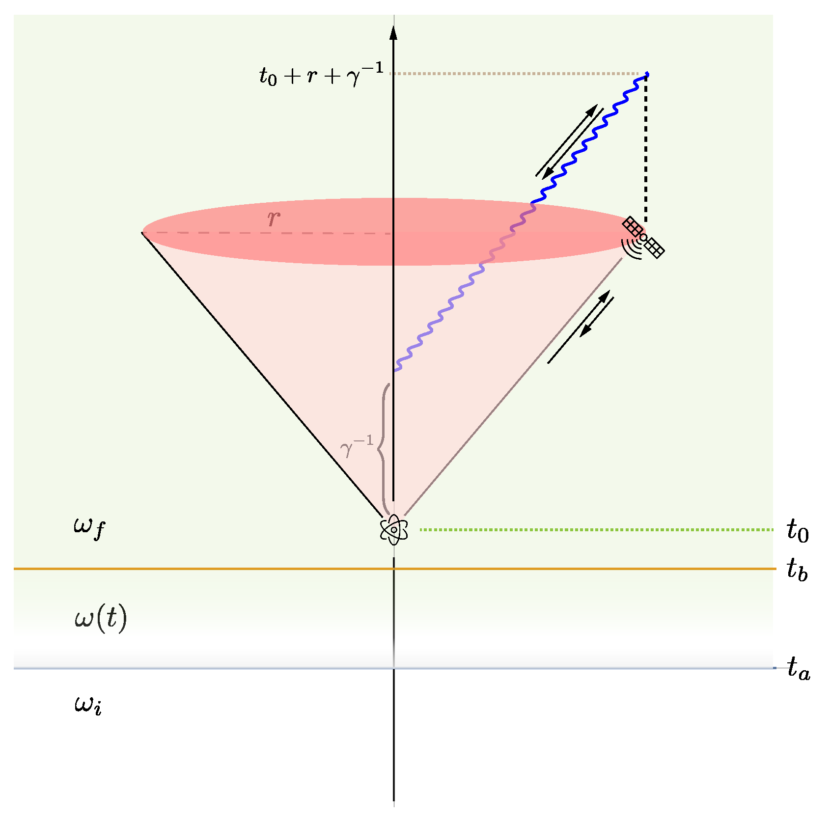
2. Scenario: Quantum Radiation in Atom–Field Systems

Classical radiation is a familiar subject, but what is its quantum field origin? Can one trace back its link all the way to quantum fluctuations? We obtained partial answers in our last two papers to this question for a harmonic atom interacting with a quantum field in a vacuum and in a coherent state. This paper deals with a squeezed field, necessary for treating cosmological quantum processes. Since fluctuation-induced quantum radiation is not a household topic, yet it might be useful to first provide a physical picture of the global landscape of quantum radiation based on our understanding from previous studies, setting the stage for the current paper.
It has been shown that [19] when the internal degree of freedom, modeled as a harmonic oscillator, of an atom (called a harmonic atom) in any initial state is linearly coupled to a massless linear scalar field in the stationary state, its motion will settle down to an equilibrium state. The presence of this equilibrium state, from the perspective of the atom, implies a balance of energy exchange between the atom and the environmental field. Expectantly, the radiation generated by the nonequilibrium motion of the atom’s internal degree of freedom propagates outward to spatial infinity. It is lesser known whether and how, from the perspective of the field, the radiation energy from the atom is balanced. In our previous study [2], we demonstrated that the correlation between the outward radiation field and the local free field at spatial infinity constitutes an inward energy flow to balance the outward radiation energy flow. Furthermore, this inward flux serves to supplement the needed energy around the atom for the field to drive the atom’s internal motion. Thus, we clearly see how energy flows from the atom to spatial infinity and then backflows to the atom. This is a consequence of the nonequilibrium fluctuation–dissipation relations [2,22] for the atom’s internal degree of freedom and the free field, which is a stronger condition than the conservation of energy. This point is better appreciated once we take the global view of the total system, composed of the atom and field. The entire system is closed and the total energy is conserved, but this does not guarantee that the energy exchange between two subsystems is balanced unless the reduced dynamics is fully relaxed to an equilibrium state.
If, instead, the internal degree of freedom of the atom is initially coupled to the quantum field in a nonstationary state, similar to the squeezed state, then will the nonstationary nature of the field prevent the internal degree of freedom from approaching an equilibrium state? We showed that [19] when the (mode-dependent) squeeze parameter is time-independent, the atom’s internal degree of freedom still settles down to an equilibrium state in the long run. The stationary components of the covariance matrix elements or the energy flows decay exponentially fast to time-independent constants as in the previous case, but the additional nonstationary components fall off to zero. The mechanisms that account for the late-time behavior of the stationary and the nonstationary components seem to be quite distinct. For the stationary components, it is a consequence of dissipation dynamically adapting to the driving fluctuations from the environment, but for the nonstationary components, cancellation due to fast phase variations in the nonstationary terms plays the decisive role. In contrast, from the viewpoint of the squeezed field, what is the nature of radiation emitted from the atom, and can this outward energy flux at distances far away from the atom find a corresponding inward flux at late times such that there is no net energy output to spatial infinity, as proven for the case of a stationary field? If so, what makes it possible?
These questions are of particular interest in a cosmological setting for the consideration of fundamental issues described in Section 1. There, evolution of the universe parametrically drives the ambient quantum field into a squeezed state. The extent of squeezing may depend on the characteristics of the parametric process actuated by the evolution of the background universe. When an atom is coupled to such a field, emitted radiation from the atom should carry the information of squeezing of the field, which in turn may reveal the evolution history of the universe.
As a prerequisite to addressing these issues, in this paper we are going to examine a simpler configuration that may cover the essential features. Consider, in Minkowski spacetime, a massless scalar field that undergoes a parametric process such that each mode frequency changes smoothly from one constant value, for example, ω i to another ω f , as shown in Figure 1. The parametric process occurs during the time interval t a t t b . In the out-region ( t t b ) of the process, an atom is coupled to the squeezed field at time t 0 . The nonequilibrium evolution of the internal degree of freedom of the atom then generates outward radiation, which after time r will reach a detector (such as a satellite around the Earth) at a distance r away from the atom. The detector may measure the time variation of the energy flux. The corresponding signal will be extracted and amplified to sieve out the information regarding the parametric process of the field occurred earlier.

3. Massless Scalar Field Interacting with a Harmonic Atom

For the case of a massless scalar field ϕ coupled to a static atom, with its internal degree of freedom, χ , represented by a harmonic oscillator, one has the following Heisenberg equations of motion:
χ ^ ¨ ( t ) + ω b 2 χ ^ ( t ) = e m ϕ ^ ( 0 , t ) ,
t 2 2 ϕ ^ ( x , t ) = e δ ( 3 ) ( x ) χ ^ ( t ) ,
where the atom is located at the origin of the spatial coordinates x in a 3 + 1 Minkowski spacetime. The parameter e denotes the coupling strength between the internal degree of freedom of the atom and the field, and ω b and m is the bare frequency and the mass of the oscillator, respectively. The overhead dot of a variable represents its time derivative with respect to t; if this variable is promoted to an operator, we add an overhead hat. δ ( 3 ) ( x ) is the three-dimensional delta function, and we often use the shorthand notation, a = / a , for the partial derivative with respect to a.
Solving the equation of motion of the field (2) yields
ϕ ^ ( x , t ) = ϕ ^ h ( x , t ) + e 0 t d s G R , 0 ( ϕ ) ( x , t ; 0 , s ) χ ^ ( s ) ,
where the homogeneous part ϕ ^ h ( x , t ) gives the free field while the integral expression represents the radiation field emitted by the atom. The retarded Green’s function G R , 0 ( ϕ ) ( x , x ) of the free field is defined by
G R , 0 ( ϕ ) ( x , x ) = i θ ( t t ) ϕ ^ h ( x ) , ϕ ^ h ( x ) = 1 2 π θ ( τ ) δ ( τ 2 R 2 ) ,
where x = ( x , t ) , τ = t t , R = | x x | , and θ ( τ ) is the Heaviside unit-step function. In the special case R 0 , which is met for a single Brownian oscillator, we instead have
G R , 0 ( ϕ ) ( t , t ) = 1 2 π θ ( τ ) δ ( τ ) .
Here, we suppressed the trivial spatial coordinates 0 , and the prime of a function denotes the derivative with respect to its argument. The superscript of the Green’s function indicates the operator by which the Green’s function is constructed, while the 0 in the subscript reminds us that the Green’s function of interest is associated with a free operator; otherwise it is an interacting operator. For example, G R , 0 ( ϕ ) ( τ ) refers to the retarded Green’s function of the free field, while G R ( χ ) ( τ ) is the retarded Green’s function of the interacting χ .
Plugging Equation (3) into the equation of motion (2) for the atom’s internal degree of freedom, one obtains:
χ ^ ¨ ( t ) + ω B 2 χ ^ ( t ) e 2 m 0 t d s G R , 0 ( ϕ ) ( t , s ) χ ^ ( s ) = e m ϕ ^ h ( 0 , t ) .
This is the generalized quantum Langevin equation for χ ^ ( t ) —it includes backreactions of the environmental field in terms of the noise force on the righthand side and the integral expression on the left hand side. As was identified in Equation (3), the latter is the reaction force due to emitted radiation, which retards the motion of the atom’s internal degree of freedom.
Supposing the free field has a Markovian spectrum, we can reduce Equation (6) into a local form:
χ ^ ¨ ( t ) + 2 γ χ ^ ˙ ( t ) + ω R 2 χ ^ ( t ) = e m ϕ ^ h ( 0 , t ) ,
and the oscillation frequency is renormalized to a physical value ω R . Since we want to examine the nature of radiation and its late-time behavior in relation to the atom’s internal dynamics in a self-consistent way, we need the field expression (3) written in terms of the solution to the equation of the reduced dynamics (7):
χ ^ ( t ) = χ ^ h ( t ) + e 0 t d s G R ( χ ) ( t s ) ϕ ^ h ( 0 , s ) ,
where the retarded Green’s function associated with χ ^ has the form
G R ( χ ) ( τ ) = 1 m Ω e γ τ sin Ω τ ,
with Ω = ω R 2 γ 2 , γ is the damping constant, and χ ^ h ( t ) is the homogeneous part. Equation (7) always implies that
d d t m 2 χ ^ ˙ ( t ) + m ω R 2 χ ^ 2 ( t ) = P ξ ( t ) + P γ ( t ) ,
where P ξ ( t ) is the power delivered by the free field fluctuations:
P ξ ( t ) = e 2 ϕ ^ h ( 0 , t ) , χ ˙ ( t ) ,
and P γ ( t ) represents the rate of energy lost due to dissipation:
P γ ( t ) = 2 m γ χ ˙ 2 ( t ) .
We showed [19] that even if the scalar field is initially in a nonstationary squeezed thermal state, the internal dynamics of the atom will still settle down to an asymptotic equilibrium state, where, in particular,
P ξ ( t ) + P γ ( t ) = 0 .
This is a stronger condition than Equation (10), which reflects energy conservation of the reduced dynamics.
From Equations (3) and (8), the full interacting field is then given by
ϕ ^ ( x ) = ϕ ^ h ( x ) + e 0 t d t G R , 0 ( ϕ ) ( x , t ; 0 , t ) χ ^ h ( t ) + e 0 t d s G R ( χ ) ( t s ) ϕ ^ h ( 0 , s ) .
It turns out convenient to split the full interacting field into three physically distinct components, ϕ ^ ( x ) = ϕ ^ h ( x ) + ϕ ^ T R ( x ) + ϕ ^ B R ( x ) , with
ϕ ^ T R ( x ) = e 0 t d t G R , 0 ( ϕ ) ( x , t ; 0 , t ) χ ^ h ( t ) ,
ϕ ^ B R ( x ) = e 2 0 t d t G R , 0 ( ϕ ) ( x , t ; 0 , t ) 0 t d s G R ( χ ) ( t s ) ϕ ^ h ( 0 , s ) ,
where ϕ ^ T R ( x ) is the transient term associated with the atom’s transient internal dynamics and ϕ ^ B R ( x ) is the backreaction field correlated with ϕ ^ h ( x ) everywhere.

Hadamard Function

At this point, we have not specified the state of the field. For the reason that is explained in Section 5, we assume that the initial state of the field the atom interacts with is a time-independent two-mode squeezed thermal state, for which the field’s density matrix has the form
ρ ^ TMST = k S ^ 2 ( ζ k ) ρ ^ β S ^ 2 ( ζ k )
where ρ ^ β is the thermal density matrix of the free field at temperature T B = β 1 , and S ^ 2 ( ζ k ) is the two-mode squeeze operator, with the squeeze parameter, ζ k = η k e i θ k , defined by
S ^ 2 ( ζ k ) = exp ζ k * a ^ + k a ^ k ζ k a ^ + k a k .
Here, the † sign denotes the hermitian conjugate, η k 0 , 2 π > θ k 0 , and k is the wave vector. For convenience, we collected the essential properties of the two-mode squeezed state in Appendix A. Here, we assume that the squeeze parameter is mode-independent to simplify the arguments.
If the free field has the plane-wave expansion,
ϕ ^ h ( x ) = d 3 k ( 2 π ) 3 2 1 2 ω a ^ k e i k · x + a ^ k e i k · x ,
with k · x = ω t + k · x , k = ( ω , k ) , and ω = | k | , then the free field’s Hadamard function for this two-mode squeezed thermal state has the form,
G H , 0 ( ϕ ) ( x , x ) = d 3 k ( 2 π ) 3 1 4 ω coth β ω 2 e i k · ( x x ) cosh 2 η e i ω ( t t ) sinh 2 η e i θ e i ω ( t + t ) + C . C . .
Here, “C.C.” represents the complex conjugate term. After carrying out the angular integration, one arrives at the following decomposition:
G H , 0 ( ϕ ) ( x , x ) = G H , 0 ( ϕ ) , ST ( x , x ) + G H , 0 ( ϕ ) , NS ( x , x ) ,
with
G H , 0 ( ϕ ) , ST ( x , x ) = d ω 2 π cosh 2 η coth β ω 2 sin ( ω | x x | ) 4 π | x x | e i ω ( t t ) ,
G H , 0 ( ϕ ) , NS ( x , x ) = 0 d ω 2 π sinh 2 η coth β ω 2 sin ( ω | x x | ) 4 π | x x | e i ω ( t + t ) + i θ + C . C .
Observe that the Hadamard function has an extra component that is not invariant under time translation, so we call it the nonstationary component of the Hadamard function. This is distinct from the case we consider in Ref. [2]. The emergence of this component is a consequence of the field being squeezed. We discuss its dynamical origin in Section 5. This nonstationary nature of the free field’s Hadamard function will impact on the dynamical evolution of the atom’s internal dynamics because the Hadamard function governs the statistics of the noise force sourcing (6), which naturally raises the concern as to whether the internal dynamics can ever equilibrate. As was mentioned earlier, it turns out the atom’s internal motion can still relax to an equilibrium, meaning a time-translation-invariant state. Details of derivations and discussions on this point can be found in Ref. [19].
Equations (20) or (21) are the essential ingredient used to express the Hadamard function G H ( ϕ ) ( x , x ) of the interacting field, which is needed to evaluate the stress–energy tensor. Following the decomposition (15), the interacting field’s Hadamard function is given by
G H ( ϕ ) ( x , x ) = 1 2 ϕ ^ h ( x ) , ϕ ^ h ( x ) + 1 2 ϕ ^ h ( x ) , ϕ ^ BR ( x ) + ϕ ^ BR ( x ) , ϕ ^ h ( x ) + 1 2 ϕ ^ BR ( x ) , ϕ ^ BR ( x ) + 1 2 ϕ ^ TR ( x ) , ϕ ^ TR ( x ) ,
where
1 2 ϕ ^ h ( x ) , ϕ ^ h ( x ) = G H , 0 ( ϕ ) ( x , x ) ,
1 2 ϕ ^ h ( x ) , ϕ ^ BR ( x ) = e 2 0 t d s 1 G R , 0 ( ϕ ) ( x , t ; 0 , s 1 ) 0 s 1 d s 2 G R ( χ ) ( s 1 s 2 ) G H , 0 ( ϕ ) ( x , t ; 0 , s 2 ) ,
1 2 ϕ ^ BR ( x ) , ϕ ^ BR ( x ) = e 4 0 t d s 1 0 t d s 1 G R , 0 ( ϕ ) ( x , t ; 0 , s 1 ) G R , 0 ( ϕ ) ( x , t ; 0 , s 1 ) × 0 s 1 d s 2 0 s 1 d s 2 G R ( χ ) ( s 1 s 2 ) G R ( χ ) ( s 1 s 2 ) G H , 0 ( ϕ ) ( 0 , s 2 ; 0 , s 2 ) ,
1 2 ϕ ^ TR ( x ) , ϕ ^ TR ( x ) = e 2 2 0 t d s 0 t d s G R , 0 ( ϕ ) ( x , t ; 0 , s ) G R , 0 ( ϕ ) ( x , t ; 0 , s ) χ ^ h ( s ) , χ ^ h ( s ) .
The second group inside the square brackets in Equation (24) is of special interest because it describes the correlation between the radiation field and the free field at any location outside the atom. We do not see such counterpart in classical electrodynamics because in classical field theory, there is no vacuum state to establish any correlation with the radiation field. Here, the correlation must be present because (1) the internal dynamics of the atom, which emits the radiation, is driven by the free field at the atom’s location and (2) the free field has nonvanishing correlation among any spacetime interval. Note that we are in the Heisenberg picture, so the expectation values are evaluated with respect to the initial state of both subsystems. The contribution in Equation (28) can be ignored at late times due to its transient nature. In addition, we also note that these four components are at most linearly proportional to G H , 0 ( ϕ ) ( x , x ) . Thus, at least before t r γ 1 , where r = | x | , the interaction field is expected to behave similar to a squeezed field to some extent.
For later convenience, we introduce a shorthand notation for an expression which comes up frequently:
L ω ( x , t ) = 0 t d s 1 G R , 0 ( ϕ ) ( x , t s 1 ) 0 s 1 d s 2 G R ( χ ) ( s 1 s 2 ) e i ω s 2 .
After we carry out the integrations, we find its explicit form is given by
L ω ( x , t ) = θ ( t r ) G ˜ R ( χ ) ( ω ) G ˜ R , 0 ( ϕ ) ( x ; ω ) e i ω t e γ ( t r ) 4 π Ω r ( ω + i γ ) cos Ω ( r t ) + i Ω sin Ω ( r t ) ,
where we used the identity for the Fourier transform of G R , 0 ( ϕ ) ( x , τ ; 0 , 0 ) :
G ˜ R , 0 ( ϕ ) ( x ; ω ) = e i ω r 4 π r .
The convention of the Fourier transformation we adopt is
f ( t ) = d ω 2 π f ˜ ( ω ) e i ω t .
At times t r , we find that the dominant term in Equation (30) is given by
L ω ( x , t ) = θ ( t r ) G ˜ R ( χ ) ( ω ) G ˜ R , 0 ( ϕ ) ( x ; ω ) e i ω t ,
because in this case, the factor e γ ( t r ) causes the second term in the curly brackets in Equation (30) to be exponentially small. These are convenient snippets that greatly simplifies the analysis of the late-time behavior of the expectation values of the energy–momentum stress tensor of the interacting field. Henceforth, we proceed with the analysis separately for the contributions due to the stationary and the nonstationary components of G H , 0 ( ϕ ) ( x , x ) .
At late times, the explicit expressions for the stationary and nonstationary components of the Hadamard functions of the free field and the interacting field ϕ become relatively simple. The interacting field’s Hadamard function can likewise be decomposed into a stationary and a nonstationary component, G H ( ϕ ) ( x , x ) = G H ( ϕ ) , ST ( x , x ) + G H ( ϕ ) , NS ( x , x ) , and
G H ( ϕ ) , ST ( x , x ) = G H , 0 ( ϕ ) , ST ( x , x ) + e 2 d ω 2 π G ˜ H , 0 ( ϕ ) , ST ( x , 0 ; ω ) G ˜ R ( χ ) * ( ω ) G ˜ R , 0 ( ϕ ) * ( x ; ω ) + G ˜ H , 0 ( ϕ ) , ST ( x , 0 ; ω ) G ˜ R ( χ ) ( ω ) G ˜ R , 0 ( ϕ ) ( x ; ω ) e i ω ( t t ) + C . C . + e 2 d ω 2 π cosh 2 η coth β ω 2 G ˜ R , 0 ( ϕ ) ( x , ω ) G ˜ R , 0 ( ϕ ) * ( x , ω ) Im G ˜ R ( χ ) ( ω ) e i ω ( t t ) + C . C . ,
and
G H ( ϕ ) , NS ( x , x ) = G H , 0 ( ϕ ) , NS ( x , x ) e 2 0 d ω 2 π sinh 2 η coth β ω 2 G ˜ R ( χ ) ( ω ) × sin ( ω | x | ) 4 π | x | G ˜ R , 0 ( ϕ ) ( x ; ω ) + sin ( ω | x | ) 4 π | x | G ˜ R , 0 ( ϕ ) ( x ; ω ) e i ω ( t + t ) + i θ + C . C . e 4 0 d ω 2 π ω 4 π sinh 2 η coth β ω 2 G ˜ R ( χ ) 2 ( ω ) G ˜ R , 0 ( ϕ ) ( x ; ω ) G ˜ R , 0 ( ϕ ) ( x ; ω ) e i ( ω ( t + t ) + i θ + C . C . ,
where
G ˜ H , 0 ( ϕ ) , ST ( x , 0 ; ω ) G ˜ H , 0 ( ϕ ) , ST ( x ; ω ) = cosh 2 η coth β ω 2 sin ( ω | x | ) 4 π | x | = cosh 2 η coth β ω 2 Im G ˜ R , 0 ( ϕ ) ( x ; ω ) .
The energy–momentum stress tensor of the interacting field is then constructed via the Hadamard function, G H ( ϕ ) ( x , x ) . Analyses of the late-time energy flow of the field at distances far away from the atom resulting from the atom–field interaction are contained in Appendix B and Appendix C. A general discussion of the spatial–temporal behavior of the stress–energy tensor due to the radiation field emitted from the atom follows in the next section.

4. Stress–Energy Tensor Due to the Radiation Field

The expectation value of the energy–momentum stress tensor due to the radiation field is defined by
Δ T ^ μ ν ( x ) = lim x x 2 x μ x ν 1 2 g μ ν g α β 2 x α x β G H ( ϕ ) ( x , x ) G H , 0 ( ϕ ) ( x , x )
with the signature of the metric g μ ν being ( , + , + , + ) . Here, we subtracted off the contribution purely from the free field, which is irrelevant to the atom–field interaction. Due to symmetry, it has no dependence on the azimuthal angle, ϑ , and the polar angle, φ , of the spherical coordinate system, so the stress–energy tensor already reduces to
Δ T ^ μ ν = Δ T ^ t t Δ T ^ t r 0 0 Δ T ^ r t Δ T ^ r r 0 0 0 0 0 0 0 0 0 0 .
Then, we focus on the components Δ T ^ t r and Δ T ^ t t that are relevant to our following discussions.
Here, the analysis is not limited to the large-distance and the late-time limits, so that we can have a more complete, global view of the energy flow and energy density of the field caused by the atom–field interaction. We will place the analysis in those specific regimes in Appendix B and Appendix C.
Since in our configuration the coupling between the harmonic atom and the massless scalar field takes a different form from that between the point charge and the electromagnetic fields, it would be more illustrative if we first quickly cover the elementary derivations of the continuity equation and the total atom–field Hamiltonian in the classical regime to highlight their differences.
From the equation of motion of the scalar field (2), if we multiply both sides by t ϕ , we obtain a local form of the continuity equation
t u ϕ + · S ϕ = p t ϕ ,
where p ( x , t ) = e δ ( 3 ) ( x ) χ ( t ) serves as the point dipole associated with the atom, and we identify the field energy density, u ϕ , and the field momentum density, S ϕ , respectively, by
u ϕ ( x , t ) = 1 2 t ϕ ( x , t ) 2 + 1 2 ϕ ( x , t ) 2 , S ϕ ( x , t ) = t ϕ ( x , t ) ϕ ( x , t ) .
The unusual issue with the right hand side of the continuity Equation (39) is best appreciated when we compare with the corresponding equation for the electromagnetic fields:
t u + · S = J · E , with u = 1 2 E 2 + 1 2 B 2 , S = E × B ,
where J is the current density and the corresponding current is equal to e x ˙ for a point charge at the location x . The electric field, E , is defined by E = A 0 t A and the magnetic field B by B = × A . Here, A 0 is the scalar potential and A is the vector potential. Thus, the right hand side of Equation (39) should bear a similar interpretation to J · E , which is usually understood as the dissipation of the field energy due to the work performed by the field on the charge. That is, it is the opposite of the power delivered by the Lorentz force. However, there are a few subtle catches: (1) In classical field theory, we seldom consider the free field component of the field equation, and we never have vacuum field fluctuations, so the electromagnetic fields in Equation (41) are often assumed to be the field generated by the charge. In contrast, the quantum scalar field ϕ under our consideration is a full interacting field, comprising the free field and the radiation field emitted by the atom. Thus, the right hand side of Equation (39) will contain an extra contribution associated with the free field fluctuations. (2) The right hand side of Equation (39) does not correspond to the net power delivered by the field to the internal degree of freedom of the atom, which is e ϕ ( 0 , t ) t χ ( t ) , apart from a renormalization contribution, according to the right hand side of Equation (1). Then the interpretation of the right hand of Equation (39) is not so straightforward, even though it has a form of the dipole interaction, similar to the right hand side of Equation (41).
We may trace such a feature to the Hamiltonian. The Hamiltonian H χ ϕ associated with the Lagrangian of the atom–field interacting system,
L χ ϕ = m 2 χ ˙ 2 m ω B 2 2 χ ˙ 2 + V d V e δ ( x ) χ ( t ) ϕ ( x , t ) + V d 3 x 1 2 t ϕ ( x , t ) 2 1 2 ϕ ( x , t ) 2 ,
under our consideration is given by
H χ ϕ = m 2 χ ˙ 2 + m ω B 2 2 χ ˙ 2 e χ ( t ) ϕ ( 0 , t ) + V d 3 x 1 2 t ϕ ( x , t ) 2 + 1 2 ϕ ( x , t ) 2 ,
where we implicitly assume that χ ˙ ( t ) and ϕ ˙ ( x , t ) are functions of the respective canonical momenta, p ( t ) and π ( x , t ) . The quantity V denotes the whole spatial volume on a fixed time slice. Since the whole atom–field system forms a closed system, the total energy is conserved, so one has d H / d t = 0 ,
d d t H χ ϕ ( t ) = 0 = χ ˙ ( t ) m χ ¨ ( t ) + m ω B 2 χ ( t ) e ϕ ( 0 , t ) + V d 3 x e δ ( x ) χ ( t ) t ϕ ( x , t ) + d d t 1 2 t ϕ ( x , t ) 2 + 1 2 ϕ ( x , t ) 2 .
Note how the derivative of the interaction term is distributed, and further observe that the contribution inside of the first pair of curly brackets gives zero, following the equation of motion (1). It actually has an attractive interpretation. Following the derivations of Equations (6) and (7), it accounts for the reduced dynamics of the atom’s internal degree of freedom, and, from the atom’s perspective, describes the energy exchange between the atom and the surrounding quantum field.
The integral on the right hand side of Equation (44), on the other hand, describes the energy exchange from the field’s perspective, and thus gives zero too. In the integrand, we see the presence of the same dipole interaction term e δ ( x ) χ ( t ) t ϕ ( x , t ) that appears on the right hand side of Equation (39). At first sight, it may seem odd that the dipole interaction term is solely responsible for the change of the field energy; however, we can further show that
d d t H χ ϕ ( t ) = 0 = V d 3 x · [ ϕ ( x , t ) t ϕ ( x , t ) ] = V d A · S ( x , t ) ,
where d A is the area element on the boundary V . It says that there is no flux entering from or leaving to spatial infinity because the boundary V of the space volume V lies at spatial infinity. It is a rephrase of energy conservation in a closed system, so there is no inconsistency. On the other hand, Equation (45) is too restrictive because V is the total volume. The differential form of the continuity Equation (39) is more suitable to observe the energy distribution in the field.
In contrast to Equation (43), the Hamiltonian for the interacting system of a point charge and the electromagnetic field is
H x A = m B 2 x ˙ 2 + m B ω 2 2 x 2 + 1 2 V d 3 x E 2 + B 2 .
It does not have the interaction term manifestly if the Hamiltonian is not expressed in terms of the canonical momentum of the charge; however, it is consistent with the observation that J · E is opposite to the power delivered by the Lorentz force.
Now, let us discuss the general result of Δ T ^ μ ν that will be valid for t > r at any location distance r away from the atom, so we come back to the manipulation of quantum operators. We first compute Δ T ^ t r .

4.1. General Behavior of Field Energy Flux Δ T ^ t r

If we write ϕ ^ R ( x , t ) as
ϕ ^ R ( x , t ) = e 0 t d s G R , 0 ( ϕ ) ( x , t ; 0 , s ) χ ^ ( s ) = e 4 π r θ ( t r ) χ ^ ( t r ) ,
which explicitly shows that the radiation field is a retarded Coulomb-like field emitted by a source at an earlier time t r . Note that the quite simple expression of the radiation field such as Equation (47) is not obtainable if the field has a nonMarkovian spectrum.
With the help of Equation (47), one obtains:
1 2 t ϕ ^ R ( x , t ) , r ϕ ^ R ( x , t ) = e 4 π r 2 χ ^ 2 ( t r ) e 4 π r 2 1 2 r χ ^ ( t r ) , χ ^ ( t r ) ,
for t > r , where a prime denotes taking the derivative with respect to the function’s argument. If we compute the energy flow associated (48), across any spherical surface of radius r centered at the atom, we obtain
V d A 1 2 t ϕ ^ R ( x , t ) , r ϕ ^ R ( x , t ) = 2 m γ χ ^ 2 ( t r ) m γ r χ ^ ( t r ) , χ ^ ( t r ) = P γ ( t r ) m γ r t χ ^ 2 ( t r ) ,
where we used the substitution e 2 = 8 π γ m . The first term has a special significance. From Refs. [2,18,22], one knows that P γ ( t ) is the energy that the atom’s internal degree of freedom loses to the surrounding field due to damping. Thus, the first term tells us that the energy lost by the atom at time t r takes time r to propagate to a location at a distance r away from the atom. It is the only contribution in Equation (49) that may survive at spatial infinity.
The contribution from the cross-terms need a little more algebraic manipulations, but it gives:
1 2 t ϕ ^ h ( x , t ) , r ϕ ^ R ( x , t ) + 1 2 t ϕ ^ R ( x , t ) , r ϕ ^ h ( x , t ) = 1 4 π r 2 P ξ ( t r ) e 2 4 π r 2 t 0 t r d s G R ( χ ) ( t r s ) G H , 0 ( ϕ ) ( x , t ; 0 , s ) ,
in which the integral in the last expression is nothing but
e 2 0 t r d s G R ( χ ) ( t r s ) G H , 0 ( ϕ ) ( x , t ; 0 , s ) = e 2 χ ^ ( t r ) , ϕ ^ h ( x , t ) .
Here, P ξ ( t ) is the power that the free quantum field fluctuations deliver to the atom’s internal dynamics at time t at the atom’s location. Then we find the incoming energy flow given by
V d A 1 2 t ϕ ^ h ( x , t ) , r ϕ ^ r ( x , t ) + 1 2 t ϕ ^ r ( x , t ) , r ϕ ^ h ( x , t ) = P ξ ( t r ) t e 2 χ ^ ( t r ) , ϕ ^ h ( x , t ) .
Combining Equations (49) and (52), one thus has:
Δ T ^ t r = 1 4 π r 2 P ξ ( t r ) + P γ ( t r ) t m γ r χ ^ 2 ( t r ) + e 2 χ ^ ( t r ) , ϕ ^ h ( x , t ) ,
From the relaxation of the reduced dynamics of the atom’s internal degree of freedom, outlined in the beginning of Section 3, we learn that the internal dynamics will reach equilibrium, where P ξ ( t ) + P γ ( t ) = 0 for t γ 1 . Hence, from Equation (53), we easily conclude that, for a fixed r, when t r is much greater than the relaxation time scale, the sum of the dominant terms P ξ ( t r ) + P γ ( t r ) vanishes. At large distances away from the atom, the remaining terms are quite small, decaying at least similar to 1 / r 3 . It is consistent with our results in Appendix B, where we explicitly show that they actually give zero at late times. Alternatively, we may deduce the same conclusion here, since (1) χ ^ 2 ( t ) will approach a constant at late times as the atom’s internal dynamics asymptotically reach an equilibrium, and (2) with the help of the explicit expression,
e 2 χ ^ ( t r ) , ϕ ^ h ( x , t ) = e 2 4 π r 0 d ω 2 π coth β ω 2 cosh 2 η 0 t r d s G R ( χ ) ( t r s ) sin ω r 4 π r 2 cos ω ( t s ) ,
it is not hard to see that the time derivative of the last term inside the square brackets in Equation (53) vanishes at late times.
Thus, the detector away from the atom will not measure any radiation energy flux from the stationary atom at late times even though the atom is coupled to a nonstationary squeezed state.

4.2. General Behavior of Field Energy Density Δ T ^ t t

It is also of interest to examine the change of the field energy density at distances far away from the atom resulting from their mutual interactions. Conceptually, the atom’s internal dynamics will send out spatial infinity spherical waves centered at the location of the atom. Due to the quantum nature of the internal dynamics, this radiation wave, in general, has a random phase and its magnitude is inversely proportional to the distance to the atom. Following our previous discussion, a detector at a large but fixed distance away from the atom will receive a net outward energy flux in the beginning, and then it will find that the magnitude of the flux rapidly falls off to zero with time. After all these activities settle down, will the earlier energy flux leave any footprint in the space surrounding the atom, say, by shifting the local field energy density, albeit almost imperceptibly? This is what we try to find out in this section.
In the same manner, we rewrite Δ T t t , following Equation (47). Other than the overall factor 1 / 2 , we first show:
1 2 t ϕ ^ R ( x , t ) , t ϕ ^ R ( x , t ) + 1 2 r ϕ ^ R ( x , t ) , r ϕ ^ R ( x , t ) = 2 × 1 4 π r 2 P γ ( t r ) + r m γ r χ ^ 2 ( t r ) ,
where t χ ( t r ) = r χ ( t r ) . Here, due to the minus sign up front, this contribution tends to grow to a positive value at late times. We further note that the same expression P γ ( t r ) also appears in the component (49) of Δ T ^ t r ( t ) that is purely caused by the radiation field. Thus, we see the outward energy flux due to Equation (49) that imparts field energy into the space around the atom.
For the cross-terms, we obtain:
2 × 1 2 t ϕ ^ h ( x , t ) , t ϕ ^ R ( x , t ) + 2 × 1 2 r ϕ ^ h ( x , t ) , r ϕ ^ R ( x , t ) = 2 × 1 4 π r 2 P ξ ( t r ) + r e 2 χ ^ ( t r ) , ϕ ^ h ( x , t ) .
Following the same argument, the inward energy flux from Equation (50), on the other hand, is prone to take away the field energy in the surrounding space.
Altogether, we thus find that the net field energy density outside the atom is given by
Δ T ^ t t = 1 4 π r 2 P ξ ( t r ) + P γ ( t r ) + r m γ r χ ^ 2 ( t r ) + e 2 χ ^ ( t r ) , ϕ ^ h ( x , t ) ,
for t > r > 0 . This looks similar to Equation (53), and can be the consequence of the continuity equation. The dominant term in Equation (55) will vanish at late times, as a consequence of the relaxation of the internal dynamics of the atom, and the behavior of Equation (53) due to the appearance of t r . Following our earlier arguments, the remaining term, χ ^ ( t r ) , ϕ ^ h ( x , t ) , on the other hand, becomes a time-independent constant at late times, which falls off at least similar to 1 / r 3 , as is explicitly shown in Appendix B.2.
Indeed, Equations (53) and (55) enable us to verify the continuity equation,
1 r 2 r r 2 Δ T ^ t r = 1 4 π r 2 r P ξ ( t r ) + r P γ ( t r ) 2 t r m γ r χ ^ 2 ( t r ) + e 2 χ ^ ( t r ) , ϕ ^ h ( x , t ) = 1 4 π r 2 t P ξ ( t r ) t P γ ( t r ) 2 t r m γ r χ ^ 2 ( t r ) + e 2 χ ^ ( t r ) , ϕ ^ h ( x , t ) = t Δ T ^ t t ,
for r > 0 . To include r = 0 , the location of the atom, we need the form (39), which also takes into account the energy flow into and out of the atom, from the scalar field perspective.
From the considerations presented so far we may now see better how the radiation flux, generated by the internal dynamics of the atom, propagates outward and at the same time intakes the field energy in space outside the atom. Meanwhile, due to the remarkable correlation between the quantum radiation field and the free quantum field, there exists an inward flux. On its way toward the atom, it pulls out field energy stored in the proximity of the atom. From this hindsight, it can be understood that the net power e ϕ ( 0 , t ) χ ˙ ( t ) delivered by the quantum field to the atom is not equal to the rate of work performed on the field e ϕ ˙ ( 0 , t ) χ ( t ) , as can be inferred from Equation (44). Otherwise, Δ T ^ t r in Equation (53) will just be proportional to P ξ ( t r ) + P γ ( t r ) . Their difference accounts for the field energy density stored in the space for the configuration we have studied.
In summary, the results in this section tell us that at late times the observer will not measure any net energy flow associated with the radiation emitted from the atom driven by the squeezed quantum field, but the observer can still detect a constant radiation energy density, which is related to the squeeze parameter. However, a restrictive condition is that the residual radiation energy density is of the near-field nature, and it falls off with the distance to the atom similar to 1 / r 3 . Thus, its detection can be challenging at large distances, unless the squeeze parameter is large.
Even with these difficulties, one can still locally identify the squeezing via the response of the atom interacting with the squeezed field.
In the next Section, we discuss how the squeeze parameter depends on the parametric process the quantum field has experienced, such that one may acquire certain information about the process once one has measured the squeeze parameter.

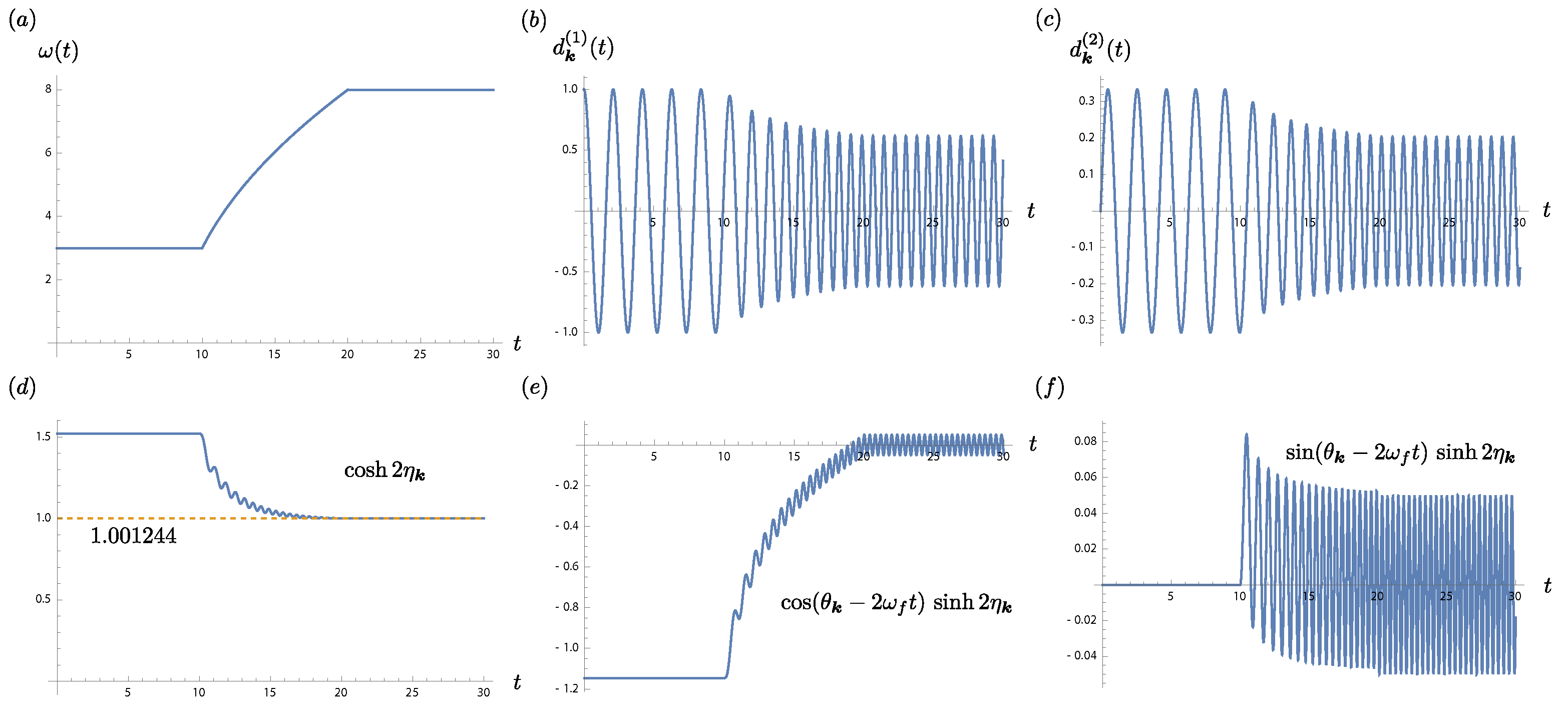
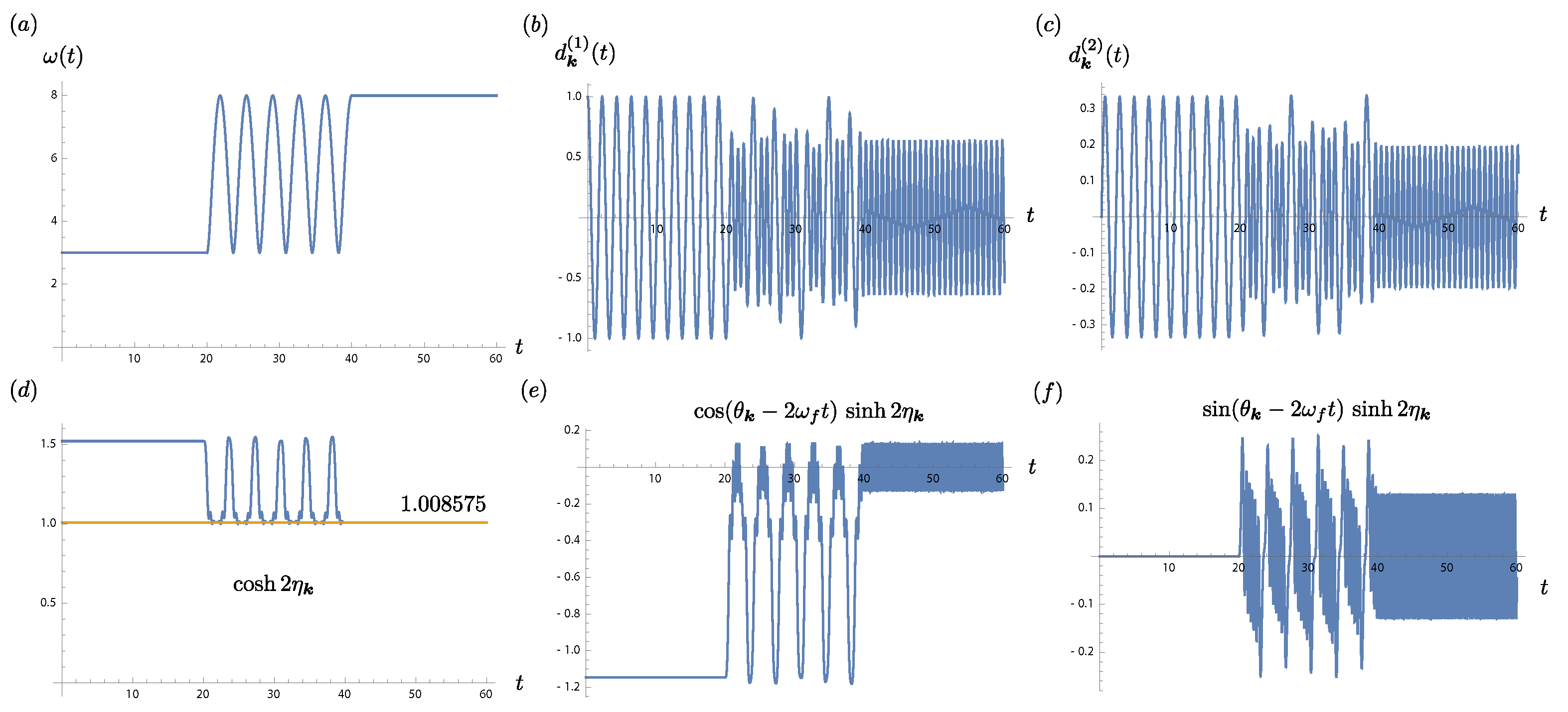
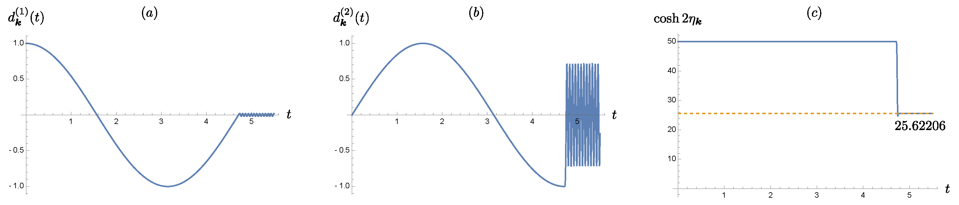
5. Functional Dependence of the Squeeze Parameter on the Parametric Process

Now we turn to how one may possibly extract from the behavior of the squeeze parameter the information of the parametric process that occurs earlier. To be specific, consider the simple case that a massless quantum Klein–Gordon field in flat spacetime undergoes a parametric process such that the frequency of mode k transits smoothly from one constant value ω i for 0 t t a to another constant ω f for t t b > t a .
We would first like to show that the quantum field in the out-region behaves as if it is in its squeezed thermal state with a time-independent squeeze parameter, ζ k , if the initial state of the field at t = 0 is a thermal state. Then, we express the squeeze parameter in terms of the Bogoliubov coefficients, a common tool to treat the dynamics of the quantum field in a parametric (time-varying) process. We also link the squeeze parameter to the fundamental solutions of the equation of motion of the field, in which information of the parametric process is embedded.
We work with the Heisenberg picture, so the field state remains in its initial state at t = 0 . Formally, we can expand the field operator ϕ ^ ( x ) in terms of different sets of mode functions. In the out-region, two convenient choices are
u k IN ( x ) = 1 2 ω i e i k · x d k ( 1 ) ( t ) i ω i d k ( 2 ) ( t ) , u k OUT ( x ) = 1 2 ω f e i k · x e i ω f t ,
where d k ( i ) ( t ) satisfies the equation d ¨ k ( i ) + ω 2 ( t ) d k ( i ) ( t ) = 0 , and u k OUT ( x ) is the standard plane-wave mode function in the out-region, while u k IN ( x ) represents the mode function which evolves from the plane-wave mode function in the in-region. Thus, the field operator may have the expansions,
ϕ ^ ( x ) = k a ^ k u k IN ( x ) + a ^ k u k IN * ( x ) , | k b ^ k u k OUT ( x ) + b ^ k u k OUT * ( x ) , k = d 3 k ( 2 π ) 3 2 ,
in the out-region.
We further suppose that ( b ^ k , b ^ k ) are related to ( a ^ k , a ^ k ) by
b ^ + k = α + k a ^ + k + β k * a ^ k ,
whence the completeness condition | α k | 2 | β k | 2 = 1 implies that the Bogoliubov coefficients, α k and β k , can be parametrized by
α k = cosh η k ,       β k * = e i θ k sinh η k ,
such that
b ^ + k = cosh η k a ^ + k e i θ k sinh η k a ^ k = S ^ 2 ( ζ k ) a ^ + k S ^ 2 ( ζ k ) .
The parametrization (60) can be alternatively implemented by the two-mode squeeze operator S ^ 2 ( ζ k ) . We summarize its properties in Appendix A.
Then, a quantity of the field similar to the Hadamard function in the out-region can be cast into
1 2 IN | ϕ ^ ( x ) , ϕ ^ ( x ) | IN = k 1 2 ω f 1 2 IN | b ^ k , b ^ k | IN e i k · ( x + x ) e i ω f ( t + t ) + 1 2 IN | b ^ k , b ^ k | IN e i k · ( x x ) e i ω f ( t + t ) + 1 2 IN | b ^ k , b ^ k | IN e i k · ( x x ) e i ω f ( t t ) + 1 2 IN | b ^ k , b ^ k | IN e i k · ( x + x ) e i ω f ( t t ) + C . C . = k 1 2 ω f e i k · ( x x ) 1 2 ζ k , IN TMSQ | a ^ k , a ^ k | ζ k , IN TMSQ e i ω f ( t + t ) + 1 2 ζ k , IN TMSQ | a ^ k , a ^ k | ζ k , IN TMSQ e i ω f ( t t ) + C . C . ,
where | ζ k , IN TMSQ = S ^ 2 ( ζ k ) | IN is the two-mode squeezed state of the initial in-state | IN . Thus, Equation (62) gives a Hadamard function in the two-mode squeezed in-state. Although here we use the pure state form, the result can be easily adapted for a mixed state.
On the other hand, the same Hadamard function can be expressed in terms of the in-mode functions, by the expansion
1 2 IN | ϕ ^ ( x ) , ϕ ^ ( x ) | IN = k 1 2 ω i e i k · ( x x ) N k ( β ) + 1 2 d k ( 1 ) ( t ) i ω i d k ( 2 ) ( t ) d k ( 1 ) ( t ) + i ω i d k ( 2 ) ( t ) + C . C . .
If the in-state is a thermal state, then IN | a ^ k , a ^ k | IN is understood in terms of the trace average, and gives 2 N k ( β ) + 1 , with N k ( β ) being the average number density of the thermal state at temperature, β 1 ,
N k ( β ) = 1 e β ω i 1 .
Observe the structural similarities between Equations (62) and (63).
To make them more revealing, we evaluate the expectation values on the right hand side of Equation (62),
IN | b ^ + k , b ^ + k | IN = 0 , IN | b ^ + k , b ^ k | IN = α + k β + k * + α + k β k * 2 N k ( β ) + 1 , IN | b ^ + k , b ^ k | IN = 0 , IN | b ^ + k , b ^ + k | IN = | α + k | 2 + | β k | 2 2 N k ( β ) + 1 .
Thus, Equation (62) becomes
1 2 IN | ϕ ^ ( x ) , ϕ ^ ( x ) | IN = k 1 2 ω f e i k · ( x x ) N k ( β ) + 1 2 2 α k β k * e i ω f ( t + t ) + | α k | 2 + | β k | e i ω f ( t t ) + C . C . .
Comparing this equation with Equation (63), we find that
| α k | 2 + | β k | 2 = 1 2 ω f ω i d k ( 1 ) 2 ( t f ) + ω f ω i d k ( 2 ) 2 ( t f ) + 1 ω f ω i d ˙ k ( 1 ) 2 ( t f ) + ω i ω f d ˙ k ( 2 ) 2 ( t f ) ,
2 α k β k * = 1 2 ω i ω f + i ω f d k ( 1 ) ( t f ) + ω i ω f d k ( 2 ) ( t f ) d ˙ k ( 1 ) ( t f ) + i ω i d ˙ k ( 2 ) ( t f ) × i ω f d k ( 1 ) ( t f ) + ω i ω f d k ( 2 ) ( t f ) + d ˙ k ( 1 ) ( t f ) + i ω i d ˙ k ( 2 ) ( t f ) .
These results easily enable us to find the Bogoliubov coefficients α k and β k once we have the fundamental solutions d k ( i ) ( t ) with i = 1 , 2.
Following the same arguments leading to Equations (62) and (63), if we compute ϕ ^ 2 ( x ) , π ^ 2 ( x ) and ϕ ^ ( x ) , π ^ ( x ) in the out-region, one obtains that, for each mode,
    cosh 2 η k = 1 2 1 ω f ω i d ˙ k ( 1 ) 2 ( t ) + ω i ω f d ˙ k ( 2 ) 2 ( t ) + ω f ω i d k ( 1 ) 2 ( t ) + ω f ω i d k ( 2 ) 2 ( t ) ,
cos ( θ k 2 ω f t ) sinh 2 η k = 1 2 1 ω f ω i d ˙ k ( 1 ) 2 ( t ) + ω i ω f d ˙ k ( 2 ) 2 ( t ) ω f ω i d k ( 1 ) 2 ( t ) ω f ω i d k ( 2 ) 2 ( t ) ,
sin ( θ k 2 ω f t ) sinh 2 η k = 1 ω i d k ( 1 ) ( t ) d ˙ k ( 1 ) ( t ) + ω i d k ( 2 ) ( t ) d ˙ k ( 2 ) ( t ) ,
explicit relations occur between the squeeze parameters and the fundamental solutions. Here, π ^ ( x ) is the canonical momentum conjugated to ϕ ^ ( x ) . Equations (68)–(70) tell us how squeezing may dynamically arise from the parametric process of the field.
As a consistency check, we substitute the coefficients α k and β k on the right hand side by Equation (59), and obtain:
| α k | 2 + | β k | 2 = cosh 2 η k ,       2 α k β k * = e i θ k sinh 2 η k .
Actually, Equations (66) and (67) only determine α k , β k up to a phase factor or a rotation, which we have been ignoring. For example, from (67), we may let
α k = 1 2 ω i ω f + i ω f d k ( 1 ) ( t f ) + ω i ω f d k ( 2 ) ( t f ) d ˙ k ( 1 ) ( t f ) + i ω i d ˙ k ( 2 ) ( t f ) ,
β k = 1 2 ω i ω f i ω f d k ( 1 ) ( t f ) + ω i ω f d k ( 2 ) ( t f ) + d ˙ k ( 1 ) ( t f ) + i ω i d ˙ k ( 2 ) ( t f ) ,
and then we can directly show that Equation (66) is recovered and that
| α k | 2 | β k | 2 = d k ( 1 ) ( t f ) d ˙ k ( 2 ) ( t f ) d ˙ k ( 1 ) ( t f ) d k ( 2 ) ( t f ) = 1 .
However, in this case α k is not real, as Equation (60) implies.
We may recover the missing phase by returning back the rotation operator that we have ignored all along. To be more specific, for example, let the rotation operator R ^ be given by
R ^ ( Φ i ) = exp i Φ i a ^ i a ^ i + 1 2 .
We find R ^ ( Φ i ) a ^ 1 R ^ ( Φ 1 ) = a ^ 1 e i Φ 1 . Then, depending on the order of the rotation operator and the squeeze operator, we may have either
S ^ 2 ( ζ ) R ^ ( Φ i ) a ^ 1 R ^ ( Φ i ) S ^ 2 ( ζ ) = e i Φ 1 cosh η a ^ 1 e i Φ 1 e i θ sinh η a ^ 2 ,
or
R ^ ( Φ i ) S ^ 2 ( ζ ) a ^ 1 S ^ 2 ( ζ ) R ^ ( Φ i ) = e i Φ 1 cosh η a ^ 1 e i Φ 2 e i θ sinh η a ^ 2 .
One can see that there is always a phase ambiguity. In both cases, from Equations (60) and (61), one finds that α k will be complex in general, but actually, one may factor out the overall phase factor for each mode to render α k real.
Before we proceed further with our analysis, let us examine a few illustrative examples.

5.1. Case 1

Consider the parametric process, in which the squared frequency ω 2 ( t ) varies with time according to
ω 2 ( t ) = ω i 2 , 0 t t a , ω i 2 + ω f 2 ω i 2 t t a t b t a , t a t t b , ω f 2 , t t b ,
That is, ω 2 ( t ) is a piecewise-continuous function of time. The time evolution of d k ( 1 ) ( t ) , d k ( 2 ) ( t ) are shown in Figure 2b,c, where one observes that the oscillation amplitudes of the two fundamental solutions change by different amounts, implying the occurrence of quantum squeezing. Notice in Figure 2d that, as t t b the squeeze parameter η k becomes a constant, squeezing is quite small because cosh 2 η k 1 . This small squeezing results from the slow transition rate in the parametric process. The plots Figure 2e,f show oscillations of frequency 2 ω f , consistent with expectation. However, from these plots it is hard to tell whether θ k is time-independent. We take another approach to show it in this section.

5.2. Case 2

In the second example, we choose a nonmonotonic parametric process,
ω 2 ( t ) = ω i 2 , 0 t t a , ω i 2 + ω f 2 ω i 2 sin 2 t t a t b t a n π 2 , t a t t b , ω f 2 , t t b .
Here, n, an odd integer, gives the number of oscillations of the transition process; thus, the frequency variation is not monotonic. The corresponding plots are shown in Figure 3. Since both processes, though continuous, are not smooth, it allows us to see when the transitions start and end. Compared with case 1, the nonmonotonic transition introduces tumultuous behavior in the fundamental solutions d k ( i ) during the transition, in Figure 3b,c, but right after t = t b , the out mode immediately oscillates at frequency ω f . Again, one can see the time-independence of η k in the out-region.
For the simple case we consider here, let us carry out some analysis about the time dependence of the squeeze parameter in the out-region. We may write d k ( i ) ( t ) for t t b as
d k ( 1 ) ( t ) = d k ( 1 ) ( t b ) cos ω f ( t t b ) + d k ( 2 ) ( t b ) 1 ω f sin ω f ( t t b ) ,
d k ( 2 ) ( t ) = d k ( 1 ) ( t b ) 1 ω f sin ω f ( t t b ) + d k ( 2 ) ( t b ) cos ω f ( t t b ) .
The amplitudes of d k ( i ) ( t ) in the out-region are determined by
d k ( 1 ) ( t ) : d k ( 1 ) 2 ( t b ) + d k ( 2 ) 2 ( t b ) ω f 2 1 2 , and d k ( 2 ) ( t ) : d k ( 1 ) 2 ( t b ) ω f 2 + d k ( 2 ) 2 ( t b ) 1 2 ,
which, in turn, are determined by the values of the fundamental solution at the end of the parametric process. We readily find that d k ( 1 ) ( t ) d ˙ k ( 1 ) ( t ) d ˙ k ( 1 ) ( t ) d k ( 1 ) ( t ) = 1 for all t even for the parametric process via the Wronskian of the differential equation that the mode function satisfies.
According to Equation (67), we can show that
| α k ( t ) | 2 + | β k ( t ) | 2 = | α k ( t b ) | 2 + | β k ( t b ) | 2
for all t t b . Since | α k | 2 + | β k | 2 is proportional to cosh 2 η k , Equation (81) then shows that η k is a time-independent constant for all t t b . On the other hand, with the help of Equations (78) and (79), one finds:
1 ω f ω i d ˙ k ( 1 ) 2 ( t ) + ω i ω f d ˙ k ( 2 ) 2 ( t ) ω f ω i d k ( 1 ) 2 ( t ) ω f ω i d k ( 2 ) 2 ( t ) = A k sin ( 2 ω f t b 2 ω f t ) + B k cos ( 2 ω f t b 2 ω f t ) = A k 2 + B k 2 cos ( ϑ k + 2 ω f t b 2 ω f t ) ,
with
A k = 2 1 ω i d k ( 1 ) ( t b ) d ˙ k ( 1 ) ( t b ) + ω i d k ( 2 ) ( t ) d ˙ k ( 2 ) ( t ) ,
B k = 1 ω f ω i d ˙ k ( 1 ) 2 ( t b ) + ω i ω f d ˙ k ( 2 ) 2 ( t b ) ω f ω i d k ( 1 ) 2 ( t b ) ω f ω i d k ( 2 ) 2 ( t b ) .
and
cos ϑ k = B k A k 2 + B k 2 ,             sin ϑ k = A k A k 2 + B k 2 .
From Equations (69) and (70), we see that A k 2 + B k 2 is proportional to sinh 2 η k , and thus is a time-independent constant. One can immediately identify ϑ k in Equations (82)–(84) to be the same θ k in Equations (68)–(70). Finally, we may note that Equation (82) still looks slightly different from the left hand sides of Equations (68)–(70) in the arguments of the trigonometric functions. It results from the choice of the out mode function in Equation (61). The reason for such a choice is that for an observer in the out-region, he has no reference to identify the origin of time coordinate. In addition, the choice of a fixed time origin at most amounts to an absolute phase, which in most cases is of no significance. However, in the current case we are comparing two formalisms; thus, for consistency’s sake, we may define the origin of the time coordinate in the out-region at t b rather than 0. By only shifting t in Equation (61) to t t t b , Equation (82) looks the same as those in Equations (68)–(70). At this point, we have shown that in the out-region an observer may report on having experienced a quantum field in a squeezed thermal state, with a time-independent squeeze parameter.
The squeeze parameter, η k , we showed earlier is quite small because cosh 2 η k 1 . This results from the fact that the parametric processes in the previous cases vary mildly. Now we show a case similar to that in Figure 3 but with a much sharper transition with ω i = 1 , ω f = 100 , t a = 3 π / 2 , t b = 3 π / 2 + 0.05 and n = 1 . The plot for cosh 2 η k is shown in Figure 4. We see in this case that cosh 2 η k = 25.62206 in the out-region, much larger than the previous two cases. Therefore, it is consistent with the understanding that to generate large squeezing, the parametric process had better not be adiabatic. This is corroborated by our prior knowledge of cosmological particle production.
Finally, as a contrast to the previous piecewise-continuous parametric processes, we consider a sufficiently smooth ω 2 ( t ) , such as the thrice-differentiable function ω 2 ( t )
ω 2 ( t ) = ( t t a ) 4 ( t b t a ) 7 20 t 3 10 ( 7 t b 2 t a 2 ) t 2 + 4 ( 21 t b 2 7 t b 2 t a 2 + t a 2 ) t ( 35 t b 3 21 t b 2 t a 2 + 7 t b 2 t a 2 t a 3 ) ,
between t = t a and t = t b . The corresponding results are shown in Figure 5. We do not discern any difference in the generic behavior, so for the quantities of interest in our present study, the piecewise-continuous ω 2 ( t ) suffices.
The fact that the squeeze parameter becomes time-independent in the out-region implies that this result is time-translation-invariant. To be more precise, if we shift the parametric process along the time axis, then as long as the conditions that (1) the observation time t is still in the out-region of the shifted process and (2) the initial time t i remains in the in-region of the shifted process are satisfied, the observer at time t will still see the same squeeze parameter. In other words, the observer in the out-region cannot extract from the squeeze parameter any information about when the parametric process starts or ends. At first, it sounds odd that there exists such a time-translation invariance for a nonequilibrium, nonstationary process. We show this in Appendix D; however, after seeing these examples, this result may not appear that dubious. The full evolution from the initial time t i to the observation time t is not invariant under time translation, but after the parametric process has ended at t b , the mode functions in the out-region reverts to a sinusoidal time dependence. The time translation in a sinusoidal function of time amounts to a phase shift. Thus, if the quantity of interest is independent of this phase shift, it appears to possess time-translation invariance.
Although in the current configuration the detector in the out-region will sense the same squeeze parameter when the parametric process is shifted along the time axis, the measured results in the detector still depend on the duration t b t a and the functional form of the process. Actually, this can be expected from Equations (68)–(70), where the squeeze parameters are expressed in terms of the fundamental solutions, which in turn depend on the functional form of the parametric process in their equation of motion.
For illustration, Figure 6a shows the dependence of the squeeze parameter, η k , on the duration of the parametric process, given by Equation (76). We fix the starting time, t a , of the parametric process and the moment t the measurement in the out-region is performed. We find that the squeeze parameter η k , defined in Equation (68), is oscillatory but decreases with increasing ending time, t b . Except for the small oscillations, the curve in Figure 6a gives the general trend that the squeezing (as manifested, e.g., in particle pair production), is subdued with a slower transition rate or longer transition duration t b t a . This example shows that this kind of parametric process gives a lower production of particles as it moves toward the adiabatic regime. The mild oscillations may be related to the kinks at t a and t b due to the nonsmoothness of ω ( t ) . This may be seen from the observation that the oscillations, as shown in the blow-ups in Figure 6a, appear shallower with larger t b t a because the kinks are less abrupt. This argument also find its support from Figure 7b,d.
In Figure 7, the dependence of the squeeze parameter η k on the functional form of the parametric process is shown. We choose three different parametric processes of ω 2 ( t ) for examples. In Figure 7a, the process has the piecewise-continuous form given by Equation (76), so it gives the same result as Figure 6a. Figure 7b is described by the smooth transition, Equation (86). We have the same process, Equation (77), for Figure 7c,d, but with different choices of n. We choose n = 11 for Figure 7c and n = 1 for Figure 7d. Thus, in Figure 7c, the transition does not monotonically vary with time.
Since both Figure 7b,d are associated with smooth parametric processes, when we prolong the duration of the parametric processes by fixing t a and increasing t b , we see that the value of η k monotonically decreases without any ripples. Thus, together with the behavior of the curve in Figure 6a, they imply that the ripples in Figure 7a may originate from the nonsmoothness of the parametric process at the transition times t a and t b .
Among the plots in Figure 7, Figure 7c shows a more interesting behavior. The transition described by Equation (77) with n = 11 is sinusoidal, as shown in Figure 3a. The squeeze parameter η k in Figure 7c then reveals more structures, and may signify the presence of resonance, shown by a large peak. It seems to imply that the particle production can be greatly enhanced if the transition duration is tuned to the right value for fixed ω i and ω f , as in parametric resonance. This may constitute a mechanism to generate stronger squeezing, in addition to the common one in a runaway setting [23,24]. Another unusual feature is that η k in Figure 7c is not significantly reduced when we have a larger t b .
Actually, this resonance feature can be traced back to parametric instability. We write the equation of motion for a parametric oscillator with the frequency given by Equation (77) into the canonical form
x ( τ ) + a 2 q cos ( 2 τ ) x ( τ ) = 0 ,
where a prime represents taking the derivative with respect to τ , Ω t = 2 τ , and
a = 4 A 2 Ω 2 , q = 2 B 2 Ω 2 , Ω = n π t b t a , A 2 = ω f 2 + ω i 2 2 , B 2 = ω f 2 ω i 2 2 .
Now, comparing the stability diagram Figure 8a of Equation (87) with Figure 7c, one immediately notices that the portion of the curve in Figure 8b that corresponds to exceptionally high squeezing is essentially located within the unstable region (white area) of the stability diagram in Figure 8a. Thus, the large squeezing in the mode driven by a nonmonotonic ω ( t ) is caused by instability in parametric resonance.
The above examples illustrate a point that the dependence of the squeeze parameter η k on the duration of the parametric process does reflect qualitative features of the parametric process. Actually, we can apply the same idea to the spectral dependence of the squeeze parameter for various functional forms of the parametric processes. These will serve as templates from which we may extract qualitative information about the parametric process that the quantum field has experienced.

6. Summary

A major task of theoretical cosmology is to find ways to deduce the state of the early universe from relics observed today such as features of primordial radiation and matter contents. In addition to particle creation at the Planck time and structure formation after the GUT (grand unified theory) time, we add here another fundamental quantum process: quantum radiation from atoms induced by of quantum fields.
A massless quantum field in Minkowski space is subjected to a parametric process which varies the frequencies of the normal modes of the field from one constant value to another over a finite time interval. The initial (in-) state of the field will become squeezed after the process. In the out-region we couple an atom to this field in the out-state; the response of the atom certainly depends on this squeezing. Meanwhile, the radiation generated by the interacting atom will send out signals outwards, such that an observer or a probe at a much later time may still be able to identify the squeezing via the signatures in the radiation.
Once we have identified the squeezing, locally or remotely, we then ask how the squeezing may depend on the details of the parametric process the field had been subjected to. If we can work out templates that relate these quantities, then measurements of certain features of squeezing can tell us something about the parametric process.
The salient points in our results are summarized below. In the first part of this paper we showed the following:
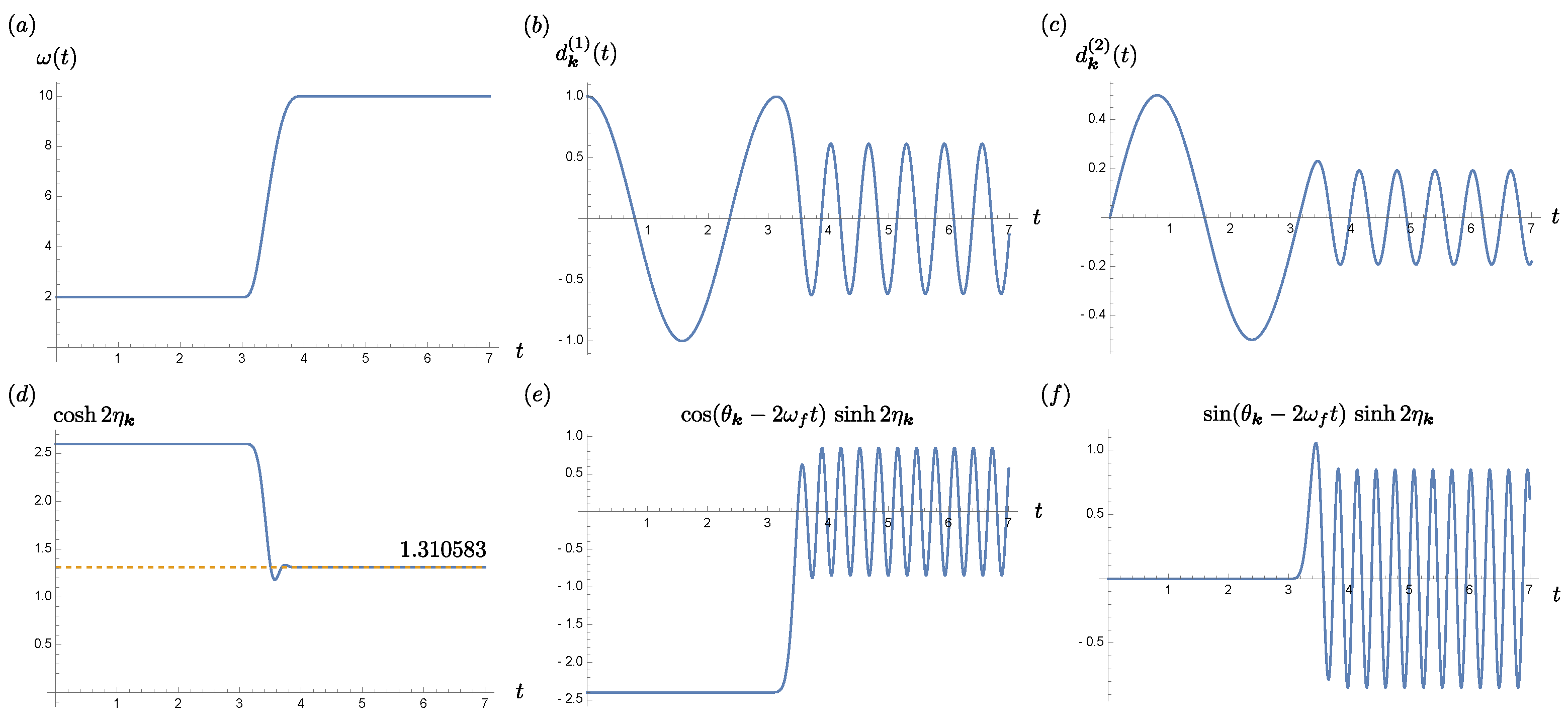
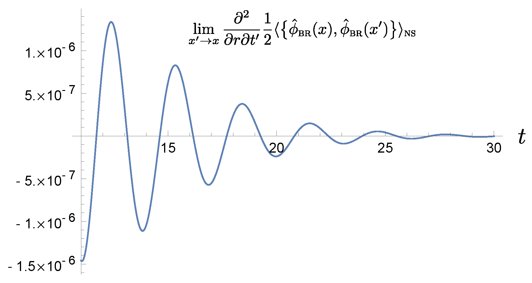
  • The radiation field at a location far away from the atom looks stationary; its nonstationary component decays with time exponentially fast.
  • The net energy flow cancels at late times, similar to the case discussed in Ref. [2]. These features are of particular interest considering that the atom that emits this radiation is coupled to a squeezed field, which is nonstationary by nature. However, they are consistent with the fact that the atom’s internal dynamics relaxes in time.
  • This implies that we are unable to measure the extent of squeezing by measuring the net radiation energy flow at a location far away from the atom.
  • On the other hand, one can receive residual radiation energy density at late times, which is a time-independent constant and is related to the squeeze parameter. However, it is of a near-field nature, so the observer cannot be located too far away from the atom.
Note that there is always an ambient free component of the same squeezed quantum field everywhere, in addition to the above radiation component generated by the atom’s internal motion.
In the second part of this paper we focused on the dependence of the squeeze parameter on the parametric process and obtained these results:
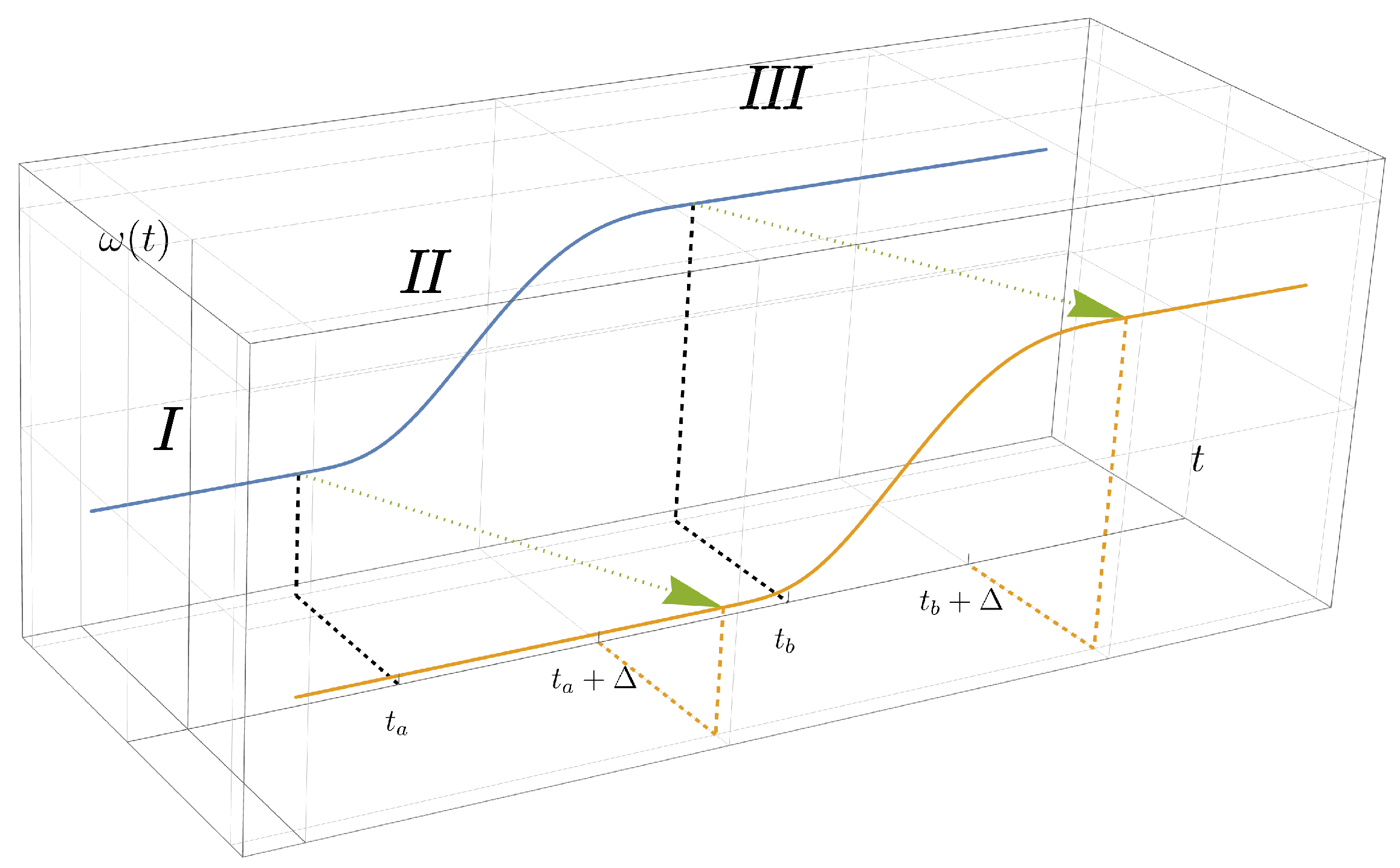
  • Formally it can be shown that the squeeze parameter depends on the evolution of the field in the parametric process.
  • In the current configuration, for a given parametric process, the squeeze parameter depends only on the duration of the process; it does not depend on the starting or the ending time of the process.
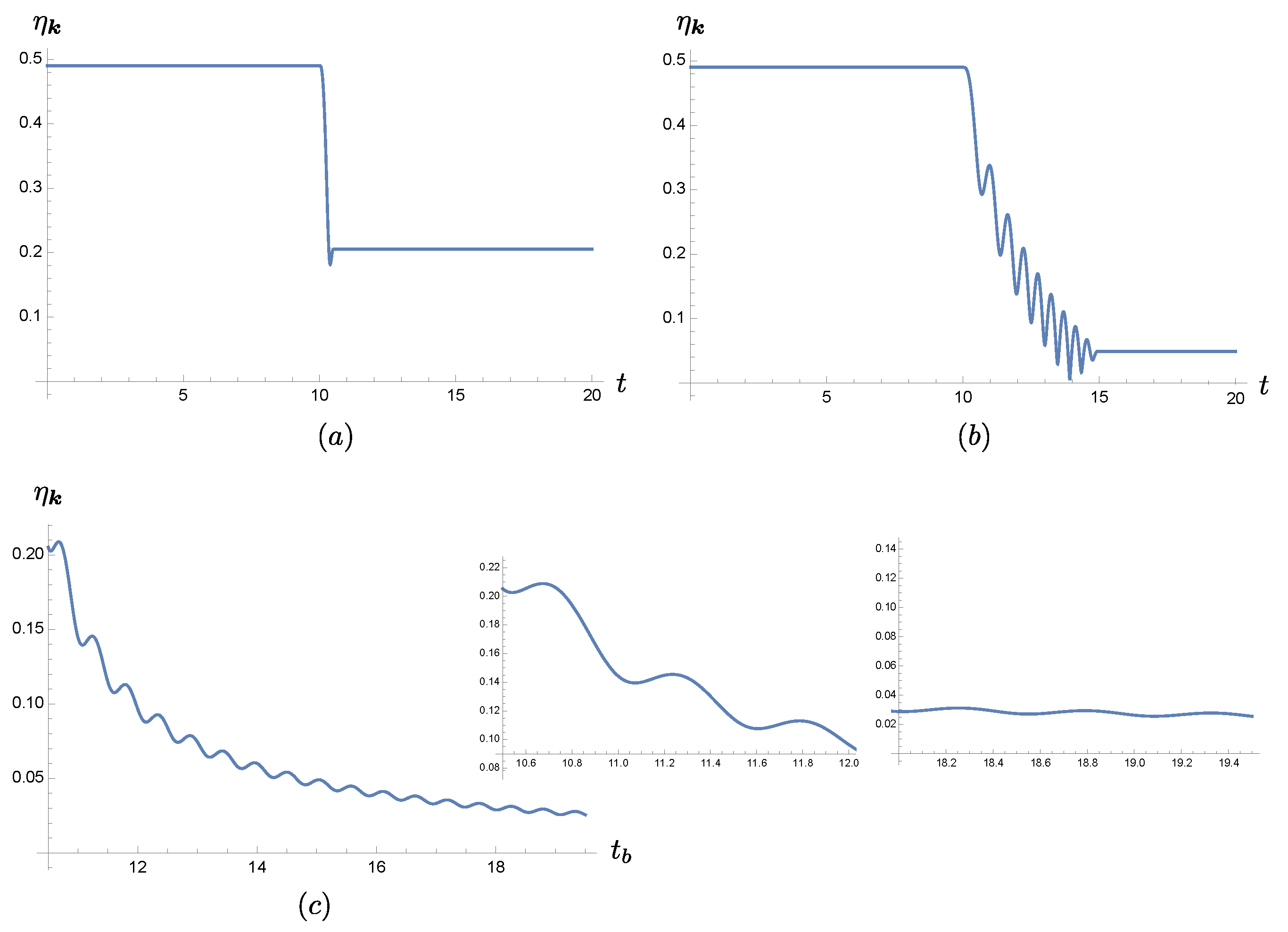
  • In general, for a monotonically varying process, the value of the squeeze parameter decreases with increasing duration of the process.
  • This implies that, for an adiabatic parametric process, the squeezing tends to be quite small, but it can be quite significant for nonadiabatic parametric processes. These results are consistent with studies of cosmological particle creation in the 1970s as parametric amplification of vacuum fluctuations.
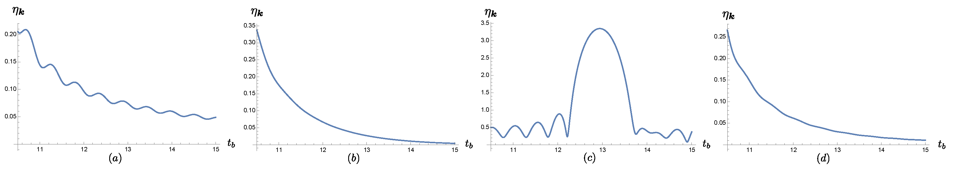
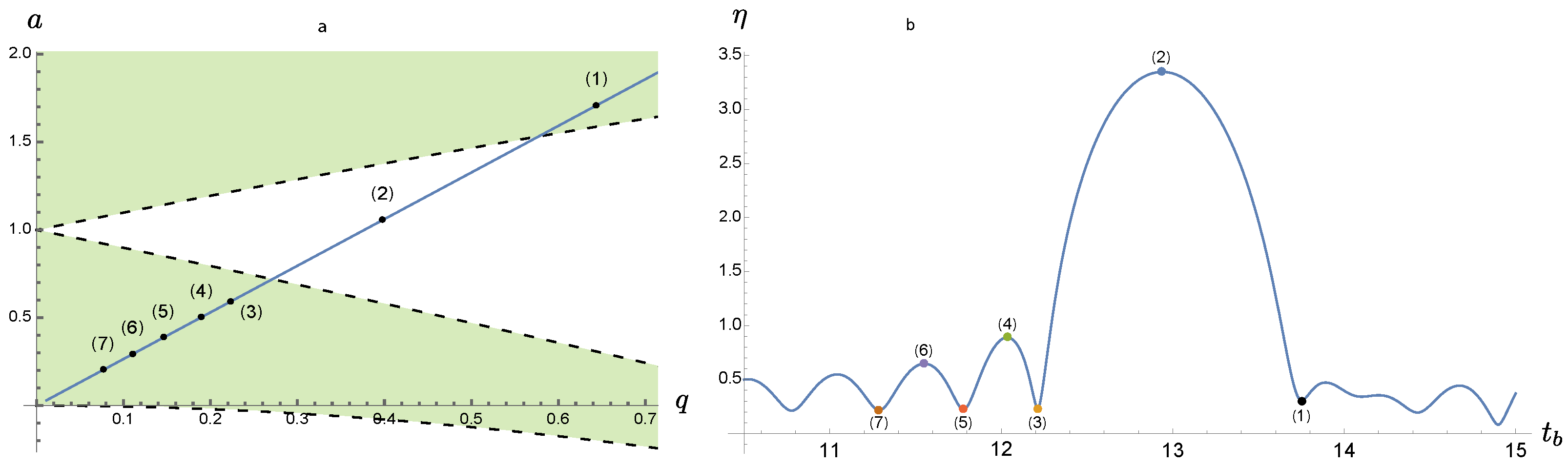
  • If the parametric process changes with time sinusoidally, then the dependence of the squeeze parameter on the duration of the process shows interesting additional structures. For certain lengths of the process, the squeeze parameter can have unusually large values.
  • This nonmonotonic behavior turns out to be related to parametric instability. The resulting large squeeze parameter is caused by the choice of the parameter that falls within the unstable regime of the parametric process.
Our results in this second part indicate that not much information about a monotonic parametric process can be gleaned from the squeeze parameter. On the other hand, for a nonmonotonic parametric process, the squeeze parameter shows nontrivial dependence on the duration of the process. The latter is expected to be the typical case in nature in which various scales are involved in a transition. Moreover, to conform to realistic measurements, we can apply similar considerations to examine the mode dependence of the squeeze parameter. Thus, the current scenario seems to offer a viable means to extract partial information about the parametric process a quantum field has undergone.
As a final remark, we comment on applying the discussions in Section 4 to the case of the atom coupled to quantized electromagnetic fields. To begin with, in conventional sense, such a configuration has supra-Ohmic, Markovian dynamics. It is inherently unstable, as discussed in Ref. [25]. It has runaway solutions, so it makes no sense to discuss the late-time behavior, relaxation, energy balance, or the fluctuation–dissipation relation of such a system. Although we may render such a system to have stable dynamics by resorting to order reduction [26] via the critical manifold argument, this approach is not satisfactory from the viewpoint of open systems because order reduction only asymmetrically changes the behavior of the dissipation on the atom side; it does not accordingly modify the fluctuation noise force on the atom. Thus, the resulting nonequilibrium fluctuation–dissipation relation associated with the atom’s internal dynamics will not take the elegant form we usually see for the Ohmic, Markovian dynamics. Furthermore, this relation will depend on the parameters of the reduced system, and thus loses its universality for interacting linear systems and for some nonlinear systems.
To restore the stable dynamics of the atom’s internal dynamics [25] and the beauty of the associated nonequilibrium fluctuation–dissipation relation, it is probably easier if we generalize the Markovian spectrum of the quantized electromagnetic field to the non-Markovian one. However, this introduces additional complexity to the analysis presented in Section 4 because the radiation field will not have a simple local (apart from retardation) form similar to Equation (47). Thus, it is not clear yet whether the rather general properties we expounded in Section 4 for a quantum scalar field also convey to a quantized electromagnetic field; this is a topic saved for future investigation.

Author Contributions

Conceptualization, J.-T.H. and B.-L.H.; methodology, M.B. and J.-T.H.; formal analysis, M.B. and J.-T.H.; investigation, M.B. and J.-T.H.; writing—original draft preparation, M.B., J.-T.H. and B.-L.H.; writing—review and editing, M.B., J.-T.H. and B.-L.H.; visualization, J.-T.H.; funding acquisition, J.-T.H. All authors have read and agreed to the published version of the manuscript.

Funding

J.-T.H. is supported by the Ministry of Science and Technology of Taiwan, R.O.C., under Grant No. MOST 111-2811-M-008-022.

Data Availability Statement

Not applicable.

Acknowledgments

B.-L.H. appreciates the kind hospitality of Chong-Sun Chu of the National Center for Theoretical Sciences and Hsiang-nan Li of the Academia Sinica in the finishing stage of this paper.

Conflicts of Interest

The authors declare no conflict of interest.

Appendix A. Two-Mode Squeezed State

Here, we outline the properties of the two-mode squeezed operator S ^ 2 ( ζ ) associated mode 1 and 2,
S ^ 2 ( ζ ) = exp ζ * a ^ 1 a ^ 2 ζ a ^ 1 a ^ 2 ,
such that the two-mode squeezed thermal state is defined by
ρ ^ TMST = S ^ 2 ( ζ ) ρ ^ β S ^ 2 ( ζ ) .
where ρ ^ β is a thermal state. The creation and annihilation operators satisfy the standard commutation relation [ a ^ , a ^ ] = 1 . It is convenient to place the squeeze parameter ζ into a polar form ζ = η e i θ , with η R + and 0 θ < 2 π . We thus have
S ^ 2 a ^ 1 S ^ 2 = cosh η a ^ 1 e + i θ sinh η a ^ 2 ,         S ^ 2 a ^ 2 S ^ 2 = cosh η a ^ 2 e + i θ sinh η a ^ 1
such that
a ^ i 2 TMST = Tr ρ β S ^ 2 a ^ i 2 S ^ 2 = 0 ,                                       a ^ i 2 TMST = 0 ,
a ^ 1 a ^ 1 TMST = n ¯ 1 + 1 cosh 2 η + n ¯ 2 sinh 2 η , a ^ 1 a ^ 1 TMST = n ¯ 1 cosh 2 η + n ¯ 2 + 1 sinh 2 η ,
a ^ 2 a ^ 2 TMST = n ¯ 2 + 1 cosh 2 η + n ¯ 1 sinh 2 η , a ^ 2 a 2 TMST = n ¯ 2 cosh 2 η + n ¯ 1 + 1 sinh 2 η ,
a 1 ^ a ^ 2 TMST = e + i ϕ 2 n ¯ 1 + n ¯ 2 + 1 sinh 2 η , a ^ 1 a 2 TMST = e i ϕ 2 n ¯ 1 + n ¯ 2 + 1 sinh 2 η ,
where n ¯ i is the mean particle number of the thermal state associated with mode i,
n ¯ i = Tr ρ ^ β a ^ i a ^ i
It is interesting to compare with the single-mode squeezed thermal state ρ ^ ST , defined by
ρ ^ ST = S ^ ( ζ ) ρ ^ β S ^ ( ζ ) .
Here, S ^ ( ζ ) is the squeezed operator,
S ^ ( ζ ) = exp 1 2 ζ * a ^ 2 1 2 ζ a ^ 2 .
We then find:
a ^ ST = 0 = a ST ,
a ^ 2 ST = e + i θ sinh 2 η n ¯ + 1 2 , a 2 ST = e i θ sinh 2 η n ¯ + 1 2 ,
a ^ a ^ ST = cosh 2 η n ¯ + 1 2 1 2 = cosh 2 η n ¯ + sinh 2 η ,
where n ¯ is the mean particle number of the thermal state. Both the two single-mode squeezed state and the two-squeezed state are connected. We first write two modes in terms of their normal modes i = ± ,
a ^ 1 = a ^ + + a ^ 2 , a ^ 2 = a ^ + a ^ 2 ,
with [ a ^ + , a ^ ] = 0 . Then we can write the two-mode squeeze operator, S ^ 2 in (A1), as
S ^ 2 = exp ζ * 2 a ^ + + a ^ a ^ + a ^ ζ 2 a ^ + + a ^ a ^ + a ^ = exp ζ * 2 a ^ + 2 ζ 2 a ^ + 2 × exp ζ * 2 a ^ 2 + ζ 2 a ^ 2 = S ^ a ^ + ( ζ ) × S ^ a ^ ( ζ ) .
That is, in terms of the normal modes, it can be decomposed into a product of two single-mode squeezed operators.
In the current setting, the connection is even closer because the pair of modes in S ^ 2 have the opposite momenta ± k . Since the two-mode squeeze operator, S ^ 2 in (A1) symmetrically contains the annihilation and the creation operators of both modes, during the mode counting, contributions from each pair ( k , k ) will appear twice, and the resulting expressions may look similar to that given by two single-mode squeezed state. For example, let us compute the Hadamard function of the scalar field ϕ in the two-mode squeezed thermal state in spatially isotropic spacetime,
G H , 0 ( ϕ ) ( x , x ) = d 3 k ( 2 π ) 3 2 1 2 ω d 3 k ( 2 π ) 3 2 1 2 ω 1 2 a ^ k , a ^ k TMST e i k · x + i k · x e i ω t i ω t + 1 2 a ^ k , a ^ k TMST e i k · x i k · x e i ω t + i ω t + H . C . = d 3 k ( 2 π ) 3 1 2 ω 1 2 a ^ k , a ^ k TMST e i k · ( x + x ) e i ω ( t + t ) + 1 2 a ^ k , a ^ k TMST e i k · ( x x ) e i ω ( t + t ) + 1 2 a ^ k , a ^ k TMST e i k · ( x x ) e i ω ( t t ) + 1 2 a ^ k , a ^ k TMST e i k · ( x + x ) e i ω ( t t ) + H . C . = d 3 k ( 2 π ) 3 1 2 ω e i k · ( x x ) n ω + 1 2 cosh 2 η ω e i ω ( t t ) e i θ ω n ω + 1 2 sinh 2 η ω e i ω ( t + t ) + H . C . ,
with ω = | k | and the help of Equations (A4)–(A7). This is the same as the Hadamard function of the field in the squeezed thermal state, consistent with Equation (A15).

Appendix B. Late-Time Behavior of Δ T ^ μ ν

Appendix B.1. Late-Time Energy Flux Density Δ T ^ t r

Here, we examine the late-time net radiation flux of the field at distance r sufficiently far away from the atom, so that only the dominant contribution, independent r, is of our interest. The energy flux density is given by
Δ T ^ r t ( x ) = lim x x 2 r t G H ( ϕ ) ( x , x ) G H , 0 ( ϕ ) ( x , x ) .
Let us first look at the stationary component.

Appendix B.1.1. Stationary Component Δ T ^ t r ST

We assume that t r , but place no other restrictions on r for the moment. Following the decomposition in Equation (24), the stationary part of the contribution purely from the radiation field is given by
lim x x 2 r t 1 2 ϕ ^ BR ( x ) , ϕ ^ BR ( x ) ST = e 2 d ω 2 π ω 2 G ˜ H ( χ ) ( ω ) | G ˜ R , 0 ( ϕ ) ( x ; ω ) | 2 ,
with the help of
r G ˜ R , 0 ( ϕ ) ( x ; ω ) = i ω 1 r G ˜ R , 0 ( ϕ ) ( x ; ω ) ,
r G ˜ H , 0 ( ϕ ) , ST ( x ; ω ) = cosh 2 η coth β ω 2 ω Re G ˜ R , 0 ( ϕ ) ( x ; ω ) 1 r Im G ˜ R , 0 ( ϕ ) ( x ; ω ) ,
where the stationary part of the free-field Hadamard function is
G ˜ H , 0 ( ϕ ) , ST ( x , 0 ; ω ) G ˜ H , 0 ( ϕ ) , ST ( x ; ω ) = cosh 2 η coth β ω 2 sin ω r 4 π r .
To arrive at Equation (A18), we observe that the term proportional to r 1 is odd in ω , thus, vanishing, and that Re G ˜ R ( χ ) ( ω ) is an even function of ω . At time greater than the relaxation time scale we may make the identification
G ˜ H ( χ ) ( ω ) = cosh 2 η coth β ω 2 Im G ˜ R ( χ ) ( ω ) ,
by the nonequilibrium fluctuation–dissipation relation [18,19,22] of the internal dynamics of the atom if it is initially coupled to a squeezed thermal field.
On the other hand, for the cross-term, containing the correlation between the radiation field and the free field at large distance from the atom, its stationary part is
lim x x 2 r t 1 2 ϕ ^ h ( x ) , ϕ ^ BR ( x ) ST + ϕ ^ BR ( x ) , ϕ ^ h ( x ) ST = i e 2 d ω 2 π ω 2 ρ ( ST ) ( ω ) G ˜ R ( χ ) ( ω ) | G ˜ R , 0 ( ϕ ) ( x ; ω ) | 2 .
Hereafter, it is convenient to introduce the shorthand notations
ρ ( ST ) ( ω ) = cosh 2 η coth β ω 2 , and ρ ( NS ) ( ω ) = sinh 2 η coth β ω 2 .
Since the contribution from Re G ˜ R ( χ ) ( ω ) is an even function of ω , one immediately notices that it is the opposite of Equation (A18) by Equation (A22), and thus cancels with Equation (A18). We already know from the case of the unsqueezed thermal state that the corresponding contributions of Equations (A18) and (A23) cancel with one another. Therefore, here, we showed that at late times the stationary part of the net energy flux density far away from the atom vanishes even though the field is initially in the squeezed thermal state, a nonstationary configuration.
Here, it is worth emphasizing the significance of vanishing stationary component of the net radiation flux. This is a unique feature of self-consistent quantum dynamics. The cancellation between Equations (A18) and (A23) is not possible if the radiated field ϕ R ( x ) is not correlated with the free field ϕ h ( x ) . This correlation is established because the atom that sends out the radiation field is driven by a free field, as seen by the Langevin equation (7). It still holds when the field state is a vacuum state [2], so a pure classical system will not have such correlation. Secondly, our system is distinct from the classical driven dipole because the latter has a net outward radiation flux supplied by the external driving agent and is then independent of the field state. This is best seen from the component (A18) of the flux that is solely composed of the radiation field. This flux is field-state-dependent because the internal dynamics of the atom are driven by the quantum fluctuations of the field, rather than an external agent.

Appendix B.1.2. Nonstationary Component Δ T ^ t r NS

Now we turn to the nonstationary contribution in Δ T ^ r t ( x ) . The component purely from the radiation field is given by
lim x x 2 r t 1 2 ϕ ^ BR ( x ) , ϕ ^ BR ( x ) NS = i e 4 0 d ω 2 π ω 2 4 π ρ ( NS ) ( ω ) i ω 1 r G ˜ R ( χ ) ( ω ) G ˜ R , 0 ( ϕ ) ( x ; ω ) 2 e i 2 ω t + i θ + C . C . ,
while the counterpart from the cross-term is
lim x x 2 r t 1 2 ϕ ^ h ( x ) , ϕ ^ BR ( x ) NS + ϕ ^ BR ( x ) , ϕ ^ h ( x ) NS = i e 2 0 d ω 2 π ω ρ ( NS ) ( ω ) G ˜ R ( χ ) ( ω ) G ˜ R , 0 ( ϕ ) ( x ; ω ) ω G ˜ R , 0 ( ϕ ) ( x ; ω ) 2 r Im G ˜ R , 0 ( ϕ ) ( x ; ω ) e i 2 ω t + i θ + C . C . .
Contrary to the stationary contribution, in general, Equation (A25) does not cancel Equation (A26). This can be explicitly shown by examining the sum of the expressions which are proportional to ω inside the curly brackets in both equations. We find that these terms together give
i e 2 0 d ω 2 π ω 2 ρ ( NS ) ( ω ) G ˜ R ( χ ) ( ω ) G ˜ R , 0 ( ϕ ) ( x ; ω ) 2 i e 2 ω 4 π G ˜ R ( χ ) ( ω ) + 1 e i 2 ω t + i θ + C . C . = i e 2 0 d ω 2 π ω 2 ρ ( NS ) ( ω ) Re G ˜ R ( χ ) ( ω ) G ˜ R ( χ ) * ( ω ) G ˜ R ( χ ) * ( ω ) G ˜ R , 0 ( ϕ ) ( x ; ω ) 2 e i 2 ω t + i θ + C . C . ,
where we use the fact that e 2 = 8 π γ m and
Im G ˜ R ( χ ) ( ω ) = 2 m γ ω | G ˜ R ( χ ) ( ω ) | 2 .
Apparently, Equation (A27) does not vanish in general. If the squeeze angle θ is really a mode- and time-independent constant, we may set θ = 0 without loss of generality and further simplify the nonstationary contribution (A27), in Δ T ^ r t ( x ) to
i e 2 0 d ω 2 π ω 2 ρ ( NS ) ( ω ) G ˜ R , 0 ( ϕ ) ( x ; ω ) 2 G ˜ R ( χ ) * ( ω ) G ˜ R ( χ ) * ( ω ) Re G ˜ R ( χ ) ( ω ) e i 2 ω t .
Equation (A27), or the special case Equation (A29), in general, is time-dependent and is not identically zero.
For completeness, let us write down the sum of the terms proportional to 1 / r in the square brackets in Equations (A25) and (A26), which is
i e 2 r 0 d ω 2 π ω ρ ( NS ) ( ω ) G ˜ R ( χ ) ( ω ) G ˜ R , 0 ( ϕ ) ( x ; ω ) e 2 ω 4 π G ˜ R ( χ ) ( ω ) G ˜ R , 0 ( ϕ ) ( x ; ω ) + 2 Im G ˜ R , 0 ( ϕ ) ( x ; ω ) e i 2 ω t + i θ = e 2 r 0 d ω 2 π ω ρ ( NS ) ( ω ) G ˜ R , 0 ( ϕ ) ( x ; ω ) 2 G ˜ R ( χ ) * ( ω ) G ˜ R ( χ ) * ( ω ) Re G ˜ R ( χ ) ( ω ) + G ˜ R ( χ ) ( ω ) | G ˜ R , 0 ( ϕ ) ( x ; ω ) | 2 e i 2 ω t + i θ ,
plus its complex conjugate. Here, again, we used Equation (A28) to recast the expression into a more compact form. This will be useful later to check the consistency via the continuity equation.
The sum of Equations (A25) and (A26) gives the only contribution of the net radiation flux that is likely to survive after the relaxation time scale. However, in Appendix C, we can argue that although Equations (A25) and (A26) do not cancel in general, their sum still decays with time and, furthermore, it actually falls off to zero exponentially fast, proportional to e 2 γ t .
Thus, combining the discussions about the stationary component, we show that at late times no net radiation flux exudes to spatial infinity from a static atom even though the internal degree of freedom of the atom is driven by the quantum fluctuations of the squeezed field caused by its parametric process. At late times it leaves no trace of detectable signal to a detector at distance much greater than the typical scales in the atom’s internal dynamics, except for the case of extremely large squeezing where we might have the chance to see a trace of the net flux since it will take a longer time to decay. However, the information of the squeeze parameter η can still be read out from the asymptotic equilibrium state of the atom’s internal dynamics.

Appendix B.2. Late-Time Field Energy Density Δ T ^ t t

The energy density is given by
Δ T ^ t t ( x ) = lim x x 1 2 2 t t + 2 r r G H ( ϕ ) ( x , x ) G H , 0 ( ϕ ) ( x , x ) .
That is, we subtract off the energy density of the free field in the squeezed state, and Equation (A31) tells us the change in energy density due to the atom–field interaction.

Appendix B.2.1. Stationary Component Δ T ^ t t ST

We first consider the stationary component of Equation (A31). Following the decomposition (24), the part purely caused by the radiation field is given by
lim x x 1 2 2 t t + 2 r r 1 2 ϕ ^ BR ( x ) , ϕ ^ BR ( x ) ST = e 2 d ω 2 π ρ ( ST ) ( ω ) ω 2 + 1 2 r 2 Im G ˜ R ( χ ) ( ω ) | G ˜ R , 0 ( ϕ ) ( x ; ω ) | 2 .
The contribution from the cross-term is then
lim x x 1 2 2 t t + 2 r r 1 2 ϕ ^ h ( x ) , ϕ ^ BR ( x ) ST + ϕ ^ BR ( x ) , ϕ ^ h ( x ) ST = e 2 d ω 2 π ρ ( ST ) ( ω ) ω 2 + 1 2 r 2 | G ˜ R , 0 ( ϕ ) ( x ; ω ) | 2 Im G ˜ R ( χ ) ( ω ) + ω r Re G ˜ R ( χ ) ( ω ) G ˜ R , 0 ( ϕ ) 2 ( x ; ω ) 1 2 r 2 Im G ˜ R ( χ ) ( ω ) G ˜ R , 0 ( ϕ ) 2 ( x ; ω ) ,
with the help of Equations (A19) and (A20) to re-express the term
2 Re G ˜ R ( χ ) ( ω ) G ˜ R , 0 ( ϕ ) ( x ; ω ) Im G ˜ R , 0 ( ϕ ) ( x ; ω ) = | G ˜ R , 0 ( ϕ ) ( x ; ω ) | 2 Im G ˜ R ( χ ) ( ω ) + Im G ˜ R ( χ ) ( ω ) G ˜ R , 0 ( ϕ ) 2 ( x ; ω ) .
Adding both contributions together gives
Δ T ^ t t ST = e 2 d ω 2 π ρ ( ST ) ( ω ) ω r Re G ˜ R ( χ ) ( ω ) G ˜ R , 0 ( ϕ ) 2 ( x ; ω ) 1 2 r 2 Im G ˜ R ( χ ) ( ω ) G ˜ R , 0 ( ϕ ) 2 ( x ; ω ) ,
at late times and at large distance away from the atom. The dominant contribution of the stationary component of the local field energy density vanishes, so Equation (A34) is subdominant since it is proportional to 1 / r 3 . It comes from the correlation between the radiation field and the free field at the location far away from the atom, and it decays faster with r. Note that there are two type of 1 / r 3 contributions in the cross-terms (A33) but one of them cancels with its counterpart in Equation (A32). The residual energy density (A34) has a relatively short range by nature. We note that it is proportional to e 2 , which is proportional to the damping constant, γ . Since this is a time-independent constant, it means that this may be an unambiguous aftereffect of the transient peregrinating radiation field.
Next, we turn to the nonstationary component.

Appendix B.2.2. Nonstationary Component Δ T ^ t t NS

We first examine the late-time contribution purely from the radiation field,
lim x x 1 2 2 t t + 2 r r 1 2 ϕ ^ BR ( x ) , ϕ ^ BR ( x ) NS = e 4 0 d ω 2 π ω 4 π ρ ( NS ) ( ω ) ω 2 + i ω r 1 2 r 2 G ˜ R ( χ ) ( ω ) G ˜ R , 0 ( ϕ ) ( x ; ω ) 2 e i 2 ω t + i θ + C . C . .
On the other hand, the corresponding contribution from the cross-term gives
lim x x 1 2 2 t t + 2 r r 1 2 ϕ ^ h ( x ) , ϕ ^ BR ( x ) NS + ϕ ^ BR ( x ) , ϕ ^ h ( x ) NS = e 2 0 d ω 2 π ρ ( NS ) ( ω ) i ω 2 + i ω r G ˜ R ( χ ) ( ω ) G ˜ R , 0 ( ϕ ) ( x ; ω ) 2 + 1 r 2 G ˜ R ( χ ) ( ω ) G ˜ R , 0 ( ϕ ) ( x ; ω ) Im G ˜ R , 0 ( ϕ ) ( x ; ω ) e i 2 ω t + i θ + C . C . ,
Now we use the same trick (A28) to combine both contributions, and we obtain:
Δ T ^ t t NS = i e 2 0 d ω 2 π ρ ( NS ) ( ω ) i ω 2 + i ω r 1 2 r 2 G ˜ R , 0 ( ϕ ) ( x ; ω ) 2 G ˜ R ( χ ) * ( ω ) G ˜ R ( χ ) * ( ω ) Re G ˜ R ( χ ) ( ω ) + 1 2 r 2 G ˜ R ( χ ) ( ω ) | G ˜ R , 0 ( ϕ ) ( x ; ω ) | 2 } e i 2 ω t + i θ + C . C . .
The dominant term in Equation (A37) has the same form as Equation (A27), and thus will vanish at late times at distance far away from the atom.
Therefore, at late times, Δ T ^ t t settles down to a constant value whose value decays similar to 1 / r 3 away from the atom.

Appendix B.3. Continuity Equation

Here, in passing, we would like to examine the consistency of our results of the nonstationary components of Δ T ^ μ t in terms of the continuity equation μ T μ t = 0 . It turns out convenient to list the previous results for the relevant components
T ^ r t NS ( RR ) = i e 4 0 d ω 2 π ω 2 4 π ρ ( NS ) ( ω ) i ω 1 r G ˜ R ( χ ) ( ω ) G ˜ R , 0 ( ϕ ) ( x ; ω ) 2 e i 2 ω t + i θ + C . C . , T ^ r t NS ( HR ) = i e 2 0 d ω 2 π ω ρ ( NS ) ( ω ) G ˜ R ( χ ) ( ω ) G ˜ R , 0 ( ϕ ) ( x ; ω ) ω G ˜ R , 0 ( ϕ ) ( x ; ω ) 2 r Im G ˜ R , 0 ( ϕ ) ( x ; ω ) e i 2 ω t + i θ + C . C . , T ^ t t NS ( RR ) = e 4 0 d ω 2 π ω 4 π ρ ( NS ) ( ω ) ω 2 + i ω r 1 2 r 2 G ˜ R ( χ ) ( ω ) G ˜ R , 0 ( ϕ ) ( x ; ω ) 2 e i 2 ω t + i θ + C . C . , T ^ t t NS ( HR ) = e 2 0 d ω 2 π ρ ( NS ) ( ω ) G ˜ R ( χ ) ( ω ) i ω 2 + i ω r G ˜ R , 0 ( ϕ ) ( x ; ω ) 2 + 1 r 2 G ˜ R , 0 ( ϕ ) ( x ; ω ) Im G ˜ R , 0 ( ϕ ) ( x ; ω ) e i 2 ω t + i θ + C . C . .
The superscript “ RR ” represents the contributions purely from the radiation field such as Equations (A25) and (A35), while the superscript “ HR ” denotes those from the cross-terms such as Equations (A26), and (A36). For our configuration, we do not have T ϑ t and T φ t where ϑ and φ are, respectively, the polar angle, and azimuthal angle, so, explicitly, the continuity equation can be written in the form
μ T ^ μ t = 0 = t T t t 1 r 2 r r 2 T r t .
Thus, we find:
1 r 2 r r 2 T ^ r t NS ( RR ) = 2 i e 4 0 d ω 2 π ω 2 4 π ρ ( NS ) ( ω ) ω 2 + i ω r 1 2 r 2 G ˜ R ( χ ) ( ω ) G ˜ R , 0 ( ϕ ) ( x ; ω ) 2 e i 2 ω t + i θ + C . C . ,
which is equal to t T ^ t t NS ( RR ) , and
1 r 2 r r 2 T ^ r t NS ( HR ) = 2 e 2 0 d ω 2 π ρ ( NS ) ( ω ) G ˜ R ( χ ) ( ω ) i ω 2 + i ω r G ˜ R , 0 ( ϕ ) ( x ; ω ) 2 + 1 r 2 G ˜ R , 0 ( ϕ ) ( x ; ω ) Im G ˜ R , 0 ( ϕ ) ( x ; ω ) e i 2 ω t + i θ + C . C . .
It is exactly t T ^ t t NS ( HR ) . Thus, the continuity equation is satisfied.

Appendix C. Late-Time Behavior of the Nonstationary Contribution in Δ T ^ r t

It turns out that the nonstationary contribution in Δ T ^ r t ( x ) still decays with time. To begin with, it proves useful to quote the late-time expressions of the energy exchange between the atom and the surrounding field [2,22]. For times greater than the relation time, the nonstationary contribution of the energy flow into the atom from the field has the form,
P ξ ( NS ) ( t ) = i e 2 0 d ω 2 π ω 2 4 π sinh 2 η coth β ω 2 G ˜ R ( χ ) ( ω ) e i 2 ω t + i θ C . C . ,
and the corresponding contribution of the energy flow out of the atom due to friction is
P γ ( NS ) ( t ) = e 4 0 d ω 2 π ω 3 ( 4 π ) 2 sinh 2 η coth β ω 2 G ˜ R ( χ ) ( ω ) 2 e i 2 ω t + i θ + C . C . .
For comparison, let us place the terms proportional to ω inside of the curly brackets of (A26) and (A25) here,
(A26) : i e 2 0 d ω 2 π ω 2 ( 4 π ) 2 r 2 sinh 2 η coth β ω 2 G ˜ R ( χ ) ( ω ) e i 2 ω ( t r ) + i θ C . C . ,
(A25) : e 4 0 d ω 2 π ω 3 ( 4 π ) 3 r 2 sinh 2 η coth β ω 2 G ˜ R ( χ ) ( ω ) 2 e i 2 ω ( t r ) + i θ + C . C . .
One can see correspondence between Equations (A39) and (A41), as well as between Equations (A40) and (A42). For example, the integrand of Equation (A41) is e i 2 ω r 4 π r 2 times the integrand of Equation (A39). The same applies to the pair of Equations (A40)–(A42). For a fix r and at times t r , we may shift or redefine t in Equations (A41) and (A42) by t r t such that the integrals in both equations are essentially proportional to those in Equations (A39) and (A40). We numerically showed in Ref. [19] that Equations (A39) and (A40) vanish as t , so we conclude that the terms proportional to ω inside of the curly brackets of Equations (A25) and (A26) will also vanish at late times. For example, as shown in Figure A1, generated by numerical calculations, the contribution in Equation (A25) actually decays exponentially fast to zero.
Figure A1. The time -dependence of Equation (A25), one of the nonstationary components of the radiation flux. The curve falls off to zero exponentially fast. Here, β 1 = 0 , γ = 0.2 , r = 10 , and ω r = 1 are chosen.
Physics 05 00040 g0a1
For terms that are proportional to 1 / r inside of the curly brackets of Equations (A26) and (A25), we immediately see that if we take the time derivative of Equation (A25), we obtain an expression which is 2 / r times Equation (A42). Likewise, the time derivative of Equation (A26) gives
2 r × i e 2 0 d ω 2 π ω 2 ( 4 π ) 2 r 2 sinh 2 η coth β ω 2 G ˜ R ( χ ) ( ω ) e i 2 ω ( t r ) + i θ e i 2 ω t + i θ C . C . .
Following the previous arguments, for a fixed r, it vanishes in the limit t too. Thus, we have demonstrated that the time derivatives of the terms proportional to 1 / r inside of the curly brackets of Equations (A26) and (A25) vanish, so these terms must be constants for sufficiently large time. On the other hand, these terms are time-dependent and are not sign-definite, so the asymptotic constants must be zero.
Placing these results together, we reach the conclusion that the nonstationary terms of the net radiation flux vanish eventually at large distance away from the atom. However, this does tell us how slowly the nonstationary terms decay. Actually, at least for the zero-temperature limit β , we can carry out the above integrals analytically, and the brute-force calculations show that for fixed r, these integrals give results that decay exponentially fast to zero in a form proportional to sinh 2 η e 2 γ t . Thus, at late times, no net radiation energy flux leaks to the spatial infinity from the atom even though the internal degree of freedom of the atom is coupled to a nonstationary squeezed quantum field.

Appendix D. Time-Translational Invariance of the Squeeze Parameter in the Out-Region

Next we argue that if we shift the parametric process by Δ along the time axis, as shown in Figure A2, then we have
d i ( II ) ( t + Δ , t a + Δ ) = d i ( II ) ( t , t a )
where i = 1 , 2, and d i ( II ) ( t + Δ , t a + Δ ) , in sans serif style, is the fundamental solution in-region II for the shifted case described by the orange curve in Figure A2.
Since the fundamental solutions d i ( II ) ( y , y a ) in-region II for the orange curve satisfy the equation of motion
d ¨ i ( II ) ( y , y a ) + ω 2 ( y ) d i ( II ) ( y , y a ) = 0 ,
with the standard initial conditions given at y a = t a + Δ , while the fundamental solutions d i ( II ) ( y , y a ) in-region II for the blue curve satisfy the equation of motion
d ¨ i ( II ) ( t , t a ) + ω 2 ( t ) d i ( II ) ( t , t a ) = 0 ,
with the standard initial conditions given at t a , one can immediately notice that both cases are related by y = t + Δ , and thus we arrive at Equation (A44), and in particular,
d i ( II ) ( t b + Δ , t a + Δ ) = d i ( II ) ( t b , t a ) .
Here below, we use this result.
Figure A2. The parametric process described by a piecewise continuous function. The transition begins at t a , and ends at t b , region II. Between t i and t a , region I, the frequency ω ( t ) takes on a constant value ω i and is given by another constant ω f after t t b , region III. We consider a shift Δ of the parametric process along the timeline while keeping the functional form, the duration t b t a of the process, and the initial time t i of the motion unchanged. We displace these two cases by a horizontal displacement for discernibility. See text for details.
Physics 05 00040 g0a2
Now we would like to explicitly show that a detector, in the out-region with t > t b + Δ , will find the same squeeze parameter for both cases described in Figure A2, independent of the shift Δ , even if it carries out the measurement at the same time t. Note that in both cases the motion starts at the same t i = 0 . We focus on the moment t = t b + Δ , since afterward, the squeeze parameter is a constant. Before we start, let us first note that d i ( I ) ( t ) is essentially the same as d i ( I ) ( t ) , except that the former applies to the time interval 0 = t i t t a + Δ while the latter only to 0 = t i t t a . With this recognition, we can write d i ( I ) ( t a + Δ ) as
d i ( I ) ( t a + Δ ) = d 1 ( I ) ( Δ ) d i ( I ) ( t a ) + d 2 ( I ) ( Δ ) d ˙ i ( I ) ( t a ) .
Now we write d i ( t b + Δ , 0 ) in terms d i ( x ) with X = I , II, and III of the unshifted process; see Figure A2. We show the calculations explicitly for d 1 ( t b + Δ ) , and the result for d 2 ( t b + Δ ) follows similarly. Pretty straightforwardly, we have:
d 1 ( t b + Δ , 0 ) = d 1 ( II ) ( t b + Δ , t a + Δ ) d 1 ( I ) ( t a + Δ ) + d 2 ( II ) ( t b + Δ , t a + Δ ) d ˙ 1 ( I ) ( t a + Δ ) = d 1 ( II ) ( t b , t a ) d 1 ( I ) ( Δ ) d 1 ( I ) ( t a ) + d 2 ( I ) ( Δ ) d ˙ 1 ( I ) ( t a ) + d 2 ( II ) ( t b , t a ) d ˙ 1 ( I ) ( Δ ) d 1 ( I ) ( t a ) + d ˙ 2 ( I ) ( Δ ) d ˙ 1 ( I ) ( t a )
with the help of Equations (A44) and (A48). We use a trick that only applies to the undamped harmonic oscillator. For in-region I, we have the identities,
d ˙ 2 ( I ) ( t ) = d 1 ( I ) ( t ) , d 2 ( I ) ( Δ ) d ˙ 1 ( I ) ( t a ) = d 2 ( I ) ( t a ) d ˙ 1 ( I ) ( Δ ) ,
and it allows us to rewrite Equation (A49),
d 1 ( t b + Δ , 0 ) = d 1 ( II ) ( t b , t a ) d 1 ( I ) ( Δ ) d 1 ( I ) ( t a ) + d ˙ 1 ( I ) ( Δ ) d 2 ( I ) ( t a ) + d 2 ( II ) ( t b , t a ) d ˙ 1 ( I ) ( Δ ) d 1 ( I ) ( t a ) + d 1 ( I ) ( Δ ) d ˙ 1 ( I ) ( t a ) = d 1 ( II ) ( t b , t a ) d 1 ( I ) ( t a ) + d 2 ( II ) ( t b , t a ) d ˙ 1 ( I ) ( t a ) d 1 ( I ) ( Δ ) + d 1 ( II ) ( t b , t a ) d 2 ( I ) ( t a ) + d 2 ( II ) ( t b , t a ) d 1 ( I ) ( t a ) d ˙ 1 ( I ) ( Δ ) = d 1 ( t b , 0 ) d 1 ( I ) ( Δ ) + d 2 ( t b , 0 ) d ˙ 1 ( I ) ( Δ ) .
Similarly, for d 2 ( t b + Δ , 0 ) , we have
d 2 ( t b + Δ , 0 ) = d 1 ( t b , 0 ) d 2 ( I ) ( Δ ) + d 2 ( t b , 0 ) d ˙ 2 ( I ) ( Δ ) .
Now we plug these results into the expressions in Equations (68)–(70) to find the corresponding squeeze parameter in out-region III,
1 ω f ω i d ˙ k ( 1 ) 2 ( t b + Δ ) + ω i ω f d ˙ k ( 2 ) 2 ( t b + Δ ) + ω f ω i d k ( 1 ) 2 ( t b + Δ ) + ω f ω i d k ( 2 ) 2 ( t b + Δ ) = 1 ω f ω i d ˙ k ( 1 ) 2 ( t b ) + ω i ω f d ˙ k ( 2 ) 2 ( t b ) + ω f ω i d k ( 1 ) 2 ( t b ) + ω f ω i d k ( 2 ) 2 ( t b ) ,
1 ω f ω i d ˙ k ( 1 ) 2 ( t b + Δ ) + ω i ω f d ˙ k ( 2 ) 2 ( t b + Δ ) ω f ω i d k ( 1 ) 2 ( t b + Δ ) ω f ω i d k ( 2 ) 2 ( t b + Δ ) = 1 ω f ω i d ˙ k ( 1 ) 2 ( t b ) + ω i ω f d ˙ k ( 2 ) 2 ( t b ) ω f ω i d k ( 1 ) 2 ( t b ) ω f ω i d k ( 2 ) 2 ( t b ) ,
1 ω i d k ( 1 ) ( t b + Δ ) d ˙ k ( 1 ) ( t b + Δ ) + ω i d k ( 2 ) ( t b + Δ ) d ˙ k ( 2 ) ( t b + Δ ) = 1 ω i d k ( 1 ) ( t b ) d ˙ k ( 1 ) ( t b ) + ω i d k ( 2 ) ( t b ) d ˙ k ( 2 ) ( t b ) ,
due to
d 1 ( I ) ( Δ ) d ˙ 1 ( I ) ( Δ ) = ω i 2 d 2 ( I ) ( Δ ) d ˙ 2 ( I ) ( Δ ) , d 1 ( I ) 2 ( Δ ) + ω i 2 d 2 ( I ) 2 ( Δ ) = 1 , 1 ω i 2 d ˙ 1 ( I ) 2 ( Δ ) + d ˙ 2 ( I ) 2 ( Δ ) = 1 .
The results for the shifted process are the same as those for the unshifted process. Thus, both cases generate the same squeezing at t t b + Δ .

References

  1. Unruh, W.G. Notes on black-hole evaporation. Phys. Rev. D 1976, 14, 870–892. [Google Scholar] [CrossRef]
  2. Hsiang, J.-T.; Hu, B.L. Atom-field interaction: From vacuum fluctuations to quantum radiation and quantum dissipation or radiation reaction. Physics 2019, 1, 430–444. [Google Scholar] [CrossRef]
  3. DeWitt, B.S. Quantum gravity: The new synthesis. In General Relativity: An Einstein Centenary Survey; Hawking, S.W., Israel, W., Eds.; Cambridge University Press: New York, NY, USA, 1979; pp. 680–745. [Google Scholar]
  4. Ackerhalt, J.R.; Knight, P.L.; Eberly, J.H. Radiation reaction and radiative frequency shifts. Phys. Rev. Lett. 1973, 30, 456–460. [Google Scholar] [CrossRef]
  5. Milonni, P.W.; Smith, W.A. Radiation reaction and vacuum fluctuations in spontaneous emission. Phys. Rev. A 1975, 11, 814–824. [Google Scholar] [CrossRef]
  6. Dalibard, J.; Dupont-Roc, J.; Cohen-Tannodji, C. Vacuum fluctuations and radiation reaction: Identification of their respective contributions. J. Phys. France 1982, 43, 1617–1638. [Google Scholar] [CrossRef]
  7. Dalibard, J.; Dupont-Roc, J.; Cohen-Tannodji, C. Dynamics of a small system coupled to a reservoir: Reservoir fluctuations and self-reaction. J. Phys. France 1984, 45, 637–656. [Google Scholar] [CrossRef]
  8. Jackson, J.D. Classical Electrodynamics; John Wiley & Sons, Inc.: New York, NY, USA, 1975; Available online: https://archive.org/details/ClassicalElectrodynamics2nd/page/n5/mode/2up (accessed on 5 May 2023).
  9. Rohrlich, F. Classical Charged Particles: Foundation of Their Theories; Routledge/Taylor & Francis Group: New York, NY, USA, 2019. [Google Scholar] [CrossRef]
  10. Johnson, P.R.; Hu, B.L. Stochastic theory of relativistic particles moving in a quantum field: Scalar Abraham-Lorentz-Dirac-Langevin equation, radiation reaction, and vacuum fluctuations. Phys. Rev. D 2002, 65, 065015. [Google Scholar] [CrossRef]
  11. Johnson, P.R.; Hu, B.L. Unruh effect in a uniformly accelerated charge: From quantum fluctuations to classical radiation. Found. Phys. 2005, 35, 1117–1147. [Google Scholar] [CrossRef]
  12. Hsiang, J.-T.; Hu, B.L. Quantum radiation and dissipation in relation to classical radiation and radiation reaction. Phys. Rev. D 2022, 106, 045002. [Google Scholar] [CrossRef]
  13. Drummond, P.D.; Ficek, Z. Quantum Squeezing; Springer: Berlin/Heidelberg, Germany, 2004. [Google Scholar] [CrossRef]
  14. Grishchuk, L.P.; Sidorov, Y.V. Squeezed quantum states of relic gravitons and primordial density fluctuations. Phys. Rev. D 1990, 42, 3413–3421. [Google Scholar] [CrossRef]
  15. Hu, B.L.; Kang, G.; Matacz, A. Squeezed vacua and the quantum statistics of cosmological particle creation. Int. J. Mod. Phys. A 1994, 9, 991–1007. [Google Scholar] [CrossRef]
  16. Weinberg, S. Cosmology; Oxford University Press: New York, NY, USA, 2008. [Google Scholar]
  17. Hsiang, J.T.; Hu, B.L. NonMarkovianity in cosmology: Memories kept in a quantum field. Ann. Phys. 2021, 434, 168656. [Google Scholar] [CrossRef]
  18. Hsiang, J.T.; Hu, B.L. Fluctuation-dissipation relation for a quantum Brownian oscillator in a parametrically squeezed thermal field. Ann. Phys. 2021, 433, 168594. [Google Scholar] [CrossRef]
  19. Arısoy, O.; Hsiang, J.T.; Hu, B.L. Quantum-parametric-oscillator heat engines in squeezed thermal baths: Foundational theoretical issues. Phys. Rev. E 2022, 105, 014108. [Google Scholar] [CrossRef]
  20. Parker, L. Quantized fields and particle creation in expanding universes. I. Phys. Rev. 1969, 183, 1057–1068. [Google Scholar] [CrossRef]
  21. Zel’dovich, Y.B. Particle production in cosmology. JETP Lett. 1970, 12, 307–311. Available online: http://jetpletters.ru/ps/1734/article_26352.shtml (accessed on 5 March 2023).
  22. Hsiang, J.T.; Chou, C.H.; Subaşı, Y.; Hu, B.L. Quantum thermodynamics from the nonequilibrium dynamics of open systems: Energy, heat capacity, and the third law. Phys. Rev. E 2018, 97, 012135. [Google Scholar] [CrossRef]
  23. Guth, A.H.; Pi, S.-Y. Quantum mechanics of the scalar field in the new inflationary universe. Phys. Rev. D 1985, 32, 1899–1920. [Google Scholar] [CrossRef]
  24. Hsiang, J.T.; Hu, B.L. No intrinsic decoherence of inflationary cosmological perturbations. Universe 2022, 8, 27. [Google Scholar] [CrossRef]
  25. Hsiang, J.T.; Hu, B.L. Non-Markovian Abraham-Lorenz-Dirac equation: Radiation reaction without pathology. Phys. Rev. D 2022, 106, 125108. [Google Scholar] [CrossRef]
  26. Spohn, H. The critical manifold of the Lorentz–Dirac equation. Europhys. Lett. (EPL) 2000, 49, 287–292. [Google Scholar] [CrossRef]
Figure 1. The configuration of the parametric process of the field. The process changes one of the mode frequencies from ω i at time t t a to ω f at t t b . The transition is assumed to happen continuously. The interaction between an atom and the field is turned on at t 0 > t a and radiation is generated by the internal motion of the atom. For a receiver at distance r away from the atom, it will take another time r to meet the radiation. The relaxation time of the atom’s internal motion is of the order of the inverse of the damping constant, γ 1 .
Physics 05 00040 g001
Figure 2. An example of a parametric process described by Equation (76): (a) the time dependence of the frequency ω ; time evolutions of the two fundamental solutions, (b) d k ( 1 ) and (c) d k ( 2 ) , and (df) the time dependence of the squeeze parameters. ω i = 3 , ω f = 8 , t a = 10 , and t b = 20 are chosen.
Physics 05 00040 g002
Figure 3. An example of a parametric process described by Equation (77): (af) same as in Figure 2. ω i = 3 , ω f = 8 , t a = 10 , t b = 20 , and n = 11 are chosen.
Physics 05 00040 g003
Figure 4. An example of a parametric process described by Equation (77): (a), (b), and (c) same as in Figure 3b, c, and d, respectively, but with ω i = 1 , ω f = 100 , t a = 3 π / 2 , t b = 3 π / 2 + 0.05 , and n = 1 .
Physics 05 00040 g004
Figure 5. An example of a parametric process described by Equation (86): (af) same as in Figure 2. with ω i = 2 , ω f = 10 , t a = 3 , and t b = 4 are chosen.
Physics 05 00040 g005
Figure 6. (a) The t b -dependence of the squeeze parameter, η k for the parametric process described by Equation (76) with ω i = 3 , ω f = 8 , t i = 0 , and t a = 10 . A fictitious detector is placed at t = 20 , and t b varies from 10.5 to 19.5. For comparison, the time dependence of η k when (b) t b = 10.5 and (c) t b = 15 are shown. These two cases are highlighted in (a) by red circles.
Physics 05 00040 g006
Figure 7. The dependence of the squeeze parameter η on the functional form of ω 2 ( t ) . The functional form of the parametric process is described by (a) Equation (76) and (b) Equation (86). The same Equation (77) is used with (c) n = 11 and (d) n = 1 . The relevant parameters are ω i = 3 , ω f = 8 , t i = 0 , and t a = 10 . The measurement is carried out at t = 20 , and t b varies from 10.5 to 15.
Physics 05 00040 g007
Figure 8. Comparison between the stability diagram of Equation (87) (a) with Figure 7c (b). The motion of the parametric oscillator (87) is stable in color-shaded regions. We highlight a few peaks and valleys of the curve in (b), and the corresponding points are shown in the stability diagram (a). The straight line in (a) with varying hues of red, yellow, green, cyan, blue, and magenta corresponds to the time t b = 10.5 to 15 in (b). The parameters in this plot are the same as in Figure 7.
Physics 05 00040 g008
Disclaimer/Publisher’s Note: The statements, opinions and data contained in all publications are solely those of the individual author(s) and contributor(s) and not of MDPI and/or the editor(s). MDPI and/or the editor(s) disclaim responsibility for any injury to people or property resulting from any ideas, methods, instructions or products referred to in the content.

