p-Mode Oscillations in Highly Gravitationally Stratified Magnetic Solar Atmospheres
by
 , and
, and
Michael Griffiths
1,* ,
,
Norbert Gyenge
1,2,
Ruisheng Zheng
3,
Marianna Korsós
1,4,5,6 and
Robertus Erdélyi
1,5,6 1
Research IT, The University of Sheffield, 10-12 Brunswick Street, Sheffield S10 2FN, UK
2
Hungarian Solar Physics Foundation (HSPF), Petőfi tér 3, 5700 Gyula, Hungary
3
Shandong Key Laboratory of Optical Astronomy and Solar-Terrestrial Environment, School of Space Science and Physics, Institute of Space Sciences, Shandong University, Weihai 264209, China
4
Dipartimento di Fisica e Astronomia “Ettore Majorana”, Università di Catania, Via S. Sofia 78, 95123 Catania, Italy
5
Deptartment of Astronomy, Eötvös L. University, Pázmány Péter sétány 1/a, 1117 Budapest, Hungary
6
Solar Physics and Space Plasma Research Centre (SP2RC), School of Mathematics and Statistics, University of Sheffield, Hicks Building, Hounsfield Road, Sheffield S3 7RH, UK
*
Author to whom correspondence should be addressed.
Physics 2023, 5(2), 461-482; https://doi.org/10.3390/physics5020032
Submission received: 26 December 2022
/
Revised: 17 March 2023
/
Accepted: 23 March 2023
/
Published: 18 April 2023
(This article belongs to the Special Issue A Themed Issue in Honor of Professor Marcel Goossens on the Occasion of His 75th Birthday)
Abstract
:The aim of the study reported in this paper is to gain understanding of solar global oscillations and the propagation characteristics of p-mode oscillations in the highly gravitationally stratified magnetic solar atmosphere. The paper presents the results of 3D (3-dimensional) numerical magnetohydrodynamic (MHD) simulations of a model solar atmosphere with a uniform, vertical and cylindrically symmetric magnetic field. We use simulation drivers which result in oscillations mimicking the behaviour of p-mode oscillations. The paper reports the variation of the energy flux and oscillation frequency of the magnetosonic modes and examines their dependence on the magnetic field strength. We report results for the temporal analysis of observational data for the quiet Sun and for a region containing a small sunspot (solar pore). We compare the temporal analysis of results from observations of these ubiquitous intensity oscillations with numerical simulations of potential signatures of global oscillations of the solar atmosphere. We conclude that magnetic regions of the solar atmosphere are favourable regions for the propagation of a small leakage of energy by slow magnetosonic modes. The results also exhibit a variation in the frequency of the oscillations at different heights in the low-to-mid solar atmosphere and for different values of the magnetic field. The numerically obtained periodic behaviour and variation in frequency, even in this simplified model atmosphere, is consistent with the observational data. We find frequencies and frequency variations that are similar to measurements obtained from the intensity time series of images taken by the Solar Dynamics Observatory.
1. Introduction
Theoretical and computational studies coupled with observations from solar telescopes, both from ground or space, reveal diverse structures and dynamics in the Sun’s atmosphere. The culmination of these studies of the chromosphere and the upper solar atmosphere has enhanced our knowledge of the variety of magnetic field structures. Despite our armoury of observations and the diverse range of computational models, it still remains a challenge to make sense of this complex menagerie of dynamic structures to understand solar atmospheric heating (i.e., chromospheric and coronal) and more generally, space weather phenomena.
An example of the dynamical complexity are the ubiquitous five-minute oscillations in the lower solar atmosphere (i.e., in particular in the photosphere) that are referred to as the solar global acoustic oscillations or p-modes. These global oscillations are interpreted as trapped acoustic waves, i.e., standing acoustic oscillations of the solar interior. Earlier models of these oscillations assumed that there was reflection by the photosphere with at most some small evanescent propagation above the photosphere. The p-modes were interpreted as resonant modes trapped in a cavity formed from the steep change in density at the solar surface and a lower turning point in the interior caused by the increase in the speed of sound resulting in refraction. The physical characteristics of the solar sub-surface layers can be estimated using observations of the standing modes. There is now increasing evidence for leakage of these modes.
The photosphere, chromosphere and transition layer act as a boundary layer coupling the solar interior and the solar corona. The frequency shifts of global oscillations resulting from boundary layers and the influence of the coupling of the internal oscillations with the solar atmosphere have been investigated; see, e.g., the review [1]. A number of earlier studies addressed the link between oscillations in the solar atmosphere and solar global oscillations; this is also the topic of the computational modelling study described in this paper. An outward propagating wave is reflected inward from the lower solar atmosphere, or boundary layer, because of a sudden decrease in the plasma density, while the lower boundary of the cavity is formed by the increasing sound speed due to temperature rises. For global oscillation modes that exceed the acoustic cut-off frequency, there is wave leakage out from the cavity into the atmosphere. An analytical model for understanding the behaviour of solar global oscillations based on the Klein–Gordon equation has been developed [2]. This model suggests a global resonance. Waves that are normally trapped by a frequency cut-off barrier are enhanced by a resonance enabling propagation into the upper solar atmosphere. The inhomogeneous three-layer model leads to characteristic frequencies. Further work resulted in enhancements to the models described earlier [3]. This work utilised an exponentially decaying horizontal magnetic field as a representation of the magnetic carpet. The influence of the chromosphere-transition-corona boundary, the relationship between magnetic structures and velocity wave perturbations had been the subject of a number of observational studies [4,5]. Some of these results indicate that small amounts of energy would propagate but that shock heating was unlikely to be a major source of coronal heating. Such studies were focused on the localised phenomena rather than on the global nature of the atmospheric oscillations.
For a number of decades, oscillations in the solar atmosphere have been the subject of observation and study, e.g., the reviews [6,7,8,9,10]. The observed periods of atmospheric intensity oscillations range from a few seconds to several hours [11]. Much earlier, it was proposed by [12], that the 3- and 5-min oscillations were the characteristics of the photosphere and the chromosphere. Recently, the association of intensity oscillations with oscillations in coronal loops and sunspots has been confirmed for oscillation periods of three minutes. The application of solar magneto-seismology (SMS) to intensity observations in the solar atmosphere can be used to understand the magnetic structures in the solar atmosphere, see, e.g., [13,14,15,16,17]. Evidence for global oscillations in the chromosphere and corona is suggested by the observational analysis of [18], which demonstrates the frequent recurrence of micro-flare events with fluctuations between 3 min and 12 min. These fluctuations arise during time intervals before and after major solar flares.
The key point of this study is a comparison of numerical simulations of a simplified solar atmosphere with observations, searching for a potential link between ubiquitous upper atmospheric oscillations and the global solar oscillations. We use a simple numerical representation that is of sufficient complexity to reveal the dominant dynamical processes in the magnetic solar atmosphere. Comparison of the reported observational work with the results of the modelling provides an indication that the modelling is sufficiently complex to give an insight into the physical mechanisms behind the behaviour of solar global oscillations. We report the results of numerical simulations of photospheric p-mode oscillations in a model solar atmosphere with a uniform and vertical magnetic field. We also present the results of a temporal analysis based on observations of intensity oscillations with the objective of providing evidence of the existence of the temporal behaviour exhibited by our simulations. The work contributes to our understanding of the propagation and modification of global oscillations in the highly gravitationally stratified solar atmosphere.
2. Motivation
Given the complexity of the dynamics and the diversity of structures in the solar atmosphere, it is understood that a truly realistic model is challenging and requires a hybrid multi-disciplined approach. Many computational magnetohydrodynamic (MHD) simulations of the Sun have been undertaken, some of the approaches have resulted in an encouraging degree of realism [19,20]. Such approaches include thermal conduction and radiative transfer assuming local thermodynamic equilibrium, and they employ an equation of state which accounts for partial ionisation. Recently, quasi one-dimensional (1D) modelling of the hydrodynamics of a gravitationally stratified two component fluid was used to investigate the influence of energy dissipation through shock waves and collisional heating. The model indicates that energy transport may be suppressed. Whilst the inclusion of a more accurate picture of ionisation and recombination may result in improved estimations of energy transport, this model does not address the issue of global phenomena [21]. A computational MHD simulation of the propagation of waves in 3D solar atmospheres, relevant to the present context, initially considered hydrodynamic models [22]. In later simulations, results were reported for magnetised solar atmospheres featuring an idealised flux tube [23,24]. The models with point drivers demonstrated the leakage of magnetoacoustic energy into the solar atmosphere. All these studies were applicable to local physics, e.g., waves in flux tubes.
In order to develop an improved model providing a representation of the solar atmosphere, it is necessary to establish that the modelling tools give a consistent behaviour in idealised test cases and that there is a consistency between the computational and theoretical models. Following this principle, an earlier study tested the SMAUG (Sheffield MHD accelerated using graphical processing units) code with hydrodynamic models with drivers representing the standing p-mode oscillations, see [25]. A standing mode driver that does not possess any buffeting behaviour is placed just above the base of the computational model and mimics the evanescent p-mode oscillation. The study does not consider non-linear effects because the driver employed is linear.
Further, localised models reveal that vertical magnetic fields enable a leakage of energy to reach the corona, e.g., see [26,27]. The studies in Refs. [26,27] reviewed and presented 2D computational MHD modelling of wave propagation in magnetic features such as sunspots and arcades. In all these simulations, atmospheric perturbations caused by photospheric global oscillations are represented using drivers located in the photosphere so as to mimic the influence of the solar p-modes. The results of hydrodynamic modelling exhibited agreement with the energy flux predictions from a two-layer analytical model based on the Klein–Gordon equation. This agreement supported the interpretation of the interaction between the solar atmosphere and the global oscillations. Furthermore, revealed by the simulations was a consistency between power flux measurements from the Solar Dynamics Observatory (SDO) and frequency dependent energy flux measurements from the numerical simulations. This observed propagation of energy into the mid-to-upper atmospheric regions of the quiet Sun occurred for a range of frequencies. Such observations may explain the observed intensity oscillations for periods greater than the observed 5-min and 3-min oscillations. It was also found that energy flux propagation into the lower solar corona is strongly dependent on the particular wave modes. In this paper, we present the results of investigation into the leakage of energy into the solar atmosphere using now 3D numerical MHD simulations with an extended driver representing solar global oscillations.
3. Numerical Computation Methods
The simulations were undertaken using the SMAUG code, a GPU (graphical processing unit) implementation of the Sheffield Advanced Code (SAC) [28]. The SMAUG [29] and SAC are derived from the versatile advection code (VAC) developed by [30]. SAC and SMAUG are numerical MHD solvers that can be used to model the time-dependent evolution of photospheric oscillations in the solar atmosphere. The SMAUG code can simulate linear and non-linear wave propagation in strongly magnetised plasma with structuring and stratification.
We use the general system of ideal MHD equations applicable to an ideal compressible plasma, and used for the initial hydrodynamic simulations [25],
The total pressure, , is given by
and the kinetic pressure, , is written as
In the system of equations above, is the magnetic field, is the velocity, is the mass density, is the gravitational acceleration vector, is the adiabatic parameter, t is the time, and is the energy density. The SMAUG code used for the simulations reported here employs perturbed versions of the general set of MHD equations given above. For the perturbed versions the density, energy density and magnetic field are expressed in terms of perturbed and background quantities as follows:
Assuming a magnetohydrostatic equilibrium of the background plasma, the background quantities that do not change in time have a subscript . The temporally varying perturbed quantities do not have a subscript. The fully non-linear MHD numerical finite element solver employs hyper-diffusion and hyper-resistivity to achieve numerical stability of the computed solution of the MHD equations [31]. A more detailed description of the full set of MHD equations, including the hyper-diffusion source terms are given in Refs. [28,29].
Next, in Section 4, we consider briefly the variety of magnetic structures in the solar atmosphere and address some of the oscillations that are observed in these regions. This is followed in Section 5 with a description of the solar atmospheric model, magnetic field configuration and the method used to model global oscillations in a magnetic gravitationally stratified solar atmosphere.
4. Structures in the Solar Atmosphere
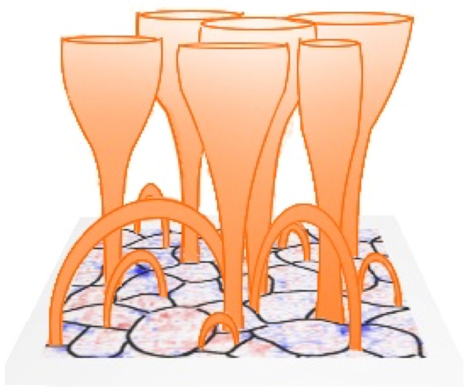
With the objective of constructing a simplified model of the solar atmosphere, we now very briefly recall some of the structures which are actually observed. Our initial computational studies were applicable to quiet Sun regions with magnetic fluxes in the range of 5–10 G, including the non-magnetic solar chromosphere and the quiet inter-network regions between the magnetic flux concentrations. Given the variety of solar atmospheric regions, for example the network, inter-network, plage and faculae regions, it is recognised that the modes of oscillation with periods of 3 and 5 min exhibit varying behaviour. The variation observed for different magnetic structures and reflecting layers such as the transition layer influences propagation in the upward and downward directions. The mean photospheric field in the inter-network region is 100–300 G. On the other hand, flare-producing active regions containing sunspots may have fields easily exceeding the range of 100–500 G. As well as these massive concentrations, solar magnetograms reveal a weak-field component, known as the magnetic carpet. Whilst sunspots may be up to 50 Mm in diameter, solar pores are regions similar to sunspots but with considerably reduced sizes in the range 1–6 Mm. A good discussion of the structure of solar pores can be found in [32,33]. The features considered here are schematically illustrated in Figure 1, which exhibits a variety of network loops with temperatures that can be in the range of K to K; Figure 1 also shows the coronal funnels arising from the areas in-between the solar granules. The dynamic phenomena of concern in this paper result in upward waves and oscillations in the solar atmosphere.
5. Computational Model
The hydrodynamic studies reported in Ref. [25] employed simulation drivers with physical characteristics representing p-mode oscillations with varying modes and periods. The MHD simulations reported here use the same driver and model of the solar atmosphere as used in our initial hydrodynamic study. The model is advanced by the inclusion of a uniform, vertical and cylindrically symmetric magnetic field.
The dimensions of the simulation box are Mm, Mm and a height of Mm in the gravitationally stratified z-direction. The computational box is an array of elements . The upper boundary of the model is in the solar corona whilst the lower boundary is coincident with the photosphere. The MHD code used here is suited to studying the propagation of wave energy from the photosphere, across the transition layer and leaking into the solar corona.
The time scales relevant to our study are determined by the 5-min p-mode oscillations; our approach employs boundary conditions allowing us to model induced wave propagation. To generate these oscillations we use vertical velocity drivers that are extended across the base of the computational domain. The mechanism for handling the boundaries is crucial for maintaining the stability of a simulation over many cycles of the p-mode oscillation. The challenge is to reduce the reflectivity at the boundaries, in particular, the upper and lower boundaries. The method utilised in these simulations attempts to minimise the gradients near the boundary. Since a central difference method is used to compute the gradients, variable values are copied from the mesh edge into two layers of ghost cells. These layers ensure that the discretization method can be applied over the whole mesh. The net result of this approach is that any generated perturbation will be effectively propagated out of the computational domain. This type of boundary condition is referred to as an open boundary condition. In what follows, we describe the model solar atmosphere and the driver employed.
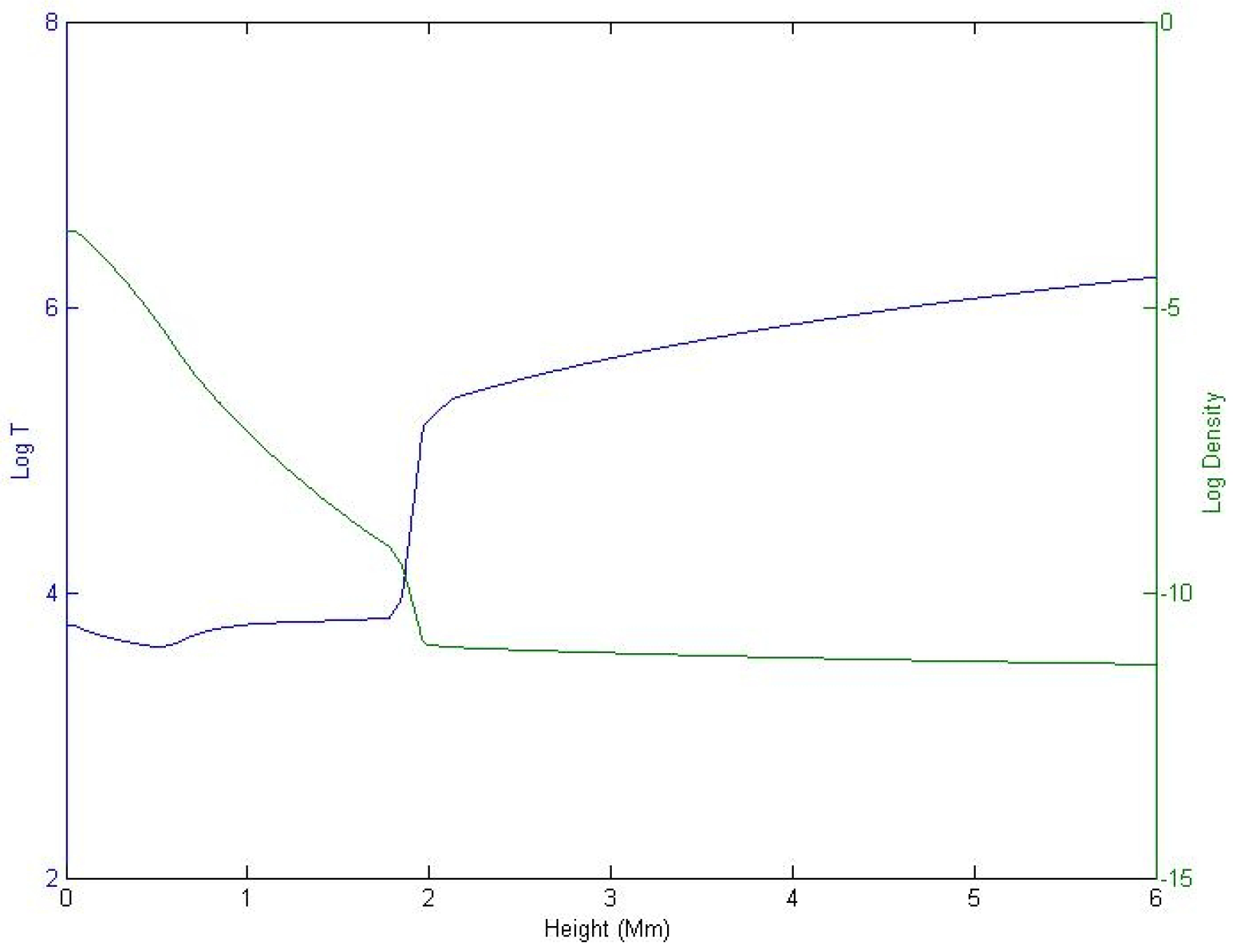
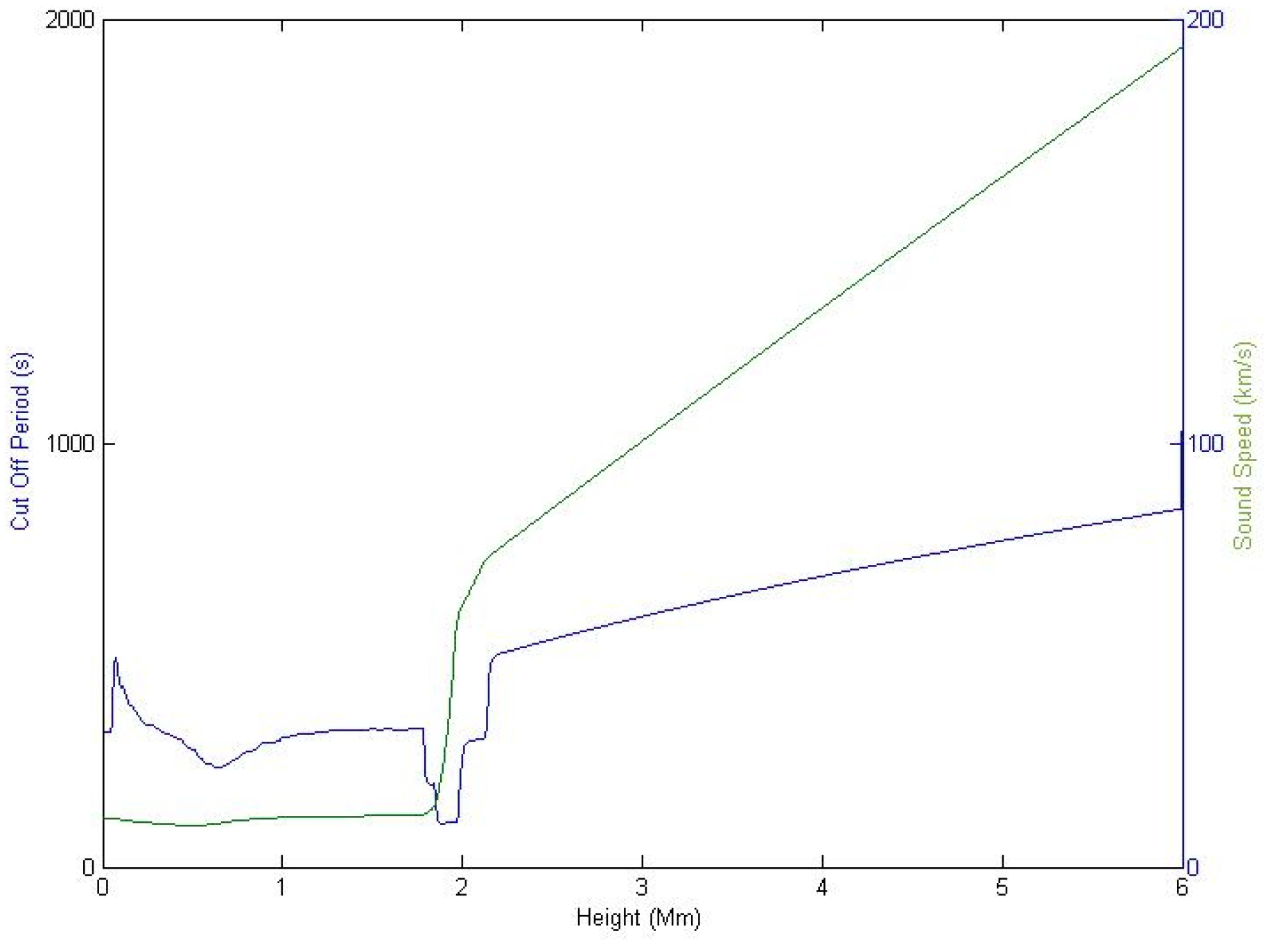
Data obtained from solar observations were used to construct a semi-empirical model solar atmosphere, the resulting model is a representation of the quiet Sun. Employing the fundamental assumption of hydrostatic equilibrium, the VALIIIc model [34] was used to construct a model of the chromosphere in equilibrium. For atmospheric heights greater than 2.5 Mm, the results from a model of solar coronal heating were used [35]. The atmospheric profiles for temperature, density, sound speed and frequency cut-off for this model are shown in Figure 2 and Figure 3.
A further possibility for a model solar atmosphere is the use of the parametric approach; the smoothed step function used in Ref. [36] is an example. Discussion of the validity of model solar atmospheres and realistic models of the chromosphere indicate the need for observationally derived semi-empirical models, see [37,38]. It has been suggested that local dynamo action and joule heating in the dynamical solar chromosphere make the construction of models particularly challenging [39]. The latter aspects are not addressed further in the present study.
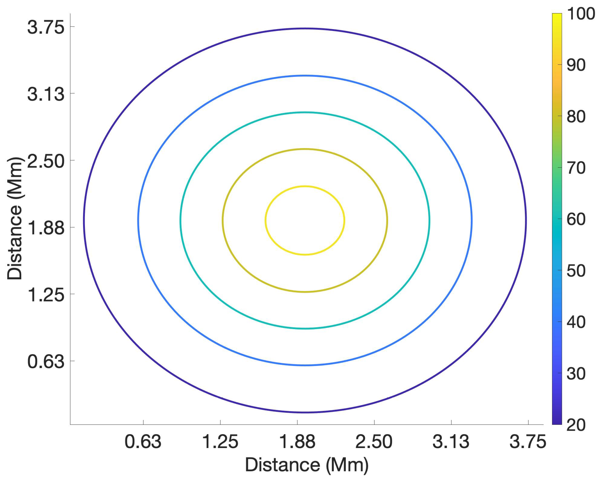
Instead, for the simulations described here, we use a simplistic model that is uniform in the vertical (z) direction. The cylindrically symmetric field was constructed using the parametrisation in Equation (7), the effective cylinder radius was fixed at Mm. Simulations were run for different values of ,
A field configuration with vertical cylindrical symmetry is selected as this provides a working, e.g., rotational symmetry, representation for the weaker intra-network magnetic field. The choice of working geometry is a convenience when coding the MHD equations. The initial magnetic field configuration is shown in Figure 4.
Since the field is uniform in the vertical direction, the model atmosphere is in magnetohydrostatic equilibrium. This was checked by ensuring that the initial configuration satisfies the magnetohydrostatic balance, for an example see [40,41]. We also explicitly tested that the there were no dynamic changes in the model due to a magnetohydrostatic imbalance. The resulting density and temperature profiles are shown in Figure 2.
6. Numerical Drivers for p-Mode Oscillations
The simulations, presented in this paper, employ an extended driver resulting in the perturbation of the entire lower boundary of the model. The photospheric p-mode oscillations that are observed on the Sun have a horizontal wavelength and coherence. The vertical velocity driver used here is an acoustic p-mode driver located at the photosphere and exciting waves which propagate into our realistic 3D model geometry of the solar atmosphere. An extended driver with a sinusoidal dependence and a wavelength of 8 Mm applied along the middle of the base of a computational domain of dimension 4 Mm represents a fundamental mode component of the global acoustic oscillations. Drivers may be constructed as an ensemble of these solar global eigenmodes. The driver is approximated by the expression,
For the simulations here, a p-mode driver corresponding to the 5-min mode was used with period 300 s and mode (2,2) as an example. Earlier studies demonstrated the effectiveness of this mode with energy propagation, see [25]. Simulations were run for different values of the magnitude of the magnetic field. The mode numbers identified here are the n and m values in the expression for the driver shown in Equation (8).
For the driver equation given in Equation (8), is the period, is the amplitude, the indices n and m define the mode and the lengths of the base of the simulation box in the x and y directions are and , respectively. The driver width, is set to 4 km, the parameter was set so that the vertical location of the driver is in the photosphere, 0.5 Mm above the lower boundary of the model and coincident with the location of the temperature minimum. The simulations presented employ the parameter = 500 ms with the mode indices set to .
7. Global Magnetoacoustic Waves in Uniform Vertical Magnetic Field Configurations
Magnetohydrodynamic simulations have been performed with p-mode oscillations of the photospheric layer and for magnetic field strengths of 0 G, 50 G, 75 G and 100 G. The plasma- was determined for the case with a magnetic field strength of 100 G. The plasma- for the model decreases rapidly from a value of 50 at 0.7 Mm above the lower boundary of the simulation domain; is 1 at a height of 1.39 Mm.
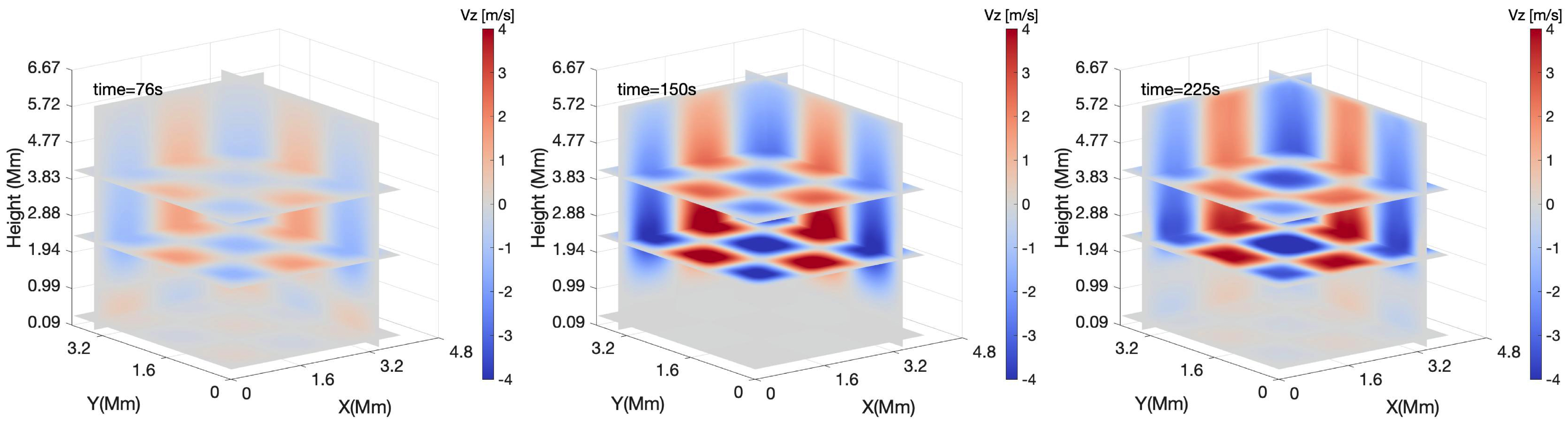
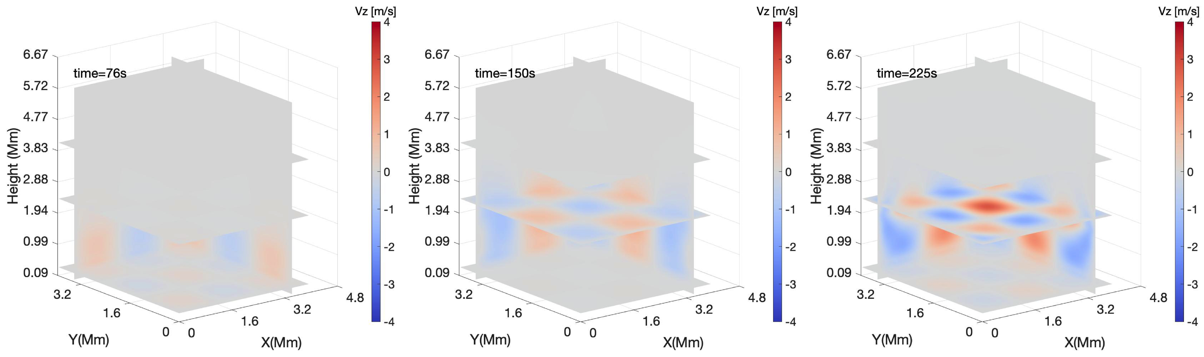
Figure 5 shows the vertical component of the velocity at various times for different sections through the simulation box. Each plot in Figure 5 corresponds to a vertical field configuration with a maximum field strength of 100 G. Figure 6 provides a comparison with the 0 G case and illustrates a clear difference between the purely hydrodynamic and the MHD case. The figures for the MHD case exhibit evidence of a fast moving magnetoacoustic wave mode. The measured propagation speed is consistent with that of a fast magnetoacoustic mode. Figure 5 and Figure 6 compare the wave modes at one-quarter, half and three-quarters of a cycle.
A set of videos of all the simulations that were performed can be obtained from the online research data archive hosted by The University of Sheffield [42]. The videos display the evolution of the z-component of the plasma velocity along different layers of our model solar atmosphere. Each video shows the value of the vertical component of the plasma velocity (z-component in m/s) along different slices through the simulation box. Each video is labelled using the magnetic field strength in Gauss. Inspection of these results reveals that there are channels along which the vertical component of the plasma velocity is enhanced, and these are concentrated towards the central region of the simulation box.
The results obtained indicate that even a small magnetic field appears to enhance the motion of plasma in the low corona and there is an apparent difference in phase between the magnetic field cases. As well as an increase in the velocity amplitude with increasing magnetic field there is a small variation in the frequency of the oscillation. In order to address the observed variation in frequency, further investigative simulations would be required that would include simulations running for a larger number of cycles. The key point here is that the background magnetic field is vertical, one may not accept any frequency variation assuming a linear wave evolution is the key component to the physics. Since the simulations do show small frequency variations, this may mean that that the linear theory may break.
After much effort implementing and testing the chosen numerical scheme to solve the numerical equations, there are still reflections at the boundary; therefore, we consider the simulations to be valid up to the point where reflection occurs. Because of this, the simulations are cut after approximately 600 s of real time, corresponding to two period cycles.
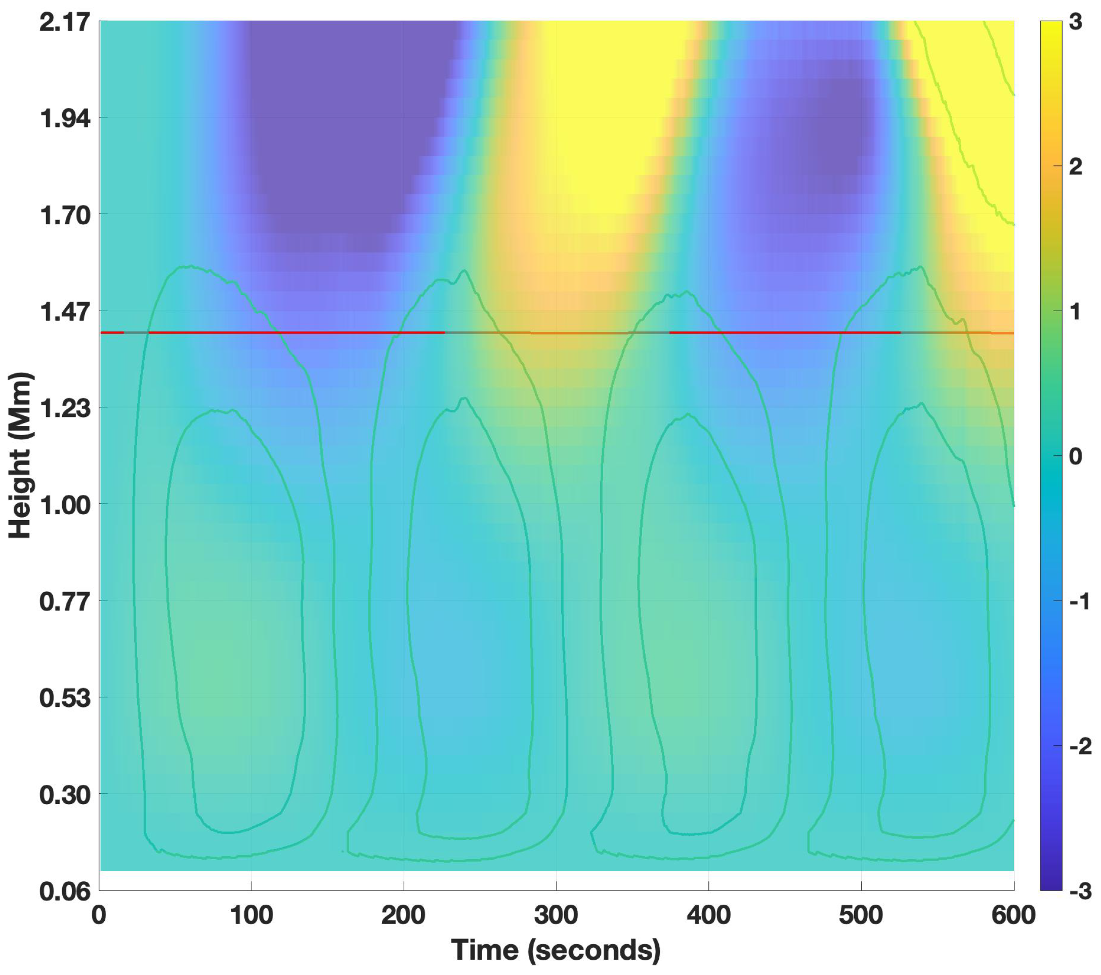
A time–distance plot for the 300 s period driver, with the 100 G field is shown in Figure 7. The reflections from the imperfect boundary conditions result in increased velocity amplitudes after a few oscillations. Although we are investigating the propagation of waves into the corona, the time–distance plots emphasise phenomena observed in the chromosphere and around the transition zone. The wave speeds measured from this time–distance plot are shown in Table 1. A comparison with the wave speeds computed from the model atmosphere suggests that the speeds for the 0 G field are consistent with the speed of sound in the solar atmosphere, whilst the speeds for the non-zero magnetic field are consistent with propagation speeds for magnetosonic modes. For a vertical magnetic flux with magnetic field strength and internal density , comparisons with the measured wave speeds were computed using the following definitions: the speed of sound,
the Alfvén speed,
the magnetoacoustic wave speeds, also known as the slow or cusp or tube speed,
and the kink speed,
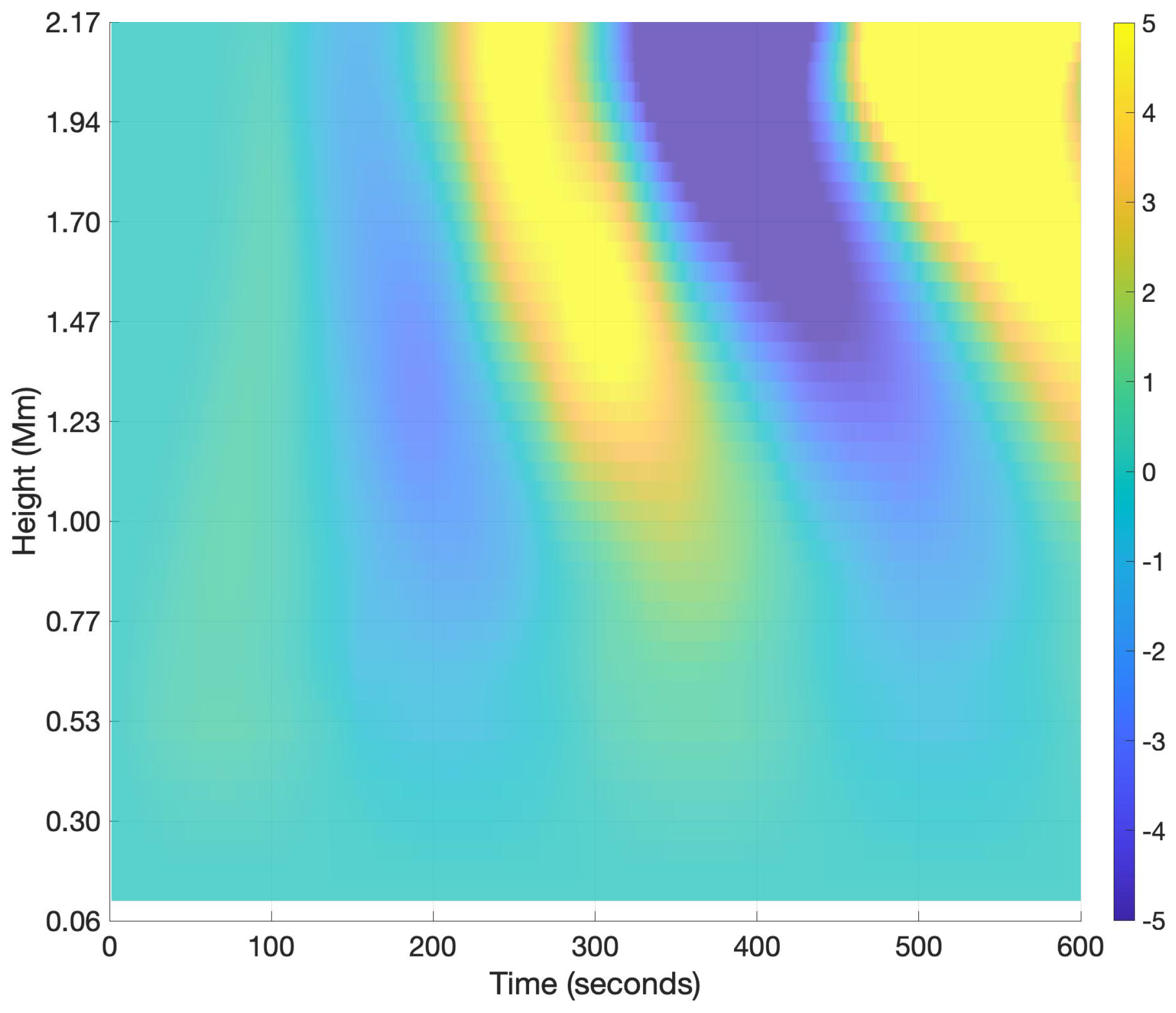
The results indicate a variety of waves. Inspection of Figure 8 reveals excitation from the driver along with quasi-standing oscillations in the chromospheric cavity. There is also partial reflection of the signal at the boundary of the chromosphere and the transition layer. The results also display evidence for signals propagating horizontally at the transition region and with frequencies similar to that of the driver. The time–distance plot in Figure 7, for the 100 G case, exhibits reduced reflection at the transition layer, indicating energy leakage into the solar corona. Figure 7 shows an initial fast mode pulse followed by slow mode oscillations above the line which correspond to a plasma- with a value of one. Below the height of 1 Mm, we observe quasi-standing mode oscillations along with oscillations of the magnetic field perturbations. Below 0.3 Mm, the driver oscillations can be observed in conjunction with possible magnetoacoustic slow mode oscillations. Since the source terms perturb only the vertical component of the velocity and the model is cylindrically symmetric, pure Alfvén modes are not expected.
The time–distance plots displaying the vertical component of the plasma velocity indicate significant differences in the propagation behaviour for the hydrodynamic and non-zero magnetic field cases. It is necessary to understand and quantify the extent of the energy leakage into the solar atmosphere. To investigate the influence of the magnetic field on the propagation of wave energy we employ an expression for the energy flux which was used by [43]. The wave energy flux is given by
The perturbed variables are represented with a tilde on top of the variable and a subscript b for the background variables.
We compute the time-averaged energy flux integrated over different cross sections of the simulation box:
These expressions are dependent on the perturbed kinetic pressure ,
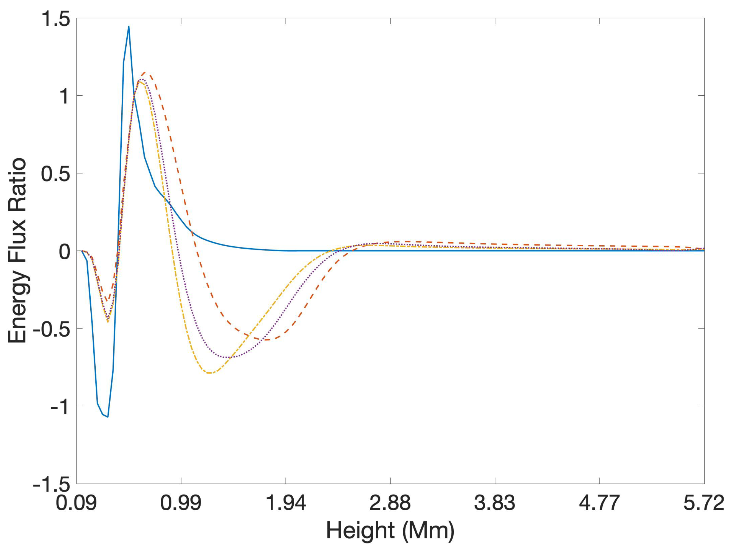
Using Equation (13), we computed the energy flux integral for each of the drivers at different atmospheric heights and averaged over the total time. Next, we compute the ratio of this integrated energy flux to the integrated energy flux at the location of the driver. The resulting values are shown in Table 2. It appears that for heights greater than 4 Mm, the energy flux is enhanced for increasing values for the vertical magnetic field. In Figure 9, we plot the ratio of the integrated energy flux ratio for different values of the field at different heights and for the different vertical field values (the blue, orange, purple and red are for field values of 0 G, 50 G, 75 G and 100 G, respectively). These plots demonstrate that for higher B-field magnitudes there is a small leakage of energy propagation. This latter finding is interesting because this is consistent with observations and other simulation results that demonstrate an enhancement for inclined fields.
8. Frequency Analysis
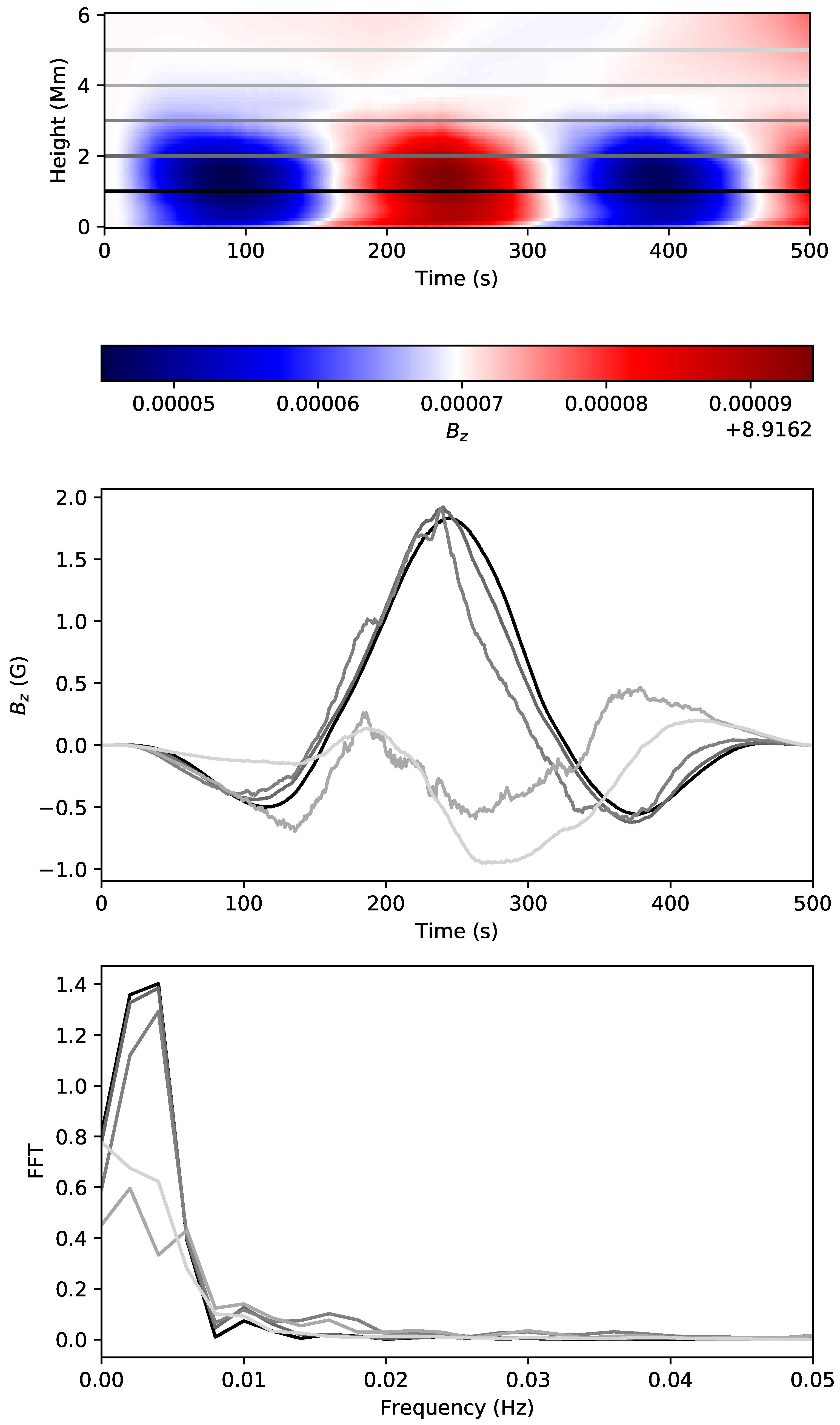
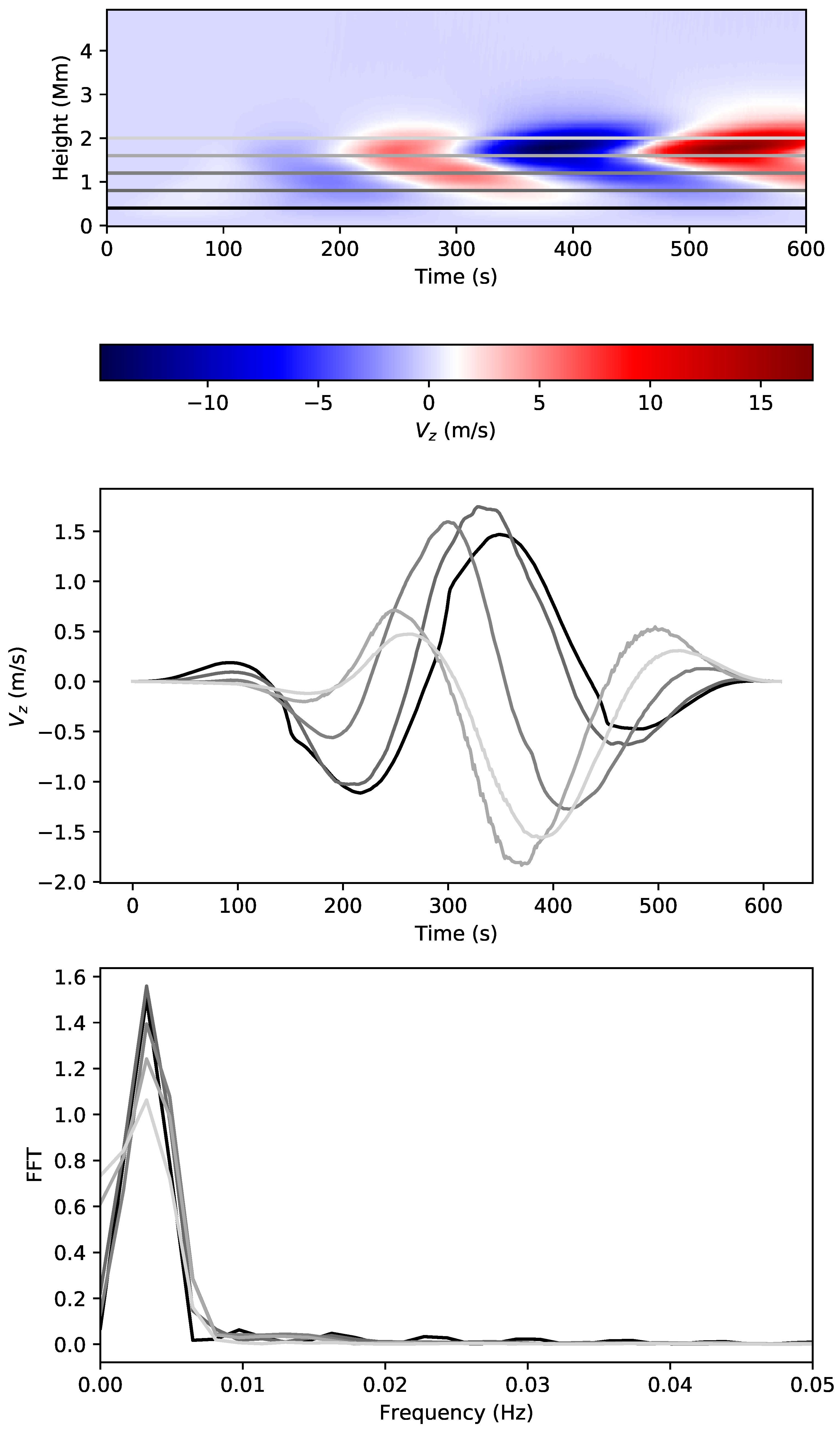
We analysed the temporal behaviour of the numerical results, outlined in the previous section. Figure 10 (top) shows a vertical slice of over time. The data are based on the simulation with the initial magnetic field configuration with a maximum value of 100 G. From this two-dimensional plane, five layers were selected, representing different heights in the solar atmosphere. The layers are indicated by the horizontal grey lines. Figure 10 (middle) displays the temporal variation of the selected layers, indicated by different grey shade colours. A fast Fourier transform (FFT) was applied (see Figure 10 (bottom)) for investigating any oscillatory behaviour in the analysed signal. A significant oscillatory pattern was found with frequency range of 3.75–4 mHz, corresponding to a period range of 4.2–4.4 min. A slight frequency variation is also recognisable. The different layers in height tend to feature variations in the peak positions identified from the FFT analysis. An FFT was also performed based on the other simulations with different initial magnetic field configurations (with a maximum value of 0 G, 50 G, 75 G and 100 G). These investigations all showed similar oscillatory behaviour. Figure 11 features the same analysis as Figure 10; however, the study features a vertical slice of over time. The analysis shows similar properties as the data based on a vertical slice of .
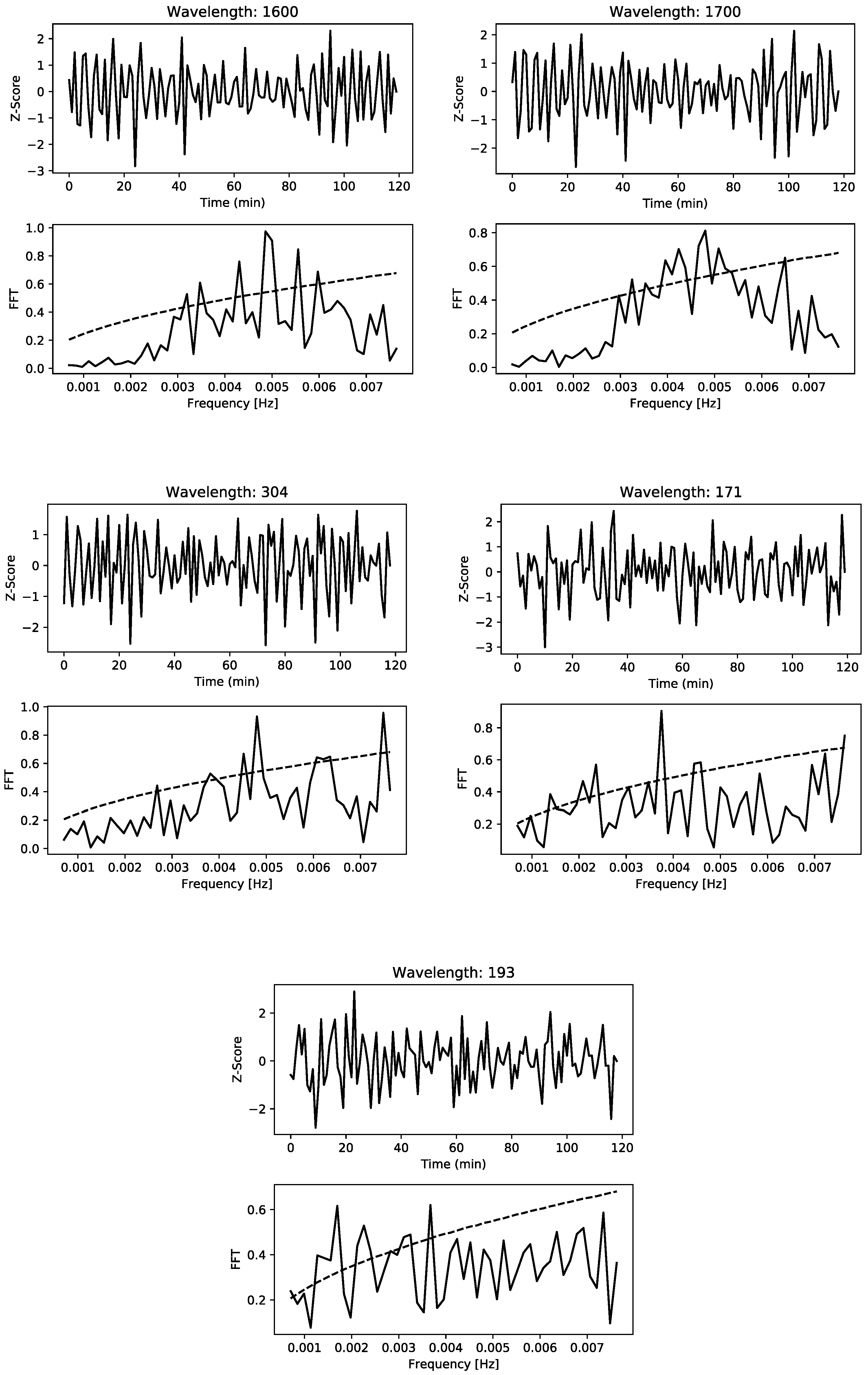
With the objective of confirming the obtained oscillatory behaviour, temporal analysis for the observational data [44,45] was performed. We investigated intensity oscillations in the solar atmosphere observed by SDO/AIA (Atmospheric Imaging Assembly) [45]. The passbands 1600 Å, 1700 Å, 304 Å, 171 Å and 193 Å were selected because our simulation mainly focused on the lower atmospheric regions, i.e., photosphere, chromosphere and low corona. The cadence of images is 24 s; therefore, it was suitable for studying relatively high-frequency oscillations such as the obtained 4 mHz.
The initial magnetic field configuration of our model is a standing magnetic tube, passing through the chromosphere and the lower corona. The selected area contains a small sunspot (e.g., a solar pore), presumably featuring similar magnetic structure as our simulation. The size of the investigated area covers 50 pixels in total between 18:00 UT to 20:00 UT on 22 August 2010. The obtained time series shows non-stationary behaviour; therefore, the observed linear trend is removed by taking the first difference of the data. The first difference is defined as the difference between consecutive observations and . Furthermore, the times series is also normalised by applying standard scores (Z-scores), defined by
where, the parameter is the mean of the time series and the parameter is defined as the standard deviation of the data. Figure 12 demonstrates the trend removed and normalised time series (Z-scores) and shows the result of the applied FFT technique. The dashed line is the significance level () which was calculated using a Monte Carlo method. The original data showed red noise signature which transformed to blue noise after differentiating the data. We have generated 1 million blue noise signatures, , and calculated the standard deviation, , and the mean, , of the simulated noise, providing our significance level S:
The results of the analyses are summarised in Table 3. A significant period is found with a frequency range of 3.5–4.2 mHz, corresponding a period range of 4.7–4 min, which is close to the period found in simulation data. Another significant peak (5 mHz) is found with a period around 3 min, which may be an indication of another global oscillation. This randomly selected region in the solar surface suggests that the observed oscillation is a global phenomenon.
9. Discussion
Whilst many studies focus on local wave phenomena, the simulations and observational analysis reported here are attempting to address the global oscillations of the solar atmosphere from the photosphere into the low corona. These ubiquitous oscillations result in a small but detectable leakage of energy from the chromosphere into the coronal regions of the solar atmosphere. It is worth noting that this energy may not be adequate to heat these regions to the observed temperatures. However, addressing the known solar atmospheric plasma heating is not the main concern of this paper. Its purpose is to show that these global oscillations are present, and just like in the inner regions or for coronal loops, they may be explored for magneto-seismology.
Early theoretical studies considered wave propagation in idealised magnetic slab structures and demonstrated the fundamental conditions for MHD wave propagation [46,47]. These models were soon advanced to cylindrical magnetic structures and addressed the different types of MHD waves sustained under the conditions of the solar corona [48]. Investigation of the propagation of magnetoacoustic oscillations in an isothermal atmosphere with a vertical magnetic field resulted in the prediction of small frequency shifts of solar global internal or acoustic oscillations, see, e.g., [49]. The analysis was unable to demonstrate the absorption of MHD waves, for example as observed in sunspots. Many of these earlier studies focused on the effect of magnetic flux tubes on wave propagation and neglected gravitational stratification. Much effort has been made to understand the role of solar atmospheric oscillations in coronal heating. Such modelling has ranged from one dimensional models modelling radiative energy loss to taking into account two fluid models of the plasma. Further work investigated the influence of vertical fields on a variety of modes, including p-mode oscillations in an isothermal stratified atmosphere [50]. In the limit of weak fields these results were used to analyse the spectrum of the modes of oscillation for the stratified atmosphere.
The review [27] considered localised wave phenomena and variation in different magnetic structures of the quiet Sun. For example, in the close proximity of the magnetic network elements, the longer 5-min modes propagate efficiently to the chromosphere. The 3-min modes propagate from the photosphere to the chromosphere in the network cell interiors for restricted regions of the network and internetwork. Observations show that the 3-min modes exhibit enhancement in both the photosphere and the chromosphere, whereas the power of the 5-min modes increases significantly in the chromosphere. These power enhancements are known as ”halos” and have been well reported [51]. In contrast, the work reported here is an extension of an earlier study representing photospheric p-mode oscillations using different point drivers [52]. These studies demonstrated the generation of surface waves, structures in the transition zone and identified the effect of cut-offs induced by the stratified solar atmosphere. The brief overview in Section 2 identified the physical phenomena of leaking energy into the lower solar atmosphere and the resulting oscillatory behaviour there.
An initial study of global oscillations in a highly gravitationally stratified atmosphere looked at the variation of energy leakage with different modes of oscillation of an extended driver [25]. The investigation addressed an observational study indicating the ubiquitous nature of intensity oscillations. The power spectra presented in Figure 1 of Ref. [25] exhibit a variation of propagation characteristics at different levels within the solar atmosphere and within different regions such as coronal holes, the quiet Sun and active regions. The power spectra indicate a preponderance of long-period 5-min waves with frequencies in the range of 1.5–5 mHz. Furthermore, observed are the distinctive peaks for the short-period 3-min waves (with frequencies in the range of 5–8 mHz). The power spectra exhibit peaks in much longer period ranges, for example 12-min waves (frequencies in the range 1.1–1.5 mHz) and 16-min waves (frequencies 1–1.1 mHz). For the quiet Sun regions the 5-min modes are stronger at photospheric levels and diminished higher up in the corona; there is a small peak for the data from the AIA passband at 211 Å corresponding to the corona at 2.0 MK. The computational results presented here corroborate the suggestion of [53] of the existence of global oscillations in the solar corona. The suggestion of small energy deposition events was indicated by [54] in their study of power spectra of the solar corona. They suggest that this is the result of the summation of energy deposition events in the solar atmosphere.
The remaining study focused on global oscillations of the solar atmosphere and employing extended drivers to emulate a driving p-mode oscillation. The initial work with a hydrodynamic model was extended into an idealised model of a typical solar pore. Further, as a test of ubiquity, the observational analysis has been for randomly selected regions and the Fourier analysis for the observational results has been compared to a similar analysis for the simulated feature.
10. Conclusions
In this paper, we have presented results for a series of MHD simulations of an extended oscillator at the base of a simple model solar atmosphere. A comparison with observational data provides a unique insight into the nature of global oscillations in the upper solar atmosphere caused by the ubiquitous p-mode oscillation. It was found that the oscillations are enhanced by a vertical magnetic field. Although the observational data suggest that the global atmospheric oscillations are detectable through oscillations in intensity, the small energy leakage is not sufficient for heating of the solar corona; this is supported by the results of the simulations.
We have successfully extended the initial hydrodynamic model of global oscillations to test how the SMAUG [29] code works when our model atmosphere includes an initially symmetric and uniform magnetic field. Accelerated MHD codes such as SMAUG are a key requirement for simulations of magnetic and highly stratified plasma which are run for long time periods, for example, for models of the solar global oscillations. As attempts are made to model large scale and more complex regions of the solar atmosphere, multiple graphical processing units will be required.
The simulations with an extended driver show that the observed solar atmospheric global oscillations are enhanced by regions with a vertical magnetic field. Investigation of the energy flux propagation results are indicative of the enhanced propagation of energy with increasing magnetic fields, but this is not sufficient to result in significant solar coronal heating. The analysis suggests that the energy propagation is by magnetosonic modes. Due to the steep density changes around the transition region, slow and fast magnetosonic modes are responsible for reflecting some energy back to the chromosphere and the photosphere.
The FFT analysis of the simulated data demonstrated the presence of oscillations with periods in the range of 4.2–4.4 min. This arose for both the hydrodynamic case and the case with a magnetic field of 100 G. In the latter case there was some additional structure for the FFT analysis. There is a clear variation of the oscillation frequency around the 5 min period of the driver.
It is interesting that there is a similarity between the FFT analysis of simulations and observations for different solar features, for example for the quiet Sun or for regions with pores. The results, derived from intensity time series of SDO images, also exhibit a significant variation of the oscillation frequency from the period of the global 5-min oscillation. The frequency variation is larger than would be expected from simple (e.g., linear) theory. Such frequency variations may be attributed to additional elasticity in the solar atmosphere resulting from the presence of a magnetic field, from non-linear processes or from the artefacts of the observational method. This may be understood in part by referring to Ref. [55]; however, in their model the magnetic field was horizontal. An explanation based on the study of Ref. [49] does not seem to explain the size of the frequency variations found in the simulations.
Care must be taken with the measurement of the simulated frequency variation, and further work is required to provide more insight into the different mechanisms. An example could be a result of the superposition of waves arriving at different heights and times, such a mechanism allows for the spatio-temporal variation of the magnetic field. Improved boundary conditions handling reflections from the upper boundary will be required to run simulations for much longer time intervals and with inclined magnetic fields. A further consideration may be a comparison of the results from the vertical tube with a model which is an improved representation of a solar pore [32,33].
It is encouraging that the results presented here are consistent with the behaviour exhibited by earlier studies. There is an issue that due to the extended nature of the driver, the amplitudes are responsible for delivering vast quantities of energy into the solar atmosphere inducing extremely large shocks and result in a numerically unstable system [26]. Significant improvements to the comparisons presented in this paper are expected with the recent study of Ref. [56]. Here, using the ADIPLS code [57], a model of the intensity perturbations using a VALIIIc solar atmosphere model with radiative transfer was used to simulate the intensity oscillations perturbed by the solar global oscillations. As described in Ref. [58], more sensitive observations with instruments such as DKIST (the Daniel K. Inouye Solar Telescope) may enable further constraints on the range of theoretical models.
Author Contributions
Conceptualisation, M.G., N.G., R.Z., M.K. and R.E.; methodology, M.G., N.G. and R.E.; software, M.G. and N.G.; validation, M.G. and N.G.; formal analysis, M.G., N.G. and R.E.; writing—original draft preparation, M.G.; writing—review and editing, M.G., N.G., M.K. and R.E.; visualisation, M.G. and N.G.; preparation of Figure 1, M.K.; supervision, R.E.; funding acquisition, R.E. All authors have read and agreed to the published version of the manuscript.
Funding
This research was funded by the UK, Science and Technology Facilities Council (STFC) (grant number ST/M000826/1). R.E. acknowledges the support received from the Royal Society (UK). R.E. also acknowledges support from the European Union’s Horizon 2020 research and innovation programme under the grant agreements no. 739500 (PRE-EST project) and no. 824135 (SOLARNET project). M.K. is grateful to ST/S000518/1, PIA.CE.RI. 2020-2022 Linea2, CESAR 2020-35-HH.0, and UNKP-22-4-II-ELTE-186 grants (UK). R.E. and M.K. are also grateful to NKFIH, National Research and Innovation Office (OTKA, the Hungarian Scientific Research Fund, grant No. K142987), Hungary, for enabling this research.
Data Availability Statement
The data used can be obtained in the references cited and on request from the corresponding author.
Acknowledgments
The authors thank P.H. Keys for providing the wavelet tools to analyse the related SDO data. We acknowledge IT Services at The University of Sheffield for the provision of the high performance computing service.
Conflicts of Interest
The authors declare no conflict of interest. The funders had no role in the design of the study; in the collection, analyses, or interpretation of data; in the writing of the manuscript; or in the decision to publish the results.
Abbreviations
The following abbreviations are used in this manuscript:
| AIA | Atmospheric Imaging Assembly |
| DKIST | the Daniel K. Inouye Solar Telescope |
| FFT | fast Fourier transform |
| GPU | graphical processing unit |
| MHD | magnetohydrodynamics |
| SDO | Solar Dynamics Observatory |
| SMAUG | Sheffield magnetohydrodynamics accelerated using GPUs |
| VAC | Versatile Advection Code |
| VALIIIc | Vernazza, Avrett and Loeser |
| 1D, 2D, 3D | one-, two-, three-dimensional |
References
- Erdélyi, R. Magnetic coupling of waves and oscillations in the lower solar atmosphere: Can the tail wag the dog? Philos. Trans. R. Soc. A Math. Phys. Eng. Sci. 2005, 364, 351–381. [Google Scholar] [CrossRef]
- Taroyan, Y.; Erdélyi, R. Global acoustic resonance in a stratified solar atmosphere. Sol. Phys. 2008, 251, 523–531. [Google Scholar] [CrossRef]
- Pintér, B.; Erdélyi, R.; Goossens, M. Global oscillations in a magnetic solar model. Astron. Astrophys. 2007, 466, 377–388. [Google Scholar] [CrossRef]
- Mein, N.; Mein, P. Velocity waves in the quiet solar chromosphere. Sol. Phys. 1976, 49, 231–248. [Google Scholar] [CrossRef]
- Schmieder, B.; Mein, N. Mechanical flux in the solar chromosphere. II. Determination of the mechanical flux. Astron. Astrophys. 1980, 84, 99–105. Available online: https://ui.adsabs.harvard.edu/abs/1980A%26A....84...99S/ (accessed on 18 March 2023).
- De Moortel, I. Longitudinal waves in coronal loops. Space Sci. Rev. 2009, 149, 65–81. [Google Scholar] [CrossRef]
- Banerjee, D.; Gupta, G.R.; Teriaca, L. Propagating MHD waves in coronal holes. Space Sci. Rev. 2010, 158, 267–288. [Google Scholar] [CrossRef]
- Mathioudakis, M.; Jess, D.; Erdélyi, R. Alfvén waves in the solar atmosphere. Space Sci. Rev. 2012, 175, 1–27. [Google Scholar] [CrossRef]
- Ruderman, M.S.; Erdélyi, R. Transverse oscillations of coronal loops. Space Sci. Rev. 2009, 149, 199–228. [Google Scholar] [CrossRef]
- Wang, T. Standing slow-mode waves in hot coronal loops: Observations, modeling, and coronal seismology. Space Sci. Rev. 2011, 158, 397–419. [Google Scholar] [CrossRef]
- Auchère, F.; Bocchialini, K.; Solomon, J.; Tison, E. Long-period intensity pulsations in the solar corona during activity cycle 23. Astron. Astrophys. 2014, 563, A8. [Google Scholar] [CrossRef]
- Jensen, E.; Orrall, F.Q. Observational study of macroscopic inhomogeneities in the solar atmosphere. IV. Velocity and intensity fluctuations observed in the K line. Astrophys. J. 1963, 138, 252–270. [Google Scholar] [CrossRef]
- Banerjee, D.; Erdélyi, R.; Oliver, R.; O’Shea, E. Present and future observing trends in atmospheric magnetoseismology. Sol. Phys. 2007, 246, 3–29. [Google Scholar] [CrossRef]
- Erdélyi, R.; Taroyan, Y. Hinode EUV spectroscopic observations of coronal oscillations. Astron. Astrophys. 2008, 489, L49–L52. [Google Scholar] [CrossRef]
- Roberts, B.; Edwin, P.M.; Benz, A. On coronal oscillations. Astrophys. J. 1984, 279, 857–865. [Google Scholar] [CrossRef]
- Verth, G.; Erdélyi, R.; Goossens, M. Magnetoseismology: Eigenmodes of torsional Alfvén waves in stratified solar waveguides. Astrophys. J. 2010, 714, 1637–1648. [Google Scholar] [CrossRef]
- Zaqarashvili, T.V.; Murawski, K. Torsional oscillations of longitudinally inhomogeneous coronal loops. Astron. Astrophys. 2007, 470, 353–357. [Google Scholar] [CrossRef]
- Gyenge, N.; Erdélyi, R. Periodic recurrence patterns in X-Ray solar flare appearances. Astrophys. J. 2018, 859, 169. [Google Scholar] [CrossRef]
- Gudiksen, B.V.; Carlsson, M.; Hansteen, V.H.; Hayek, W.; Leenaarts, J.; Martínez-Sykora, J. The stellar atmosphere simulation codeBifrost. Astron. Astrophys. 2011, 531, A154. [Google Scholar] [CrossRef]
- Vögler, A.; Shelyag, S.; Schüssler, M.; Cattaneo, F.; Emonet, T.; Linde, T. Simulations of magneto-convection in the solar photosphere. Equations, methods, and results of the MURaM code. Astron. Astrophys. 2005, 429, 335–351. [Google Scholar] [CrossRef]
- Zhang, F.; Poedts, S.; Lani, A.; Kuźma, B.; Murawski, K. Two-fluid modeling of acoustic wave propagation in gravitationally stratified isothermal media. Astrophys. J. 2021, 911, 119. [Google Scholar] [CrossRef]
- Fedun, V.; Erdélyi, R.; Shelyag, S. Oscillatory response of the 3D solar atmosphere to the leakage of photospheric motion. Sol. Phys. 2009, 258, 219–241. [Google Scholar] [CrossRef]
- Fedun, V.; Shelyag, S.; Verth, G.; Mathioudakis, M.; Erdélyi, R. MHD waves generated by high-frequency photospheric vortex motions. Ann. Geophys. 2011, 29, 1029–1035. [Google Scholar] [CrossRef]
- Vigeesh, G.; Fedun, V.; Hasan, S.S.; Erdélyi, R. Three-dimensional simulations of magnetohydrodynamic waves in magnetized solar atmosphere. Astrophys. J. 2012, 755, A18. [Google Scholar] [CrossRef]
- Griffiths, M.; Fedun, V.; Erdélyi, R.; Zheng, R. Solar atmosphere wave dynamics generated by solar global oscillating eigenmodes. Adv. Space Res. 2018, 61, 720–737. [Google Scholar] [CrossRef]
- Santamaria, I.C.; Khomenko, E.; Collados, M. Magnetohydrodynamic wave propagation from the subphotosphere to the corona in an arcade-shaped magnetic field with a null point. Astron. Astrophys. 2015, 577, A70. [Google Scholar] [CrossRef]
- Khomenko, E.; Calvo Santamaria, I. Magnetohydrodynamic waves driven by p-modes. J. Phys. Conf. Ser. 2013, 440, 012048. [Google Scholar] [CrossRef]
- Shelyag, S.; Fedun, V.; Erdélyi, R. Magnetohydrodynamic code for gravitationally-stratified media. Astron. Astrophys. 2008, 486, 655–662. [Google Scholar] [CrossRef]
- Griffiths, M.K.; Fedun, V.; Erdélyi, R. A Fast MHD code for gravitationally stratified media using graphical processing units: SMAUG. J. Astrophys. Astron. 2015, 36, 197–223. [Google Scholar] [CrossRef]
- Tóth, G. A General code for modeling MHD flows on parallel computers: Versatile Advection Code. Astrophys. Lett. Commun. 1996, 34, 245–250. Available online: https://ui.adsabs.harvard.edu/abs/1996ApL%26C..34..245T (accessed on 18 March 2023).
- Caunt, S.E.; Korpi, M.J. A 3D MHD model of astrophysical flows: Algorithms, tests and parallelisation. Astron. Astrophys. 2001, 369, 706–728. [Google Scholar] [CrossRef]
- Simon, G.W.; Weiss, N.O. On the magnetic field in pores. Sol. Phys. 1970, 13, 85–103. [Google Scholar] [CrossRef]
- Cameron, R.; Schüssler, M.; Vögler, A.; Zakharov, V. Radiative magnetohydrodynamic simulations of solar pores. Astron. Astrophys. 2007, 474, 261–272. [Google Scholar] [CrossRef]
- Vernazza, J.E.; Avrett, E.H.; Loeser, R. Structure of the solar chromosphere. III. Models of the EUV brightness components of the quiet-sun. Astrophys. J. Suppl. Ser. 1981, 45, 635–725. [Google Scholar] [CrossRef]
- McWhirter, R.W.P.; Thonemann, P.C.; Wilson, R. The heating of the solar corona. II. A model based on energy balance. Astron. Astrophys. 1975, 40, 63–73. Available online: https://ui.adsabs.harvard.edu/abs/1975A%26A....40...63M/ (accessed on 18 March 2023).
- Murawski, K.; Zaqarashvili, T.V. Numerical simulations of spicule formation in the solar atmosphere. Astron. Astrophys. 2010, 519, A8. [Google Scholar] [CrossRef]
- Kalkofen, W. The validity of dynamical models of the solar atmosphere. Sol. Phys. 2011, 276, 75–95. [Google Scholar] [CrossRef]
- Carlsson, M.; Stein, R.F. Does a nonmagnetic solar chromosphere exist? Astrophys. J. Lett. 1995, 440, L29–L32. [Google Scholar] [CrossRef]
- Leenaarts, J.; Carlsson, M.; Hansteen, V.; Gudiksen, B.V. On the minimum temperature of the quiet solar chromosphere. Astron. Astrophys. 2011, 530, A124. [Google Scholar] [CrossRef]
- Gent, F.A.; Fedun, V.; Mumford, S.J.; Erdélyi, R. Magnetohydrostatic equilibrium—I. Three-dimensional open magnetic flux tube in the stratified solar atmosphere. Mon. Not. R. Astron. Soc. 2013, 435, 689–697. [Google Scholar] [CrossRef]
- Schüssler, M.; Rempel, M. The dynamical disconnection of sunspots from their magnetic roots. Astron. Astrophys. 2005, 441, 337–346. [Google Scholar] [CrossRef]
- Griffiths, M.; von Fay-Siebenburgen, R.; Erdélyi. Videos of p-Mode Oscillations in Highly Gravitationally Stratified Magnetic Solar Atmospheres. The University of Sheffield. 2018. Available online: https://figshare.shef.ac.uk/articles/dataset/Videos_of_p-Mode_Oscillations_in_Highly_Gravitationally_Stratified_Magnetic_Solar_Atmospheres/7378046 (accessed on 18 March 2023).
- Bogdan, T.J.; Hansteen, M.C.V.; McMurry, A.; Rosenthal, C.S.; Johnson, M.; Petty, S.; Zita, E.J.; Stein, R.F.; McIntosh, S.W.; Nordlund, P. Waves in the magnetized solar atmosphere. II. Waves from localized sources in magnetic flux concentrations. Astrophys. J. 2003, 599, 626–660. [Google Scholar] [CrossRef]
- Pesnell, W.D.; Thompson, B.J.; Chamberlin, P.C. The Solar Dynamics Observatory (SDO). Sol. Phys. 2012, 275, 3–15. [Google Scholar] [CrossRef]
- Lemen, J.R.; Title, A.M.; Akin, D.J.; Boerner, P.F.; Chou, C.; Drake, J.F.; Duncan, D.W.; Edwards, C.G.; Friedlaender, F.M.; Heyman, G.F.; et al. The Atmospheric Imaging Assembly (AIA) on the Solar Dynamics Observatory (SDO). Sol. Phys. 2012, 275, 17–40. [Google Scholar] [CrossRef]
- Roberts, B. Wave propagation in a magnetically structured atmosphere. I: Surface waves at a magnetic interface. Sol. Phys. 1981, 169, 27–38. [Google Scholar] [CrossRef]
- Roberts, B. Wave propagation in a magnetically structured atmosphere. II: Waves in a magnetic slab. Sol. Phys. 1981, 69, 39–56. [Google Scholar] [CrossRef]
- Edwin, P.M.; Roberts, B. Wave propagation in a magnetic cylinder. Sol. Phys. 1983, 88, 179–191. [Google Scholar] [CrossRef]
- Hindman, B.; Zweibel, E.G.; Cally, P. Driven acoustic oscillations within a vertical magnetic field. Astrophys. J. 1996, 459, 760–772. [Google Scholar] [CrossRef]
- Hasan, S.S.; Christensen-Dalsgaard, J. The influence of a vertical magnetic field on oscillations in an isothermal stratified atmosphere. Astrophys. J. 1992, 396, 311–332. [Google Scholar] [CrossRef]
- Kontogiannis, I.; Tsiropoula, G.; Tziotziou, K. Power halo and magnetic shadow in a solar quiet region observed in the Hα line. Astron. Astrophys. 2010, 510, A41. [Google Scholar] [CrossRef]
- Malins, C. On transition region convection cells in simulations of p-mode propagation. Astron. Notes/Astron. Nachr. 2007, 328, 752–755. [Google Scholar] [CrossRef]
- Didkovsky, L.; Kosovichev, A.; Judge, D.; Wieman, S.; Woods, T. Variability of solar five-minute oscillations in the corona as observed by the Extreme Ultraviolet Spectrophotometer (ESP) on the Solar Dynamics Observatory/Extreme Ultraviolet Variability Experiment (SDO/EVE). Sol. Phys. 2012, 287, 171–184. [Google Scholar] [CrossRef]
- Ireland, J.; McAteer, R.T.J.; Inglis, A. Coronal fourier power spectra: Implications for coronal seismology and coronal heating. Astrophys. J. 2015, 798, 1. [Google Scholar] [CrossRef]
- Campbell, W.R.; Roberts, B. The influence of a chromospheric magnetic field on the solar p- and f-modes. Astrophys. J. 1989, 338, 538–556. [Google Scholar] [CrossRef]
- Kostogryz, N.M.; Fournier, D.; Gizon, L. Modelling continuum intensity perturbations caused by solar acoustic oscillations. Astron. Astrophys. 2021, 654, A1. [Google Scholar] [CrossRef]
- Christensen-Dalsgaard, J. ADIPLS—The Aarhus adiabatic oscillation package. Astrophys. Space Sci. 2008, 316, 113–120. [Google Scholar] [CrossRef]
- Rast, M.; Martinez Pillet, V. Resolving the Source of the Solar Acoustic Oscillations: What Will Be Possible with DKIST? AAS/Solar Physics Division Abstracts #47. 2016. Available online: https://ui.adsabs.harvard.edu/abs/2016SPD....4720105R%2F (accessed on 18 March 2023).
Figure 1.
A schematic representation of the solar magnetic network. See text for details.

Figure 2.
Atmospheric profiles for the density and temperature for the model solar atmosphere based on the VALIIIc model [34].
Figure 2.
Atmospheric profiles for the density and temperature for the model solar atmosphere based on the VALIIIc model [34].

Figure 3.
Profiles of the computed speed of sound and the frequency cut-off for a solar model atmosphere based on the VALIIIc model [34].
Figure 3.
Profiles of the computed speed of sound and the frequency cut-off for a solar model atmosphere based on the VALIIIc model [34].

Figure 4.
The initial magnetic field configuration showing the radial field distribution that is cylindrical and uniform in the vertical direction with a maximum value of 100 G. The color bar shows the magnetic field strength in Gauss.
Figure 4.
The initial magnetic field configuration showing the radial field distribution that is cylindrical and uniform in the vertical direction with a maximum value of 100 G. The color bar shows the magnetic field strength in Gauss.

Figure 5.
The vertical component of the velocity for different sections of the simulation after different times 76 s, 150 s and 225 s for a vertical field with maximum field of 100 G.
Figure 5.
The vertical component of the velocity for different sections of the simulation after different times 76 s, 150 s and 225 s for a vertical field with maximum field of 100 G.

Figure 6.
The vertical component of the velocity for different sections of the simulation after different times 76 s, 150 s and 225 s for a magnetic field of 0 G.
Figure 6.
The vertical component of the velocity for different sections of the simulation after different times 76 s, 150 s and 225 s for a magnetic field of 0 G.

Figure 7.
Time–distance plot of the vertical component of the velocity in the mid-chromosphere, for the magnetic field of 100 G. The central red line is the line for plasma- equal to 1.
Figure 7.
Time–distance plot of the vertical component of the velocity in the mid-chromosphere, for the magnetic field of 100 G. The central red line is the line for plasma- equal to 1.

Figure 8.
Time–distance plot of the vertical component of the velocity in the mid-chromosphere, for a magnetic field of 0 G.
Figure 8.
Time–distance plot of the vertical component of the velocity in the mid-chromosphere, for a magnetic field of 0 G.

Figure 9.
The ratio of the integrated energy flux ratio for different values of the field: 0 G (blue), 50 G (orange), 75 G (purple), and 100 G (red).
Figure 9.
The ratio of the integrated energy flux ratio for different values of the field: 0 G (blue), 50 G (orange), 75 G (purple), and 100 G (red).

Figure 10.
Temporal analysis of vertical slices at 2 Mm: (top) the selected vertical slices, indicated by gray colours; (middle) the obtained signal after applying a Hanning window function; and (bottom) the result of the fast Fourier transform (FFT) analysis based on the 5 selected vertical slices.

Figure 11.
Temporal analysis of vertical slices at 2 Mm: (top) the selected vertical slices, indicated by gray colours; (middle) the obtained signal after applying a Hanning window function; and (bottom) the result of the FFT analysis based on the 5 selected vertical slices.
Figure 11.
Temporal analysis of vertical slices at 2 Mm: (top) the selected vertical slices, indicated by gray colours; (middle) the obtained signal after applying a Hanning window function; and (bottom) the result of the FFT analysis based on the 5 selected vertical slices.

Figure 12.
Temporal analysis of the intensity of a 50-pixel large area based on the Atmospheric Imaging Assembly 1600 Å, 1700 Å, 304 Å, 171 Å and 193 Å data between 18:00 UT to 20:00 UT on 22 August 2010 [45]. The variation of the Z-score (de-trended by first difference and normalised pixel intensity data) and the FFT of the analysed observational data are shown as indicated. The dashed line indicates the significance level of 3 standard deviation calculated using a Monte Carlo method.


Table 1.
The speeds obtained from the time–distance plots for the 300 s period driver with magnetic fields of 0 G, 50 G, 75 G and 100 G.
Table 1.
The speeds obtained from the time–distance plots for the 300 s period driver with magnetic fields of 0 G, 50 G, 75 G and 100 G.
| Wave Speed (km/s) | 0 G | 50 G | 75 G | 100 G |
|---|---|---|---|---|
| 2 Mm | 12.6 | 96.5 | 47.7 | 25.2 |
| 1 Mm | 10.1 | 64.1 | 44.4 | 45.4 |
| 0.5 Mm | 8.7 | 45.4 | 37.8 | 32.3 |
Table 2.
The time-averaged and integrated energy flux ratio obtained for the 300 s period driver with magnetic fields of 0 G, 50 G, 75 G and 100 G.
Table 2.
The time-averaged and integrated energy flux ratio obtained for the 300 s period driver with magnetic fields of 0 G, 50 G, 75 G and 100 G.
| Magnetic Field (G) | 1 Mm | 2 Mm | 4 Mm | 5.5 Mm |
|---|---|---|---|---|
| 0 G | 0.155 | −1.771 × | 1.227 × | 8.194 × |
| 50 G | 0.270 | −0.399 | 0.040 | 0.021 |
| 75 G | −0.507 | −0.126 | 0.015 | 0.007 |
| 100 G | −0.255 | −0.226 | 0.019 | 0.006 |
Table 3.
The table shows observed frequencies for the quiet Sun between 18:00 UT to 20:00 UT on 22 August 2010 [45], the frequencies have been identified from the temporal analysis of a 50-pixel large area based on different AIA bands. Significant peaks around 5 min (0.0033 Hz) appear in bold type.
Table 3.
The table shows observed frequencies for the quiet Sun between 18:00 UT to 20:00 UT on 22 August 2010 [45], the frequencies have been identified from the temporal analysis of a 50-pixel large area based on different AIA bands. Significant peaks around 5 min (0.0033 Hz) appear in bold type.
| 1700 Å | 1600 Å | 304 Å | 171 Å | 193 Å |
|---|---|---|---|---|
| 0.00332 | 0.00311 | 0.00269 | 0.00141 | 0.00168 |
| 0.00391 | 0.00352 | 0.00382 | 0.00207 | 0.00227 |
| 0.00423 | 0.00432 | 0.00451 | 0.00238 | 0.00318 |
| 0.00470 | 0.00488 | 0.00480 | 0.00375 | 0.00369 |
| 0.00512 | 0.00557 | 0.00619 | 0.00456 | - |
| 0.00643 | 0.00599 | 0.00742 | 0.00762 | - |
Disclaimer/Publisher’s Note: The statements, opinions and data contained in all publications are solely those of the individual author(s) and contributor(s) and not of MDPI and/or the editor(s). MDPI and/or the editor(s) disclaim responsibility for any injury to people or property resulting from any ideas, methods, instructions or products referred to in the content. |
© 2023 by the authors. Licensee MDPI, Basel, Switzerland. This article is an open access article distributed under the terms and conditions of the Creative Commons Attribution (CC BY) license (https://creativecommons.org/licenses/by/4.0/).
Share and Cite
MDPI and ACS Style
Griffiths, M.; Gyenge, N.; Zheng, R.; Korsós, M.; Erdélyi, R. p-Mode Oscillations in Highly Gravitationally Stratified Magnetic Solar Atmospheres. Physics 2023, 5, 461-482. https://doi.org/10.3390/physics5020032
AMA Style
Griffiths M, Gyenge N, Zheng R, Korsós M, Erdélyi R. p-Mode Oscillations in Highly Gravitationally Stratified Magnetic Solar Atmospheres. Physics. 2023; 5(2):461-482. https://doi.org/10.3390/physics5020032
Chicago/Turabian StyleGriffiths, Michael, Norbert Gyenge, Ruisheng Zheng, Marianna Korsós, and Robertus Erdélyi. 2023. "p-Mode Oscillations in Highly Gravitationally Stratified Magnetic Solar Atmospheres" Physics 5, no. 2: 461-482. https://doi.org/10.3390/physics5020032