The Asymmetric Dynamical Casimir Effect
by
 , , , and
Matthew J. Gorban
1,2,* ,
,
William D. Julius
1,2,
Patrick M. Brown
1,2,
Jacob A. Matulevich
1,2 and
Gerald B. Cleaver
1,2
1
Early Universe, Cosmology and Strings (EUCOS) Group, Center for Astrophysics, Space Physics and Engineering Research (CASPER), Baylor University, Waco, TX 76798, USA
2
Department of Physics, Baylor University, Waco, TX 76798, USA
*
Author to whom correspondence should be addressed.
Physics 2023, 5(2), 398-422; https://doi.org/10.3390/physics5020029
Submission received: 24 January 2023
/
Revised: 14 February 2023
/
Accepted: 13 March 2023
/
Published: 11 April 2023
/
Corrected: 15 March 2024
(This article belongs to the Special Issue Vacuum Fluctuations)
Abstract
:A mirror with time-dependent boundary conditions will interact with the quantum vacuum to produce real particles via a phenomenon called the dynamical Casimir effect (DCE). When asymmetric boundary conditions are imposed on the fluctuating mirror, the DCE produces an asymmetric spectrum of particles. We call this the asymmetric dynamical Casimir effect (ADCE). Here, we investigate the necessary conditions and general structure of the ADCE through both a waves-based and a particles-based perspective. We review the current state of the ADCE literature and expand upon previous studies to generate new asymmetric solutions. The physical consequences of the ADCE are examined, as the imbalance of particles produced must be balanced with the subsequent motion of the mirror. The transfer of momentum from the vacuum to macroscopic objects is discussed.
1. Introduction
In 1948, Hendrik Casimir introduced the notion that the macroscopic boundaries of enclosed cavities impose strict limitations on the quantum vacuum and restrict fundamental vacuum modes of the background free scalar field [1]. The physical interaction between the quantum mechanical vacuum and surfaces with various geometries and boundary conditions (or physically, the properties of the materials constituting that surface) is known as the Casimir effect. This is commonly referred to as a physical manifestation of the quantum vacuum [2,3,4,5,6,7,8]. Perhaps one of the most remarkable consequences of modern quantum theory is the extension of this phenomenon into the case of an open cavity with time-varying boundary conditions. When this occurs, the coupling between vacuum quantum fields and time-dependent boundaries results in particle production from the quantum vacuum. This was first introduced in Gerald T. Moore’s 1969 doctoral thesis [9], in which he demonstrated that a moving cavity in one dimension produces nonzero energy photonic modes from the initial vacuum state. Over the following decade, this phenomenon would be more thoroughly examined by many others, including additional studies by DeWitt [10] and Fulling and Davies [11,12], although it was not until 1989 that the now commonplace name dynamical Casimir effect (DCE) was first introduced [13].
There is now an abundance of literature on the DCE; see [14,15,16] for several detailed reviews of this topic. In these, the following definition of the DCE is given: “a macroscopic phenomena caused by changes of vacuum quantum states of fields due to fast time variations of positions (or properties; e.g., plasma frequency or conductivity) of boundaries confining the fields (or other parameters)” [16]. Most notably, the DCE will result in the generation of quanta (photons) of the electromagnetic field directly due to the time-dependent interaction of a macroscopic process with the quantum vacuum.
While the DCE has also been investigated in various three-dimensional configurations, such as cylindrical waveguides [17], parallel plates [18], and spherical [19], cylindrical [20], and rectangular cavities [21,22], we focus our attention on a (spatially) one-dimensional model. Specifically, it is a (1+1)D (dimensional) spacetime permeated by a massless scalar quantum field in the presence of a point mirror with certain optical properties. The (1+1)D model provides an excellent proving ground by which the underlying fundamental physics can be explored. This lets us directly examine the effects of altering the properties and configurations of the mirrors and allows for the analysis of the general nature of the type of time fluctuations needed to induce particle production from the vacuum [22,23,24,25,26,27,28,29,30]. We avoid using a perfectly reflective mirror [9] as it produces an undesirable result: the renormalized energy can be negative when the mirror starts moving [11,31]. With this in mind, we are interested in the specific case of a partially reflective mirror, which has positive definite (renormalized) radiative energy [31,32]. For a review of the physics of partially reflective mirrors, see [33,34,35,36,37,38,39,40,41,42].
Our particular method of modeling a partially reflective mirror uses the established potential [35,39,41,43]. When constructing a mirror (here is the spatial derivative of the Dirac ) [44,45], spatial asymmetry is built in, causing the quantum vacuum to act unequally on either side of the mirror. Moving mirrors [46] and mirrors with time-dependent boundary conditions [47,48] all lead to the creation of an asymmetric distribution of particles due to the unequal vacuum interactions with either side of the mirror. Specifically, this is due to the combination of broken spatial symmetry and fast time fluctuations of the positions or properties of the mirror. We call this phenomenon the asymmetric dynamical Casimir effect (ADCE).
This paper sets out to review the relevant literature on this topic and to put forward a complete analysis of the necessary general conditions to generate this asymmetry, expanding on previous analyses of the mirror. We compare several different models and examine the similarities between them to formulate a general approach to producing the ADCE. Specifically, we show that both the scattering-based approach for an asymmetric mirror in (1+1)D and the quantum-particles-based approach, in which we build in asymmetry into a known DCE solution via an asymmetric Bogoliubov transformation, both lead to remarkably similar asymmetric particle distributions. Lastly, we discuss some physical consequences of the ADCE. Specifically, that an asymmetric production of particles results in net motional forces on previously stationary objects.
Natural units are used throughout this paper, with , where c denotes the speed of light and ℏ is the reduced Planck constant. Here, we occasionally make use of the Einstein summation notation, where Greek indices run over time and 1D space coordinate pair, . We normalize the Fourier transform following the wave propagation convention, keeping a factor on the forward transform. We note that some of the literature cited here utilize other conventions and so caution is warranted when utilizing these transforms.
2. Scattering Approach for Mirror in 1+1 Vacuum
Here, we review the scattering framework used to analyze the effect of mirrors on quantum scalar fields [46]. We start with a massless scalar field, which we take to initially be interacting with a (partially reflecting, possibly time-varying) mirror. Since this mirror’s position is allowed to vary in time, one must exercise caution when introducing coordinates. If the mirror is not moving relative to the laboratory frame, the laboratory and co-moving coordinates are identical, so one is safe to not distinguish them. In the case of moving mirrors, we introduce all of our formalism and fields in a frame co-moving with the mirror, then transform back to a laboratory frame when calculating physical quantities of interest. In this case, we denote the co-moving time coordinates with primes and the laboratory frame coordinates without primes. In the limited cases where we must work with moving objects in the frequency domain, we prime the functions themselves, so as to not confuse them with Green’s function parameters.
The massless scalar field, , is a solution to the Klein–Gordon equation,
where is some general potential modeling a mirror with various properties and denotes the partial derivative with respect to . This has the corresponding Lagrangian,
where is the (1+1)D scalar Lagrangian,
The corresponding Euler–Lagrange equation is
The fields resulting from these equations may be decomposed as
where is the Heaviside step-function and is the solution on either side of the mirror. Since both of obey the Klein–Gordon equation individually, they can be represented by the sum of two freely counterpropagating fields in the frequency domain,
and
where the amplitudes of the incoming and outgoing fields are labeled accordingly, and denotes the frequency.
The incoming fields, and , are unaffected by the mirror and take the form
and
where and are the annihilation and creation operators for the left (L) and right (R) sides of the mirror, which obey the commutation relation
where is the Kronecker delta.
The ingoing and outgoing counterpropagating fields may be related using a scattering matrix with possibly frequency dependent reflection () and transmission () coefficients. In this case, the scattering matrix is
with
Here, we are making use of the vectorized shorthand
to represent ingoing and outgoing counterpropagating fields. In any situation where is used without a subscript, it can be assumed that the given relation holds for both ingoing and outgoing fields. The S-matrix is required to be unitary and causally consistent. For a complete analysis of the properties of the S-matrix, see [46,49,50]. Calculating the reflection and transmission coefficients determines the scattering system and completely defines the relationship between incoming and outgoing fields interacting with the mirror.
To solve for the components of the S-matrix, matching conditions between incoming and outgoing fields must be calculated. This gives a system of equations, which can be solved to obtain the reflection and transmission coefficients [44,51,52,53]. These matching conditions are found by minimizing a variation on the action, which is to say, the resulting system of equations is equivalent to solving the above Euler–Lagrange equation.
2.1. The Static Asymmetric Mirror
The first step in adding in the necessary asymmetry needed to produce the ADCE is to introduce an asymmetric potential,
into the Lagrangian, where is related to the plasma frequency of the mirror and is a dimensionless factor. This potential models a partially reflective mirror [44,46,47]. The Lagrangian in this case becomes
This potential results in the Klein–Gordon Equation (1), taking the form
These matching conditions govern the relationship between , which can be written in terms of the reflection and transmission coefficients,
and
Applying the matching conditions, the explicit forms for the components of the scattering matrix are
and
where we now include the notations and to explicitly denote these as the zeroth-order terms. This distinction becomes important as we start to include perturbative effects below. The inequality between is due to the underlying asymmetry of the potential itself, i.e., it is a direct consequence of the term.
Note that, when , the mirror is perfectly reflective and the left and right sides now possess Dirichlet and Robin boundary conditions, respectively. Additionally, the change will swap these properties from one side of the mirror to the other.
2.2. The Time-Varying Asymmetric Mirror
2.2.1. Particle Creation from Fluctuations in Boundary Conditions
Here, we make a digression to address the mechanism for particle creation resulting from fluctuating boundary conditions. Thus far, we have not worried about such effects as it can easily be shown that it is necessary to introduce time fluctuations to generate particle production. Recall from Equation (12) that . Then, knowing allows for the computation of the spectrum of created particles as the spectral distribution of created particles is given by [37]
where denoted the trace of a some matrix M, and the number of created particles is
From Equation (24), one can see that, regardless of the asymmetry in , there are no zeroth-order contributions to particle creation. Thus, it is necessary to introduce some perturbation in time as the mechanism to cause particle production. One also sees that spatial asymmetry leads to asymmetry in the spectrum of created particles.
We quantify this asymmetry by splitting both the spectral distribution and total number of particles into their right (+) and left (−) components as
and
respectively. One can then make use of the quantities , , and as a means of comparing and quantifying the asymmetry between the two sides of the mirror. We refer to the quantities , , and as the spectral ratio, particle creation ratio, and spectral difference, respectively. Specifically, these quantities are useful in evaluating and understanding the functional form of the asymmetry present in the system. In particular, (and subsequently ) can be used to calculate potential energy fluxes and force differentials that will play a part in the dynamics of the system. More on this point is discussed in Section 5. When the mirror no longer exhibits asymmetric interactions with the vacuum the ratios become unity and the difference vanishes.
Demonstrating and observing these physical quantities is an active area of research for experimentalists in search of better tools to understand and quantify the real-world limitations of the theory. While there have been experimental proposals of mechanically induced DCE [54,55,56,57,58,59], there are many difficulties to overcome in the creation of a physically realizable high-frequency mechanically oscillating mirror [16,60,61]. This issue has led to the proposal of alternate methods for observing the DCE [13,54,60,62,63,64,65,66,67,68,69] and experimental evidence supports the real production of particles from time-varying materials [70,71,72]. Most notably, the first experimental DCE detection used a superconducting circuit whose electrical length is changed by modulating the inductance of a superconducting quantum interference device (SQUID) at high frequencies [61]. These experiments can be effectively modeled with a time-dependent in a single mirror, with the entire mirror’s properties varying in time. This was a motivating factor for the investigation into time-dependent material properties in the mirror, specifically [47,48], which we review in Section 2.2.3. In addition to this solution, it is also convenient to model a mirror with perturbative fluctuations on , the scale factor attached to the term that determines the magnitude of asymmetry. This is akin to altering the surface structure of the material, as opposed to effectively changing the bulk material properties with the time-varying . This solution provides a potentially better model for real-world applications and experimental setups. For example, Mott insulators that undergo metal–insulator transitions can have their surface properties change on picosecond timescales with a multiple-order magnitude change in surface conductivity [73,74]. Experimentally, this can be performed through the use of ultrahigh-frequency pulsed lasers to alter the surface structure on incredibly short timescales [75,76,77,78].
2.2.2. Fluctuations in Position:
One of the standard methods for inducing time fluctuations to generate the DCE is to have the position of a mirror change in time. From [46], there is a moving asymmetric mirror, whose position is given by in the laboratory frame. The movement is taken to be nonrelativistic () and limited by a small value , such that with . Scattering is assumed to be
in the co-moving frame where the mirror is instantaneously at rest (tangential frames). To solve this in the laboratory frame, we use the relation
where
Here, and are components of the field in the temporal domain and . Taking advantage of the fact that to the second order, Equation (29) can be rewritten as
One finds that applying this transform to Equation (28) in the frequency domain yields
where we suppress the evaluation of in going forward for compactness. One also has:
with being the Fourier transform of . We refer to as the delta-S matrix, a perturbative term that arises from the first-order perturbation in Equation (29) due to the time-varying fluctuations of the mirror’s position. This term is of particular physical importance, as it carries the asymmetry that will result in the asymmetric production of particles on each side of the mirror.
Due to the introduction of the small deviation in mirror position , a first-order term emerges that will give rise to particle production. As it is shown below, the introduction of the potential leads to an asymmetric production of particles about the two sides of the mirror.
We now prescribe a specific form to the motion,
where is the effective oscillation lifetime and is the characteristic frequency of oscillation. Only the monochromatic limit is considered, with . In this limit, the system undergoes (effectively) spatially symmetric motion about its starting position. The Fourier transform of Equation (34) is approximately
One can also obtain the right and left spectral distributions as
where the asymmetry in the distribution of particles of the two sides can be seen in
For a detailed analysis of the spectrum of particles created and the interplay between different combinations of and , see [46]. Highlighting a few key points, one can see that setting produces the largest difference in magnitude between the spectra emitted by the two sides with a spectral ratio of
Additionally, when , , which corresponds to a Dirichlet spectrum. The maximum spectral difference occurs when , where the mirror imposes perfectly reflecting Dirichlet and maximally suppressed Robin conditions on the field about the left and right sides of the mirror, respectively. The Robin side exhibits strong suppression at this point, corresponding to a value of , where is the Robin parameter, [79,80,81]. The vast majority of the particles are produced on the left side of the mirror. When , the asymmetry vanishes and the results simplify to those of a mirror [35,36]. This spectrum increases monotonically with . As , the spectrum asymptotically approaches a Dirichlet spectrum.
2.2.3. Fluctuations in Properties:
As discussed in Section 2.2.1 above, while it is theoretically possible to oscillate a thin mirror at high frequencies, current technological limitations prevent this from being experimentally viable. Thankfully, the oscillation of a boundary’s position is not the only option for introducing time dependence in surface interactions. In the model, it is possible to modify the fundamental properties of the mirror [47,48]. Now, we are interested in modifying the plasma frequency (through the modification of ), such that , where is a constant and is an arbitrary function with and . As done in Section 2.1 when deriving the matching conditions in Equations (18) and (19), it is convenient to work in the frequency domain, where the derivative matching condition term (19) now becomes
where
is the Fourier transform of and is the Fourier transform of . The matching conditions now contain perturbative terms that modify the S-matrix.
To the first order, the final form of becomes
where is the zeroth-order scattering matrix found from Equations (22) and (23). The asymmetric correction that originates from the introduction of takes the form , where
with
Using Equation (43), the spectrum of particles (24) can be calculated. The left and right components of this spectrum are
where
The spectral distribution ratio and particle creation ratio are
Thus, one sees a constant, frequently independent difference between the spectrum of particles created when the asymmetric mirror with time-dependent properties interacts with the vacuum.
For positive (negative) values of , the right (left) side has a greater production of particles. When , only one side of the mirror experiences the creation of particles. The asymmetry vanishes when as expected, once again highlighting the necessary combination of spatial and temporal perturbations needed to produce the ADCE.
When takes the form (34), the spectral distribution becomes
and the spectal difference between these two sides is now
This is, remarkably, identical to the the spectral difference of the moving mirror (39) up to an overall minus sign and factor of . This is due to the fact that removes the symmetric background of the two fields and isolates the purely asymmetric component of the spectrum, which amounts to calculating the difference between and .
More on this is the general form of the scattering is addressed.
2.3. General Form of Asymmetric Scattering
There are apparent similarities between the two given examples of time-dependent mirrors; thus, one may propose a general form of asymmetric time-dependent perturbations on objects in (1+1)D that are capable of generating ADCE photons. The mechanism that drives the time-dependent perturbations is arbitrary, but we specify that it is bounded by where is some (usually, but not necessarily, periodic) driving function of the fluctuation. There must also be some spatial delineation that manifests in the boundary conditions to produce the asymmetry on opposite sides of the object. This asymmetry will show itself in the transmission and reflection coefficients of the S-matrix, where either or . Starting as before, we seek the first-order perturbative effects on the scattering matrix, governing the relationship between the incoming and outgoing fields interacting with an object . Fluctuations in time yield
where the is the zeroth-order, time-independent scattering matrix for the system. Here, the matrix takes the form
where and are the first-order scattering matrix and amplitude, respectively, found by imposing the correct boundary conditions. While both terms can be functions of both and , this is not necessary, as is quite evident from the analysis on the fluctuations in properties from Section 2.2.3. Additionally, is the Fourier transform of .
The two examples just above follow this form. The same is true for a system that modifies the mirror’s reflectivity by introducing a kinetic term in the potential [48]. Adding the term to Equation (15), where is a constant parameter, and varying the parameter changes the transmission and reflection coefficients (22) and (23) such that in the denominator of these terms. Solving for Equation (52) leads to
and
which are nearly identical to Equations (44) and (45). Additionally, while the spectrum of particles is slightly modified by the addition of the term, the spectral ratio between the two sides of the object are the same as Equation (48). In Section 2.4, one again observes perturbations of the form (51) when we investigate what happens when the term of the mirror fluctuates in time.
To investigate the asymmetry of the particle production, we make use of the following formula:
The spectral distribution becomes
which can be integrated over to find the total number of particles created, .
The decomposition of Equation (56) into its left and right pieces is
where .
Prescribing Equation (34) to Equation (57), we arrive at the general form of the spectral decomposition when the time fluctuations are in the approximately symmetric monochromatic limit,
where one can see that the ratio is equal to . The general spectral difference is now proportional to , the difference between and . The quantity is useful not only because of its ability to isolate the difference in the asymmetric outputs of the mirror, but also because it corresponds to the physically meaningful quantities and this can manipulate the dynamics of the system. The asymmetry of the mirror is the foundational element that produces asymmetric quantum effects, whereby vacuum excitations give rise to a non-null mean final velocity and cause a stationary object to begin to move [47]. Keeping this in mind, within the framework of the scattering approach we can make some general comments on the form of when the fluctuation takes the form . Since is proportional to , one can see that its solution originates from the difference between the real part of , which amounts to calculating the difference between the asymmetric components of the first-order scattering matrix. Specifically, since this matrix can be expressed in terms of the zeroth-order transmission and reflection coefficients, it is really the fundamental asymmetry of the unperturbed S-matrix that carries over into the asymmetry of the first-order fluctuations and thus into .
The specific form of the S-matrix can be constructed in such a way that its components possess some sort of asymmetry, such as what we have seen thus far with the potentials in the Lagrangian. Actually, it is possible to analyze asymmetric systems without a pre-described Lagrangian. As long as the the scattering matrix obeys its necessary conditions [46,49,50], numerous asymmetric objects can be constructed. With the mirrors in Section 2.2.2 and Section 2.2.3, the asymmetry is present due to the inequality, . Thus, the quantity for the mirror will be some function of . As remarked before in Section 2.2.3, this is the origin of the near equality between of the two mirrors with fluctuations in the position and the material property .
In general, there are three asymmetric forms of the S-matrix:
- when and ,
- when and ,
- when both and .
Thus, can ultimately be expressed as a function of the following, for the previous forms:
- ,
- ,
- ,
where and are calculable scale factors with functional dependence on variables that define the S-matrix ( and for the mirror).
There is an important caveat we must address with regard to general scattering. These similarities only hold when the mechanism driving scattering affects the position or some material property related to the plasma frequency. This is because such mechanisms act by causing the strength of the function in the potential to become time-dependent. Such considerations do not extend straightforwardly to allowing the strength of the term, which is addressed in Section 2.4 just below.
2.4. Fluctuations in Properties:
Having already explored the consequences of making time-dependent in the mirror, we now calculate the effects of taking . Starting with the field equation of the system,
we take the Fourier transform as conducted in Section 2.1. Then, one has;
where is the Fourier transform of . Using the same machinery as before, one arrives at the continuity equations needed to solve for the matching conditions,
and
From these continuity equations, it becomes understandable that unlike the matching conditions in Equations (18) and (19), general matching conditions for cannot be found using this approach. This is due to the presence of the convolution integral between and in Equation (61). This convolution ultimately leads to nonlinear mixing of different frequency terms.
To illustrate this difficulty straightforwardly, the form of used in prior Sections (see Equation (34)) was employed in the continuity equations to investigate the resulting scattering coefficients, assuming the preservation of linearity a priori. The result is that the scattering coefficients in the frequency domain become dependent on modes (, ). A detailed derivation of these scattering terms can be seen in Appendix A. To that end, work is currently underway to apply the Bogoliubov approach to this problem; however, those results are reserved for a future paper.
3. Bogoliubov Approach for Mirror in 1+1 Vacuum
In contrast to the waves-based scattering approach of Section 2 whereby the perturbative effects of time fluctuations are present in higher-order terms of the S-matrix, in the particle-based framework the perturbative effects can be calculated by investigating the higher-order terms present in the Bogoliubov transform between the input and output creation and annihilation operators of the field. The scattering approach is convenient when looking at the consequences of adding a potential (i.e., mirror) to a background vacuum field in a Lagrangian (3). However, it is often of interest to understand how the vacuum interacts with mirrors that directly impose specific boundary conditions on the field. The Robin boundary condition (henceforth Robin b.c.) is a suitable example of this, as shown below. This approach allows for specific boundary conditions to be imposed on the underlying field itself without directly knowing or specifying a generating potential.
The particles-based perturbative procedure introduced by Ford [82] has been used extensively to describe the effects of small changes in simple mirror geometries that produce radiative effects. Here, we draw from two separate instances of perturbative corrections on a mirror with Robin boundary conditions: the first incorporates time-dependent changes in properties of the boundary [83] and the second uses a moving boundary with an oscillating position [79]. To illustrate how different manifestations of time-dependent fluctuations produce the same effect, we first review [79,83] side-by-side, deriving the Bogoliubov transformation for the different cases. These Bogoliubov transformations encode the difference between the input/output creation and annihilation operators and provide a parallel way of demonstrating the transformation of the scattering matrix seen in Section 2. Following this, we demonstrate the ability to build in asymmetry to generate ADCE photons from the originally symmetric moving Robin boundary in a similar manner to before.
3.1. Fluctuating Robin Boundary Condition
The Robin b.c. for a mirror in (1+1)D is
where is the parameter that allows for continuous interpolation between Dirichlet () and Neumann () boundary conditions. The Robin b.c. is a useful tool for representing phenomenological models that describe penetrable surfaces [84] as the Robin parameter is related to the penetration depth into the metallic boundary by the field. The parameter corresponds to the plasma frequency of the material and acts as the plasma wavelength.
| FLUCTUATIONS IN POSITION | FLUCTUATIONS IN PROPERTIES |
| For a moving mirror, the Robin b.c. only holds in the co-moving frame, where is the time-dependent position of the mirror. In the laboratory frame, this equation is
| A mirror with time-dependent boundary conditions modifies the Robin b.c. with first-order corrections to the Robin parameter, giving
|
Adopting a perturbative approach and following Ford [82], we take , where is the unperturbed field of a static, time-independent mirror at and is the small perturbation from the fluctuations on the static boundary.
| This is equivalent to expansions in and its derivatives to the first order:
| Using the fact that both and satisfy the Klein–Gordon equation, we have
|
It is now useful to work in the frequency domain; thus, we employ the following Fourier transforms:
The normal mode expansion of the unperturbed field for is
where and are the bosonic annihilation and creation operators, respectively, which satisfy the commutation relation . To solve for , one must first calculate , which can be found by introducing the following Green’s function:
By employing Green’s theorem, one obtains the following as the solution for the outgoing field:
where is the retarded (advanced) Robin Green function, given by
and
| Using the following equality | Using the following equality
|
Thus one finds a relationship between the input/output Bogoliubov transforms of the moving and time-dependent Robin b.c., whereby they differ by an overall minus sign and an additional factor of . Note that the two representations coincide when the boundary reduces to the purely Dirichlet boundary condition (), with the difference between and reducing to
where is the Fourier transform of the parameter that drives the small perturbation. Here, the difference between and isolates the terms that encode particle production and highlights the similarities between different methods of creating particles via unique ways of generating time-varying perturbations.
3.2. Moving Asymmetric Robin Boundary
Just as it was examined in the Section 2 in order to induce the ADCE, the system must be set up in such a way that the boundary divides the space and imposes an asymmetry. This was accomplished by introducing the asymmetric potential into the Lagrangian for the free scalar field to simulate a mirror whose two sides possess different properties. One must be mindful when building asymmetry into these field solutions, as it is possible for mathematical inconsistencies to arise if the asymmetry is not carefully introduced [85].
Here, we introduce asymmetry into the moving Robin boundary [79] analyzed in Section 3.1. An asymmetric perturbation on the moving Robin b.c. begins the same way as the standard moving Robin mirror, with
being the Robin boundary condition in the laboratory frame for a small deviation about .
Following the same procedure as Ref. [79], one finds the first-order field () satisfies the following equation at :
It is here that we impose the asymmetry of the mirror. Motivated by the use of the -potential in the examples from the scattering section, we take advantage of the properties of the -potential and incorporate it into Equation (80). Recall the definition of from Ref. [46],
Using the symmetry of the time-independent Robin solution, one finds that
Thus, to build asymmetry into the moving Robin b.c., while at the same time remaining mathematically consistent with the definition of , we incorporate a term into the spatial derivatives at zero in Equation (80) giving the new equality,
This manifests in there being two separate solutions about ,
Following the same derivation as in Section 3.1, one arrives at the Bogoliubov transform for the relationship between annihilation operators and , appropriately labeled with a positive (negative) superscript for the region,
where we see that the positive solution is the same as in Section 3.1 Note that the vacua solution only accounts for the outgoing solution about either side of the mirror since must describe the contribution from the mirror and not the incoming waves moving towards the mirror [83].
3.2.1. Spectral Distribution
The infinitesimal spectral distribution of the particles created on either side of the mirror, between and , is given by
The complete spectrum is found by using Equations (85) in (86), giving
One may once again assign a specific form to the time-dependent function that drives the motion of the mirror. Following the same procedure from Refs. [46,79,83], implemented for the moving system in Section 2, we use
where, as before in Equation (34), is the oscillation lifetime and is the characteristic frequency of the oscillation with . We denote the Fourier transform of with . The function contains two extremely narrow peaks around and can therefore be approximated as
The new definition of in Equation (89) allows us to explicitly compute the spectrum on either side of the mirror, which becomes
where one sees, as in Refs. [79,83], that no particles are created for frequencies higher than the characteristic frequency of the time-dependent perturbation on the Robin b.c. As expected, the spectrum is invariant under the replacement and is symmetric about . This indicates that particles are created in pairs such that the sum of their frequencies is .
Once again, one may calculate physically relevant quantities that give us more insight into the dynamics of the system. The spectral ratio is
and the spectral difference is
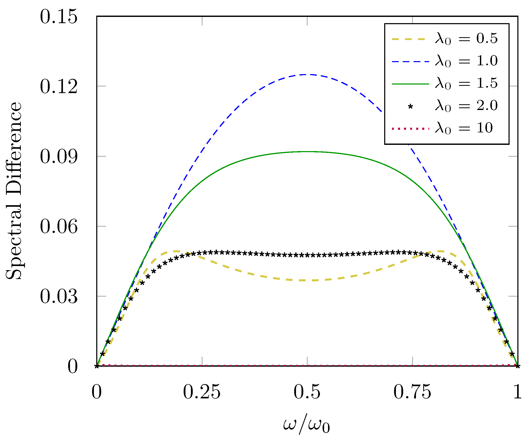
One can see that the spectral ratio and difference for the newly calculated moving asymmetric Robin boundary closely resembles those found in Section 2.2.2 for the time-dependent moving mirror. One sees from Equation (91) that the left half of the mirror always produces a larger number of particles than the right half, excluding the points and where the spectrum vanishes. This is also apparent in spectral difference, as it is positive for all values outside the end points. As expected, in the Dirichlet limit when the asymmetry vanishes. For a closer look at the difference between spectral outputs by the two sides of the moving asymmetric Robin b.c., including the influence of difference values of ; see Figure 2.
3.2.2. Particle Creation Rate
The total number of particles created, effectively the (average) particle creation rate, is
where with
and
This particle creation rate is the physically meaningful quantity that can be experimentally measured. One can see that is proportional to (a result of the open geometry of the cavity). The particle creation rate in the limits of (Dirichlet) and (Neumann) converge to the same value:
which matches what is found in the literature [23,26,37].
4. Comparison between the Different Approaches
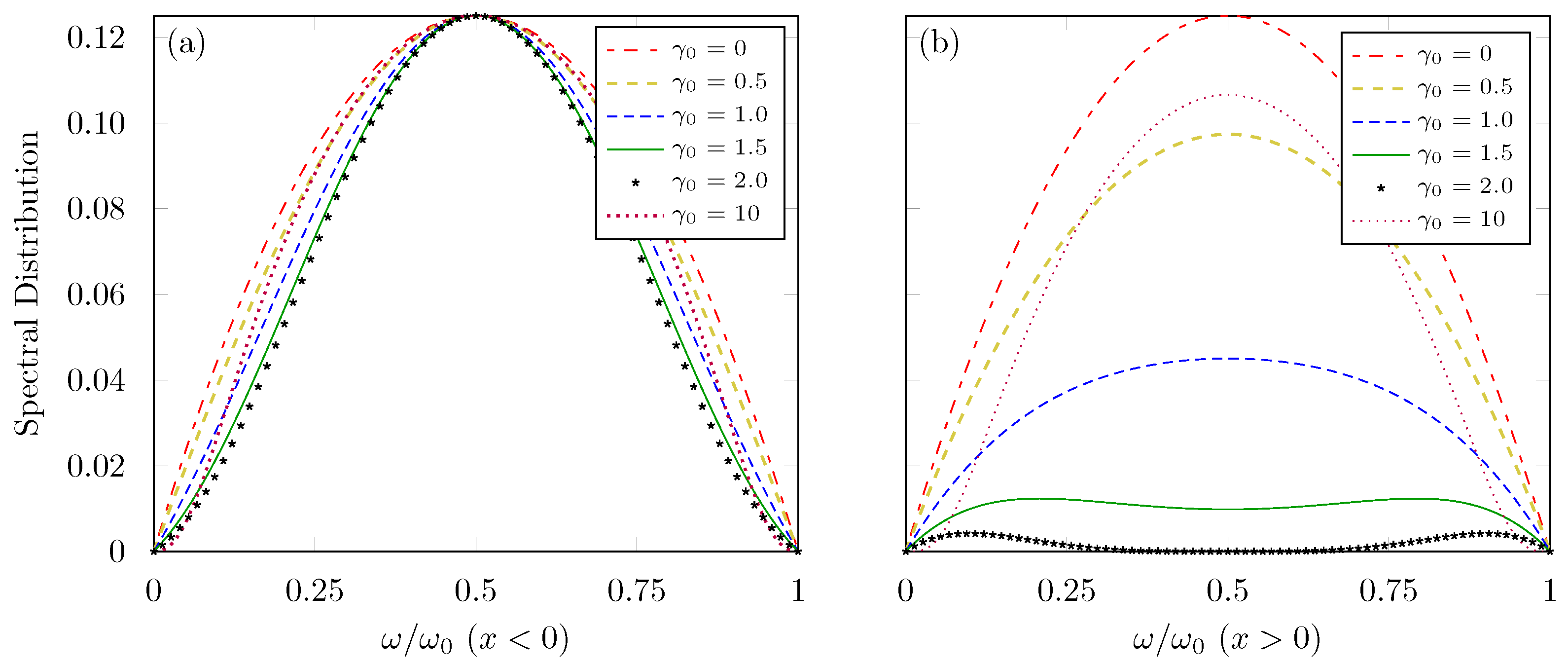
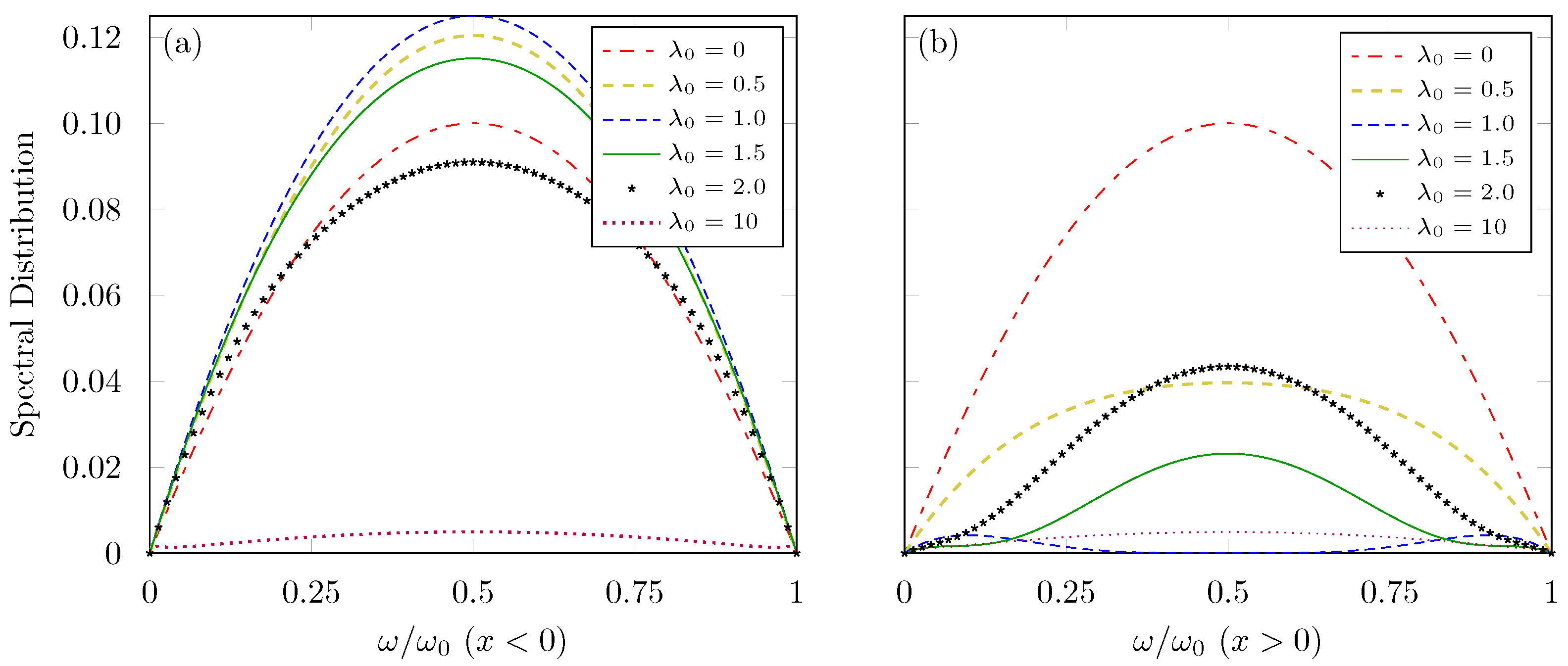
The moving asymmetric Robin boundary solution that we constructed in Section 3.2 bears a striking resemblance to the moving mirror that originates from the scattering approach. One can examine the two solutions alongside each other by looking at their respective spectral distributions in Figure 2 and Figure 3. For the sake of comparison, let us consider the maximally asymmetric cases for the different solutions, which correspond to and (taking with ). The spectrum , on right side of the mirror, is the same as both the original unperturbed moving Robin b.c. spectrum [79] and the spectrum produced by the right side of the moving mirror [46]. This Robin spectrum, in Figure 2b, is associated with the highest degree of asymmetry as it is maximally suppressed when (or ), with the spectrum completely vanishing at . From Figure 2a and Figure 3a, the spectrum produced by the left half, , is a purely reflective Dirichlet spectrum when and for the moving and asymmetric Robin mirror, respectively. However, in the maximally asymmetric case of the moving asymmetric Robin mirror, when , there is an inhibition of modes away from that sharpens the purely reflective Dirichlet peak and leaves the maximum value at unchanged.
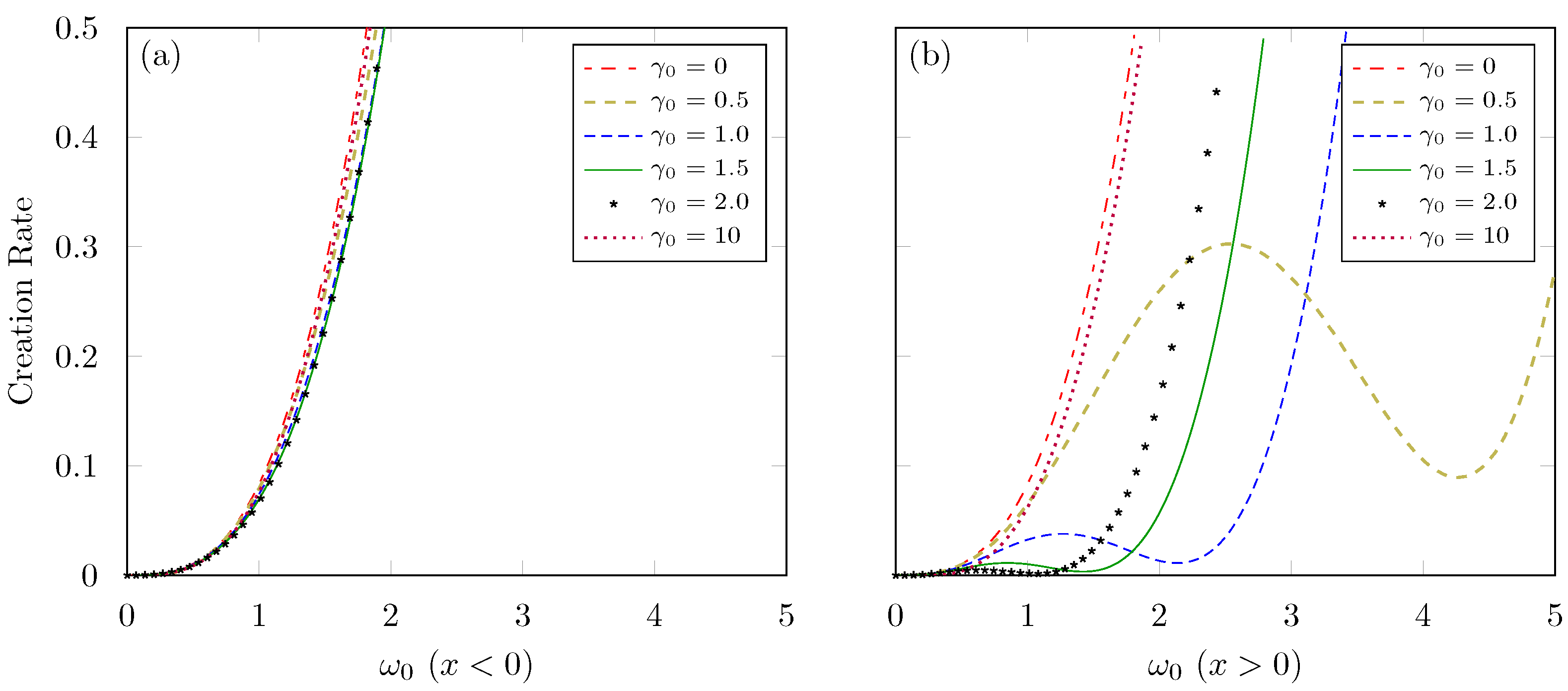
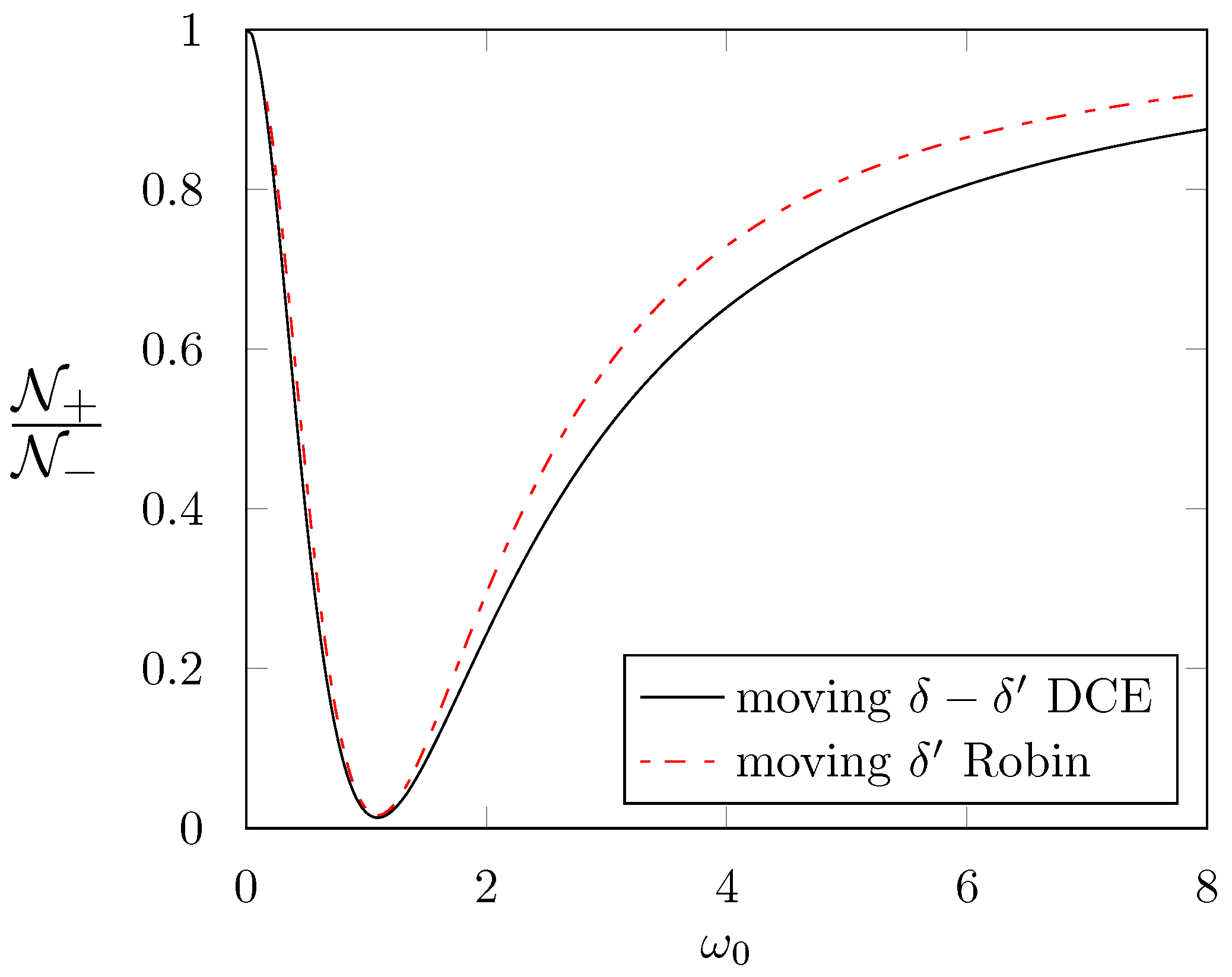
The slight inhibition of modes away from in the maximally asymmetric case of the moving asymmetric Robin b.c. solution, seen in Figure 4b, is what leads to the difference between the particle production ratio of the asymmetric Robin and mirrors. This is well seen in the increased asymmetry in the solution for different values of when compared to the asymmetric Robin solution. Particle production is maximally suppressed for , the frequency of maximal asymmetric particle production, which gives rise to approximately the same minimum in the particle creation ratios seen in Figure 5. Both minima occur at , where for the asymmetric Robin and for the mirrors. From another view, the left side produces about 60 and 75 times that of the right side, respectively.
5. Discussion
The means by which macroscopic systems interacting with the quantum vacuum are able to produce the ADCE are apparent; it is necessary to generate solutions that include both fluctuations in time and explicitly broken spatially symmetry. Without fluctuations in time, be it on the object’s position, material properties, etc., the production of particles vanishes. Unless asymmetric boundary conditions are imposed on either side of an object in (1+1)D, the production of particles will always be symmetric about the two sides of the object and the ADCE will not exist. The appearance of the ADCE is independent of the method used to generate the boundary that interacts with the vacuum. Whether an asymmetric system is solved in a waves-based scattering interaction framework or with a particle-based calculation of the creation/annihilation operators, the same asymmetric effect is present in the solutions of these two approaches. This is especially evident in our newly constructed moving asymmetric Robin b.c. solution, where the introduction of spatial asymmetry to an otherwise symmetric mirror obeying the Robin b.c. induced a change in the particle output of one side of the mirror.
One of the more remarkable consequences of the ADCE is that the unbalanced production of particles will cause an otherwise stationary system to be perturbed via its interaction with the vacuum and induce motion as momentum is “extracted” from the vacuum [47]. The initial state of the object, for (), is that of a stationary, time-independent object interacting with a field. It is completely described by the quantum vacuum state as there are no quantum interactions before the time fluctuations occur. The characteristic oscillations of the time-dependent boundary begin at , i.e., some generic variable of the system , after which the object is free to move. Note that, once the object is able to move, the quantum field will cause the object to experience Brownian motion [86,87,88,89]. Assuming the object is large enough, this motion can be neglected. At this point, if the object possesses no spatial asymmetry while undergoing time fluctuations, the object remains in its starting position as the symmetric production of particles applies an equal and opposite response to the object. For an asymmetric object, particle production is favored to one side, which results in a net force on the object, a transfer of momentum to the previously stationary system, and a dissipation of energy from the mirror. This is expected from the underlying symmetries of quantum field theory (translational invariance, locality, and unitarity). A nonzero vacuum momentum, and a nonvanishing total force, are to be found in any asymmetrically excited system [90].
The total energy of the created particles, , is the sum of the two sides where . The momentum is now , where . The quantity that determines the asymmetric dynamics is , as one now has and . If the system is closed, the energy of the particles emitted comes at the expense of the internal energy of the object, as energy is needed to drive the time fluctuations, and the mass of the object will now change in time. To ensure the total momentum of the system is conserved, the object experiences a net force and now has a nonzero final momentum since the total momentum of the particles no longer vanishes for asymmetric objects. For a detailed analysis of the forces and dynamical evolution of an asymmetric object with time-dependent material properties interacting with the vacuum, see [47]. Here, it is necessary to not only include the motional contribution from the vacuum’s interaction with the time-dependent properties of object, but also the interaction due to its newly perturbed fluctuation in position. Thus, to perform a detailed analysis of the motional corrective terms introduced in [47], one must account for the interaction term between the time dependence on and the position in the example that was explored in Section 2 (see [91] for this process conducted on a symmetric Robin boundary). Accounting for every form of time fluctuations is necessary to understand the full dynamics of the system, an analysis we intend to perform in the future.
Understanding the fundamental mechanisms of asymmetric vacuum interactions provides the basis to investigate an abundance of vacuum interactions that seek to probe the extreme limits of physical theory. Already, we have seen an otherwise stationary object gain momentum out of seemingly nothing, due to its interaction with the vacuum, a surprising result that actually arises from the conservation of momentum. This is not the only time that asymmetric systems have gained momentum from vacuum interactions. It has been shown that a net transfer of linear momentum can occur in a system composed of two excited, dissimilar atoms [90]. Just as it was seen throughout this paper, a quantum system with asymmetric excitations leads to an imbalanced production of emitted particles and gives rise to a net force and transfer of momentum from the vacuum. Linear asymmetry is not the only means by which to generate some motive force from the vacuum: chiral particles can also achieve a similar effect. These particles, which do not posses mirror invariance, can gain kinetic “Casimir” momentum when subjected to a magnetic field [92,93]. There are claims, albeit controversial [94,95,96,97], that the vacuum can impart momentum asymmetrically on magnetoelectric materials [94]. Asymmetric momentum transfer is said to arise from the magnetoelectric molecular structure, as it possesses optical anisotropy since the structure breaks the temporal and spatial symmetries of electromagnetic modes. Even though the details still need to be fully worked out, it is clear that asymmetric vacuum interactions play a role in understanding magnetoelectric and other anistropic materials.
6. Conclusions
We reviewed past studies on the mirror and showed that, regardless of the mechanism and form of the time-dependent fluctuations, the ADCE is produced. Fluctuations on were explored and we discussed obstructions to analyzing linear scattering in this case. Experimental motivations were discussed. We showed, in the scattering framework, that physically relevant quantities originate purely from the difference between right- and left-half asymmetric transmission and reflection coefficients. A newly formulated solution using the Bogoliubov transform introduces an asymmetric formulation of the moving Robin boundary. This solution bears a striking resemblance to the moving mirror, demonstrating the ability to break symmetric boundary solutions and build up new forms of ADCE configurations. Byproducts of the ADCE were explored, namely the transfer of momentum to otherwise stationary systems, causing an object to move through the vacuum without any addition external forces beyond the vacuum interactions. Remarkably, momentum transfer here emerges from the enforcement of conservation laws, not a violation of them.
Within the framework of objects interacting in (1+1)D with the massless scalar quantum field, we have explored the effects of introducing asymmetry to time-dependent systems interacting with the quantum vacuum and demonstrated general consequences that asymmetric boundary conditions impart upon these systems. Whether the problem is approached from the perspective of quantum particles or quantum fields, the end result is the same: an asymmetric production of photons between the two sides of an object. An explicit breaking of mirror symmetry about the two sides of an object is necessary to generate the asymmetry needed to produce different spectra and quantities of particles about the two sides of the object. Additionally, without time-dependent fluctuations of object–vacuum interactions the particle production vanishes. It is necessary to have perturbations on both the spatial and temporal domains of the system to break the underlying symmetry of vacuum interactions.
Author Contributions
Conceptualization, M.J.G.; methodology, M.J.G.; software, M.J.G. and W.D.J.; validation, M.J.G., W.D.J., P.M.B. and J.A.M.; formal analysis, M.J.G., W.D.J., P.M.B. and J.A.M.; investigation, M.J.G. and W.D.J.; resources, G.B.C.; data curation, M.J.G. and W.D.J.; writing—original draft preparation, M.J.G. and W.D.J.; writing—review and editing, P.M.B., J.A.M. and G.B.C.; supervision, G.B.C.; project administration, G.B.C. All authors have read and agreed to the published version of the manuscript.
Funding
This research received no external funding.
Data Availability Statement
Not applicable.
Acknowledgments
The authors would like to thank Ramesh Radhakrishnan, Cooper Watson, and Eric Davis for beneficial discussions and reviews. The authors would also like to thank the reviewers.
Conflicts of Interest
The authors declare no conflict of interest.
Abbreviations
The following abbreviations are used in this manuscript:
| ADCE | asymmetric dynamical Casimir effect |
| b.c. | boundary condition |
| D | dimension |
| DCE | dynamical Casimir effect |
| SQUID | superconducting quantum interference device |
Appendix A. λ(t) Linear Scattering
Here, we provide a derivation of the scattering terms for chosen such that the resulting expressions for matching conditions are as simple as possible. This allows us straightforward illustration of the way in which we are obstructed from deriving scattering matrix elements as we did in the rest of this paper.
Starting from Equations (61) and (62),
and
it becomes seen that a general form of the matching conditions cannot be derived due to convolution Fourier transforms. To demonstrate the difficulty these integrals provide for the matching conditions, we take specific form , where f is assumed for now to have the same type of functional dependence found in Equation (34). We note, though, that we do not specify an explicit functional definition for f. Instead, making the general assumption that in the limit where , one has a “monochromatic-like” limit where its Fourier transform satisfies
where b is some normalization constant for the Dirac delta distributions. Using this, one then has the Fourier transform of as
where in what follows we assume we already computed the limit on whenever evaluating integrals.
Substituting into Equations (61) and (62), one has:
and
Now, explicitly evaluating these integrals under the above limits and assumptions, one obtains:
and
Next, we further assume that the ingoing and outgoing fields are linearly related as before, giving
and
Now, Equations (A5) and (A6) can be re-expressed explicitly in terms of transmission and reflection coefficients, offering
- :
- :
Equations (A7)–(A10) provide four coupled equations, with 12 unknown terms: four scattering terms for each frequency argument appearing (, ). Therefore, there are not enough constraints on the fields to produce a definitive solution to the perturbation for the (1 + 1)D mirror in this scattering approach. The authors are not aware of any technique within this linear scattering framework that would allow for one to solve problems of this type. Additionally, this result seems to suggest that there may be some general obstruction that prevents this type of linear scattering framework from solution when the potential contains a potential with time-dependent strength. This is because potentials in this form typically couple different frequencies together in a way that prevents the matching conditions from being solvable. The authors are still optimistic than an approach based upon Bogoliubov transformations may be more successful, but such an approach requires substantial development which is reserved for future work.
References
- Casimir, H.B.G. On the attraction between two perfectly conducting plates. Proc. Kon. Ned. Akad. Wetensch. 1948, 51, 793–795. Available online: https://dwc.knaw.nl/DL/publications/PU00018547.pdf (accessed on 11 March 2023).
- Milton, K.A. The Casimir Effect: Physical Manifestations of Zero-Point Energy; World Scientific Publishing Co. Pte. Ltd.: Singapore, 2001. [Google Scholar] [CrossRef]
- Milonni, P.W.; Shih, M.L. Casimir forces. Contemp. Phys. 1992, 33, 313–322. [Google Scholar] [CrossRef]
- Milton, K.A. The Casimir effect: Recent controversies and progress. J. Phys. Math. Gen. 2004, 37, R209–R277. [Google Scholar] [CrossRef]
- Lamoreaux, S.K. The Casimir force: Background, experiments, and applications. Rep. Prog. Phys. 2004, 68, 201–236. [Google Scholar] [CrossRef]
- Bordag, M.; Klimchitskaya, G.L.; Mohideen, U.; Mostepanenko, V.M. Advances in the Casimir Effect; Oxford University Press: Oxford, UK, 2009. [Google Scholar] [CrossRef]
- Simpson, W.M.; Leonhardt, U.; Simpson, W.M. Forces of the Quantum Vacuum; World Scientific Publishing Co. Pte. Ltd.: Singapore, 2015. [Google Scholar] [CrossRef]
- Palasantzas, G.; Dalvit, D.A.; Decca, R.; Svetovoy, V.B.; Lambrecht, A. Casimir Physics. J. Phys. Condens. Matter 2015, 27, 210301. [Google Scholar] [CrossRef]
- Moore, G.T. Quantum theory of the electromagnetic field in a variable-length one-dimensional cavity. J. Math. Phys. 1970, 11, 2679–2691. [Google Scholar] [CrossRef]
- DeWitt, B.S. Quantum field theory in curved spacetime. Phys. Rep. 1975, 19, 295–357. [Google Scholar] [CrossRef]
- Fulling, S.A.; Davies, P.C. Radiation from a moving mirror in two dimensional space-time: Conformal anomaly. Proc. R. Soc. Lond. Math. Phys. Sci. 1976, 348, 393–414. [Google Scholar] [CrossRef]
- Davies, P.C.; Fulling, S.A. Radiation from moving mirrors and from black holes. Proc. R. Soc. Lond. Math. Phys. Sci. 1977, 356, 237–257. [Google Scholar] [CrossRef]
- Yablonovitch, E. Accelerating reference frame for electromagnetic waves in a rapidly growing plasma: Unruh-Davies-Fulling-DeWitt radiation and the nonadiabatic Casimir effect. Phys. Rev. Lett. 1989, 62, 1742. [Google Scholar] [CrossRef]
- Dodonov, V. Dynamical Casimir effect: Some theoretical aspects. J. Phys. Conf. Ser. 2009, 161, 012027. [Google Scholar] [CrossRef]
- Dodonov, V. Current status of the dynamical Casimir effect. Phys. Scr. 2010, 82, 038105. [Google Scholar] [CrossRef]
- Dodonov, V. Fifty years of the dynamical Casimir effect. Physics 2020, 2, 67–104. [Google Scholar] [CrossRef]
- Maia Neto, P.A. The dynamical Casimir effect with cylindrical waveguides. J. Opt. B Quantum Semiclass. Opt. 2005, 7, S86–S88. [Google Scholar] [CrossRef]
- Mundarain, D.F.; Maia Neto, P.A. Quantum radiation in a plane cavity with moving mirrors. Phys. Rev. A 1998, 57, 1379–1390. [Google Scholar] [CrossRef]
- Eberlein, C. Sonoluminescence as quantum vacuum radiation. Phys. Rev. Lett. 1996, 76, 3842–3845. [Google Scholar] [CrossRef]
- Crocce, M.; Dalvit, D.A.; Lombardo, F.C.; Mazzitelli, F.D. Hertz potentials approach to the dynamical Casimir effect in cylindrical cavities of arbitrary section. J. Opt. B Quantum Semiclass. Opt. 2005, 7, S32–S39. [Google Scholar] [CrossRef]
- Crocce, M.; Dalvit, D.A.; Mazzitelli, F.D. Resonant photon creation in a three-dimensional oscillating cavity. Phys. Rev. A 2001, 64, 013808. [Google Scholar] [CrossRef]
- Dodonov, V.V.; Klimov, A.B. Generation and detection of photons in a cavity with a resonantly oscillating boundary. Phys. Rev. A 1996, 53, 2664–2682. [Google Scholar] [CrossRef]
- Alves, D.T.; Farina, C.; Maia Neto, P.A. Dynamical Casimir effect with Dirichlet and Neumann boundary conditions. J. Phys. A Math. Gen. 2003, 36, 11333–11342. [Google Scholar] [CrossRef]
- Alves, D.T.; Farina, C.; Granhen, E.R. Dynamical Casimir effect in a resonant cavity with mixed boundary conditions. Phys. Rev. A 2006, 73, 063818. [Google Scholar] [CrossRef]
- Alves, D.T.; Granhen, E.R. Energy density and particle creation inside an oscillating cavity with mixed boundary conditions. Phys. Rev. A 2008, 77, 015808. [Google Scholar] [CrossRef]
- Alves, D.T.; Granhen, E.R.; Lima, M.G. Quantum radiation force on a moving mirror with Dirichlet and Neumann boundary conditions for a vacuum, finite temperature, and a coherent state. Phys. Rev. D 2008, 77, 125001. [Google Scholar] [CrossRef]
- Alves, D.T.; Granhen, E.R.; Silva, H.O.; Lima, M.G. Exact behavior of the energy density inside a one-dimensional oscillating cavity with a thermal state. Phys. Lett. A 2010, 374, 3899–3907. [Google Scholar] [CrossRef]
- Good, M.R.R.; Anderson, P.R.; Evans, C.R. Mirror reflections of a black hole. Phys. Rev. D 2016, 94, 065010. [Google Scholar] [CrossRef]
- Good, M.R.R.; Zhakenuly, A.; Linder, E.V. Mirror at the edge of the universe: Reflections on an accelerated boundary correspondence with de Sitter cosmology. Phys. Rev. D 2020, 102, 045020. [Google Scholar] [CrossRef]
- Good, M.R.R.; Lapponi, A.; Luongo, O.; Mancini, S. Quantum communication through a partially reflecting accelerating mirror. Phys. Rev. D 2021, 104, 105020. [Google Scholar] [CrossRef]
- Haro, J.; Elizalde, E. Hamiltonian approach to the dynamical Casimir effect. Phys. Rev. Lett. 2006, 97, 130401. [Google Scholar] [CrossRef]
- Haro, J.; Elizalde, E. Physically sound Hamiltonian formulation of the dynamical Casimir effect. Phys. Rev. D 2007, 76, 065001. [Google Scholar] [CrossRef]
- Jackel, M.-T.; Reynaud, S. Fluctuations and dissipation for a mirror in vacuum. Quantum Opt. J. Eur. Opt. Soc. Part B 1992, 4, 39–53. [Google Scholar] [CrossRef]
- Barton, G.; Eberlein, C. On quantum radiation from a moving body with finite refractive index. Ann. Phys. 1993, 227, 222–274. [Google Scholar] [CrossRef]
- Barton, G.; Calogeracos, A. On the quantum electrodynamics of a dispersive mirror. I. Mass shifts, radiation, and radiative reaction. Ann. Phys. 1995, 238, 227–267. [Google Scholar] [CrossRef]
- Barton, G.; Calogeracos, A. On the quantum electrodynamics of a dispersive mirror. II. The Boundary condition and the applied force via Dirac’s theory of constraints. Ann. Phys. 1995, 238, 268–285. [Google Scholar] [CrossRef]
- Lambrecht, A.; Jaekel, M.-T.; Reynaud, S. Motion induced radiation from a vibrating cavity. Phys. Rev. Lett. 1996, 77, 615–618. [Google Scholar] [CrossRef] [PubMed]
- Obadia, N.; Parentani, R. Notes on moving mirrors. Phys. Rev. D 2001, 64, 044019. [Google Scholar] [CrossRef]
- Nicolaevici, N. Quantum radiation from a partially reflecting moving mirror. Class. Quant. Grav. 2001, 18, 619–628. [Google Scholar] [CrossRef]
- Haro, J.; Elizalde, E. Black hole collapse simulated by vacuum fluctuations with a moving semitransparent mirror. Phys. Rev. D 2008, 77, 045011. [Google Scholar] [CrossRef]
- Nicolaevici, N. Semitransparency effects in the moving mirror model for Hawking radiation. Phys. Rev. D 2009, 80, 125003. [Google Scholar] [CrossRef]
- Fosco, C.D.; Giraldo, A.; Mazzitelli, F.D. Dynamical Casimir effect for semitransparent mirrors. Phys. Rev. D 2017, 96, 045004. [Google Scholar] [CrossRef]
- Dalvit, D.A.R.; Maia Neto, P.A. Decoherence via the dynamical Casimir effect. Phys. Rev. Lett. 2000, 84, 798–801. [Google Scholar] [CrossRef]
- Muñoz-Castañeda, J.M.; Guilarte, J.M. δ-δ′ generalized Robin boundary conditions and quantum vacuum fluctuations. Phys. Rev. D 2015, 91, 025028. [Google Scholar] [CrossRef]
- Braga, A.N.; Silva, J.D.L.; Alves, D.T. Casimir force between δ-δ′ mirrors transparent at high frequencies. Phys. Rev. D 2016, 94, 125007. [Google Scholar] [CrossRef]
- Silva, J.D.L.; Braga, A.N.; Alves, D.T. Dynamical Casimir effect with δ-δ′ mirrors. Phys. Rev. D 2016, 94, 105009. [Google Scholar] [CrossRef]
- Silva, J.D.L.; Braga, A.N.; Rego, A.L.; Alves, D.T. Motion induced by asymmetric excitation of the quantum vacuum. Phys. Rev. D 2020, 102, 125019. [Google Scholar] [CrossRef]
- Rego, A.L.; Braga, A.N.; Silva, J.D.L.; Alves, D.T. Dynamical Casimir effect enhanced by decreasing the mirror reflectivity. Phys. Rev. D 2022, 105, 025013. [Google Scholar] [CrossRef]
- Jaekel, M.T.; Reynaud, S. Casimir force between partially transmitting mirrors. J. Phys. I 1991, 1, 1395–1409. [Google Scholar] [CrossRef]
- Maghrebi, M.F.; Golestanian, R.; Kardar, M. Scattering approach to the dynamical Casimir effect. Phys. Rev. D 2013, 87, 025016. [Google Scholar] [CrossRef]
- Kurasov, P.B.; Scrinzi, A.; Elander, N. δ′ potential arising in exterior complex scaling. Phys. Rev. A 1994, 49, 5095–5097. [Google Scholar] [CrossRef]
- Kurasov, P. Distribution theory for discontinuous test functions and differential operators with generalized coefficients. J. Math. Anal. Appl. 1996, 201, 297–323. [Google Scholar] [CrossRef]
- Gadella, M.; Negro, J.; Nieto, L. Bound states and scattering coefficients of the- aδ(x) + bδ′(x) potential. Phys. Lett. A 2009, 373, 1310–1313. [Google Scholar] [CrossRef]
- Kim, W.J.; Brownell, J.H.; Onofrio, R. Detectability of dissipative motion in quantum vacuum via superradiance. Phys. Rev. Lett. 2006, 96, 200402. [Google Scholar] [CrossRef] [PubMed]
- Brownell, J.H.; Kim, W.J.; Onofrio, R. Modelling superradiant amplification of Casimir photons in very low dissipation cavities. J. Phys. A Math. Theor. 2008, 41, 164026. [Google Scholar] [CrossRef]
- Motazedifard, A.; Dalafi, A.; Naderi, M.; Roknizadeh, R. Controllable generation of photons and phonons in a coupled Bose–Einstein condensate-optomechanical cavity via the parametric dynamical Casimir effect. Ann. Phys. 2018, 396, 202–219. [Google Scholar] [CrossRef]
- Sanz, M.; Wieczorek, W.; Gröblacher, S.; Solano, E. Electro-mechanical Casimir effect. Quantum 2018, 2, 91. [Google Scholar] [CrossRef]
- Qin, W.; Macrì, V.; Miranowicz, A.; Savasta, S.; Nori, F. Emission of photon pairs by mechanical stimulation of the squeezed vacuum. Phys. Rev. A 2019, 100, 062501. [Google Scholar] [CrossRef]
- Butera, S.; Carusotto, I. Mechanical backreaction effect of the dynamical Casimir emission. Phys. Rev. A 2019, 99, 053815. [Google Scholar] [CrossRef]
- Nation, P.B.; Johansson, J.R.; Blencowe, M.P.; Nori, F. Colloquium: Stimulating uncertainty: Amplifying the quantum vacuum with superconducting circuits. Rev. Mod. Phys. 2012, 84, 1–24. [Google Scholar] [CrossRef]
- Wilson, C.M.; Johansson, G.; Pourkabirian, A.; Simoen, M.; Johansson, J.R.; Duty, T.; Nori, F.; Delsing, P. Observation of the dynamical Casimir effect in a superconducting circuit. Nature 2011, 479, 376–379. [Google Scholar] [CrossRef] [PubMed]
- Schützhold, R.; Plunien, G.; Soff, G. Quantum radiation in external background fields. Phys. Rev. A 1998, 58, 1783–1793. [Google Scholar] [CrossRef]
- Dodonov, V.V.; Klimov, A.B.; Nikonov, D.E. Quantum phenomena in nonstationary media. Phys. Rev. A 1993, 47, 4422–4429. [Google Scholar] [CrossRef]
- Braggio, C.; Bressi, G.; Carugno, G.; Del Noce, C.; Galeazzi, G.; Lombardi, A.; Palmieri, A.; Ruoso, G.; Zanello, D. A novel experimental approach for the detection of the dynamical Casimir effect. Europhys. Lett. (EPL) 2005, 70, 754–760. [Google Scholar] [CrossRef]
- De Liberato, S.; Ciuti, C.; Carusotto, I. Quantum vacuum radiation spectra from a semiconductor microcavity with a time-modulated vacuum Rabi frequency. Phys. Rev. Lett. 2007, 98, 103602. [Google Scholar] [CrossRef] [PubMed]
- Günter, G.; Anappara, A.A.; Hees, J.; Sell, A.; Biasiol, G.; Sorba, L.; De Liberato, S.; Ciuti, C.; Tredicucci, A.; Leitenstorfer, A.; et al. Sub-cycle switch-on of ultrastrong light–matter interaction. Nature 2009, 458, 178–181. [Google Scholar] [CrossRef]
- Johansson, J.R.; Johansson, G.; Wilson, C.M.; Nori, F. Dynamical Casimir effect in a superconducting coplanar waveguide. Phys. Rev. Lett. 2009, 103, 147003. [Google Scholar] [CrossRef]
- Wilson, C.M.; Duty, T.; Sandberg, M.; Persson, F.; Shumeiko, V.; Delsing, P. Photon generation in an electromagnetic cavity with a time-dependent boundary. Phys. Rev. Lett. 2010, 105, 233907. [Google Scholar] [CrossRef] [PubMed]
- Dezael, F.X.; Lambrecht, A. Analogue Casimir radiation using an optical parametric oscillator. EPL (Europhys. Lett.) 2010, 89, 14001. [Google Scholar] [CrossRef]
- Lähteenmäki, P.; Paraoanu, G.S.; Hassel, J.; Hakonen, P.J. Dynamical Casimir effect in a Josephson metamaterial. Proc. Natl. Acad. Sci. USA 2013, 110, 4234–4238. [Google Scholar] [CrossRef]
- Schneider, B.H.; Bengtsson, A.; Svensson, I.M.; Aref, T.; Johansson, G.; Bylander, J.; Delsing, P. Observation of broadband entanglement in microwave radiation from a single time-varying boundary condition. Phys. Rev. Lett. 2020, 124, 140503. [Google Scholar] [CrossRef]
- Vezzoli, S.; Mussot, A.; Westerberg, N.; Kudlinski, A.; Dinparasti Saleh, H.; Prain, A.; Biancalana, F.; Lantz, E.; Faccio, D. Optical analogue of the dynamical Casimir effect in a dispersion-oscillating fibre. Commun. Phys. 2019, 2, 84. [Google Scholar] [CrossRef]
- Torricelli, G.; van Zwol, P.J.; Shpak, O.; Binns, C.; Palasantzas, G.; Kooi, B.J.; Svetovoy, V.B.; Wuttig, M. Switching Casimir forces with phase-change materials. Phys. Rev. A 2010, 82, 010101. [Google Scholar] [CrossRef]
- Banishev, A.A.; Chang, C.-C.; Castillo-Garza, R.; Klimchitskaya, G.L.; Mostepanenko, V.M.; Mohideen, U. Modifying the Casimir force between indium tin oxide film and Au sphere. Phys. Rev. B 2012, 85, 045436. [Google Scholar] [CrossRef]
- Wegkamp, D.; Stähler, J. Ultrafast dynamics during the photoinduced phase transition in VO2. Prog. Surf. Sci. 2015, 90, 464–502. [Google Scholar] [CrossRef]
- Mogunov, I.A.; Fernández, F.; Lysenko, S.; Kent, A.J.; Scherbakov, A.V.; Kalashnikova, A.M.; Akimov, A.V. Ultrafast insulator-metal transition in VO2 nanostructures assisted by picosecond strain pulses. Phys. Rev. Appl. 2019, 11, 014054. [Google Scholar] [CrossRef]
- Sood, A.; Shen, X.; Shi, Y.; Kumar, S.; Park, S.J.; Zajac, M.; Sun, Y.; Chen, L.-Q.; Ramanathan, S.; Wang, X.; et al. Universal phase dynamics in VO2 switches revealed by ultrafast operando diffraction. Science 2021, 373, 352–355. [Google Scholar] [CrossRef] [PubMed]
- Shabanpour, J.; Beyraghi, S.; Cheldavi, A. Ultrafast reprogrammable multifunctional vanadium-dioxide-assisted metasurface for dynamic THz wavefront engineering. Sci. Rep. 2020, 10, 8950. [Google Scholar] [CrossRef] [PubMed]
- Mintz, B.; Farina, C.; Maia Neto, P.A.; Rodrigues, R.B. Particle creation by a moving boundary with a Robin boundary condition. J. Phys. A Math. Gen. 2006, 39, 11325–11333. [Google Scholar] [CrossRef]
- Mintz, B.; Farina, C.; Maia Neto, P.A.; Rodrigues, R.B. Casimir forces for moving boundaries with Robin conditions. J. Phys. A Math. Gen. 2006, 39, 6559–6565. [Google Scholar] [CrossRef]
- Rego, A.L.; Mintz, B.; Farina, C.; Alves, D.T. Inhibition of the dynamical Casimir effect with Robin boundary conditions. Phys. Rev. D 2013, 87, 045024. [Google Scholar] [CrossRef]
- Ford, L.H.; Vilenkin, A. Quantum radiation by moving mirrors. Phys. Rev. D 1982, 25, 2569–2575. [Google Scholar] [CrossRef]
- Silva, H.O.; Farina, C. Simple model for the dynamical Casimir effect for a static mirror with time-dependent properties. Phys. Rev. D 2011, 84, 045003. [Google Scholar] [CrossRef]
- Mostepanenko, V.M.; Trunov, N.N. Quantum field theory of the Casimir effect for real media. Sov. J. Nucl. Phys. 1985, 42, 818–822. [Google Scholar]
- Farina, C.; Silva, H.O.; Rego, A.L.; Alves, D.T. Time-dependent Robin boundary conditions in the dynamical Casimir effect. Int. J. Mod. Phys. Conf. Ser 2012, 14, 306–315. [Google Scholar] [CrossRef]
- Sinha, S.; Sorkin, R.D. Brownian motion at absolute zero. Phys. Rev. B 1992, 45, 8123–8126. [Google Scholar] [CrossRef] [PubMed]
- Jaekel, M.T.; Reynaud, S. Quantum fluctuations of position of a mirror in vacuum. J. Phys. I France 1993, 3, 1–20. [Google Scholar] [CrossRef]
- Stargen, D.J.; Kothawala, D.; Sriramkumar, L. Moving mirrors and the fluctuation-dissipation theorem. Phys. Rev. D 2016, 94, 025040. [Google Scholar] [CrossRef]
- Wang, Q.; Zhu, Z.; Unruh, W.G. How the huge energy of quantum vacuum gravitates to drive the slow accelerating expansion of the Universe. Phys. Rev. D 2017, 95, 103504. [Google Scholar] [CrossRef]
- Donaire, M. Net force on an asymmetrically excited two-atom system from vacuum fluctuations. Phys. Rev. A 2016, 94, 062701. [Google Scholar] [CrossRef]
- Silva, J.D.L.; Braga, A.N.; Rego, A.L.; Alves, D.T. Interference phenomena in the dynamical Casimir effect for a single mirror with Robin conditions. Phys. Rev. D 2015, 92, 025040. [Google Scholar] [CrossRef]
- Donaire, M.; van Tiggelen, B.; Rikken, G.L.J.A. Casimir momentum of a chiral molecule in a magnetic field. Phys. Rev. Lett. 2013, 111, 143602. [Google Scholar] [CrossRef] [PubMed]
- Donaire, M.; Van Tiggelen, B.A.; Rikken, G.L.J.A. Transfer of linear momentum from the quantum vacuum to a magnetochiral molecule. J. Phys. Cond. Matter 2015, 27, 214002. [Google Scholar] [CrossRef]
- Feigel, A. Quantum vacuum contribution to the momentum of dielectric media. Phys. Rev. Lett. 2004, 92, 020404. [Google Scholar] [CrossRef] [PubMed]
- Croze, O.A. Does the Feigel effect break the first law? arXiv 2013, arXiv:1304.3338. [Google Scholar] [CrossRef]
- Croze, O.A. Alternative derivation of the Feigel effect and call for its experimental verification. Proc. R. Soc. A Math. Phys. Eng. Sci. 2012, 468, 429–447. [Google Scholar] [CrossRef]
- Birkeland, O.J.; Brevik, I. Feigel effect: Extraction of momentum from vacuum? Phys. Rev. E 2007, 76, 066605. [Google Scholar] [CrossRef] [PubMed]
Figure 1.
The plot of , the difference between the spectral distributions of particles created on the two sides of a mirror as a function of for different values of , with . See text for details.
Figure 1.
The plot of , the difference between the spectral distributions of particles created on the two sides of a mirror as a function of for different values of , with . See text for details.

Figure 2.
The spectral distribution of particles created on the two sides of the mirror as a function of for different values of : (a) the plot of ; (b) the plot of . See text for details.
Figure 2.
The spectral distribution of particles created on the two sides of the mirror as a function of for different values of : (a) the plot of ; (b) the plot of . See text for details.

Figure 3.
The spectral distribution of particles created on the two sides of a moving mirror as a function of for different values of , with : (a) the plot of ; (b) the plot of . See text for details. Figure is generated from results within Ref. [46].
Figure 3.
The spectral distribution of particles created on the two sides of a moving mirror as a function of for different values of , with : (a) the plot of ; (b) the plot of . See text for details. Figure is generated from results within Ref. [46].

Figure 4.
The creation rate of particles on the two sides of the mirror as a function of for different values of : (a) the plot of ; (b) the plot of . See text for details.
Figure 4.
The creation rate of particles on the two sides of the mirror as a function of for different values of : (a) the plot of ; (b) the plot of . See text for details.

Figure 5.
The particle creation ratio of for both the moving asymmetric Robin and boundaries. For comparison, the asymmetric Robin mirror with and the mirror with are shown.
Figure 5.
The particle creation ratio of for both the moving asymmetric Robin and boundaries. For comparison, the asymmetric Robin mirror with and the mirror with are shown.

Disclaimer/Publisher’s Note: The statements, opinions and data contained in all publications are solely those of the individual author(s) and contributor(s) and not of MDPI and/or the editor(s). MDPI and/or the editor(s) disclaim responsibility for any injury to people or property resulting from any ideas, methods, instructions or products referred to in the content. |
© 2023 by the authors. Licensee MDPI, Basel, Switzerland. This article is an open access article distributed under the terms and conditions of the Creative Commons Attribution (CC BY) license (https://creativecommons.org/licenses/by/4.0/).
Share and Cite
MDPI and ACS Style
Gorban, M.J.; Julius, W.D.; Brown, P.M.; Matulevich, J.A.; Cleaver, G.B. The Asymmetric Dynamical Casimir Effect. Physics 2023, 5, 398-422. https://doi.org/10.3390/physics5020029
AMA Style
Gorban MJ, Julius WD, Brown PM, Matulevich JA, Cleaver GB. The Asymmetric Dynamical Casimir Effect. Physics. 2023; 5(2):398-422. https://doi.org/10.3390/physics5020029
Chicago/Turabian StyleGorban, Matthew J., William D. Julius, Patrick M. Brown, Jacob A. Matulevich, and Gerald B. Cleaver. 2023. "The Asymmetric Dynamical Casimir Effect" Physics 5, no. 2: 398-422. https://doi.org/10.3390/physics5020029