Nonlinear Coupling of Alfvén and Slow Magnetoacoustic Waves in Partially Ionized Solar Plasmas: The Effect of Thermal Misbalance


1
Departament de Física, Universitat Illes Balears, 07122 Palma, Spain
2
Institute of Applied Computing and Community Code (IAC3), Universitat Illes Balears, 07122 Palma, Spain
Physics 2023, 5(2), 331-351; https://doi.org/10.3390/physics5020025
Submission received: 15 January 2023
/
Revised: 3 March 2023
/
Accepted: 4 March 2023
/
Published: 30 March 2023
(This article belongs to the Special Issue A Themed Issue in Honor of Professor Marcel Goossens on the Occasion of His 75th Birthday)
Abstract
:Solar chromosphere and photosphere, as well as solar atmospheric structures, such as prominences and spicules, are made of partially ionized plasmas. Observations have reported the presence of damped or amplified oscillations in these solar plasmas, which have been interpreted in terms of magnetohydrodynamic (MHD) waves. Slow magnetoacoustic waves could be responsible for these oscillations. The present study investigates the temporal behavior of the field-aligned motions that represent slow magnetoacoustic waves excited in a partially ionized prominence plasma by the ponderomotive force. Starting from single-fluid MHD equations, including radiative losses, a heating mechanism and ambipolar diffusion, and using a regular perturbation method, first- and second-order partial differential equations have been derived. By numerically solving second-order equations describing field-aligned motions, the temporal behavior of the longitudinal velocity perturbations is obtained. The damping or amplification of these perturbations can be explained in terms of heating–cooling misbalance, the damping effect due to ambipolar diffusion and the variation of the first adiabatic exponent with temperature and ionization degree.
1. Introduction
Mechanisms based on linear and nonlinear Alfvén waves have been proposed, in order to explain some phenomena observed in different structures of the solar atmosphere. These waves have been the subject of many studies [1,2,3,4,5,6,7], and indirect signatures have been used to confirm their presence in the solar atmosphere. Furthermore, the dissipation of Alfvén waves has also been proposed as a potential mechanism to explain coronal heating.
When large amplitudes are considered, linearly polarized Alfvén waves generate density perturbations and motions along the magnetic field lines [8,9,10,11]. In most studies related to Alfvén waves, fully ionized ideal plasmas are usually considered and treated as a single fluid. However, plasma is partially ionized in some layers of the solar atmosphere, such as the chromosphere and photosphere, and in solar atmospheric structures, such as prominences and spicules. Consequently, studies of Alfvén waves in partially ionized plasmas have been developed [12,13,14,15,16,17,18,19]. Furthermore, consideration of dissipative effects is of great interest, and must be included, to fully understand the behavior of nonlinear Alfvén waves in partially ionized plasmas. In this sense, the single-fluid approach has been used to study the temporal behavior of nonlinear Alfvén waves in a partially ionized prominence plasma [20]. In this study, ambipolar diffusion, radiative losses and thermal conduction as dissipative mechanisms, together with a constant heating-per-unit volume, were taken into account. Then, the damping of the field-aligned motions and the density perturbations excited in the plasma by the ponderomotive force were studied.
Recently, when studying the damping/amplification of coronal slow waves, thermal misbalance has been considered [21,22,23,24,25,26,27,28,29,30]: this effect of thermal misbalance comes from the fact that when compressive waves are considered, they produce a change in the background thermal equilibrium, because they perturb local thermodynamic parameters—such as density, temperature, etc.—driving a local heating–cooling misbalance. At the same time, feedback between the plasma and the wave appears, and the wave loses or gains energy from the plasma, leading to either wave damping or amplification. Finally, the heating mechanisms considered in the above mentioned studies depend on density, , temperature, T, and the magnetic field, B; therefore, the heating, H, has been expressed as , in which a, b and c have been taken as free parameters, and h is a constant (see [31] for a recent review). Further studies on this topic, related to coronal structures, have been conducted in Refs. [21,22,23,24,25,26,27,28,29,30].
Regarding partially ionized prominence plasmas, this approach was taken into account in Ref. [32], which considered single-fluid equations and a partially ionized hydrogen plasma, in which different radiative losses as well as ambipolar diffusion were taken into account. Then, the temporal behaviors of the linear slow magnetoacoustic waves, propagating parallel to the magnetic field, and of thermal waves were studied. The assumed heating mechanisms were density- and temperature-dependent, and it was shown that for some dependences, slow waves could be amplified. Furthermore, the effect of the temperature- and ionization-degree-dependence of the adiabatic coefficient, , in a partially ionized hydrogen plasma [33] was also considered. However, in the dispersion relation obtained from the linear analysis, and when parallel propagation was considered, ambipolar diffusion only influenced Alfvén waves, but not slow waves, which were only affected by radiative losses and heating; therefore, these thermal mechanisms became responsible for the damping/amplification of the oscillations. Then, the only effects related to partial ionization that affected the temporal behavior of the slow waves were the variation of the numerical value of the adiabatic coefficient with the ionization degree, when different temperatures were considered, and the modification of the sound speed. Consequently, to consider the effects on slow waves propagating parallel to the magnetic field, due to radiative losses, heating mechanisms and ambipolar diffusion, we needed to resort to the nonlinear coupling of Alfvén and slow waves [20], which gives place to field-aligned motions induced by the ponderomotive force. Using a regular perturbation approach, the obtained second order equations included an energy equation involving thermal mechanisms, and a term in which Cowling’s diffusivity, , appeared explicitly. Then, this scheme allowed us to study the temporal behavior of field-aligned velocity perturbations, representing slow magnetoacoustic waves, in a partially ionized plasma influenced by thermal mechanisms and ambipolar diffusion.
On the other hand, in the case of prominence plasmas, radiative equilibrium prominence models, constructed from a balance between incident radiation and cooling [34,35,36], as well as differential emission measures, have demonstrated that a further unknown heating is required, in order to reproduce the observed temperatures in the prominence cores [36,37,38]), and to balance the radiative losses [39,40]. Therefore, it would be interesting to consider prominence heating, characterized by different values of the exponents a and b, describing the temperature and density dependence of the heating mechanism, and to study the effect on the oscillatory processes in prominence plasmas caused by slow waves.
The main aim of this study is to investigate the temporal behavior of the field-aligned motions representing slow magnetoacoustic waves excited by the ponderomotive force in an unbounded partially ionized plasma, with physical properties akin to those of solar prominences, when heating–cooling misbalance and the damping effect due to ambipolar diffusion were present. The present study closely follows [20] using the same background model and dissipative mechanisms. However, some important differences, with respect to Ref. [20], are introduced to the present study: first, apart from ambipolar diffusion, the case of thermal misbalance is considered, and the temporal behavior of slow magnetoacoustic waves is studied, paying attention to the damping/amplification of these waves; second, due to the uncertainty of prominence heating, the calculations consider a general heating term such as , taking a and b as free parameters; third, the thermodynamics of partially ionized gas [41] differ from those of fully ionized or fully neutral gas, and the consideration of a constant value for the adiabatic coefficient, , would overestimate the gas temperature [33]; therefore, in this study three different cases are considered. Initially, and for comparison, a constant is considered; then, the first adiabatic exponent, , is computed under non-local thermodynamic equilibrium (NLTE) and local thermodynamic equilibrium (LTE) conditions [33], whose numerical values depend on density, temperature and ionization degree. Furthermore, a comparison between Hildner [42] and CHIANTI7 [43,44,45] radiative functions was also included.
The layout of the paper is as follows. The background model, ionization state, dissipative mechanisms, methods and resulting equations used for the computations are the same as in Ref. [20], and are summarized in Section 2. Next, in Section 3, considering , second-order equations are solved when thermal misbalance and different heating mechanisms are considered. Then, in Section 3 and Section 4, similar calculations are conducted, considering the first adiabatic exponent, , computed under NLTE and LTE conditions as well as different radiative functions. Section 5 briefly discusses the results.
2. Method and Basic Equations
In what follows here, the theoretical background, on which the obtained results are based, is summarized.
2.1. Background Model
The chemical composition of the prominence plasma here is the same as that considered by [38], the abundance of which is hydrogen and helium, which is fully neutral. The equation of state is
where is the Boltzmann constant, H the atomic mass unit, and i is the ionization degree. The ionization degree of the mixture considered is computed by making use of tables of the ionization degree for different temperatures and pressures in prominence slabs provided in Ref. [38], and which were based on 1D non-LTE radiative transfer models [46]. A polynomial fit to these tables, up to third order in pressure, p, temperature, T, together with product terms or interactions was performed, which allows us to compute the ionization degree for any combination of pressure and temperature. For the rest of the parameters, the values for the magnetic field, density and temperature are those typical of quiescent prominences, respectively: T, oriented along the -axis, , considered constant in the calculations here, while the considered temperature, T, is in the interval of 4000–12,000 K.
Single-fluid equations constituted our starting set of equations, with ambipolar diffusion, radiative losses and heating included, while thermal conduction is neglected, because under prominence conditions thermal conduction times are much longer than radiative times [20,32]. Furthermore, in order to characterize the radiative losses, two optically thin radiative-loss functions, such as Hildner [42] and CHIANTI7 [43,44,45] ones are considered. The general expression for these radiative functions is;
where and were piecewise functions depending on the temperature, with and for Hildner [42], and and for CHIANTI7 [43,44,45] when prominence temperatures are considered. Furthermore, ambipolar diffusion is computed following [20].
By applying a regular perturbation method, up to order two, to the single-fluid equations for parallel propagating waves, first-order equations representing Alfvén waves, and second-order equations describing longitudinal velocity perturbations along with density, pressure and temperature perturbations are obtained. These first-order and second-order equations are described and solved in the following Subsections.
2.2. First-Order Equations
In order to write down all the equations under study in a dimensionless form, let us introduce the following dimensionless quantities:
where is the Alfvén speed at the equilibrium state, is Cowling’s diffusivity at the equilibrium state—which is related to the ambipolar diffusivity coefficient, , through , where corresponds to Spitzer’s diffusivity, is a characteristic length scale corresponding to half the size of the spatial domain under consideration, and is a time scale. Both scales are related through the equilibrium Alfvén speed, , and hereafter bars are dropped, for the sake of simplicity. Then, the first-order equations are:
These two equations involve the components of and vectors, transverse to the equilibrium magnetic field, and can be appropriately combined into an equation for only. By imposing conditions representing a standing oscillation, with wavelength equal to [20], the solution to the transverse velocity perturbation is
where is the initial velocity, is the real part of the Alfén wave frequency and is the imaginary part. The period and damping time, due to ambipolar diffusion, are given by
Once the expression for the perturbed velocity amplitude is known, the solution for the perturbed magnetic field, , can be obtained by integration, to give
2.3. Second-Order Equations
Following [20], the dimensionless second-order equations are:
where
with being the sound speed at the equilibrium state, and , , the density, pressure and temperature perturbations, respectively. Here, the focus is on the solution that represents the generation of slow magnetoacoustic waves due to the nonlinear coupling with the Alfvén waves. Furthermore, from here on, it is assumed that : that is to consider a low- plasma typical of prominences, where the plasma- is defined as
with the magnetic permittivity.
The heat-loss function, which depends on the local plasma parameters, is denoted by L. Typically, in solar applications the heat-loss function L represents the difference between an arbitrary heat input and a radiative loss function, such as
with describing radiative losses while describes the heat input, with the units of both quantities being W · kg. In the case of an equilibrium with uniform temperature, such as we will consider here, the heat loss function is
where and are density and temperature equilibrium, and the factors , are
and
with T, p and held constant, respectively, in the equilibrium state.
On the other hand, use of the characteristic times of the thermal misbalance is made here as introduced in Refs. [21,22,23,25,47,48], which are
where is the specific heat given by
with the mean molecular weight.
These thermal misbalance characteristic times depend on the heating/cooling mechanisms considered, and on the rates of change of these mechanisms with density and temperature, such as can be seen in Equations (19) and (20). Now, developing Equations (19) and (20), and since
one can write the characteristic times for thermal misbalance, in terms of radiative losses and heating functions, obtaining
and, using the characteristic times and , one can also compute and in dimensionless form:
3. Results
In this study, three different cases are considered. First, although a partially ionized plasma is considered, for comparison, a constant is assumed here, independent of the plasma ionization degree, which has been used in many research works involving partially ionized plasmas. Second, instead of using , the first adiabatic exponent, , and its variation with temperature and ionization degree has been computed from the fitted model described in Section 2, and is defined as NLTE . Third, the study considers the case when is computed using the ionization degree obtained from an LTE model, as had usually been done in other studies. Finally, in order to assess the effect of different radiative losses, Hildner’s [42] and CHIANTI7’s optically thin radiative losses [43,44,45] are considered.
On the other hand, in order to assess the effect of the assumed heating mechanisms, different values for the exponents a and b, which describe the density and temperature dependences, respectively, are used, which modify the characteristic thermal misbalance times, , , keeping unmodified the ambipolar diffusion damping time, . In all the considered cases, Equations (10)–(13) are solved under the following initial and boundary conditions,
3.1. , (Constant Heating per Unit Volume)
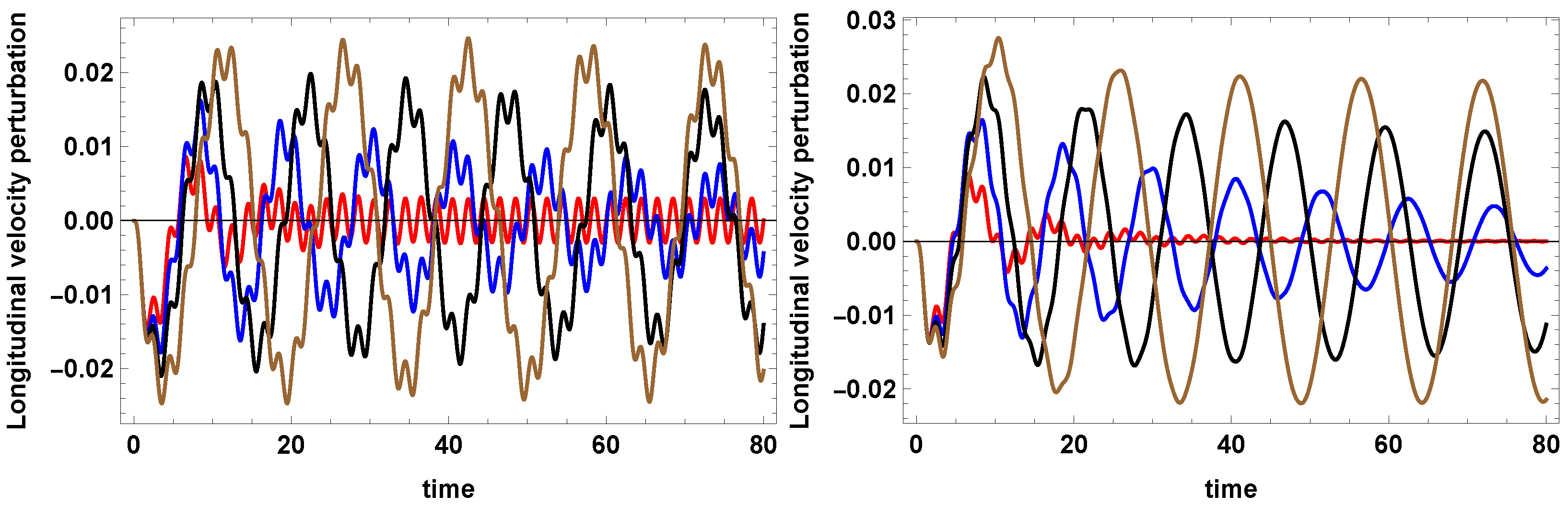
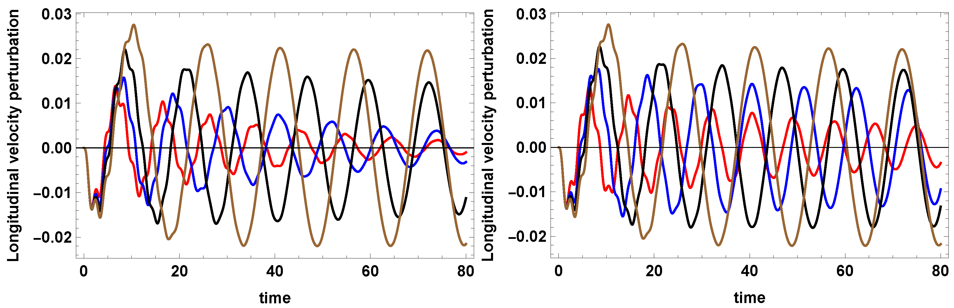
First, and as a reference, let us consider a heating mechanism independent of density and temperature (), which corresponds to a constant heating per unit volume. To describe separately the effects of thermal and ambipolar diffusion, first of all one neglects ambipolar diffusion, and considers only thermal effects. Figure 1 (left) shows, for a characteristic length, m, the dimensionless longitudinal velocity perturbations describing slow waves, corresponding to four different temperatures. The first feature that one can observe in Figure 1 (left) is that the damping produced by radiative losses is different for the different temperatures considered. The stronger damping corresponds to the highest temperature (red curve), while the weaker damping is associated with the lowest temperature (brown curve). Following [32,49], this behavior can be understood by means of the thermal time, , related, in this case, to radiative losses and heating. In the nonlinear case, no analytical expression exists for the thermal damping/amplifying time; however, one can get some help from the linear case [32]. In this case—and assuming small wavenumbers, such as those that are considered in these calculations—the imaginary part of the approximate analytical solution corresponding to slow waves [32] is:
whose sign is given by
Making use, again, of the linear case, the expression describing the damping/amplification due to thermal effects is , and the positive sign of corresponds to the case of time damping, while the negative sign corresponds to amplification. Then, the thermal damping/amplifying time, , can be computed from
becoming
and, as one can see from Equation (31), the thermal time is modified as soon as , , or are modified. Then, using Equation (31): for T = 12,000 K, s; for K, s; for K, s; and for K, s. The numerical values of these thermal times allows us to understand the damping rate of the temporal behavior of the longitudinal velocity perturbations in Figure 1 (left), with the strongest damping corresponding to a temperature, T = 12,000 K, while the weakest damping corresponds to K.
Next, let us consider the effect of ambipolar diffusion and the temporal behavior of longitudinal velocity perturbations, shown in Figure 1 (right). These curves displayed a stronger damping than in Figure 1 (left), due to the inclusion of ambipolar diffusion, whose effect is characterized by (see Equation (6)). In the ambipolar diffusion damping time, introduced in Equation (8), increasing means that the wavenumber is decreased, then is increased, and the effect of ambipolar diffusion becomes weaker; when is decreased, the opposite happens. Keeping constant, a decrease of the temperature means that Cowling’s diffusivity, , is increased, and decreases, which enhances the ambipolar diffusion effect: for T = 12,000 K, s; for K, s; for K, s; and for K, s. For instance, in the curve corresponding to K, one can observe that the damping rate due to thermal effects is very small, because s, while the damping due to ambipolar diffusion ( s) is quite visible at short times; however, in the curve corresponding to T = 12,000 K, and s, which suggests a strong damping due to thermal and ambipolar diffusion effects together, such as can be seen looking at the red curve.
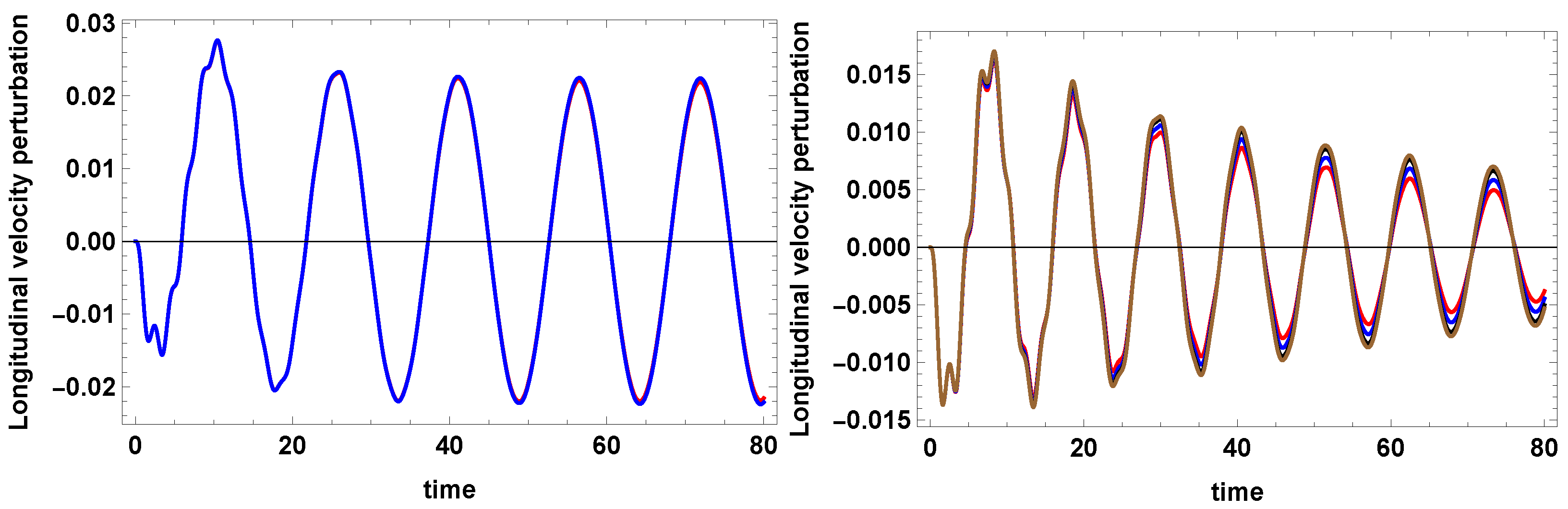
On the other hand, the second characteristic feature of the curves shown in Figure 1 is that the period seems to be increasing when the temperature is decreasing. In order to understand this effect, an analytical approximation is sought. For instance, and as a tentative approximation, one can find from Equations (10)–(13) an analytical solution (shown in Appendix A) for the longitudinal velocity perturbation when thermal effects are neglected. Then, for m and K, this approximate solution is compared to the numerical solution when thermal and ambipolar diffusion effects were taken into account. Figure 2 (left) gives this comparison, and one can observe a good agreement between both solutions because, in this case, ambipolar diffusion is the dominant effect. For different values of and T, when thermal effects become important enough, the agreement is also quite good, with slight differences in the amplitude of both solutions. Consequently, from the analytical solution, one can conclude that the two different frequencies, and (see [8,9,10,11]), are involved in the curves describing the temporal behavior of the oscillations. When temperature is decreased, the sound speed also decreases, and similarly the frequency does; furthermore, decreasing temperature implies an increase in , and, then, the frequency, also decreases. Recapitulating, when the temperature decreases, both frequencies decrease and the period increases, what can be observed in Figure 1 (left) and (right). The temporal behavior of the longitudinal velocity perturbations was dependent on the behavior of , with and with determining damping or amplification, while and determined the period.
Furthermore, to study the damping of MHD waves, optically thin or thick radiative losses, along with different heating mechanisms displaying density and temperature dependence, have been considered by many authors [50,51,52,53]. The assumed values for exponents a and b were: , (constant heating per unit mass); (heating by coronal current dissipation); (heating by Alfvén mode/mode conversion); , (heating by Alfvén mode/anomalous conduction damping). However, taking into account these heating mechanisms, the results always give a damping of the oscillatory processes under study, as one can see in Figure 2 (right). Therefore, it is of great importance to know whether or not damping is a universal behavior independent of the considered heating mechanism. Finally, most of the conclusions obtained, when considering a heating mechanism with , are useful for the studies described in the following Subsections.
3.2. ,
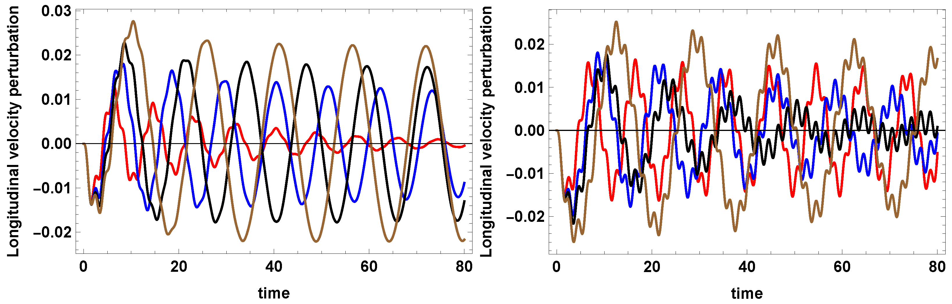
Next, let us consider a heating mechanism that depends on temperature and density, and is characterized by the exponents and . Here, a study similar to that in Section 3.1 is performed, and Figure 3 (left) displays the temporal behavior of the longitudinal velocity perturbations for the same values of temperature, T, and characteristic length, , as in Figure 1. The main difference between Figure 1 and Figure 3 is that the damping proceeds at different rates that can be explained by looking at the thermal times: for T = 12,000 K, s; for K, s; for K, s; for K, = 39,747 s. These thermal times are increased, with respect to those in Section 3.1 because, even though T and are kept constant, the thermal misbalance times, and , are modified, thanks to the new dependence on density and temperature in the heating mechanism. This change in the thermal misbalance times modifies the thermal times, , in Equation (31), while the ambipolar diffusion times stay not modified.
Figure 3 (right) in which the characteristic length, , is increased from m to m, shows a difference in the damping rate, with respect to the Figure 3 (left). There are two reasons explaining the difference. The first reason is that in this case, the effect of the ambipolar diffusion is weaker due to the change in , which produces an increase in the ambipolar diffusion damping times, which are now: T = 12,000 K, = 284,292 s; K, = 246,512 s; K, = 213,772 s; and K, = 174,191 s. One can conclude that to increase by two orders of magnitude produces a substantial increase in . The second reason is that the thermal time also increased, with respect to the case of m. This is also due to the change in the wavenumber, , as it appears in Equation (31), with the thermal times now being: T = 12,000 K, = 360,000 s; K, = 52,279 s; K, = 14,140 s; and K, = 40,962 s. One can conclude that, in this case, the damping is mainly due to radiative losses, while the ambipolar diffusion contribution is almost negligible. Furthermore, from the above thermal damping times and Figure 3 (right), another conclusion can be obtained, which is that in this case, with m, the damping is stronger for K (black curve), while in Figure 3 (left), with m, the stronger damping appears for T = 12,000 K (red curve). Keeping the same as in Figure 1 (left) and Figure 3 (left), the ordering of the damping times is conserved. However, when is modified, the ordering changes, because the wavenumber, , in Equation (31), becomes modified. Recapitulating, modifying the wavenumber, , implies that the thermal times and the ambipolar diffusion damping times are also modified leading to a modification of the damping rates of longitudinal velocity perturbations.
On the other hand, in both Figure 1 and Figure 3, one can observe that the behavior of the periods is the same as that obtained in Section 3.1.
3.3. ,
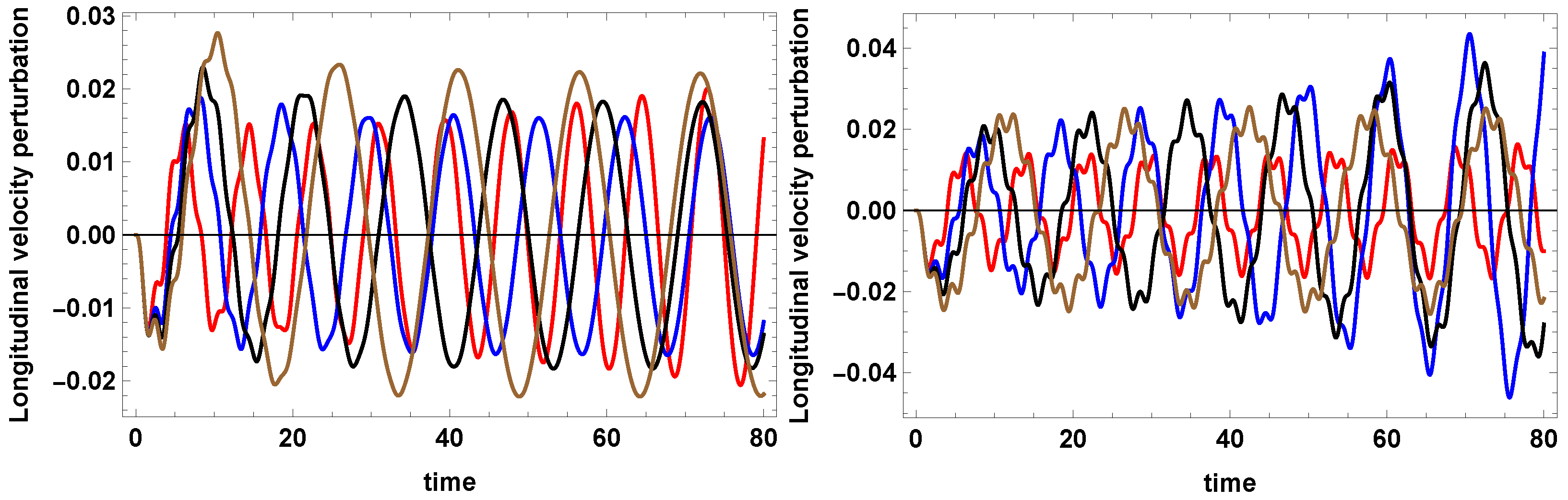
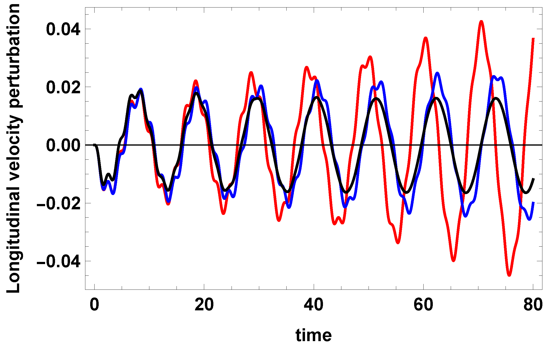
In this Subsection, the density dependence of the heating mechanism remains the same, because temperature dependence is modified by increasing exponent b from 4 up to . Figure 4 (left), corresponding to m, shows that, for the considered a and b parameters, the longitudinal velocity perturbations are amplified by the amplifying thermal times as follows: T = 12,000 K, s; K, s; K, 15,840 s; and K, 215,000 s. As noted above, the minus sign is due to the negative sign of the quantity in Equation (31): thus, , and one has amplification of thermal origin. An interesting conclusion, which is derived from Section 3.1, Section 3.2 and Section 3.3, is that by keeping a constant and increasing the exponent b of the temperature, the behavior of the perturbations changes from damping for to a weaker damping for , and to an amplification for ; therefore, it seems that if, in the heating mechanism, the density dependence is kept constant and the temperature dependence is made stronger, then the temporal behavior of the perturbations goes from damping to amplification. The effect of the ambipolar diffusion is the same here as in Figure 3 (left), because the ambipolar diffusion damping times are not influenced by the heating mechanisms. However, it is also important to remark that the effect of ambipolar diffusion is always to damp the perturbations, which is observable at the short times in the brown curve corresponding to the lowest temperature and highest Cowling’s diffusivity. In spite of this damping effect, the thermal effects are still able to amplify the perturbations, in such a way that the net result, once both contributions are taken into account, is the temporal amplification of the perturbations. Figure 4 (right), corresponding to m, shows the presence of amplification too. Here, the amplifying thermal times are for T = 12,000 K, 223,580 s; for K, 34,720 s; for K, 22,810 s; and for K, 216,530 s, which are greater than for m, due to the decrease in the wavenumber in Equation (31). This fact implies that for m, the amplification should have proceeded at a weak rate; however, because the effect of ambipolar diffusion is also much weaker, the joint effect gives place to a stronger amplification of the perturbations.
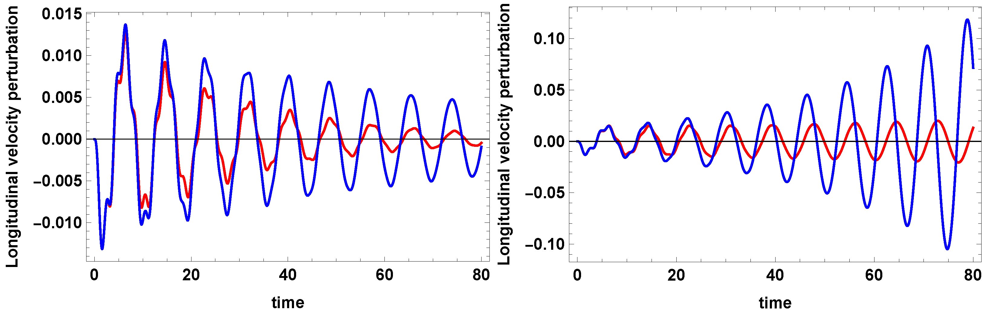
This interplay between thermal effects and ambipolar diffusion can be seen in Figure 5. Figure 5 shows the temporal behavior of longitudinal velocity perturbations for three different values of , modifying the wavenumber and , and a constant temperature K. For m, , = 246,512 s and 34,720 s, the ambipolar diffusion damping time is quite long, while the thermal time is shorter, and the amplification due to thermal effects is dominant (red curve), and appears quickly enough. For m and , s and s; both times are of the same order, and the amplification proceeds slowly (blue curve). For m and , s and s, and the damping due to ambipolar diffusion is strong, in particular at short times (black curve). Finally, as time passes, the effect of ambipolar diffusion decreases, while the amplification due to thermal effects increases; therefore, it takes much longer time to observe the amplification of the oscillations.
The damping effect of ambipolar diffusion is characterized by the behavior of , while amplifying/damping of thermal effects can be understood by assuming that they are characterized by : using these two expressions, one can understand the temporal behavior of the longitudinal velocity perturbations. is always positive; then, when and are both positive, there is a combination of the damping effects; if at the beginning, the damping is dominated by thermal effects and, later, the effect of ambipolar diffusion appears. When , the opposite happens. When , with , there is a competition between the damping effect of ambipolar diffusion and the amplification due to thermal effects: first, one can have amplification, and later, the damping effect appears, or the other way round.
3.4. , , or
In Section 3.2 and Section 3.3, the numerical value of exponent a, which describes the density dependence of the heating mechanism, is kept constant. while the b exponent describing the temperature dependence is modified. One could have proceeded the other way round, keeping constant b and varying a in order to compare to the results obtained in previous Subsections.
Figure 6 compares several heating mechanisms considered at a constant m and temperature T = 12,000 K. The comparison between the temporal behaviors of the longitudinal velocity perturbations for , and , is shown in Figure 6 (left). One can see that for , the damping of the oscillation is stronger than for . The reason is that modifying a and b produces a modification of thermal misbalance times, and , while the ambipolar diffusion damping times, , are not affected. This modification of thermal misbalance times leads to a change of , which is equal to 75 s for , while it is 275 s for and, consequently, the damping for is weaker than for . On the other hand, Figure 6 (right) compares the other two mechanisms, and it shows that, for , amplification proceeds faster than for : again, the reason is a change of , which is equal to s for , while it is equal to for . Summarizing, the results obtained here show that keeping constant the exponent describing the density dependence, while varying the exponent describing the temperature dependence, produces different damping or amplification rates, with respect to the case, in which the exponent describing the temperature dependence is kept constant, while the exponent describing the density dependence is varied. The reason is that thermal misbalance times are modified by these changes, leading to different damping or amplifying thermal times, which weakens or enhances the oscillations, despite the global temporal behavior being similar.
3.5. ,
Section 3.1, Section 3.2, Section 3.3 and Section 3.4 discussed the damping or amplification of the longitudinal velocity perturbations when different heating mechanisms are considered. However, another situation, which may be worth studying, is one, in which the combination of the chosen radiative loss function and heating mechanism gives place to thermal misbalance times, and , having the same numerical value. Then, the approximate analytical expression for the imaginary part of the frequency (Equation (28)) becomes equal to zero and, therefore, the thermal damping or amplifying time becomes infinite, i.e., there is neither damping nor amplification due to thermal effects. However, although in this situation there is no damping or amplification of thermal origin, damping by ambipolar diffusion is always present and, as a consequence, the oscillations should be damped with the characteristic damping time, .
Using Equations (23) and (24), and once a value for a is assumed, one obtains an equation giving the threshold value for b, which separates the regimes of damping and amplification due to thermal effects:
On the other hand, once exponent b is fixed, using Equation (32), one also obtains an expression for the threshold value of exponent a, which is
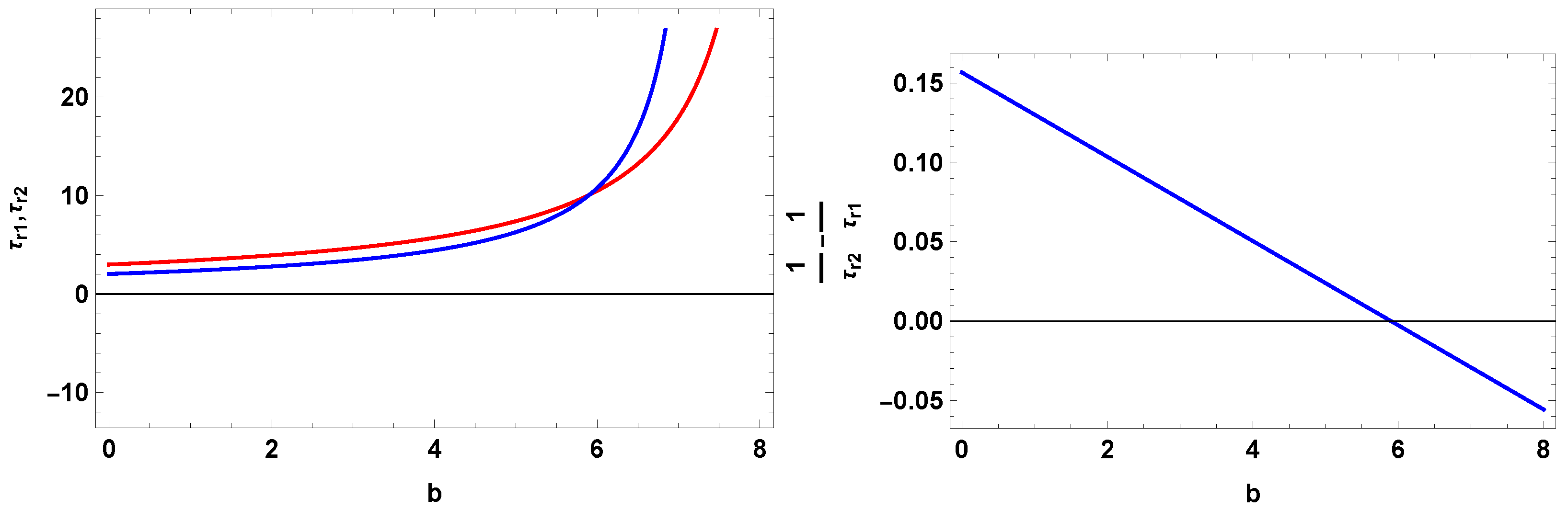
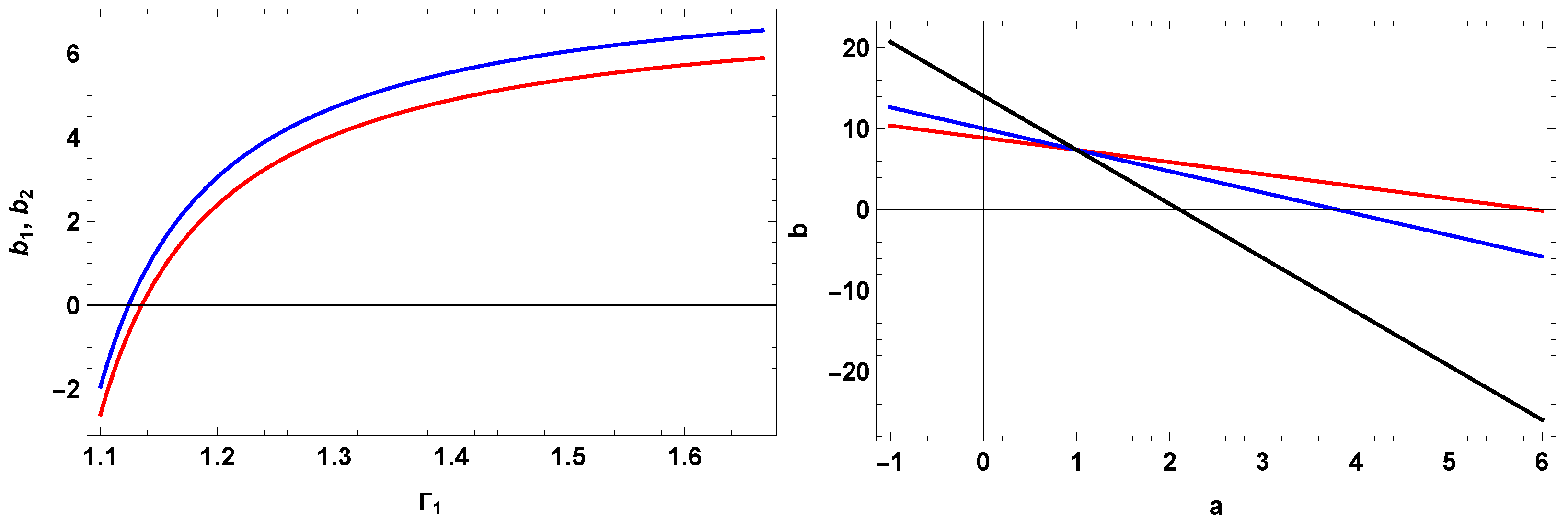
Assuming a radiative loss function, along with numerical values for a and , one obtains a numerical value for b that satisfies Equation (32): for instance, taking , and [42] from Equation (32), one obtains . Another possibility is that, with assumed numerical values for b and , the value of a can be determined, satisfying Equation (33). Figure 7 (left) displays the behavior of thermal misbalance times versus the b exponent. In the beginning, is smaller than , but for a certain value of b, both curves crossed and becomes larger than . Figure 7 (right) shows the behavior of the expression − versus the b exponent, and one can see that this difference becomes zero for , as one can find from Equation (32).
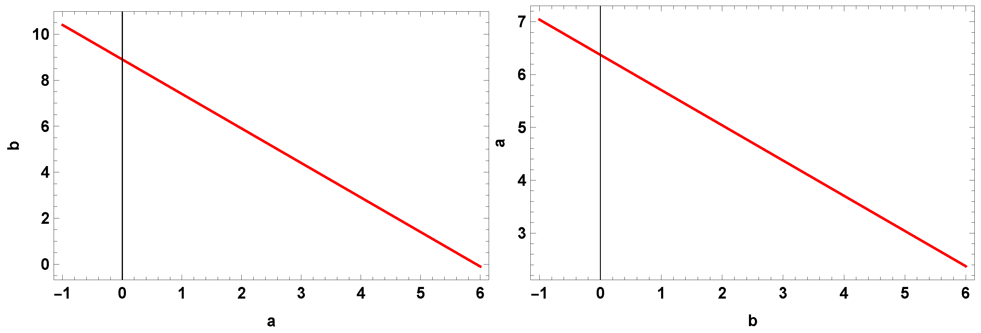
On the other hand, Figure 8 (left), for , shows the behavior of the threshold values of the b exponent, when exponent a varies between and 6, while Figure 8 (right), displays the behavior of the a exponent when the b exponent varies between and 6. In both cases, the behavior is linear, as can be expected from Equations (32) and (33), but if the same value for a fixed in Figure 8 (left) is used for b in Figure 8 (right), the corresponding values for b and a are different, which explains the results obtained in Section 3.4. Summarizing, in Figure 8 (left panel), fixing a value of a, for those values of b below the straight line, one finds damping of the oscillations, while for those above the line, one finds amplification of the oscillations. The same behavior for a can be found in Figure 8 (right) when b is fixed.
In order to highlight the case when , let us consider T = 12,000 K. Figure 9 (left) shows the behavior of − versus an interval of numerical values for exponents a and b. One can observe how this difference evolves from positive to negative values, going through zero, when a and b are varied within the considered interval: Figure 9 (right) shows the evolution of the imaginary part of the frequency , computed by Equation (28), within the interval of numerical values considered for a and b. From Figure 9 (right) one can see that the imaginary frequency also goes from positive to negative values, becoming zero for certain pairs of a and b values. Next, Figure 10 (left) shows the variation of the thermal time, , and demonstrates a discontinuity, which well highlights that, for certain pairs of values of a and b, the thermal time becomes infinite, corresponding to . Figure 10 (right) shows, for a reduced interval of values of a and b, a comparison between the thermal time and the ambipolar diffusion time, which is constant once the temperature is fixed.
Finally, imposing and , Figure 11 (left) displays the temporal behavior of the oscillations for K. The damping by ambipolar diffusion proceeds as which, in this case, and since s, would be , and Figure 11 (left) shows that the damping due to ambipolar diffusion produced a decay of the oscillations, well seen at short times; later, when time increases, the damping proceeds more slowly and, because damping due to thermal effects is absent, the general impression is that the oscillations are almost decayless. In case the ambipolar diffusion time, , is quite long, the damping due to this effect takes a long time to be visible in the oscillatory plots, enhancing the impression of decayless oscillations. Complete decayless oscillations would only be possible for an infinite ambipolar diffusion time that can be obtained only by imposing (no wave) or , which cannot be attained, because for fully ionized plasma, Spitzer’s diffusivity is equal to Cowling’s diffusivity, .
3.6. LTE and NLTE
Until this point, the calculations assumed that the adiabatic coefficient, , is constant and equal ; however, it is known that, in the case of partially ionized plasmas, this assumption is not satisfied. For a partially ionized hydrogen gas, the dependence of on temperature and ionization degree has been computed [54,55,56,57]. Here, instead of considering the adiabatic coefficient , the first adiabatic exponent,
is introduced, where the derivative is computed at constant entropy, s. This coefficient is equal to for a fully neutral or ionized gas, although its numerical value depends on the ionization degree, temperature and density. Considering the ionization degrees obtained from the NLTE model, can be computed, while, for comparison, also LTE is assumed, and the corresponding ionization degree and are computed using a modified Saha equation (for details of the computations see [33]). Figure 11 (right) shows the behavior of both the LTE and the NLTE versus the temperature. As one can see, for the considered temperature interval, there is a sensitive difference between the two-model exponents, which is basically due to the consideration of the LTE and NLTE models, on which the calculation of is based. However, for temperatures around 14,000 K, corresponding to full ionization, both exponents converged to the same value of , as expected.
On the other hand, if in the equations where is involved, instead of , is considered, then the equations to be modified by the variation, with temperature and ionization degree, of LTE and NLTE are: the specific heat, , in which decreasing would mean increasing ; while thermal misbalance times, and , would depend on and , and the decrease of would increase both times. Furthermore, sound speed would decrease with and, as a consequence, the frequency given by would also decrease while the associated period is increased. Finally, the approximate analytical solution in Equation (28) is also modified, because terms, such as , and , are involved. However, other expressions, such as ones for and , remain unchanged.
3.7. , LTE and NLTE , or
Here, and as an example, for K, the temporal behaviors of the longitudinal velocity perturbations for a constant , NLTE and LTE , are compared. Again, two heating mechanisms characterized by and , are considered. The results are shown in Figure 12. Figure 12 (left) displays the results for , and one can see that, while for , oscillation are damped with a damping time s, for LTE , s, which means a weak damping of the oscillation, while for NLTE one finds a thermal amplifying time of s, and the oscillations are amplified. This behavior can be understood following Equation (32), because taking , and , the threshold value for b, to change the behavior from damping to amplification, is , same as found in Section 3.5. However, taking LTE , the threshold value was , and for NLTE , the threshold value of b is , which explains the presence of amplification in this case. Furthermore, in the case of NLTE , the period is increased, because the sound speed decreases with respect to the other cases, leading to a decrease of . Figure 12 (right) corresponds to and, in this case, all the oscillations are amplified by the amplifying times given by for constant , for LTE and s for NLTE ; therefore, one finds amplification, because all the cases satisfy the threshold values mentioned. Different amplifying times are obtained that means that the rates, at which the oscillations are amplified, are different. These results point out that the consideration of the first adiabatic exponent, and how it varies by temperature and ionization degree since the density is kept constant, is important in order to properly describe the temporal behavior of the longitudinal velocity perturbations associated with the slow waves, and that these variations could even cause a complete change of behavior with respect to a constant that has been considered in many studies. It is also important to remark that, once the temperature and are fixed in the present calculations, the ambipolar diffusion damping time is fixed as well.
4. CHIANTI7 Radiative Loss Function
This Section considers the CHIANTI7 optically thin radiative function [43,44,45] and a constant , and the results are shown in Figure 13. Figure 13 (left) shows that, for , , the general behavior of the oscillations is the same as for the Hildner radiative loss function, and the only differences are visible for the thermal damping times, such as 220 s, 104 s, 609 s, and 10,780 s. For , those times are 396 s, 702 s, 5007 s and 89,024 s, which means that there is no amplification of the oscillations, and is a completely different behavior than that in the case of the Hildner [42] optically thin radiative function. The reason for this behavior is that, in Equation (32), the value of is now instead of , and amplification appears for the values of b above . However, in order to illustrate the effect that could have on the oscillatory behaviors, setting K, NLTE , LTE , , and , the above results change. For the NLTE , the threshold value for b is , and for the LTE , it is , both values being smaller than ; the latter means that, in both cases, the oscillations are going to be amplified. Therefore, by modifying the numerical value of the first adiabatic exponent, one is able to modify the temporal behavior of oscillations.
Next, using Equation (32), for , Figure 14 (left) shows the behavior of the threshold values of the b exponent versus for the two values of corresponding to the Hildner [42] and CHIANTI7 radiative functions [43,44,45]. One can observe that, for a fixed value of , the difference between the two curves is small; however, there is quite a difference between the values of b for small and large values of . Figure 14 (right) displays the behavior of the threshold values of exponent b versus exponent a for the three different values of and, for a fixed value of a, the effect of the numerical value of the first adiabatic exponent on b is visible. Furthermore, and similar to that observed in Section 3.5, once a value of a is fixed, for those values of b below the straight lines, there is a damping of the oscillations, while for the b values above the lines one finds and amplification of the oscillations. On the other hand, due to the crossing of the straight lines one can conclude that both the amplification and damping are dependent on the value of .
Recapitulating, the two radiative functions considered produce a change in the damping or amplifying rates of the oscillations, because the functions modify the misbalance thermal times, which modify the thermal time, ; however, the consideration of the first adiabatic exponent and its variation with temperature and ionization degree could also produce important changes in the oscillatory behavior.
5. Discussion
Observations have shown the presence of damped/amplified oscillations in prominences which are made of partially ionized plasmas, and these oscillations have been mostly interpreted in terms of MHD waves. Different damping mechanisms of thermal origin, like radiation and thermal conduction, have been proposed, although in most of the cases fully ionized plasmas have been considered. When partially ionized plasmas are considered, ambipolar diffusion introduces a further dissipative mechanism, contributing to the damping. However, to understand the amplification process of the oscillations another mechanism is needed.
Taking advantage of the nonlinear coupling of Alfvén and slow magnetoacoustic waves, the present study investigated the temporal behavior of the field-aligned motions, representing slow waves, generated by the ponderomotive force in an unbounded partially ionized prominence plasma. In the calculations made here the heating–cooling misbalance, with heating mechanisms depending on powers of density and temperature as well as ambipolar diffusion, were considered. First of all, the joint effect of thermal misbalance with different heating mechanisms characterized by different dependences on density and temperature and ambipolar diffusion allowed us to obtain different oscillatory behaviors showing damping or amplification. As ambipolar diffusion is a dissipative mechanism, the characteristic time, , was always found to be positive; therefore, the amplification of the oscillations is of thermal origin. The comparison between the thermal time, , characterizing the damping or amplification of thermal origin, and the ambipolar diffusion time, , were shown to determine the temporal behavior of the oscillations. When the thermal time was taken positive, the oscillations were observed to be damped, due to the joint effect of thermal mechanisms and ambipolar diffusion characterized by and , respectively. However, for the negative thermal time, the effect was an amplification of the oscillations, combined with a damping produced by ambipolar diffusion. In this case, if , initially, the effect of the damping produced by ambipolar diffusion was strong and, later on, the amplifying effect started to be present; conversely, when , the opposite behavior occurred. An interesting case was observed when thermal misbalance of the times, and , were equal, which means that there is no damping or amplification of thermal origin: this condition allowed us to determine threshold values for the exponents a and b, describing the density and temperature dependences of the heating mechanisms. These threshold values were found to locate along the straight lines defining the borders between two regions: in one region, the oscillations were damped, while in the other region the oscillations were amplified. In both cases, superimposed by these behaviors, there was a damping effect observed, due to ambipolar diffusion.
On the other hand, although a partially ionized plasma was considered, in the reported study, a constant value for the adiabatic coefficient was assumed. Therefore, in order to be coherent with the kind of plasma under study, and to determine how the results obtained can be affected by this consideration, three different cases were compared, namely: a constant , and the first adiabatic exponent, , computed under NLTE and LTE conditions, whose numerical value depended on density, temperature and ionization degree. The results showed that quite strong differences appear in the temporal behavior of the oscillations and, basically, these differences were the changes in the rates of damping or amplification, as well as being modifications of the behavior from damping to amplification or the other way round. Certainly, taking into account the different numerical values for constant , LTE and NLTE , the border between the regions separating damping from amplification of thermal origin was modified, straightforwardly pointing out, the influence of these parameters on the results. Furthermore, the consideration of Hildner [42] or CHIANTI7 radiative loss functions [43,44,45] were also found to modify the separation between damping and amplification regions in the plane () of the exponents.
Finally, taking into account the above discussed mechanisms and parameters, as well as the obtained results regarding damping or amplification, by varying the parameters describing the prominence plasma physical state, one should be able to match the temporal behavior of the observed prominence oscillations, performing what is called prominence seismology. In this sense, and in a simpler case of only thermal effects, the matching between theory and observations of damped and amplified small amplitude oscillations in prominences, has been achieved [32]. However, in the case studied here, and because of the joint consideration of thermal effects and ambipolar diffusion, a similar study would imply that, in order to perform the matching, one would need to consider an additional parameter, such as .
Funding
This publication is part of the R+D+i (Research, Development, and innovation) project PID2020-112791GB-I00, financed by MCIN/AEI/10.13039/501100011033 (Spain).
Data Availability Statement
Not applicable.
Acknowledgments
The author would like to acknowledge Marcel Goossens for his leadership in MHD waves, which has always been a source of inspiration. This research was supported by the International Space Science Institute (ISSI) in Bern, Switzerland, through the ISSI International Team project 457 (The Role of Partial Ionization in the Formation, Dynamics and Stability of Solar Prominences).
Conflicts of Interest
The author declares no conflict of interest.
Appendix A
References
- Tomczyk, S.; McIntosh, S.W.; Keil, S.L.; Judge, P.G.; Schad, T.; Seeley, D.H.; Edmondson, J. Alfvén waves in the solar corona. Science 2007, 317, 1192–1196. [Google Scholar] [CrossRef] [PubMed]
- Jess, D.B.; Mathioudakis, M.; Erdélyi, R.; Crockett, P.J.; Keenan, F.P.; Christian, D.J. Alfvén waves in the lower solar atmosphere. Science 2009, 323, 1582–1585. [Google Scholar] [CrossRef] [PubMed] [Green Version]
- Mathioudakis, M.; Jess, D.B.; Erdélyi, R. Alfvén waves in the solar atmosphere. From theory to observations. Space Sci. Rev. 2013, 175, 1–27. [Google Scholar] [CrossRef] [Green Version]
- Srivastava, A.K.; Shetye, J.; Murawski, K.; Doyle, J.G.; Stangalini, M.; Scullion, E.; Ray, T.; Wójcik, D.P.; Dwivedi, B.N. High-frequency torsional Alfvén waves as an energy source for coronal heating. Sci. Rep. 2017, 7, 43147. [Google Scholar] [CrossRef]
- Grant, S.D.T.; Jess, D.B.; Zaqarashvili, T.V.; Beck, C.; Socas-Navarro, H.; Aschwanden, M.J.; Keys, P.H.; Christian, D.J.; Houston, S.J.; Hewitt, R.L. Alfvén wave dissipation in the solar chromosphere. Nat. Phys. 2018, 14, 480–483. [Google Scholar] [CrossRef] [Green Version]
- Kohutova, P.; Verwichte, E.; Froment, C. First direct observation of a torsional Alfvén oscillation at coronal heights. Astron. Astrophys. 2020, 633, L6. [Google Scholar] [CrossRef] [Green Version]
- Cramer, N.F. The Physics of Alfvén Waves; WILEY-VCH Verlag Berlin GmbH: Berlin, Germany, 2001. [Google Scholar] [CrossRef]
- Hollweg, J.V. Density fluctuations driven by Alfvén waves. J. Geophys. Res. 1971, 76, 5155–5161. [Google Scholar] [CrossRef]
- Rankin, R.; Frycz, P.; Tikhonchuk, V.T.; Samson, J.C. Nonlinear standing shear Alfvén waves in the Earth’s magnetosphere. J. Geophys. Res. 1994, 99, 21291–21302. [Google Scholar] [CrossRef]
- Tikhonchuk, V.T.; Rankin, R.; Frycz, P.; Samson, J.C. Nonlinear dynamics of standing shear Alfvén waves. Phys. Plasmas 1995, 2, 501–515. [Google Scholar] [CrossRef]
- Terradas, J.; Ofman, L. Loop density enhancement by nonlinear magnetohydrodynamic waves. Astrophys. J. 2004, 610, 523–531. [Google Scholar] [CrossRef]
- Zaqarashvili, T.V.; Carbonell, M.; Ballester, J.L.; Khodachenko, M.L. Cut-off wavenumber of Alfvén waves in partially ionized plasmas of the solar atmosphere. Astron. Astrophys. 2012, 544, A143. [Google Scholar] [CrossRef]
- Soler, R.; Carbonell, M.; Ballester, J.L. On the Spatial scales of wave heating in the solar chromosphere. Astrophys. J. 2015, 810, 146. [Google Scholar] [CrossRef] [Green Version]
- Soler, R.; Ballester, J.L.; Zaqarashvili, T.V. Overdamped Alfvén waves due to ion-neutral collisions in the solar chromosphere. Astron. Astrophys. 2015, 573, A79. [Google Scholar] [CrossRef]
- Soler, R.; Terradas, J.; Oliver, R.; Ballester, J.L. The role of Alfvén wave heating in solar prominences. Astron. Astrophys. 2016, 592, A28. [Google Scholar] [CrossRef] [Green Version]
- Cally, P.S.; Khomenko, E. Fast-to-Alfvén mode conversion in the presence of ambipolar diffusion. Astrophys. J. 2018, 856, 20. [Google Scholar] [CrossRef]
- González-Morales, P.A.; Khomenko, E.; Cally, P.S. Fast-to-Alfvén mode conversion mediated by hall current. II. Application to the solar atmosphere. Astrophys. J. 2019, 870, 94. [Google Scholar] [CrossRef] [Green Version]
- Khomenko, E.; Cally, P.S. Fast-to-Alfvén mode conversion and ambipolar heating in structured media. II. Numerical simulation. Astrophys. J. 2019, 883, 179. [Google Scholar] [CrossRef]
- Cally, P.S.; Khomenko, E. Fast-to-Alfvén mode conversion and ambipolar heating in Structured media. I. Simplified old plasma model. Astrophys. J. 2019, 885, 58. [Google Scholar] [CrossRef]
- Ballester, J.L.; Soler, R.; Terradas, J.; Carbonell, M. Nonlinear coupling of Alfvén and slow magnetoacoustic waves in partially ionized solar plasmas. Astron. Astrophys. 2020, 641, A48. [Google Scholar] [CrossRef]
- Zavershinskii, D.I.; Kolotkov, D.Y.; Nakariakov, V.M.; Molevich, N.E.; Ryashchikov, D.S. Formation of quasi-periodic slow magnetoacoustic wave trains by the heating/cooling misbalance. Phys. Plasmas 2019, 26, 082113. [Google Scholar] [CrossRef] [Green Version]
- Kolotkov, D.Y.; Nakariakov, V.M.; Zavershinskii, D.I. Damping of slow magnetoacoustic oscillations by the misbalance between heating and cooling processes in the solar corona. Astron. Astrophys. 2019, 628, A133. [Google Scholar] [CrossRef] [Green Version]
- Kolotkov, D.Y.; Duckenfield, T.J.; Nakariakov, V.M. Seismological constraints on the solar coronal heating function. Astron. Astrophys. 2020, 644, A33. [Google Scholar] [CrossRef]
- Belov, S.; Molevich, N.; Zavershinskii, D. Thermal misbalance influence on the nonlinear shear Alfvén waves under solar atmosphere conditions. Sol. Phys. 2020, 295, 160. [Google Scholar] [CrossRef]
- Prasad, A.; Srivastava, A.K.; Wang, T.J. Role of compressive viscosity and thermal conductivity on the damping of slow waves in coronal loops with and without heating-cooling imbalance. Sol. Phys. 2021, 296, 20. [Google Scholar] [CrossRef]
- Prasad, A.; Srivastava, A.K.; Wang, T. Effect of thermal conductivity, compressive viscosity and radiative cooling on the phase shift of propagating slow waves with and without heating-cooling imbalance. Sol. Phys. 2021, 296, 105. [Google Scholar] [CrossRef]
- Belov, S.; Vasheghani Farahani, S.; Molevich, N.; Zavershinskii, D. Longitudinal plasma motions generated by shear Alfvén waves in plasma with thermal misbalance. Sol. Phys. 2021, 296, 98. [Google Scholar] [CrossRef]
- Zavershinskii, D.; Kolotkov, D.; Riashchikov, D.; Molevich, N. Mixed properties of slow magnetoacoustic and entropy waves in a plasma with heating/cooling misbalance. Sol. Phys. 2021, 296, 96. [Google Scholar] [CrossRef]
- Belov, S.A.; Molevich, N.E.; Zavershinskii, D.I. Dispersion of slow magnetoacoustic waves in the active region fan loops introduced by thermal misbalance. Sol. Phys. 2021, 296, 122. [Google Scholar] [CrossRef]
- Prasad, A.; Srivastava, A.K.; Wang, T.; Sangal, K. Role of non-ideal dissipation with heating-cooling misbalance on the phase shifts of standing slow magnetohydrodynamic waves. Sol. Phys. 2022, 297, 5. [Google Scholar] [CrossRef]
- Kolotkov, D.Y.; Zavershinskii, D.I.; Nakariakov, V.M. The solar corona as an active medium for magnetoacoustic waves. Plasma Phys. Control. Fusion 2021, 63, 124008. [Google Scholar] [CrossRef]
- Ibañez, M.H.; Ballester, J.L. The effect of thermal misbalance on slow magnetoacoustic waves in a partially ionized prominence-like plasma. Sol. Phys. 2022, 297, 144. [Google Scholar] [CrossRef]
- Ballester, J.L.; Soler, R.; Carbonell, M.; Terradas, J. The first adiabatic exponent in a partially ionized prominence plasma: Effect on the period of slow waves. Astron. Astrophys. 2021, 656, A159. [Google Scholar] [CrossRef]
- Anzer, U.; Heinzel, P. The energy balance in solar prominences. Astron. Astrophys. 1999, 349, 974–984. Available online: https://adsabs.harvard.edu/full/1999A%26A...349..974A (accessed on 3 March 2023).
- Heinzel, P.; Anzer, U.; Gunár, S. Solar quiescent prominences. Filamentary structure and energetics. Mem. Soc. Astron. Ital. 2010, 81, 654–661. Available online: https://ui.adsabs.harvard.edu/abs/2010MmSAI..81..654H (accessed on 3 March 2023).
- Heinzel, P.; Anzer, U. Radiative equilibrium in solar prominences reconsidered. Astron. Astrophys. 2012, 539, A49. [Google Scholar] [CrossRef] [Green Version]
- Labrosse, N.; Heinzel, P.; Vial, J.C.; Kucera, T.; Parenti, S.; Gunár, S.; Schmieder, B.; Kilper, G. Physics of solar prominences: I—Spectral diagnostics and non-LTE modelling. Space Sci. Rev. 2010, 151, 243–332. [Google Scholar] [CrossRef] [Green Version]
- Heinzel, P. Radiative Transfer in Solar Prominences. In Solar Prominences; Vial, J.-C., Engvold, O., Eds.; Springer International Publishing Switzerland: Cham, Switzerland, 2015; pp. 103–130. [Google Scholar] [CrossRef]
- Parenti, S.; Vial, J.C. Prominence and quiet-Sun plasma parameters derived from FUV spectral emission. Astron. Astrophys. 2007, 469, 1109–1115. [Google Scholar] [CrossRef] [Green Version]
- Parenti, S. Solar prominences: Observations. Living Rev. Sol. Phys. 2014, 11, 1. [Google Scholar] [CrossRef]
- Ballester, J.L.; Alexeev, I.; Collados, M.; Downes, T.; Pfaff, R.F.; Gilbert, H.; Khodachenko, M.; Khomenko, E.; Shaikhislamov, I.F.; Soler, R.; et al. Partially ionized plasmas in astrophysics. Space Sci. Rev. 2018, 214, 58. [Google Scholar] [CrossRef] [Green Version]
- Hildner, E. The Formation of solar quiescent prominences by condensation. Sol. Phys. 1974, 35, 123–136. [Google Scholar] [CrossRef]
- Dere, K.P.; Landi, E.; Mason, H.E.; Monsignori Fossi, B.C.; Young, P.R. CHIANTI—An atomic database for emission lines. Astron. Astrophys. Suppl. 1997, 125, 149–173. [Google Scholar] [CrossRef] [Green Version]
- Landi, E.; Del Zanna, G.; Young, P.R.; Dere, K.P.; Mason, H.E. CHIANTI—An atomic database for emission lines. XII. Version 7 of the database. Astrophys. J. 2012, 744, 99. [Google Scholar] [CrossRef] [Green Version]
- Soler, R.; Ballester, J.L.; Parenti, S. Stability of thermal modes in cool prominence plasmas. Astron. Astrophys. 2012, 540, A7. [Google Scholar] [CrossRef] [Green Version]
- Heinzel, P.; Vial, J.C.; Anzer, U. On the formation of Mg II h and k lines in solar prominences. Astron. Astrophys. 2014, 564, A132. [Google Scholar] [CrossRef]
- Nakariakov, V.M.; Kolotkov, D.Y. Magnetohydrodynamic waves in the solar corona. Annu. Rev. Astron. Astrophys. 2020, 58, 441–481. [Google Scholar] [CrossRef]
- Duckenfield, T.J.; Kolotkov, D.Y.; Nakariakov, V.M. The effect of the magnetic field on the damping of slow waves in the solar corona. Astron. Astrophys. 2021, 646, A155. [Google Scholar] [CrossRef]
- Soler Juan, R. Damping of Magnetohydrodynamic Waves in Solar Prominence Fine Structures. Ph.D. Thesis, Departament de Fisica, Universitat de les Illes Balears, Palma de Mallorca, Spain, 2010. Available online: http://dfs.uib.es/Solar/thesis_robertosoler.pdf (accessed on 3 March 2023).
- Rosner, R.; Tucker, W.H.; Vaiana, G.S. Dynamics of the quiescent solar corona. Astrophys. J. 1978, 220, 643–645. [Google Scholar] [CrossRef]
- Dahlburg, R.B.; Mariska, J.T. Influence of heating rate on the condensational instability. Sol. Phys. 1988, 117, 51–56. [Google Scholar] [CrossRef]
- Ibañez, S.; Miguel, H.; Sanchez, D.; Nestor, M. Propagation of sound and thermal waves in a plasma with solar abundances. Astrophys. J. 1992, 396, 717. [Google Scholar] [CrossRef]
- Ibañez, S.; Miguel, H.; Escalona, T.; Orlando, B. Propagation of hydrodynamic waves in optically thin plasmas. Astrophys. J. 1993, 415, 335. [Google Scholar] [CrossRef]
- Clayton, D.D. Principles of Stellar Evolution and Nucleosynthesis; The University of Chicago Press: Chicago, IL, USA, 1984. [Google Scholar]
- Prialnik, D. An Introduction to the Theory of Stellar Structure and Evolution; Cambridge University Press: Cambridge, UK, 2000. [Google Scholar]
- Hansen, C.J.; Kawaler, S.D.; Trimble, V. Stellar Interiors: Physical Principles, Structure, and Evolution; Springer Science+Business Media: New York, NY, USA, 2004. [Google Scholar] [CrossRef]
- Priest, E. Magnetohydrodynamics of the Sun; Cambridge University Press: New York, NY, USA, 2014. [Google Scholar] [CrossRef] [Green Version]
Figure 1.
Dimensionless longitudinal velocity perturbations versus dimensionless time computed (left) at for T = 12,000 K (red curve), K (blue curve), K (black curve) and K (brown curve); , , ; and (right) at for T = 12,000 K, (red curve), K, (blue curve), K, (black curve) and K, (brown curve). , , . The characteristic length, m, and the Hildner [42] radiative function are used. See text for details.

Figure 2.
Left: Comparison between the numerical solution for the longitudinal velocity perturbation (red curve) and the analytical solution (blue curve) ( K, , ). Right: Temporal behavior of the longitudinal velocity perturbations for different heating mechanisms, with (red curve), (blue curve), (black curve), and (brown curve); K, . m and the Hildner [42] radiative function are used as needed. See text for details.

Figure 3.
Dimensionless longitudinal velocity perturbations versus dimensionless time computed (left) at for T = 12,000 K, (red curve), K, (blue curve), K, (black curve) and K, (brown curve), with m; and (right) at for T = 12,000 K, (red curve), K, (blue curve), K, (black curve) and K, (brown curve); , , , with m. The Hildner [42] radiative function is used. See text for details.

Figure 4.
Dimensionless longitudinal velocity perturbations versus dimensionless time computed (left) at for T = 12,000 K, (red curve), K, (blue curve), K, (black curve) and K, (brown curve), with m; and (right) at for T = 12,000 K, (red curve), K, (blue curve), K, (black curve) and K, (brown curve) with , , , and m. The Hildner [42] radiative function is used. See text for details.

Figure 5.
Dimensionless longitudinal velocity perturbations versus dimensionless time computed at for m (red curve), , m (blue curve), , m (black curve), . K; , . The Hildner [42] radiative function is used.
Figure 5.
Dimensionless longitudinal velocity perturbations versus dimensionless time computed at for m (red curve), , m (blue curve), , m (black curve), . K; , . The Hildner [42] radiative function is used.

Figure 6.
Dimensionless longitudinal velocity perturbations versus dimensionless time computed (left) at for T = 12,000 K, , (red curve) and (blue curve), and (right) at for T = 12,000 K, , (red curve) and (blue curve); . m, and the Hildner [42] radiative function are used.
Figure 6.
Dimensionless longitudinal velocity perturbations versus dimensionless time computed (left) at for T = 12,000 K, , (red curve) and (blue curve), and (right) at for T = 12,000 K, , (red curve) and (blue curve); . m, and the Hildner [42] radiative function are used.

Figure 7.
Left: thermal misbalance times versus b exponent: (red curve), (blue curve). Right: − versus b exponent, T = 12,000 K, , . m and the Hildner [42] radiative function are used. See text for details.
Figure 7.
Left: thermal misbalance times versus b exponent: (red curve), (blue curve). Right: − versus b exponent, T = 12,000 K, , . m and the Hildner [42] radiative function are used. See text for details.

Figure 8.
The threshold values for (left) the b exponent versus the a exponent and for (right) the a exponent versus the b exponent. and the Hildner [42] radiative function are used. See text for details.
Figure 8.
The threshold values for (left) the b exponent versus the a exponent and for (right) the a exponent versus the b exponent. and the Hildner [42] radiative function are used. See text for details.

Figure 9.
(Left): − versus a and b exponents. (Right): versus a and b exponents. T = 12,000 K. The Hildner [42] radiative function is used. See text for details.
Figure 9.
(Left): − versus a and b exponents. (Right): versus a and b exponents. T = 12,000 K. The Hildner [42] radiative function is used. See text for details.

Figure 10.
Thermal time, (left), and (right) (red) and ambipolar diffusion time, (blue), versus a and b exponents. T = 12,000 K. The Hildner [42] radiative function is used. See text for details.
Figure 10.
Thermal time, (left), and (right) (red) and ambipolar diffusion time, (blue), versus a and b exponents. T = 12,000 K. The Hildner [42] radiative function is used. See text for details.

Figure 11.
Left: dimensionless longitudinal velocity perturbations versus dimensionless time, computed at for m, K, , , and . The Hildner [42] radiative function is used. Right: LTE first adiabatic exponent, (blue curve) and NLTE (red curve) versus temperature. See text for details.
Figure 11.
Left: dimensionless longitudinal velocity perturbations versus dimensionless time, computed at for m, K, , , and . The Hildner [42] radiative function is used. Right: LTE first adiabatic exponent, (blue curve) and NLTE (red curve) versus temperature. See text for details.

Figure 12.
Dimensionless longitudinal velocity perturbations versus dimensionless time computed (left) at for K, , (red curve), , LTE (blue curve), , NLTE (black curve), , , and (right) at for K, , (red curve), , LTE (blue curve), , NLTE (black curve), , . . m and the Hildner [42] radiative function are used.

Figure 13.
Dimensionless longitudinal velocity perturbations versus dimensionless time computed (left) at for T = 12,000 K, (red curve), K, (blue curve), K, (black curve) and K, (brown curve), with and , and (right) at for T = 12,000 K, (red curve), K, (blue curve), K, (black curve) and K, (brown cirve), with and . The CHIANTI7 radiative function [43,44,45] is used.

Figure 14.
The threshold values of (left) the b exponent versus for Hildner [42] (red curve) and CHIANT7 (blue curve) radiative loss functions with , and (right) of the b exponent versus the exponent a for (red curve), (blue curve), (black curve) using the CHIANTI7 radiative loss function.
Figure 14.
The threshold values of (left) the b exponent versus for Hildner [42] (red curve) and CHIANT7 (blue curve) radiative loss functions with , and (right) of the b exponent versus the exponent a for (red curve), (blue curve), (black curve) using the CHIANTI7 radiative loss function.

Disclaimer/Publisher’s Note: The statements, opinions and data contained in all publications are solely those of the individual author(s) and contributor(s) and not of MDPI and/or the editor(s). MDPI and/or the editor(s) disclaim responsibility for any injury to people or property resulting from any ideas, methods, instructions or products referred to in the content. |
© 2023 by the author. Licensee MDPI, Basel, Switzerland. This article is an open access article distributed under the terms and conditions of the Creative Commons Attribution (CC BY) license (https://creativecommons.org/licenses/by/4.0/).
Share and Cite
MDPI and ACS Style
Ballester, J.L. Nonlinear Coupling of Alfvén and Slow Magnetoacoustic Waves in Partially Ionized Solar Plasmas: The Effect of Thermal Misbalance. Physics 2023, 5, 331-351. https://doi.org/10.3390/physics5020025
AMA Style
Ballester JL. Nonlinear Coupling of Alfvén and Slow Magnetoacoustic Waves in Partially Ionized Solar Plasmas: The Effect of Thermal Misbalance. Physics. 2023; 5(2):331-351. https://doi.org/10.3390/physics5020025
Chicago/Turabian StyleBallester, José Luis. 2023. "Nonlinear Coupling of Alfvén and Slow Magnetoacoustic Waves in Partially Ionized Solar Plasmas: The Effect of Thermal Misbalance" Physics 5, no. 2: 331-351. https://doi.org/10.3390/physics5020025