Article

Thermosolutal Marangoni Convection for Hybrid Nanofluid Models: An Analytical Approach

by
Ulavathi Shettar Mahabaleshwar
1,
Rudraiah Mahesh
1 and
Filippos Sofos
2,*
1
Department of Studies in Mathematics, Davangere University, Shivagangothri, Davangere 577 007, India
2
Condensed Matter Physics Laboratory, Department of Physics, University of Thessaly, 35100 Lamia, Greece
*
Author to whom correspondence should be addressed.
Physics 2023, 5(1), 24-44; https://doi.org/10.3390/physics5010003
Submission received: 24 September 2022 / Revised: 10 December 2022 / Accepted: 16 December 2022 / Published: 29 December 2022
(This article belongs to the Section Statistical Physics and Nonlinear Phenomena)

Abstract

:
The present study investigates the effect of mass transpiration on heat absorption/generation, thermal radiation and chemical reaction in the magnetohydrodynamics (MHD) Darcy–Forchheimer flow of a Newtonian fluid at the thermosolutal Marangoni boundary over a porous medium. The fluid region consists of H2O as the base fluid and fractions of TiO2–Ag nanoparticles. The mathematical approach given here employs the similarity transformation, in order to transform the leading partial differential equation (PDE) into a set of nonlinear ordinary differential equations (ODEs). The derived equations are solved analytically by using Cardon’s method and the confluent hypergeometric function. The solutions are further graphically analyzed, taking into account parameters such as mass transpiration, chemical reaction coefficient, thermal radiation, Schmidt number, Marangoni number, and inverse Darcy number. According to our findings, adding TiO2–Ag nanoparticles into conventional fluids can greatly enhance heat transfer. In addition, the mixture of TiO2–Ag with H2O gives higher heat energy compared to the mixture of only TiO2 with H2O.

1. Introduction

The thermosolutal Marangoni convection (TS-MC) has attracted the interest of the scientific and engineering community during the past decades, as it has been bound to applications in fields such as aviation, crystal growth, semiconductor manufacturing and cooling, thin liquid layer scattering, nuclear reactors, silicon wafers, and bio-medicine [1,2,3]. The MC flow is caused by variation in the surface tension parallel to an interface between two fluids, e.g., a gas and a liquid. In such cases, shear stresses appear, and fluid flow is enhanced.
In an early approach [4,5], it has been shown that the surface tension is affected by temperature in thermocapillary convection. Moreover, by adding small amounts of surfactant materials, surface tension may alter dramatically. In Ref. [6], a numerical investigation based on Keller-box and superposition methods was incorporated for forced TS-MC across a porous surface. Al-Mudhaf et al. [7] investigated the effect of the application of a magnetic field on the TS-MC flow of an electrochemical fluid in porous media, along with heat absorption/generation and chemical process effects. The analytical procedure for TS-MC in the presence of heat transport generation or consumption is investigated in Ref. [8], while the effect of mass transpiration on a Newtonian fluid on TS-MC over a porous boundary connection with chemical radiation and heat generation/absorption has also been a matter of research in Ref. [9]. Other significant contributions in the field include studies on the unsteady magnetohydrodynamics (MHD) in TS-MC flow with mass transformation across an unstable stretched sheet [10] and the optimization of heat and mass transformation in TS-MC of nanomaterials with the cross-diffusion effect [11].
Nowadays, efforts in science and engineering are directed to hybrid nanofluid investigation, due to its advanced heat transfer characteristics and wide applicability in manufacturing and the medical field [12,13,14]. The term “hybrid” refers to two or more distinct nanoparticles with various physio-chemical characteristics, combined to form a homogeneous phase. Towards improving traditional fluid properties, the concept of hybrid nanofluid (HNF) was introduced [15,16]. Conventional fluids, such as water, have poor thermal characteristics and HNFs can improve their performance [17,18]. Tripathi [19] has studied the effect of MHD MC in an unstable thin film with HNF flow over a disc; the effects of TS-MC for a non-Newtonian Casson HNF flow over a rotating disc has been studied in Ref. [20], while in Ref. [21], it has been found that the magnetic parameter improves the heat transfer rate.
Another significant component in TS-MC flows is the surface medium it employs. Fluid momentum in a porous medium is described by Darcy’s law, which connects fluid velocity, pressure gradient, and gravitational force. In this model, flow is presented by Darcy as a macroscopic equation, which is applicable to media with low porosity, low Reynolds numbers, and Newtonian fluid flow. However, when the distribution of the medium pores is varied and their sizes are large, porosity is somehow high, and as a result, the viscous shear increases in accordance with Darcy’s resistance. Using Darcy’s concept as a base, Forchheimer [22] expanded the model in order to calculate the inertial forces by modifying Darcy’s law to include the square of velocity term in the momentum equation. Later, Muskat [23] added this term, which is now known as the “Forchheimer term”, to his study. Hayat et al. [24] investigated the effect of carbon nanotubes (CNTs) on the rotating disk by using the Darcy–Forchheimer model. Ganesh et al. [25] have also analyzed the effect of second order slip and viscous and ohmic dissipations on a porous stretching/shrinking sheet by using the Darcy–Forchheimer model. Towards this direction, Muhammad et al. [26] have also applied the model to investigate the fluid flow in a Maxwell nanofluid with a convective boundary condition, while Jawad et al. [27] have investigated the boundary layer flow on the Marangoni convection. Similar studies include the investigation of the effect of TS-MC of a viscous liquid via a micro cylindrical porous flow in the existence of an axial electric field [28], and laminar MHD on TS-MC along a horizontal surface with the effect of Dufour and Soret [29].
Of particular importance in high-temperature industrial operations is the radiation effect. Using the Rosseland approximation, the heat flux energy distribution is exploited to investigate the outcome of the thermal radiation on convection fluid flow through a stretched sheet [30]. The impact of thermal MC of a magneto-Casson fluid flow over dust particles has been also examined in Ref. [31]. Lin et al. [32] have employed four distinct nanofluids to explore the effect of radiation on MC and heat transfer characteristics in non-Newtonian pseudo-plastic.
Another point worth mentioning is the presence of heat sources/sinks in the flow model, which has a major impact on heat transfer characteristics, as there is a significant temperature difference between the fluid and the surface. During the development of flow models, the special effects of chemical reactions on porous boundary layer flow (BLF) are also taken into account. Patil and Pop [33] have examined the chemical reaction in a vertical cone-induced mixed convection flow. The effect of chemical reactions and heat generation/consumption on MC fluid flow has been studied by Li et al. [34]. There are numerous efforts presented in current literature concerning heat transmission and thermal radiation impact on various geometries [35,36,37,38].
To rationalize our contribution to the field, in the present paper, we employ a hybrid nanofluid (TiO2-AG on H2O base) on the MHD TS-MC with chemically radiative Newtonian fluid flow, in the presence of heat sources/sinks, where the analytical solution is obtained by applying Cardon’s method and confluent hypergeometric functions. A number of parameters affecting the flow is further discussed, such as the impact of volume fraction, inverse Darcy number, Marangoni number, magnetic field, heat source/sink, thermal radiation, Schmidt number, chemical reaction coefficient, and mass transpiration parameter. In the following Sections, the theoretical model is presented, along with the mathematical solutions, and results are discussed.

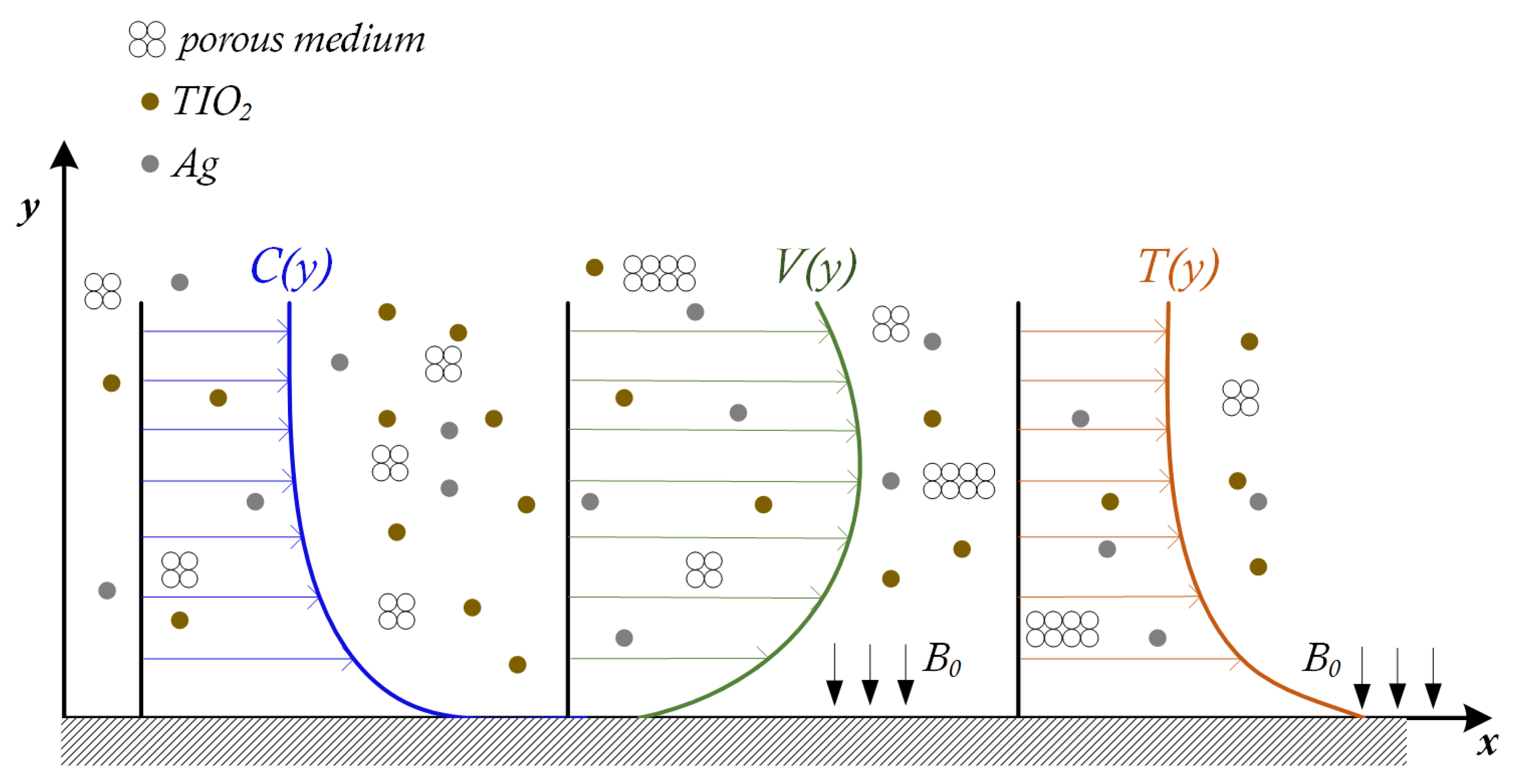
2. Mathematical Model for the Flow Problem

The two-dimensional MHD Newtonian fluid flow over a TS-MC in a non-Darcian porous medium by employing an HNF with the presence of thermal radiation, heat source/sink parameter, and chemical reaction is considered in this model.
Figure 1 presents the physical model of the problem, the HNF flow of TS-MC, in the two-dimensional (x-y) space. The temperature, velocity, and concentration profiles are drawn across the y-axis and the magnetic field B0 is applied along the y-axis. It is also believed that the hybrid nanofluid is electrically conductive and has a low magnetic Reynolds number, hence the induced magnetic field is neglected. The fluid concentration and ambient temperature are C and   T   and the constant mass transfer velocity v 0 together with heat and mass transfer in a stationary fluid.
Next we present the leading governing equations for a two-dimensional flow [9]:
u x + v y = 0 ,
u u x + v u y = ν h n f 2 u y 2 σ h n f ρ h n f B 2 u μ h n f ρ h n f   k u F u 3 ,
u T x + v T y = κ h n f ( ρ C p ) h n f 2 T y 2 + Q 0 ( ρ C p ) h n f ( T T ) 1 ( ρ C p ) h n f q r y ,
u C x + v C y = D 2 C y 2 R ( C C ) .
where ( u , v ) indicates the velocity factors along the ( x , y ) axes, respectively. The fluid’s density is ρ h n f , fluid dynamic viscosity is μ h n f , k defines the permeability of the porous material, q r is the radiative heat flux, and F = C b x k indicates the non-uniform inertia coefficient of porous medium. C b is known as the drag coefficient. κ h n f is the liquid’s thermal conductivity, mass diffusivity parameter is represented as D, R is the chemical reaction parameter, the heat capacitance is denoted by ( ρ C p ) h n f , and temperature and concentration of the fluid flow are T and C , respectively. Hereon, see Nomenclature for definitions.
The governing boundary conditions are
v ( x , 0 ) = v 0 ,       μ h n f u y | y = 0 = σ 0 ( γ T T x | y = 0 + γ c C x | y = 0 )   , T ( x , 0 ) = T + T 0 X 2 , C ( x , 0 ) = C + C 0 X 2 ,
with u ( x , ) = 0 , T ( x , ) = T , and C ( x , ) = C .
The surface tension is expected to fluctuate linearly with the temperature and concentration boundary and is given by σ 1 = σ 0 [ 1 γ T ( T T ) γ c ( C C ) ] , where γ T = 1 σ 0 σ 1 T | T , γ c = 1 σ 0 σ 1 C | C is the surface tension coefficients for temperature and concentration, respectively. X = x L , T 0 and C 0 are constants, and L = μ f υ f σ 0 T 0 γ T is the characteristic length.
The radioactive heat flux is estimated using Rosseland’s radiation approximation, as
q r = 4 σ * 3 k * T 4 y ,
where σ * is the Stefan Boltzmann constant, and k * is the absopration coeffcient. The term T 4 is expanded using Taylor’s series (see paper by Sneha et al. [38]),
T 4 4 T 3 T 3 T 4
Equations (6) and (7) are used to calculate the q r with respect to y:
q r y = 16 σ * T 3 3 k * 2 T y 2 .
Equation (3) becomes
u T x + v T y = ( κ h n f ( ρ C p ) h n f + 16 σ * T 3 3 ( ρ C p ) h n f k * ) 2 T y 2 + Q 0 ( ρ C p ) h n f ( T T ) .

2.1. Expressions and Thermophysical Properties of the HNF

The expressions for various thermophysical properties for the HNF are summarized in Table 1. These are the equivalent heat capacity, dynamic viscosity, density, and electrical and thermal conductivity. Parameters involved are: φ 1 ,   φ 2 the solid volume fractions, σ s 1 ,   σ s 2 the electrical conductivities, ρ s 1 , ρ s 2 the densities and κ s 1 ,   κ s 2 the thermal conductivities for nanoparticles of TiO2 (index 1) and Ag (index 2), respectively, and C p is the specific heat capacity.
Table 2 shows the experimental values of these thermophysical properties for the base fluid H2O and TiO2 and Ag nanoparticles.

2.2. Similarity Transformation

We propose the following similarity transformation for the governing equations to further simplify the analysis of the problem, as
ψ ( x , y ) = υ f X F ( η ) , η = y L , T ( x , y ) = T + T 0 X 2 θ ( η ) , C ( x , y ) = C + C 0 X 2 ϕ ( η ) .
The dimensional form of the velocity components is obtained via the partial derivatives of the stream function, ψ, as follows:
u ( x , y ) = ψ y = υ f L X F ( η )   and   v ( x , y ) = ψ x = υ f L F ( η ) .
From Equations (10) and (11) and the thermophysical expressions given in Equations (1)–(5), one has (the prime indicates the derivative with respect to η ):
A 2 F + A 1 ( F F ( F ) 2 ) ( A 3 Q + A 2 D a 1 ) F F r F 2 = 0 ,
( A 4 + N r ) θ + A 5 Pr θ f + Pr ( N I 2 A 5 F ) θ = 0 ,
ϕ + S c F ϕ S c ( K + 2 F ) ϕ = 0 .
with the imposed boundary conditions (BCs) as
F ( 0 ) = V c ,     F ( 0 ) = 2 ( 1 φ 1 ) 2.5 ( 1 φ 2 ) 2.5 ( 1 + M ) ,   F ( ) = 0 ,
θ ( 0 ) = 1   θ ( ) = 0 ,
ϕ ( 0 ) = 1   ϕ ( ) = 0 ,
where M = M c M T is the Marangoni number, M T = σ 0 γ T T 0 L α f μ f and M c = σ 0 γ C C 0 L α f μ f are the thermal and solute Marangoni number, respectively, with α the thermal diffusivity. The magnetic field is Q = σ f B 0 2 L 2 ρ f υ f ,   V c = υ f L v 0 is mass transpiration, S c = υ f D the Schmidt number, K = R L 2 υ f the coefficient of chemical reaction, Pr = υ f α f the Prandtl number, the inverse Darcy number is D a 1 = L 2 k ,   F r = C b k local inertia coefficient, with k being the permeability. N r = 16 σ * T 3 3 κ * κ f is the thermal radiation, and the heat source/sink parameter is N I = Q 0 L 2 υ f ( ρ C p ) f . A 1 = ρ h n f ρ f ,   A 2 = μ h n f μ f , A 3 = σ h n f σ f , A 4 = κ h n f κ f , and A 5 = ( ρ C p ) h n f ( ρ C p ) f .

2.3. Exact Solution for Momentum Equation

It may be noted that the closed form solutions for the momentum equation can be found in the absence of local inertia coefficient ( F r = 0 ); see Ref. [25].
The exact analytical solutions for Equation (12) are obtained by utilizing Equation (10) with boundary conditions from Equation (15), in the absence of local inertia coefficient, as
F ( η ) = F + ( V c F ) exp [ a η ]
with
F = A 2 A 1 a ( A 3 Q + A 2 D a 1 ) A 1 a   .
The boundary condition F ( 0 ) = V c , where V c = 0 is the no-permeability condition, V c > 0 the suction condition, and V c < 0 the injection condition. For F ( ) = 0 and F ( 0 ) = 2 ( 1 φ 1 ) 2.5 ( 1 φ 2 ) 2.5 ( 1 + M ) , and a > 0 , then
F = V c + 2 ( 1 φ 1 ) 2.5 ( 1 φ 2 ) 2.5 ( 1 + M ) a 2   .
The cubic equation obtained by combining the Equations (19) and (20) is
a 3 ( A 1 A 2 ) V c a 2 ( A 3 Q + A 2 D a 1 ) A 2 a 2 ( 1 φ 1 ) 2.5 ( 1 φ 2 ) 2.5 ( 1 + M ) ( A 1 A 2 ) .
By applying Descartes’ rule of signs in Equation (21), one could say that there exists one real and two complex roots depending on the discriminants of Δ = D 1 3 + D 2 2 0 or Δ > 0 with two roots coinciding when Δ = 0 , where
{ D 1 = 1 3 ( ( A 3 Q + A 2 D a 1 ) A 2 + 1 3 ( A 1 V c A 2 ) 2 )   , D 2 = 1 3 ( ( A 1 ( A 3 Q + A 2 D a 1 ) V c 2 A 2 2 ) + 1 9 ( A 1 V c A 2 ) 3 + 3 ( 1 φ 1 ) 2.5 ( 1 φ 2 ) 2.5 ( 1 + M ) ( A 1 A 2 ) ) .
From this outcome, we come up with the fact that there are two complex roots conjugate to each other. Furthermore, the surface velocity is given by
F ( 0 ) = a 2 ( A 1 A 2 ) V c a ( A 3 Q + A 2 D a 1 ) A 2   .
As a consequence of applying Cardon’s method to solve the cubic equations, the following are the roots of Equation (21),
{ a 1 = S 1 + S 2 + A 1 V c 3 A 2 , a 2 = ( S 1 + S 2 2 A 1 V c 3 A 2 ) + i 3 ( S 1 S 2 ) 2 , a 3 = ( S 1 + S 2 2 A 1 V c 3 A 2 ) i 3 ( S 1 S 2 ) 2 ,
where
{ S 1 = ( A 1 ( A 3 Q + A 2 D a 1 ) V c 6 A 2 2 ) + 1 27 ( A 1 V c A 2 ) 3 + ( 1 φ 1 ) 2.5 ( 1 φ 2 ) 2.5 ( 1 + M ) ( A 1 A 2 ) + Δ 3 , S 2 = ( A 1 ( A 3 Q + A 2 D a 1 ) V c 6 A 2 2 ) + 1 27 ( A 1 V c A 2 ) 3 + ( 1 φ 1 ) 2.5 ( 1 φ 2 ) 2.5 ( 1 + M ) ( A 1 A 2 ) Δ . 3

2.4. Exact Solution for Temperature and Concentration

The temperature and concentration from Equations (13) and (14) can be transformed with the aid of Equations (16) and (17) and by introducing a new variable ζ = Pr ( V c F ) ( A 4 + N r ) a exp [ a η ] , as follows
t 2 θ t 2 + ( 1 m A 5 ζ ) θ t + ( n ζ + 2 A 5 ) θ ( t ) = 0 ,
where
m = A 5 Pr F ( A 4 + N r ) a , n = Pr N I ( A 4 + N r ) a 2 .
Similarly, by substituting t = S c ( V c F ) a exp [ a η ] in Equation (14) we obtain
t 2 ϕ t 2 + ( 1 j t ) ϕ t + ( k t + 2 ) ϕ ( t ) = 0 ,
where
j = S c F a ,   i = S c K a 2 .
The outcome of Equations (26)–(28) in terms of confluent hypergeometric functions is as follows:
θ ( η ) = ( ζ ζ 0 ) k 1 + k 2 2 [ H ( A 5 ( k 1 + k 2 4 2 ) , k 2 + 1 , ζ ) H ( A 5 ( k 1 + k 2 4 2 ) , k 2 + 1 , ζ 0 ) ]   , ϕ ( η ) = ( t t 0 ) k 1 + k 2 2 [ H ( k 1 + k 2 4 2 , k 2 + 1 , t ) H ( k 1 + k 2 4 2 , k 2 + 1 , t 0 ) ]   ,
where ζ 0 = Pr ( V c F ) ( A 4 + N r ) a for temperature and t 0 = S c ( V c F ) a for the concentration.

3. Results

To obtain a clear insight on the behavior of velocity, temperature, and concentration fields, a comprehensive analytical solution is carried out using the method described in the previous section. The analytical solution is investigated next, under the effect of all system parameters. The transformed nonlinear ordinary differential equations (ODEs) are solved, and analytical results are obtained by Cardon’s and confluent hypergeometric function methods. The effect of physical parameters, such as solid volume fraction, inverse Darcy number, chemical reaction coefficient, Marangoni number, magnetic field, heat source and sink parameter, and thermal radiation, are discussed and shown graphically for various conditions of suction, impermeability, and injection by considering the Prandtl number of the base fluid as Pr = 6.2. The inclusions of the magnetic field, porous media, heat source/sink parameter, thermal radiation, and mass transpiration have been proven significant in many fields. For example, the magnetic field contributes to fluid flow control in the media, while the porous media prevent heat loss/gain and, also, accelerate the heat source/sink. The heat source/sink results in thinning of the thermal boundary, and, finally, Marangoni convection results in more induced flows.

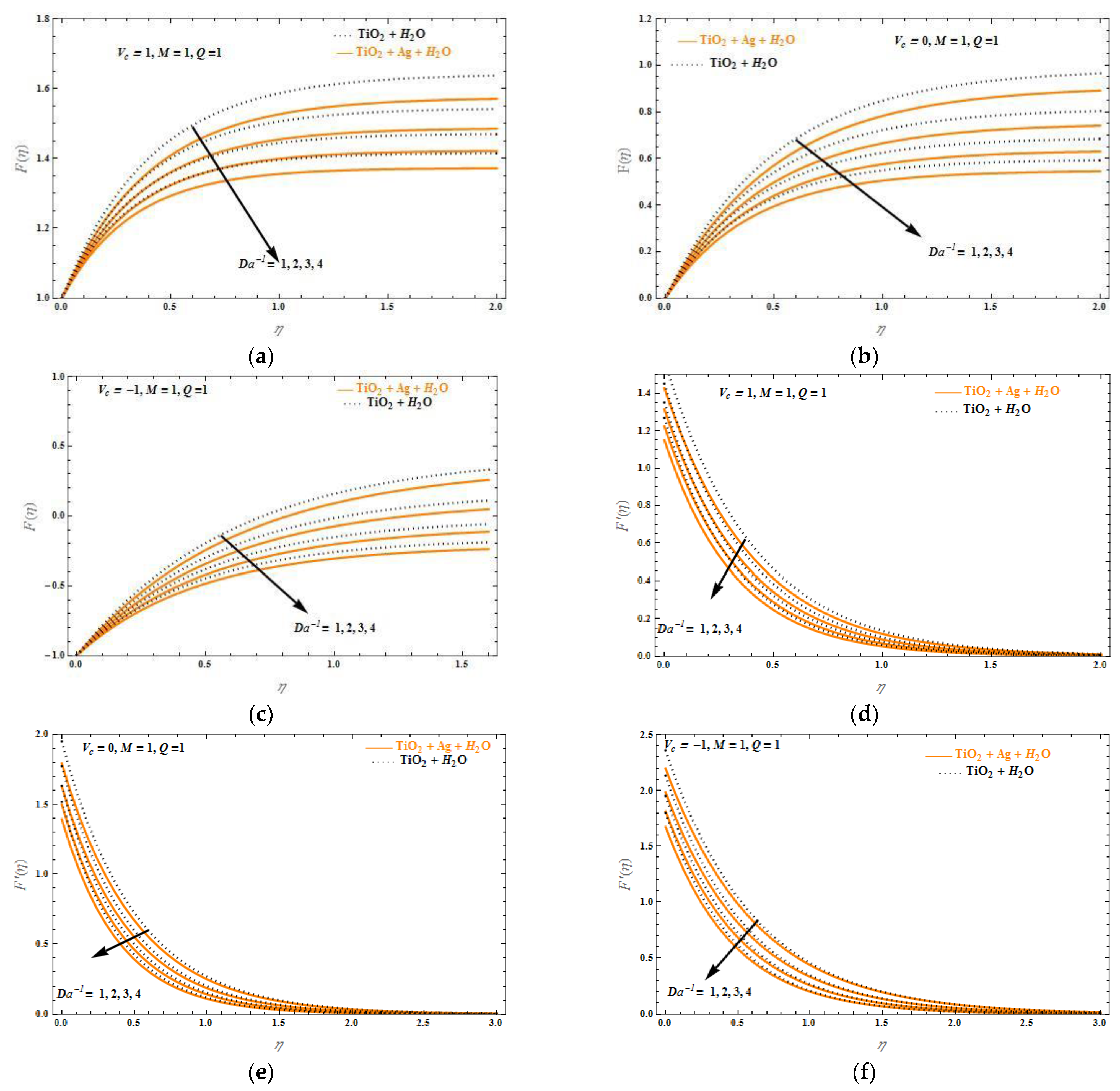
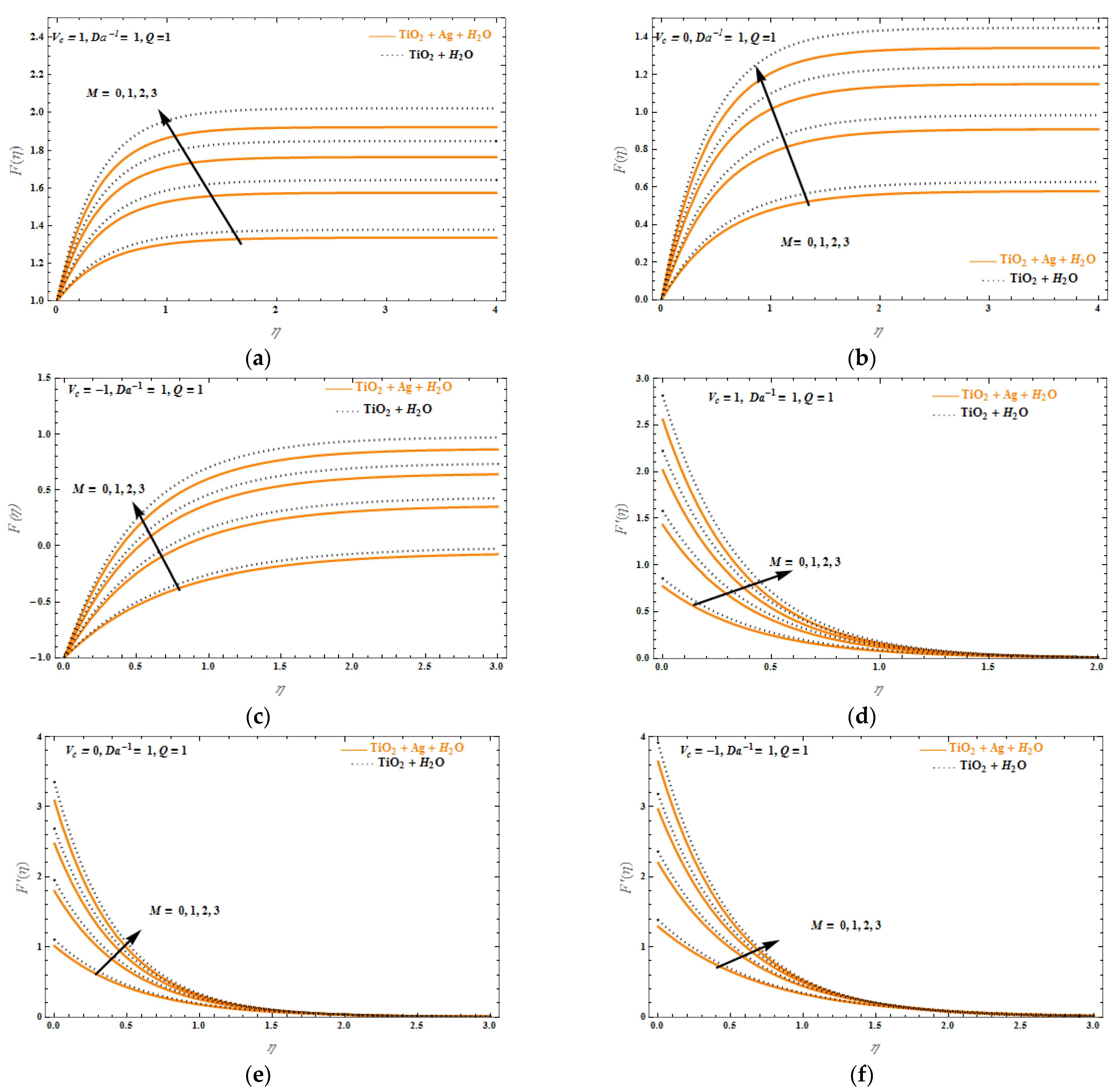
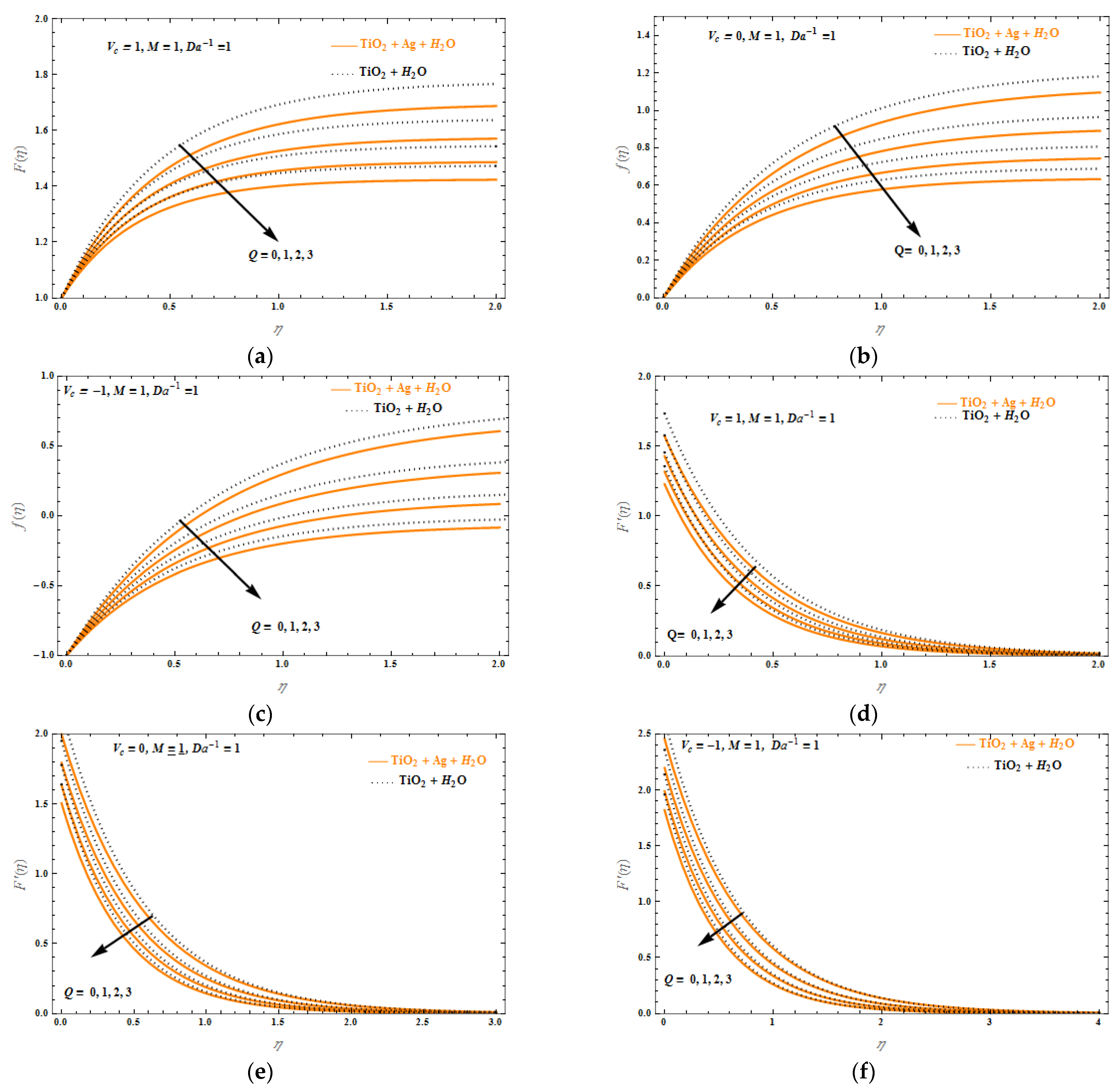
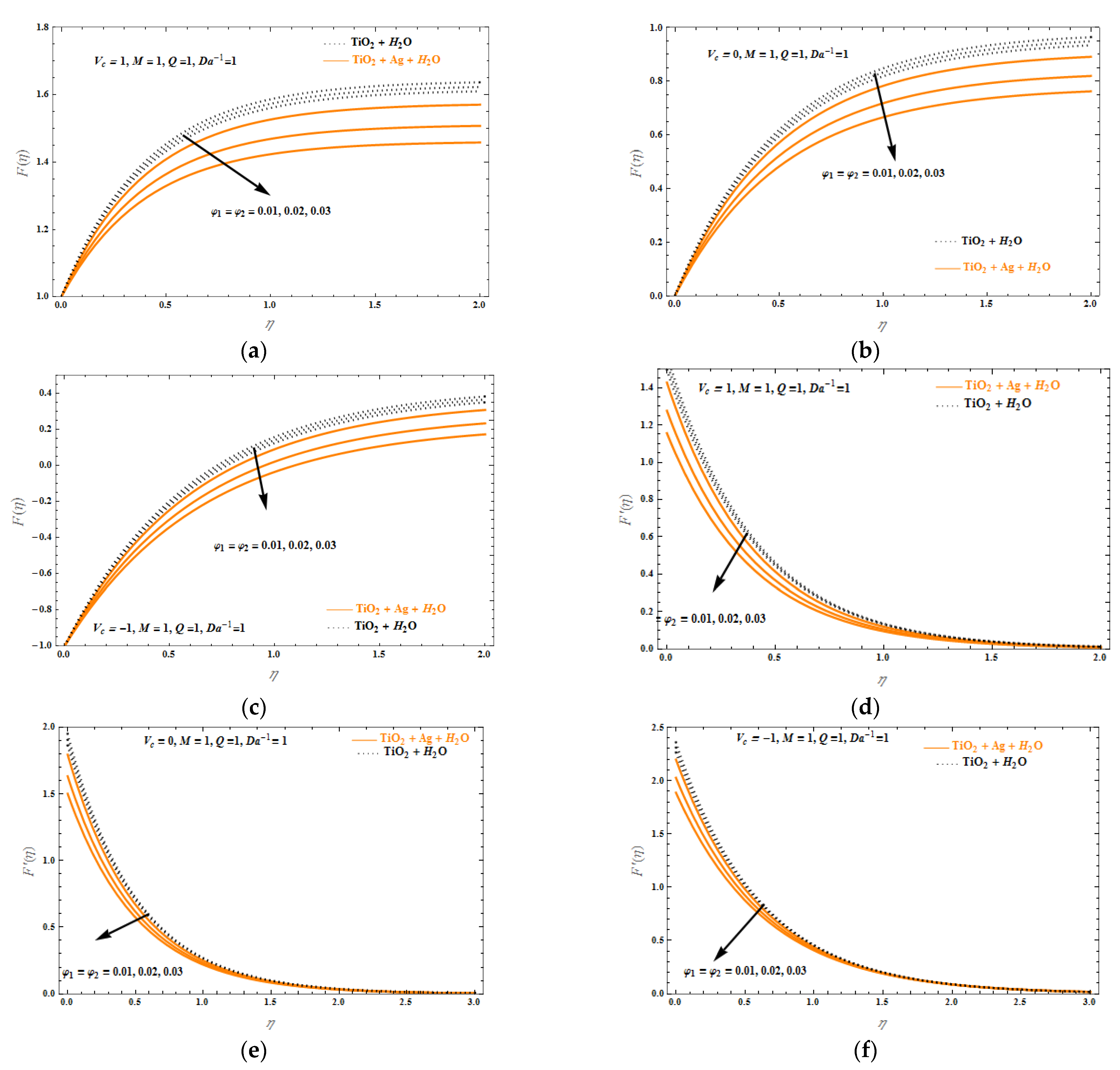
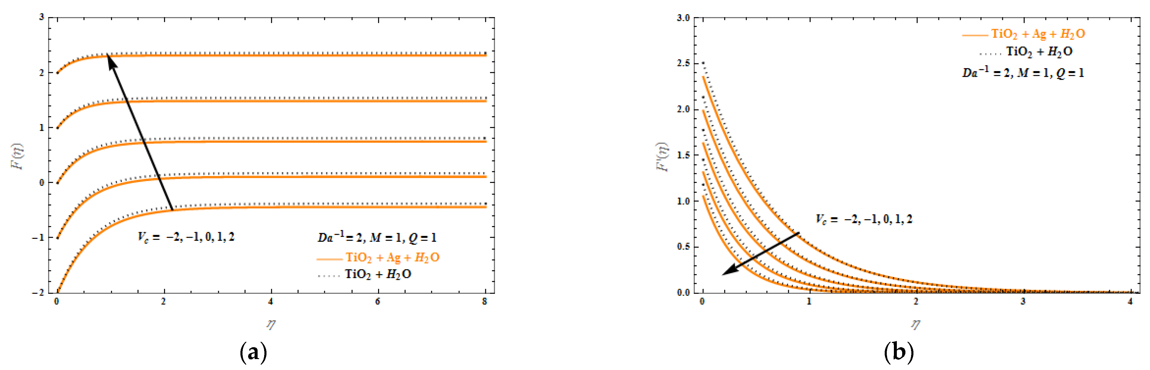
3.1. Velocity Profiles

Figure 2a–f present the physical flow of the problem, which depends on the choice of M (Equation (21)), with both positive and negative solutions The physical solution varies in accordance with variations in the Marangoni number M. Solid lines (green, orange, and black) refer to the (TiO2-Ag, H2O) solution, while dotted lines (green, orange, and black) refer to the (TiO2, H2O) solution. In Figure 2a–c, one observes that the physical solutions are obtained for a 1 and a 2 roots and non-physical solutions are obtained for a 3 roots. Furthermore, the physical solutions are directly affected by V c values. When porosity D a 1 increases from 0 to 5, one observes that at V c = 1 (Figure 2a—suction case) the physical flow solutions show that the (TiO2-Ag, H20) HNF presents higher velocity values compared to the (TiO2, H2O). At V c = 0 (Figure 2b—impermeable case), the physical flow solutions of (TiO2-Ag, H2O) and (TiO2, H2O) HNF are identical. In Figure 2c, at V c = 1 (injection case), the physical flow solutions of the (TiO2, H2O) HNF present higher velocity values compared to the (TiO2-Ag, H2O).
Another parameter of importance is the magnetic field, Q. When porosity D a 1 = 0 and Q increases from 1 to 5, one observes that at V c = 1 (Figure 2d—suction case) we obtain higher velocities for (TiO2-Ag, H2O) compared to (TiO2, H2O); in Figure 2e for V c = 0 (impermeably case), the physical flow solutions of (TiO2-Ag, H2O) are similar to (TiO2, H2O), while in Figure 2f, for V c = 1 (injection case) we obtain smaller velocities for (TiO2-Ag, H2O) compared to (TiO2, H2O).
Figure 3a–f depict the connection between the surface velocity F ( 0 ) (which is connected to the roots a 1 a 2 a 3 ) to M. Following similar color coding as in Figure 2, F ( 0 ) is shown for various values of the parameters Vc, D a 1 , and Q. The range of physical and non-physical surface velocity corresponds to the positive and negative roots, respectively. Let us point out that the physical solutions are obtained for a 1 and a 2 roots and non-physical solutions are obtained for the a 3 root in Figure 3a–c. While the porosity number D a 1   increases from 2 to 5 and Q = 1, it is observed that for all three cases of mass transpiration ( V c = 1 , suction, V c = 0 , impermeable, V c = 1 , injection), the physical flow solutions for the (TiO2, H2O) mixture lead to an increase in surface velocity compared to the (TiO2-Ag, H2O) HNF. By increasing the magnetic field Q from 1 to 2, in Figure 4d–f, we observe that the surface velocity is higher for the (TiO2, H2O) compared to the (TiO2-Ag, H2O) for all three V c cases.
Further investigation is shed on the estimation of the transverse F ( η ) and axial F ( η ) velocity boundaries for the three scenarios of wall mass transfer parameter V c (suction, impermeable and injection) along with the effect of D a 1 , Q, and M, in Figure 4a–f. A common trend in all plots is that the velocity and boundary layer thickness of the fluid is decreased when D a 1 increases from 1 to 4, as well as when the value of V c decreases. This is because by increasing the value of D a 1 , this means that there is also a rise in the holes of the porous structure, and this, in turn, decreases fluid flow. Another common characteristic of Figure 4a–f is that higher velocity values are given for the (TiO2, H2O) compared to the (TiO2-Ag, H2O) HNF. We attribute this behavior to the higher density of the (TiO2-Ag, H2O) HNF, which imposes obstacles in fluid motion, compared to the lower density mixture of (TiO2, H2O).
From another perspective, we argue for the effect of M on F ( η ) and F ( η ) in Figure 5a–f. For all cases investigated, higher axial and transverse velocities are obtained when M increases, and this increase is always higher when the fluid mixture is (TiO2, H2O) compared to (TiO2-Ag, H2O).
The detailed effect of Q on F ( η ) and F ( η ) is depicted in Figure 6a–f. By increasing the magnetic field parameter Q from 0 to 3, the application of a normal magnetic field to an electrically conducting fluid produces a drag-like force known as the Lorentz force, which operates in the opposite direction of the flow, resulting in flow retardation. This fact reduces the fluid and boundary layer velocity values. Furthermore, there are higher velocities for (TiO2, H2O) compared to (TiO2-Ag, H2O).
Let us now turn to the effect of the solid volume fraction of nanoparticles in the fluid mixture in Figure 7a–f. We denote as φ1 the volume fraction of TiO2 and as φ2 the volume fraction of Ag nanoparticles. It is noted that by increasing φ1 and φ2 at the same time, the velocity values of (TiO2-Ag, H2O) are decreased in the respective fluid mixtures. By only increasing the value φ1, the velocity values of (TiO2, H2O) are decreased in the respective fluid mixtures. As also shown in previous cases (Figure 3, Figure 4, Figure 5 and Figure 6), higher velocities are observed for (TiO2, H2O) compared to (TiO2-Ag, H2O).
The effect of V c on the axial and transverse velocity profiles is shown in Figure 8. As the mass transpiration increases in the range 2 V c 2 , F(n) increases, while F ( n ) decreases.

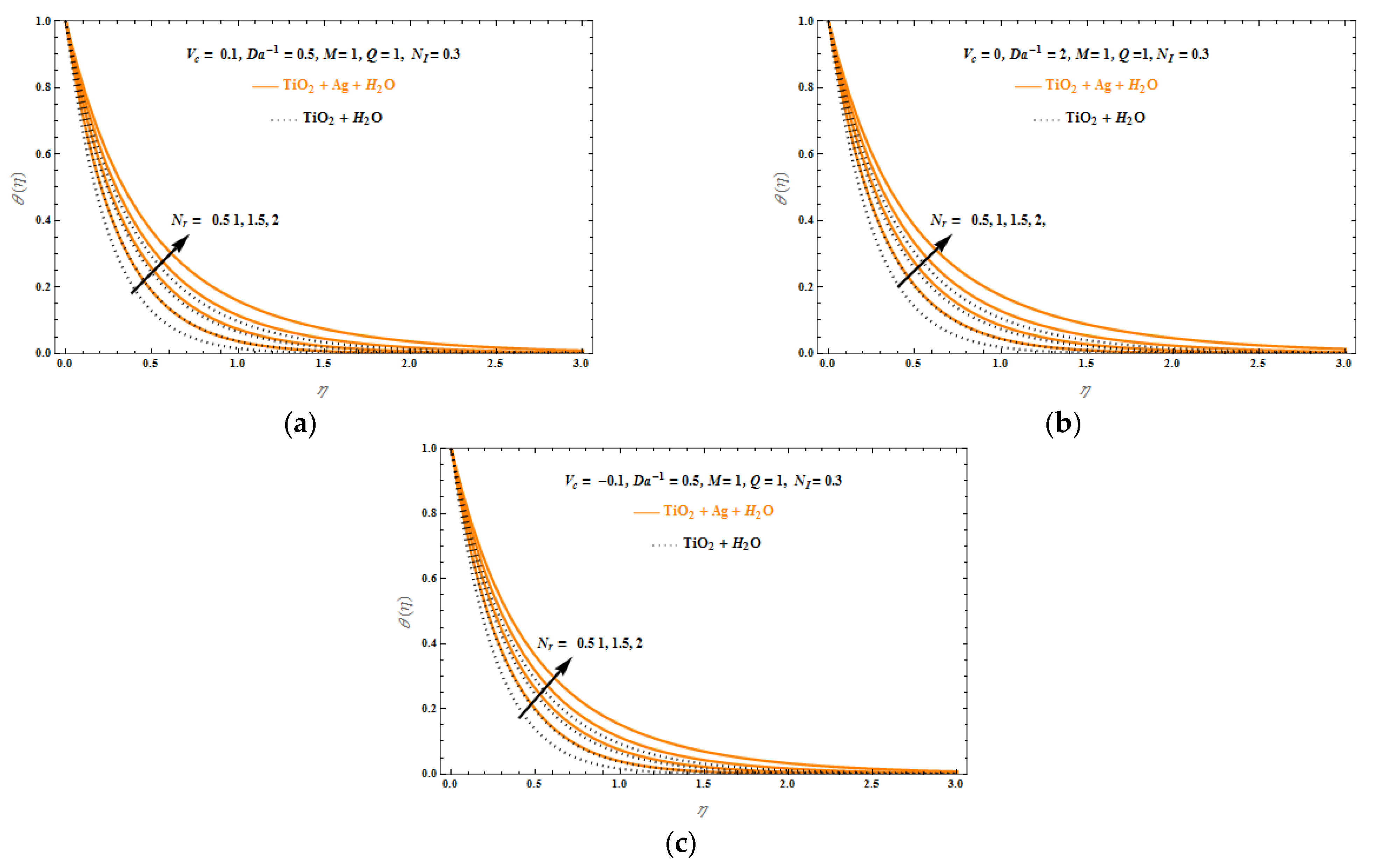
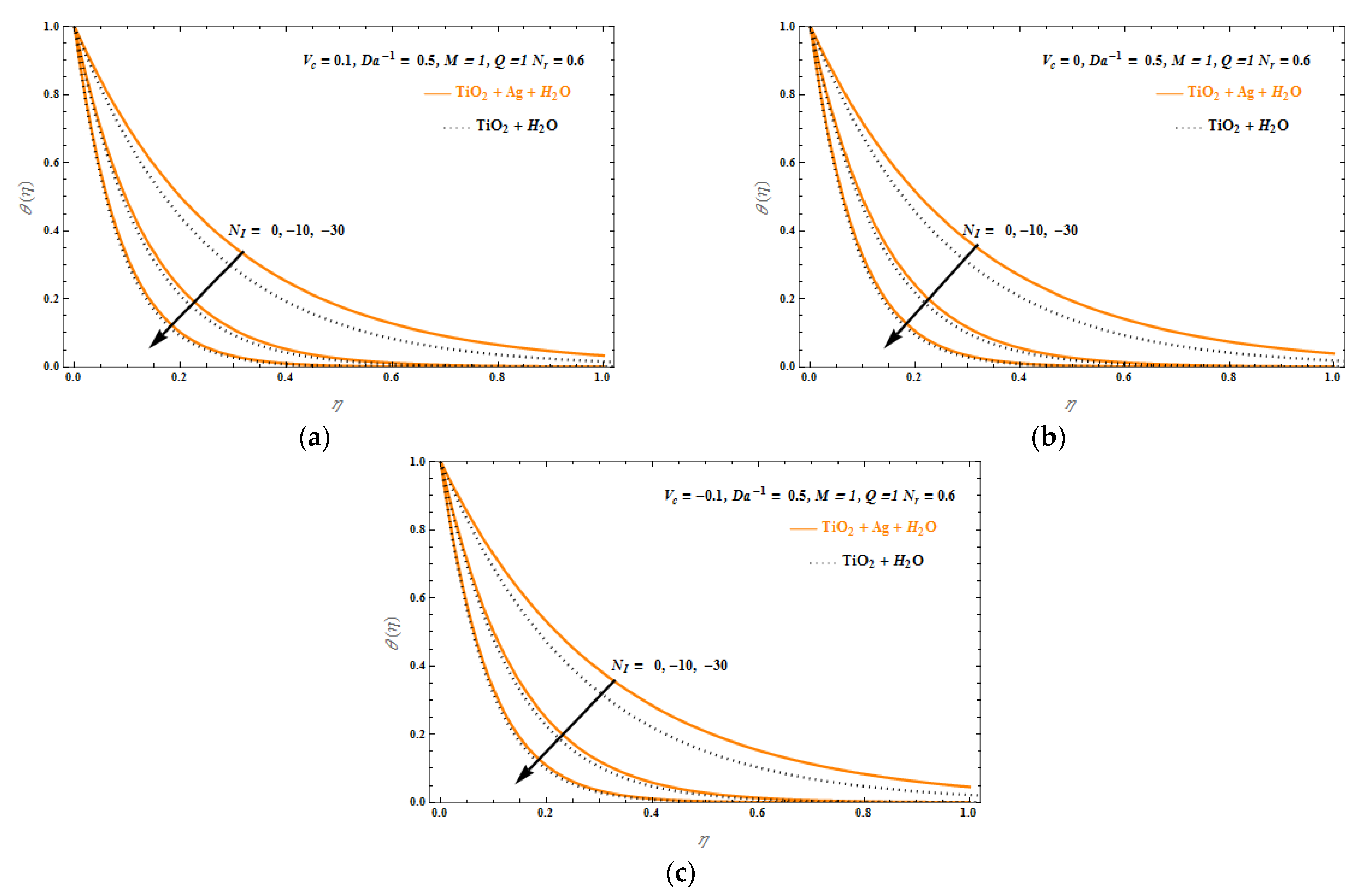
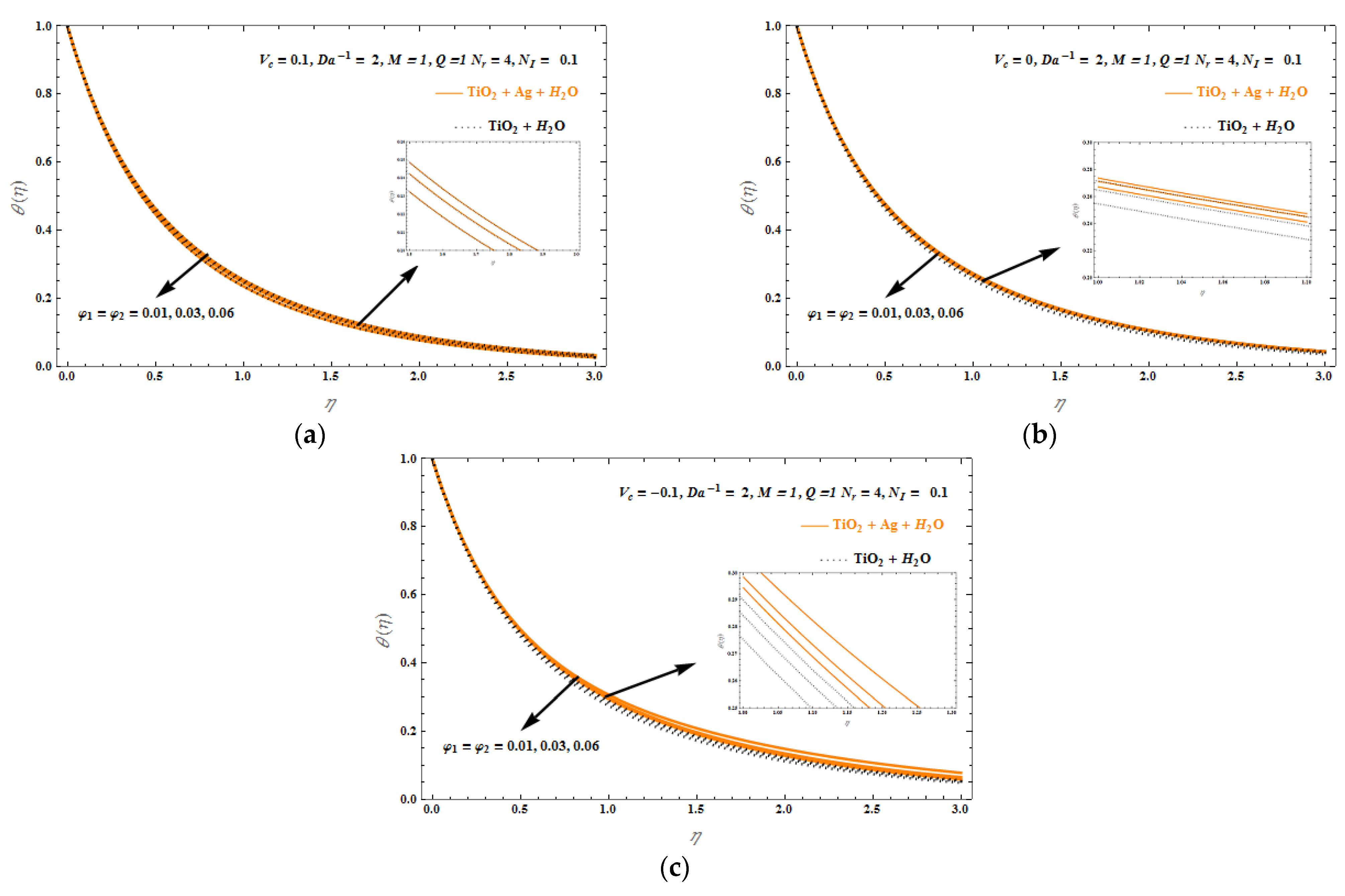
3.2. Temperature Profiles

The effects of thermal radiation ( N r ) , heat source and sink ( N I ) , inverse Darcy number ( D a 1 ) and solid volume fraction of TiO2 and Ag in water solution ( φ 1 , φ 2 ) are investigated next. Starting from the N r effect, as it increases in the range {0.5, 1.0, 1.5, 2.0}, in Figure 9a–c, one obtains greater thickness in the thermal boundary. As long as the N I effect is concerned, as it decreases in the range N I = 0 , 10 , 30 , in Figure 10a–c, there is decreasing thickness in the thermal boundary layer. The thermal boundary layer increases when D a 1 increases (Figure 11a–c). Finally, in Figure 12a–c, one observes that the thermal boundary layer increases while increasing the volume fraction of TiO2 and Ag.
The main outcome of all temperature profiles shown here is that, as temperature is higher for (TiO2-Ag, H2O) compared to (TiO2, H2O), the mixing of two nanoparticles TiO2 and Ag in H2O results in greater heat energy than the single nanoparticle TiO2 in H2O.

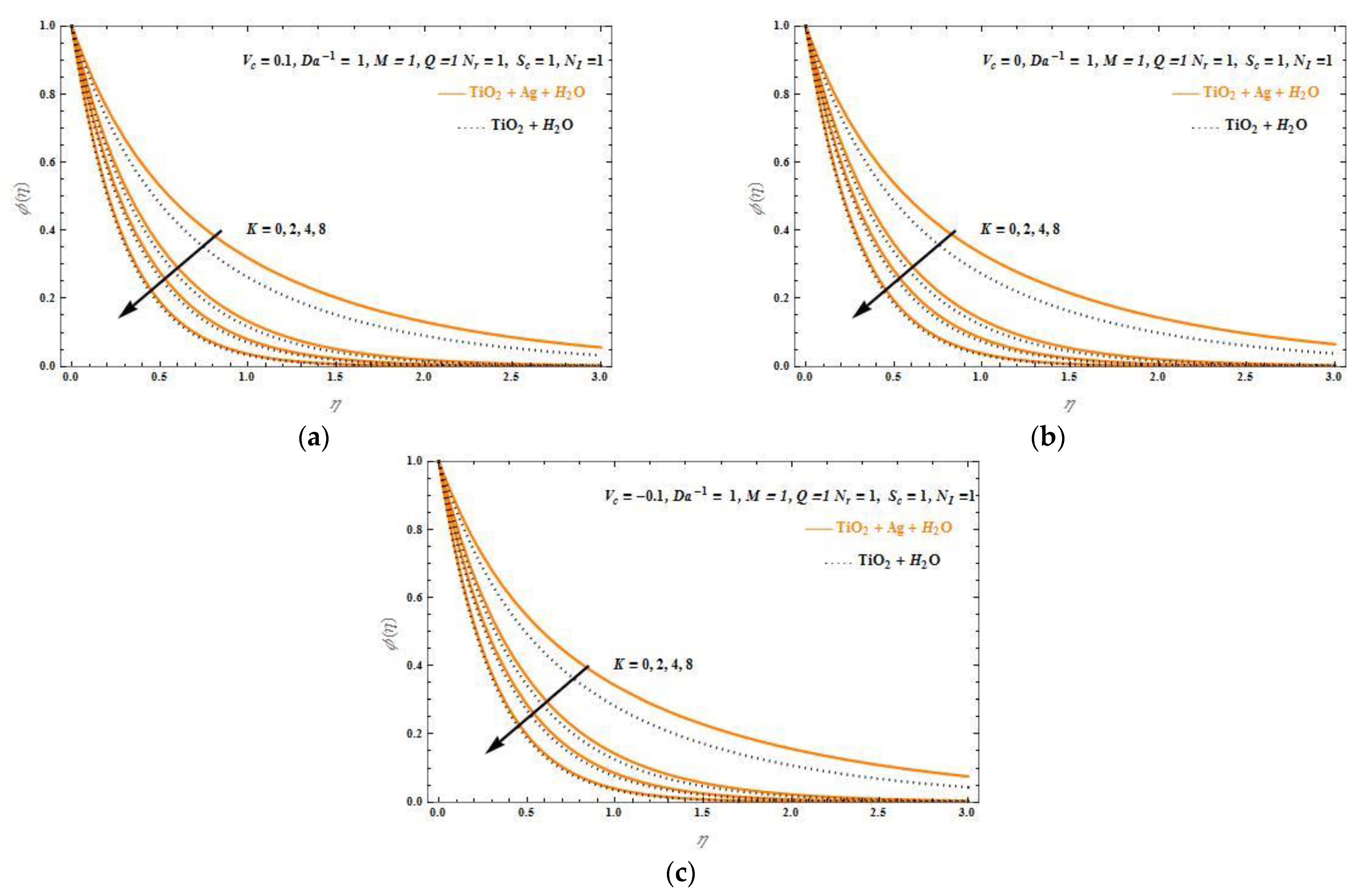
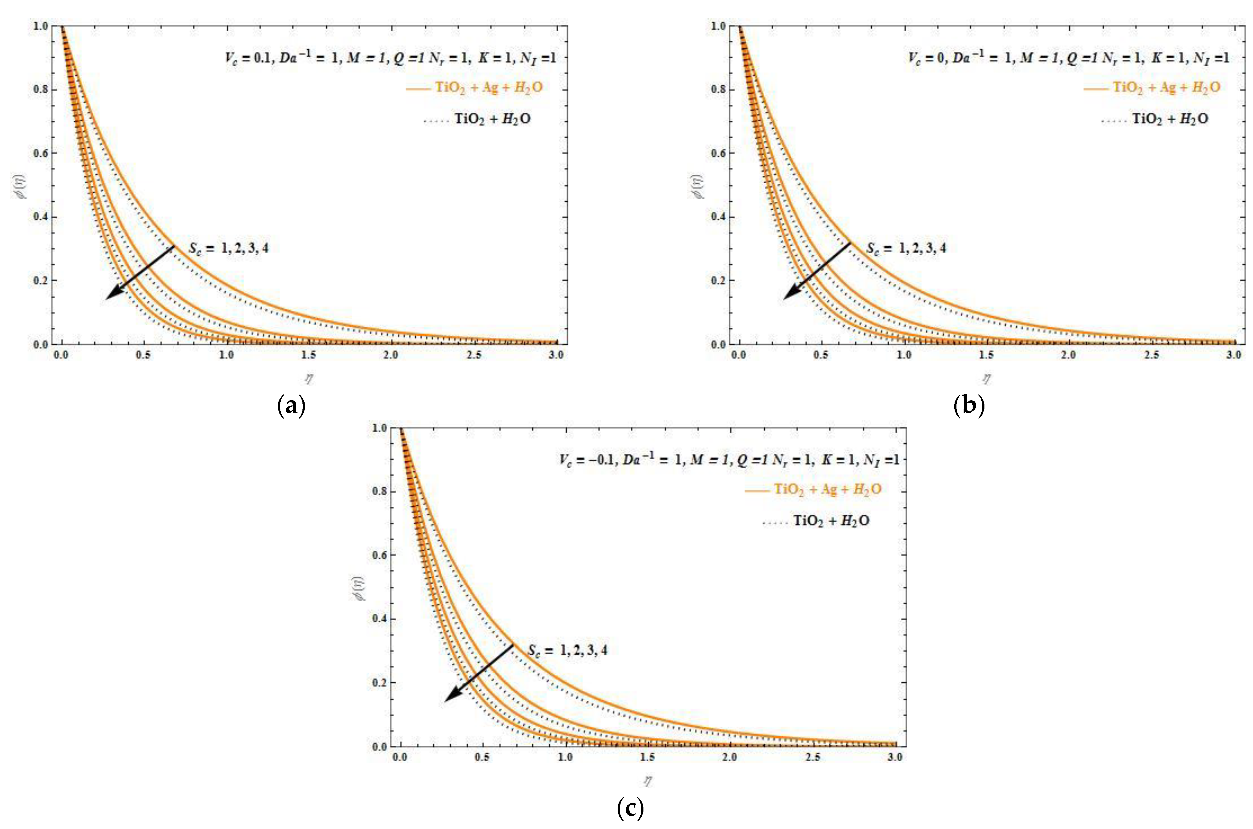
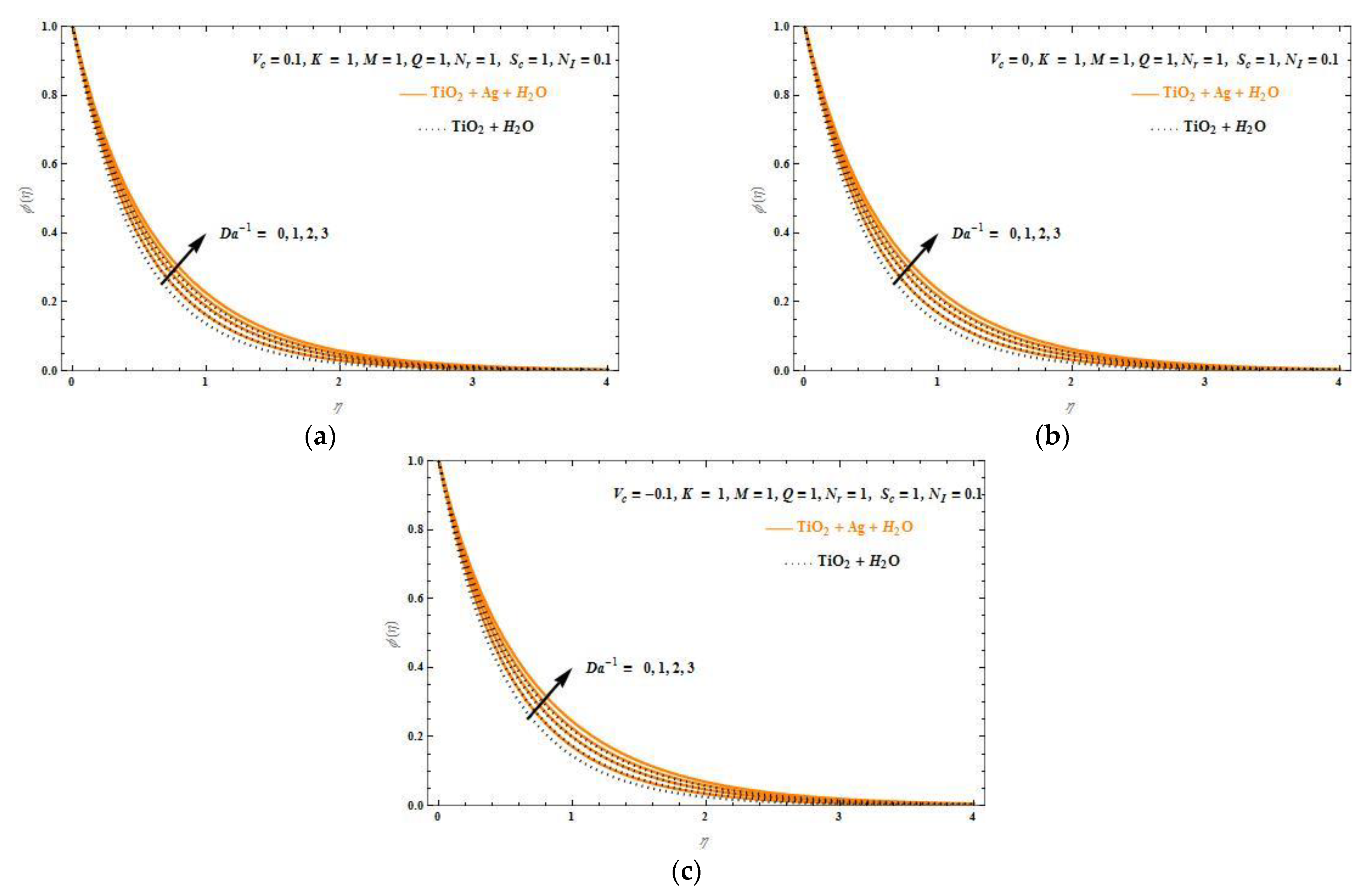
3.3. Concentration Profiles

The effects of the chemical reaction coefficient, K , Schmidt number, S c , the inverse Darcy number, D a 1 , are investigated next, in Figure 13, Figure 14 and Figure 15, for the three cases of mass transpiration (suction, impermeable, and injection), in order to present concentration profiles for the problem and argue on the chemical boundary thickness. First, consider K = {0,2,4,8}, in Figure 13a–c. As K increases, the chemical boundary layer thickness decreases, and the fluid force moves near the surface. Similar behavior is observed as S c increases in the range S c   = {1,2,3,4}, in Figure 14a–c. On the opposite, as D a 1 increases, one obtains greater chemical boundary layer thickness values (Figure 15a–c).
The common outcome of the concentration profiles shown here is that all profiles for the (TiO2-Ag, H2O) mixture present higher values compared to the (TiO2, H2O) mixture, and this is evidence that the mixing of two nanoparticles TiO2 and Ag in H2O results in greater chemical energy than the single nanoparticle TiO2 in H2O.

3.4. Validation

The research has revealed that the mixture of TiO2 –Ag with H2O gives higher heat energy compared to the mixture of only TiO2 with H2O for Newtonian radiative flow at the thermosolutal Marangoni boundary over a porous medium, under the effect of magnetic field and mass transpiration in fluid velocity, and obtained an exact analytical solution in terms of hypergeometric functions. In the absence of the HNF and Q = 0 ,   D a 1 = 0 , this agrees to the results obtained by Magyari et al. [8]. When Q = 0 , the absence of HNF leads to the results of Mahabaleshwar et al. [9], while, when also considering the unsteady case, the results agree to the results by Hassan [10]. The results of all these studies along with the results of the present paper are summarized in Table 3.

4. Conclusions

This study has presented in detail the effect of mass transpiration generated by a hybrid nanofluid under the effect of chemically radiative TS-MC fluid flow in porous media in the presence of heat sources/sinks and a magnetic field. This is a multiparametric problem that takes into account the effect of various parameters, such as the Marangoni number, M, mass transpiration, Vc, thermal radiation, N r , heat source and sink, N I , the inverse Darcy number, D a 1 , the volume fraction of nanoparticles in water, φ 1 , φ 2 , the magnetic field, Q, the chemical reaction coefficient, K , and Schmidt number, S c .
The exact analytical solutions are produced by using the Cardon’s method and confluent hypergeometric functions, and profiles for properties of interest are shown (velocity, temperature and concentration). The main outcomes of the study are as follows:
  • the physical solution’s effect is directly determined by Vc, D a 1 , and Q;
  • Vc has a direct impact on surface velocity and Marangoni number, M;
  • by increasing the values of the magnetic field, Q, and porosity, D a 1 , the fluid velocity decreases;
  • on the other hand, by increasing the Marangoni number, M, the fluid velocity increases;
  • the velocity and thermal boundary layer decrease by increasing the volume fraction of TiO2 and Ag within H2O;
  • furthermore, the (TiO2, H2O) mixture presents higher velocity values, but less heat and chemical energy compared to the (TiO2-Ag, H2O);
  • the thermal boundary layers increase when N r increases and decrease when N I increases;
  • the thermal and chemical boundary layers increase by increasing the value of D a 1 ;
  • the concentration profile decreases when Sc and K increase.
In future, we plan to perform a similar investigation on non-Newtonian fluids and a ternary nanofluid with the effect of slip condition in a porous medium.

Author Contributions

Conceptualization: U.S.M.; methodology: U.S.M. and F.S.; software: R.M. and U.S.M.; formal analysis: F.S., R.M. and U.S.M.; investigation: R.M., U.S.M. and F.S.; writing—original draft preparation: U.S.M.; writing—review and editing: F.S. All authors have read and agreed to the published version of the manuscript.

Funding

F.S. acknowledges support from the project CAMINOS, which is implemented in the context of a grant by the Center of Research Innovation and Excellence of University of Thessaly (Lamia, Greece), funded by the Special Account for Research Grants of University of Thessaly.

Data Availability Statement

Not applicable.

Conflicts of Interest

The authors declare no conflict of interest.

Nomenclature

Latin symbols
A 1 , A 2 , A 3 , A 4 , A 5 constants
B 0 applied magnetic field
C dimensional concentration
C P specific heat, constant pressure
D Mass diffusivity
D 1 , D 2 constants
D a 1 inverse Darcy number
F velocity similarity
F Constant
F ( η ) axial   velocity  
F ( η ) transverse velocity
H confluent hypergeometric function
k permeability
Kchemical reaction coefficient
L characteristic/reference length
MMarangoni number
m , n constants
N r radiation parameter
N I heat source and sink parameter
PrPrandtl number
q r radiative heat flux
q w local heat flux at the wall
Qmagnetic field
S 1 , S 2 constants
S c Schmidt number
Ttemperature
T0constant
V c mass transformation
V c > 0 suction condition
V c = 0 impermeability condition
V c < 0 injection condition
( x , y ) axes
( u , v ) velocities along x- and y-directions
Greek symbols
α thermal diffusivity
γ coefficient
Δ discriminates
ηsimilarity variable
κ thermal conductivity
μ f dynamic viscosity
ν kinematic viscosity
ρ density
σ electrical conductivity
σ 1 surface tension
σ 0 equilibrium surface tension
σ s 1 ,   σ s 2 electrical conductivities, respectively, of TiO2 and Ag nanoparticles
σ * Stefan-Boltzmann constant
φ 1 , φ 2 nanoparticle volume fractions of TiO2 and Ag, respectively
ϕ concentration similarity variable
ψ stream function
Subscripts
C solutal quantity
T thermal quantity
b f base fluid
n f Nanofluid
h n f hybrid nanofluid
f ,   f ,   f First, second and third order derivatives with respect to η
Abbreviations
Agsilver
BCboundary condition
BLFboundary layer flow
CNTcarbon nanotube
EHDelectrohydrodynamics
H2Owater
HNFhybrid nanofluid
MCMarangoni convection
MHDmagnetohydrodynamics
ODEordinary differential equation
PDEpartial differantial equation
TiO2titanium dioxide
TSthermosolutal

References

  1. Ahmed, S.E.; Oztop, H.F.; Elshehabey, H.M. Thermosolutal Marangoni Convection of Bingham Non-Newtonian Fluids within Inclined Lid-Driven Enclosures Full of Porous Media. Heat Transfer 2021, 50, 7898–7917. [Google Scholar] [CrossRef]
  2. Qayyum, S. Dynamics of Marangoni Convection in Hybrid Nanofluid Flow Submerged in Ethylene Glycol and Water Base Fluids. Int. Comm. Heat Mass Transfer 2020, 119, 104962. [Google Scholar] [CrossRef]
  3. Butzhammer, L.; Köhler, W. Thermocapillary and Thermosolutal Marangoni Convection of Ethanol and Ethanol–Water Mixtures in a Microfluidic Device. Microfl. Nanofl. 2017, 21, 155. [Google Scholar] [CrossRef]
  4. Napolitano, L.G. Marangoni Boundary Layers. In Proceedings of the 3rd European Symposium on Materials Sciences in Space, Grenoble, France, 24–27 April 1979; pp. 349–358. [Google Scholar]
  5. Napolitano, L.G. Microgravity Fluid Dynamics. In Proceedings of the 2nd Levitch Conference, Washington, DC, USA, November 1978. [Google Scholar]
  6. Pop, I.; Postelnicu, A.; Groşan, T. Thermosolutal Marangoni Forced Convection Boundary Layers. Meccanica 2001, 36, 555–571. [Google Scholar] [CrossRef]
  7. Al-Mudhaf, A.; Chamkha, A.J. Similarity Solutions for MHD Thermosolutal Marangoni Convection over a Flat Surface in the Presence of Heat Generation or Absorption Effects. Heat Mass Transfer 2005, 42, 112–121. [Google Scholar] [CrossRef]
  8. Magyari, E.; Chamkha, A.J. Exact Analytical Solutions for Thermosolutal Marangoni Convection in the Presence of Heat and Mass Generation or Consumption. Heat Mass Transfer 2007, 43, 965–974. [Google Scholar] [CrossRef] [Green Version]
  9. Mahabaleshwar, U.S.; Nagaraju, K.R.; Vinay Kumar, P.N.; Azese, M.N. Effect of Radiation on Thermosolutal Marangoni Convection in a Porous Medium with Chemical Reaction and Heat Source/Sink. Phys. Fluids 2020, 32, 113602. [Google Scholar] [CrossRef]
  10. Hassan, M. Thermosolutal Marangoni Convection Effect on the MHD Flow over an Unsteady Stretching Sheet. J. Egypt. Math. Soc. 2018, 26, 58–71. [Google Scholar] [CrossRef]
  11. Mackolil, J.; Mahanthesh, B. Heat Transfer Optimization and Sensitivity Analysis of Marangoni Convection in Nanoliquid with Nanoparticle Interfacial Layer and Cross-Diffusion Effects. Int. Comm. Heat Mass Transfer 2021, 126, 105361. [Google Scholar] [CrossRef]
  12. Patil, P.M.; Kulkarni, M. Analysis of MHD Mixed Convection in a Ag-TiO2 Hybrid Nanofluid Flow Past a Slender Cylinder. Chin. J. Phys. 2021, 73, 406–419. [Google Scholar] [CrossRef]
  13. Shoaib, M.; Tabassum, R.; Nisar, K.S.; Raja, M.A.Z.; Rafiq, A.; Khan, M.I.; Jamshed, W.; Abdel-Aty, A.-H.; Yahia, I.S.; Mahmoud, E.E. Entropy Optimized Second Grade Fluid with MHD and Marangoni Convection Impacts: An Intelligent Neuro-Computing Paradigm. Coatings 2021, 11, 1492. [Google Scholar] [CrossRef]
  14. Ullah, I. Heat Transfer Enhancement in Marangoni Convection and Nonlinear Radiative Flow of Gasoline Oil Conveying Boehmite Alumina and Aluminum Alloy Nanoparticles. Int. Comm. Heat Mass Transfer 2022, 132, 105920. [Google Scholar] [CrossRef]
  15. Suresh, S.; Venkitaraj, K.P.; Selvakumar, P.; Chandrasekar, M. Synthesis of Al2O3–Cu/Water Hybrid Nanofluids Using Two Step Method and Its Thermo Physical Properties. Colloid. Surf. A: Physicochem. Eng. Aspects 2011, 388, 41–48. [Google Scholar] [CrossRef]
  16. Choi, S.U.S.; Eastman, J.A. Enhancing Thermal Conductivity of Fluids with Nanoparticles. In Proceedings of the ASME International Mechanical Engineering Congress and Exhibition, San Francisco, CA, USA, 12–17 November 1995; Available online: https://digital.library.unt.edu/ark:/67531/metadc671104/ (accessed on 15 December 2022).
  17. Zhuang, Y.J.; Zhu, Q.Y. Numerical Study on Combined Buoyancy–Marangoni Convection Heat and Mass Transfer of Power-Law Nanofluids in a Cubic Cavity Filled with a Heterogeneous Porous Medium. Int. J. Heat Fluid Flow 2018, 71, 39–54. [Google Scholar] [CrossRef]
  18. Kasaeian, A.; Daneshazarian, R.; Mahian, O.; Kolsi, L.; Chamkha, A.J.; Wongwises, S.; Pop, I. Nanofluid Flow and Heat Transfer in Porous Media: A Review of the Latest Developments. Int. J. Heat Mass Transfer 2017, 107, 778–791. [Google Scholar] [CrossRef]
  19. Tripathi, R. Marangoni Convection in the Transient Flow of Hybrid Nanoliquid Thin Film over a Radially Stretching Disk. Proc. Inst. Mech. Eng. E: J. Proc. Mech. Eng. 2021, 235, 800–811. [Google Scholar] [CrossRef]
  20. Li, Y.-X.; Khan, M.I.; Gowda, R.J.P.; Ali, A.; Farooq, S.; Chu, Y.-M.; Khan, S.U. Dynamics of Aluminum Oxide and Copper Hybrid Nanofluid in Nonlinear Mixed Marangoni Convective Flow with Entropy Generation: Applications to Renewable Energy. Chin. J. Phys. 2021, 73, 275–287. [Google Scholar] [CrossRef]
  21. Jawad, M.; Saeed, A.; Tassaddiq, A.; Khan, A.; Gul, T.; Kumam, P.; Shah, Z. Insight into the Dynamics of Second Grade Hybrid Radiative Nanofluid Flow within the Boundary Layer Subject to Lorentz Force. Sci. Rep. 2021, 11, 4894. [Google Scholar] [CrossRef]
  22. Forchheimer, P. Wasserbewegung durch Boden. Z. Ver. Deutsch. Ing. 1901, 45, 1782–1788. [Google Scholar]
  23. Muskat, M. The Flow of Homogeneous Fluids through Porous Media; McGraw-Hill Book Company: New York, NY, USA, 1937; Available online: https://blasingame.engr.tamu.edu/z_zCourse_Archive/P620_18C/P620_zReference/PDF_Txt_Msk_Flw_Fld_(1946).pdf (accessed on 15 December 2022).
  24. Hayat, T.; Haider, F.; Muhammad, T.; Alsaedi, A. On Darcy-Forchheimer Flow of Carbon Nanotubes due to a Rotating Disk. Int. J. Heat Mass Transfer 2017, 112, 248–254. [Google Scholar] [CrossRef]
  25. Vishnu Ganesh, N.; Abdul Hakeem, A.K.; Ganga, B. Darcy–Forchheimer Flow of Hydromagnetic Nanofluid Over a Stretching/Shrinking Sheet in a Thermally Stratified Porous Medium with Second Order Slip, Viscous and Ohmic Dissipations Effects. Ain Shams Eng. J. 2018, 9, 939–951. [Google Scholar] [CrossRef]
  26. Muhammad, T.; Alsaedi, A.; Shehzad, A.S.; Hayat, T. A Revised Model for Darcy-Forchheimer Flow of Maxwell Nanofluid Subject to Convective Boundary Condition. Chin. J. Phys. 2017, 55, 963–976. [Google Scholar] [CrossRef]
  27. Jawad, M.; Saeed, A.; Kumam, P.; Shah, Z.; Khan, A. Analysis of Boundary Layer MHD Darcy-Forchheimer Radiative Nanofluid Flow with Soret and Dufour Effects by Means of Marangoni Convection. Case Stud. Therm. Eng. 2021, 23, 100792. [Google Scholar] [CrossRef]
  28. Moatimid, G.M.; Hassan, M.A. The Instability of an Electrohydrodynamic Viscous Liquid Micro-Cylinder Buried in a Porous Medium: Effect of Thermosolutal Marangoni Convection. Math. Probl. Eng. 2013, 2013, e416562. [Google Scholar] [CrossRef]
  29. Mahdy, A.; Ahmed, S.E. Thermosolutal Marangoni Boundary Layer Magnetohydrodynamic Flow with the Soret and Dufour Effects Past a Vertical Flat Plate. Eng. Sci. Tech. Int. J. 2015, 18, 24–31. [Google Scholar] [CrossRef] [Green Version]
  30. Siddheshwar, P.G.; Mahabaleswar, U.S. Effects of Radiation and Heat Source on MHD Flow of a Viscoelastic Liquid and Heat Transfer over a Stretching Sheet. Int. J. Non-Lin. Mech. 2005, 40, 807–820. [Google Scholar] [CrossRef] [Green Version]
  31. Mahanthesh, B.; Gireesha, B.J. Thermal Marangoni Convection in Two-Phase Flow of Dusty Casson Fluid. Results Phys. 2018, 8, 537–544. [Google Scholar] [CrossRef]
  32. Lin, Y.; Zheng, L.; Zhang, X. Radiation Effects on Marangoni Convection Flow and Heat Transfer in Pseudo-Plastic Non-Newtonian Nanofluids with Variable Thermal Conductivity. Int. J. Heat Mass Transfer 2014, 77, 708–716. [Google Scholar] [CrossRef]
  33. Patil, P.M.; Pop, I. Effects of Surface Mass Transfer on Unsteady Mixed Convection Flow over a Vertical Cone with Chemical Reaction. Heat Mass Transfer 2011, 47, 1453–1464. [Google Scholar] [CrossRef]
  34. Li, B.; Zheng, L.; Zhang, X. Comparison Between Thermal Conductivity Models on Heat Transfer in Power-Law Non-Newtonian Fluids. J. Heat Transfer 2012, 134, 041702. [Google Scholar] [CrossRef]
  35. Hayat, T.; Khan, M.I.; Farooq, M.; Alsaedi, A.; Yasmeen, T. Impact of Marangoni Convection in the Flow of Carbon–Water Nanofluid with Thermal Radiation. Int. J. Heat Mass Transfer 2017, 106, 810–815. [Google Scholar] [CrossRef]
  36. Khan, U.; Zaib, A.; Ishak, A.; Roy, N.C.; Bakar, S.A.; Muhammad, T.; Abdel-Aty, A.-H.; Yahia, I.S. Exact Solutions for MHD Axisymmetric Hybrid Nanofluid Flow and Heat Transfer over a Permeable Non-Linear Radially Shrinking/Stretching Surface with Mutual Impacts of Thermal Radiation. Eur. Phys. J. Spec. Top. 2022, 231, 1195–1204. [Google Scholar] [CrossRef]
  37. Anusha, T.; Huang, H.-N.; Mahabaleshwar, U.S. Two Dimensional Unsteady Stagnation Point Flow of Casson Hybrid Nanofluid over a Permeable Flat Surface and Heat Transfer Analysis with Radiation. J. Taiwan Inst. Chem. Eng. 2021, 127, 79–91. [Google Scholar] [CrossRef]
  38. Sneha, K.N.; Mahabaleshwar, U.S.; Chan, A.; Hatami, M. Investigation of Radiation and MHD on Non-Newtonian Fluid Flow over a Stretching/Shrinking Sheet with CNTs and Mass Transpiration. Waves Rand. Compl. Media 2022, 1–20. [Google Scholar] [CrossRef]
Figure 1. The mathematical model of HNF with boundary condition. Concentration, C, velocity, V, and temperature, T, profiles in (x-y) space. B0 is the magnetic field with the direction shown by arrows.
Physics 05 00003 g001
Figure 2. The behavior of the roots a 1 , a 2 , and   a 3 versus Marangoni number, M, and various values for the inverse Darcy number, Da−1, mass transpiration parameter, Vc, and magnetic field, Q. (a) Vc = 1, Q = 1, and Da−1 = 1 and 5; (b) Vc = 0, Q = 1, and Da−1 = 0 and 5; (c) Vc = −1, Q = 1, and Da−1 = 0 and 5; (d) Vc = 1, Q = 1 and 5, and Da−1 = 0; (e) Vc = 0, Q = 1 and 5, and Da−1 = 0; (f) Vc = −1, Q = 1 and 5, and Da−1 = 0.
Physics 05 00003 g002aPhysics 05 00003 g002b
Figure 3. The behavior of similar surface velocity, F ( 0 ) , versus Marangoni number, M, and various values for the inverse Darcy number, Da−1, magnetic field, Q and mass transpiration parameter, Vc. (a) Vc = 1, Q = 1, Da−1 = 2 and 5, (b) Vc = 0, Q = 1, Da−1 = 2 and 5, (c) Vc = −1, Q = 1, Da−1 = 2 and 5, (d) Vc = 1, Q = 1 and 2, Da−1 = 0, (e) Vc = 0, Q = 1 and 2, Da−1 = 0, and (f) Vc = −1, Q = 1 and 2, Da−1 = 0.
Physics 05 00003 g003
Figure 4. The axial, F ( η ) , and transverse, F ( η ) , velocities versus the similarity variable, η , for various values of Da−1 and Q = M = 1 . (a) F(n), for Vc = 1, (b) F(n), for Vc = 0, (c) F(n), for Vc = −1, (d) F ( n ) , for Vc = 1, (e) F ( n ) , for Vc = 0, and (f) F ( n ) , for Vc = −1. The orange solid line refers to the (TiO2-Ag, H2O) HNF and dotted line to (TiO2, H2O).
Physics 05 00003 g004
Figure 5. The axial, F ( η ) , and transverse, F ( η ) ,   velocities versus the similarity variable, η , for various values of M and Q = D a 1 = 1 . (a) F(n), for Vc = 1, (b) F(n), for Vc = 0, (c) F(n), for Vc = −1, (d) F ( n ) , for Vc = 1, (e) F ( n ) , for Vc = 0, and (f) F ( n ) , for Vc = −1. The orange solid line refers to the (TiO2-Ag, H2O) HNF and dotted line to (TiO2, H2O).
Physics 05 00003 g005
Figure 6. The axial, F ( η ) , and transverse, F ( η ) , velocities versus the similarity variable, η , for various values of Q and M = D a 1 = 1 . (a) F(n), for Vc = 1, (b) F(n), for Vc = 0, (c) F(n), for Vc = −1, (d) F ( n ) , for Vc = 1, (e) F ( n ) , for Vc = 0, and (f) F ( n ) , for Vc = −1. The orange solid line refers to the (TiO2-Ag, H20) HNF and dotted line to (TiO2, H2O).
Physics 05 00003 g006
Figure 7. The axial, F ( η ) , and transverse, F ( η )   , velocities versus the similarity variable, η , for various values of φ1 and φ2 and M = Q = D a 1 = 1 . (a) F(n), for Vc = 1, (b) F(n), for Vc = 0, (c) F(n), for Vc = −1, (d) F ( n ) , for Vc = 1, (e) F ( n ) , for Vc = 0, and (f) F ( n ) , for Vc = −1. The orange solid line refers to the (TiO2-Ag, H2O) HNF and dotted line to (TiO2, H2O).
Physics 05 00003 g007
Figure 8. (a) Axial, F ( η ) , and (b) transverse, F ( η ) , velocities versus the similarity variable, η . M = Q = 1 , D a 1 = 2 . The orange solid line refers to the (TiO2-Ag, H2O) HNF and dotted line to (TiO2, H2O).
Physics 05 00003 g008
Figure 9. Temperature profiles, θ ( η ) , versus similarity variable, η , for various thermal radiation parameter, N r   , values, D a 1 = 0.5 , N I = 0.3 , and   M = Q = 1 , and (a) Vc = 0.1, (b) Vc = 0, and (c) Vc = −0.1.
Physics 05 00003 g009
Figure 10. Temperature profiles, θ ( η ) , versus similarity variable, η , for various heat source and sink parameter, N I , values, D a 1 = 0.5 , N r = 0.6 , and   M = Q = 1 , and (a) Vc = 0.1, (b) Vc = 0, and (c) Vc = −0.1.
Physics 05 00003 g010
Figure 11. Temperature profiles, θ ( η ) , versus similarity variable, η , for various D a 1 values, N I = N r = M = Q = 1 , and (a) Vc = 0.1, (b) Vc = 0, and (c) Vc = −0.1.
Physics 05 00003 g011
Figure 12. Temperature profiles, θ ( η ) , versus similarity variable, η , for various φ 1 , φ 2 values, D a 1 = 2 , N I = 0.1 , N r = 4 ,   M = Q = 1 , and (a) Vc = 0.1, (b) Vc = 0, and (c) Vc = −0.1.
Physics 05 00003 g012
Figure 13. Concentration profiles, ϕ ( η ) , versus similarity variable, η , for various chemical reaction coefficient, K , values, D a 1 = N I = N r = M = Q = S c = 1 , and (a) Vc = 0.1, (b) Vc = 0, and (c) Vc = −0.1.
Physics 05 00003 g013
Figure 14. Concentration profiles, ϕ ( η ) , versus similarity variable, η , for various Schmidt number, S c , values, D a 1 = N I = N r = M = Q = K = 1 , and (a) Vc = 0.1, (b) Vc = 0, and (c) Vc = −0.1.
Physics 05 00003 g014
Figure 15. Concentration profiles, ϕ ( η ) , versus similarity variable, η , for various D a 1 values, S c = N r = M = Q = K = 1 , N I = 0.1 , and (a) Vc = 0.1, (b) Vc = 0, and (c) Vc = −0.1.
Physics 05 00003 g015
Table 1. Equivalent expressions for the thermophysical properties of the HNF. See text for details.
Term Equivalent Property for the HNF Model
Dynamic viscosity μ h n f μ f = 1 ( 1 φ 1 ) 2.5 ( 1 φ 2 ) 2.5
Density ρ h n f ρ f = ( 1 φ 2 ) ( 1 φ 1 + φ 1 ρ s 1 ρ f ) + φ 2 ( ρ s 2 ρ f )
Heat capacity ( ρ C p ) h n f ( ρ C p ) f = ( 1 φ 2 ) ( 1 φ 1 + φ 1 ( ( ρ C p ) s 1 ( ρ C p ) f ) ) + φ 2 ( ( ρ C p ) s 2 ( ρ C p ) f )
Thermal conductivity for the HNF κ h n f κ f = κ s 2 + 2 κ b f + 2 φ 2 ( κ s 2 κ f ) κ s 2 + 2 κ b f φ 2 ( κ s 2 κ f )
(to simplify the thermal conductivity for the HNF, we use the constant term κ b f ) where   κ b f = κ f κ s 1 + 2 κ f + 2 φ 1 ( κ s 1 κ f ) κ s 1 + 2 κ f φ 1 ( κ s 1 κ f )
Electrical conductivity for the HNF σ h n f σ f = σ s 2 + 2 σ b f + 2 φ 2 ( σ s 2 σ f ) σ s 2 + 2 σ b f φ 2 ( σ s 2 σ f )
(to simplify the electrical conductivity for the HNF, we use the constant term σ b f ) where   σ b f = σ f σ s 1 + 2 σ f + 2 φ 1 ( σ s 1 σ f ) σ s 1 + 2 σ f φ 1 ( σ s 1 σ f )
Table 2. Thermophysical properties of the base fluid and HNF [32].
Physical Parameters Fluid Phase (H2O)TiO2Ag
C p ( J / KgK ) 4179686.2235
ρ ( Kg / m 3 ) 997.1425010,500
κ ( W / mK ) 0.6138.9528429
σ ( Ω / m ) 1 0.05 2.6 × 10 6 62.1 × 10 6
Table 3. Expression for various physical parameters.
ReferenceFluidMethodMomentum Equation
Magyari et al. [8]Newtonian fluidAnalytical solution u u x + v u y = υ 2 u y 2 ,
Mahabaleshwar et al. [9]Newtonian fluidAnalytical solution u u x + v u y = υ 2 u y 2 υ k u ,
Hassan [10]Newtonian fluidNumerical u t + u u x + v u y = υ 2 u y 2 υ k u ,
Unsteady case
Present work Newtonian fluidAnalytical solution u u x + v u y = υ h n f 2 u y 2 σ h n f ρ h n f B 2 u μ h n f ρ h n f k u , with water TiO2-Ag nanoparticle on a porous surface
Disclaimer/Publisher’s Note: The statements, opinions and data contained in all publications are solely those of the individual author(s) and contributor(s) and not of MDPI and/or the editor(s). MDPI and/or the editor(s) disclaim responsibility for any injury to people or property resulting from any ideas, methods, instructions or products referred to in the content.

