The Interplay between Coronal Holes and Solar Active Regions from Magnetohydrostatic Models

Abstract

Coronal holes (CHs) and active regions (ARs) are typical magnetic structures found in the solar corona. The interaction of these two structures was investigated mainly from the observational point of view, but a basic theoretical understanding of how they are connected is missing. To address this problem, in this paper, magnetohydrostatic models are constructed by numerically solving a Grad–Shafranov equation in two dimensions. A common functional form for the pressure and temperature in the CH and in the AR are assumed throught the study. Keeping the parameters of the CH constant and modifying the parameters of the nearby bipolar AR, one finds essentially three types of solutions depending on the magnitude and sign of the magnetic field at the closest foot of the AR to the CH. Two of the three solutions match well with the observation, but the third solution predicts the existence of closed magnetic field lines with quite low density and temperature with opposite characteristics to those in typical ARs. Simple analytical expressions are obtained for the pressure, temperature and density at the core of the AR and their dependence upon several major physical parameters are studied. The results obtained in this paper need to be contrasted with observations.

1. Introduction

Coronal holes (CHs) are extended dark patches on the solar surface observed in ultraviolet (UV) and X-ray radiation. The magnetic field in CHs is open, and the CHs are cooler and less dense than the corona. The CHs are supposed to have a low-$\beta$ plasma (the ratio of gas to magnetic pressure) which is typically of the order of ${10}^{-3}$. CHs have an open divergent magnetic structure and essentially lie above the unipolar magnetic regions of the photosphere. These structures have strong links with the solar wind which emanates from their base. See review [1] about measurements of the plasma properties in CHs and how they are used to reveal details about the physical processes that heat the solar corona and accelerate the solar wind.

Physically different arrangements to CHs are active regions (ARs), composed of dense and hot plasma cores that are supposed to be distributed along closed magnetic field lines. The magnetic field in most of the ARs is bipolar, but more complex distributions can be formed due to the emergence of a new magnetic flux through the photosphere. UV-imaging spectroscopy during the early 1970s from Skylab already revealed that ARs are composed of filamentary structures, commonly called loops, rather than consisting of a simple diffuse plasma distribution. The AR corona has temperatures in excess of 3 MK and it is surrounded by a longer-lived halo with temperatures in the range 1.5 to 2.5 MK. The density typically changes from ${10}^{16}$ m⁻³ in the core to ${10}^{15}$ m⁻³ in the halo.

In spite of the dynamism revealed by the observations of coronal structures, it is possible to assume that they are in an approximate equilibrium if have long lifetimes. This leads to the construction of models based on the static assumption which under the presence of a magnetic field, is referred to as magnetohydrostatics (MHS). The MHS solutions are based on the force balance (between the magnetic, gas pressure and gravity) and also on the energy balance. In this regard, there is an apparent lack of literature on MHS equilibrium models of CHs, except the studies in Refs. [2,3,4] of the 1980s. The MHS models can provide a better understanding of how CHs and ARs are kept in the two basic balance conditions. In addition, they can help to understand how CHs interact with other structures, such as active coronal regions. In this regard, the interaction between CHs and nearby ARs is a subject that was investigated mainly from the observational point of view, specially in relation to the solar wind generation (see, e.g. [5]) and the reported outflows at the edge of ARs (see [6]). In this context, Ref. [7] studied, using magnetohydrodynamic (MHD) models, the interactions between open and closed magnetic field regions to understand the acceleration of particles. These 3D results indicate that an interchange reconnection allows accelerated particles to escape from deep within the coronal mass ejection (CME) flux rope.

The MHS models of CHs and ARs are required for other purposes. For example, to carry out investigations about the interaction of global MHD waves with these structures because, so far, relatively simple geometries were addressed, mostly based on a purely vertical magnetic field [8,9,10,11] in the case of CHs. Global 3D MHD simulations were also used to investigate this problem, e.g., [12], but the results about the interaction with CHs are limited and a deeper analysis is needed, specially using elementary models like the ones proposed in the present paper.

Ref. [13] explored different CH models that include a cold and underdense region (the CH) that connects with an atmosphere at typically 1 MK (corona) through a smooth CH boundary. These authors also investigated how simple MHS models can also reproduce the main features of ARs, mostly focusing on the high pressure and diffuse background of these structures instead of the single-loop structures often reported and analyzed in the observations; see, e.g., [14,15]. In Ref. [13], CHs and ARs were considered as separate structures. The main goal of the present study is to build MHS models that include both CHs and ARs. Here, a common formalism is proposed to describe these beforehand antagonistic structures. The main characteristics of the obtained MHS models are analyzed in detail, paying particular attention to the parameters that can describe the interaction or interplay between CHs and ARs. Three basic types of MHS solutions are found and compared with the observations of the CHs with nearby ARs.

2. The Problem of Magnetohydrostatic Equilibrium in 2D

Let us start by introducing the basic equations that describe an MHS equilibrium. The force balance reads:

$$\begin{array}{c}\hfill \frac{1}{{\mu }_0}(\nabla \times \mathbf{B})\times \mathbf{B}-\nabla p-\rho g{\widehat{\mathbf{e}}}_{\mathbf{z}}=0,\end{array}$$

(1)

where $\mathbf{B}$ is the magnetic field, p is the gas pressure, $\rho$ the plasma density, g the gravity acceleration on the solar surface, and ${\mu }_0$ the magnetic permeability of free space. The magnetic field from Maxwell’s equations has to satisfy that

$$\begin{array}{c}\hfill \nabla ·\mathbf{B}=0.\end{array}$$

(2)

Let us suppose that the plasma is composed of a fully ionized hydrogen that satisfies the ideal gas law,

$$\begin{array}{c}\hfill p=\frac{\mathcal{R}}{\overline{\mu }}\rho T,\end{array}$$

(3)

where T is the temperature, $\mathcal{R}$ the gas constant and $\overline{\mu }$ the mean atomic weight ($\overline{\mu }=0.5$ for a fully ionized hydrogen plasma).

The aim here is to obtain solutions to Equations (1)–(3); however, these equations represent a system of five equations with six unknowns: $\mathbf{B}$ (three components), p, $\rho$, and the temperature, T. An energy equation is required to have a closed system, but here the approach of Ref. [16] is adopted, where the energy equation is not solved directly (see also [17,18]). Instead, the temperature profile is chosen according to some observational constraints. Once a solution is obtained, one can calculate the corresponding energy balance that the system has to satisfy in order to keep a thermal equilibrium, but this is not the main goal of the present study; see Ref. [13] for the calculation of the energy balance in some particular magnetic configurations.

The analysis here is restricted to two dimensions (2D) because the presence of gravity (pointing in the minus z-direction) significantly complicates the calculation of MHS solutions in three dimensions. The magnetic field is written in terms of a magnetic flux function, $A(x,z)$, ensuring Equation (2), but that needs to be determined. The flux function is the y-component of the vector potential. For simplicity, it is supposed here that there is no component of the magnetic field in the $y$-direction and write

$$\begin{array}{cc}\hfill B_x(x,z)& =-\frac{\partial A}{\partial z}(x,z),\hfill \end{array}$$

(4)

$$\begin{array}{cc}\hfill B_y(x,z)& =0,\hfill \end{array}$$

(5)

$$\begin{array}{cc}\hfill B_z(x,z)& =\frac{\partial A}{\partial x}(x,z).\hfill \end{array}$$

(6)

It can be shown that the force balance condition in two dimensions given by Equation (1) is equivalent to the following nonlinear elliptical partial differential equation in terms of the flux function A (see, for example, [16,19,20])

$$\begin{array}{c}\hfill \frac{{\partial }^{2}A}{\partial x^2}(x,z)+\frac{{\partial }^{2}A}{\partial z^2}(x,z)+{\mu }_0\frac{\partial p(A,z)}{\partial A}=0,\end{array}$$

(7)

along with

$$\begin{array}{c}\hfill \frac{\partial p(A,z)}{\partial z}=-\rho (A,z)g.\end{array}$$

(8)

Equation (8) is straightforwardly solved using the ideal gas law,

$$\begin{array}{c}\hfill p(A,z)=p_0\left(A\right)e^{-{\int }_0^z\frac{\overline{\mu }g}{\mathcal{R}T(A,z^{\prime })}d{z}^{\prime }},\end{array}$$

(9)

where $T(A,z)$ is the temperature profile that can depend on the z coordinate as well. Equation (8) imposes a balance between the gas pressure gradient and the gravity force along the magnetic fields lines, while Equation (7) represents the condition of force balance perpendicular to the magnetic field. The function $p_0\left(A\right)$ determines the profile of the gas pressure at $z=0$. Equation (7) is of the Grad–Shafranov type but includes the effect of gravity. This equation must be solved under some boundary conditions. Here, a rectangular domain with $-L_1\le x\le L_2$ and $0\le z\le H$ is considered, and $L_1=0$ is set for the case with a symmetry axis. In this study, the pressure scale height, defined as $h=\mathcal{R}{T}_{\mathrm{C}}/\overline{\mu }g$, where $T_{\mathrm{C}}$ is the reference coronal temperature, is used as the normalization spatial scale. Note that h and H are not necessarily equal, and $H\gg h$ is taken in the calculations of Section 5. The magnetic field and the thermodynamic variables are given in terms of A, $p_0\left(A\right)$ and $T(A,z)$. If the gas pressure is ignored, Equation (7) reduces to a Laplace equation that leads to the potential solution.

The reference level used, $z=0$, is located at the base of the corona. If the magnetic field is known at this reference level, i.e., $B_z(x,z=0)$, then one can calculate the flux function at $z=0$ by directly integrating Equation (6):

$$\begin{array}{c}\hfill A(x,z=0)=\int B_z(x,z=0)dx,\end{array}$$

(10)

which is used to find the gas pressure at the reference level:

$$\begin{array}{c}\hfill p(x,z=0)=p_0\left(A(x,z=0)\right).\end{array}$$

(11)

One needs to solve Equation (7) subject to the boundary value of $A(x,z=0)$ calculated above and in terms of some given $T(A,z)$ that has to be prescribed. Values at the rest of the boundaries of the rectangular box, i.e., at the left, right and top edges, are also needed. From the numerical point of view, the most straight condition to impose at these edges is that the magnetic field lines intersect perpendicularly with the boundaries; see, e.g., [21]. This is straightforwardly achieved by imposing that the derivative of A with respect to the perpendicular direction to the boundary is zero, according to Equations (4) or (6). With these boundary conditions (BCs), one has to make sure that the solution near the origin, or the region of interest, is not significantly affected by the values of L and H. In some special cases, it is possible to replace the last boundary condition by forcing the solution to be evanescent for large z. Then, no finite height of the system is required. Normally, this condition can be applied when one solves the problem analytically; see [13].

3. Magnetic Configuration

This Section explains how the magnetic field configuration is calculated. Let us start with the most simple case, a unipolar magnetic field that represents a CH. Then, a bipolar model is explored representing an AR and finally a configuration that contains both open magnetic fields and closed magnetic fields, representing a CH and an AR together. Further details about the calculation of the CH and AR as separate structures can be found in Ref. [13], and the present study follows the same approach.

3.1. The Unipolar Configuration: Coronal Hole

The type of solutions of interest here should represent a CH, and the boundary conditions allow us to chose families of solutions that have a vertical magnetic field at the center of the hole that progressively expands with distance from the central part. This is the type of configuration that is inferred from the observations and from photospheric magnetic field extrapolations. The suitable boundary conditions, necessary to reproduce this type of structure using symmetry around $x=0$ in terms of the flux function, are as follows:

$$\begin{array}{cc}\hfill A(x=0,z)& =0,\hfill \end{array}$$

(12)

$$\begin{array}{cc}\hfill \frac{\partial A}{\partial x}(x=L,z)& =0,\hfill \end{array}$$

(13)

$$\begin{array}{cc}\hfill A(x,z=0)& =g\left(x\right),\hfill \end{array}$$

(14)

$$\begin{array}{cc}\hfill \frac{\partial A}{\partial z}(x,z=H)& =0.\hfill \end{array}$$

(15)

where $g\left(x\right)$ is the corresponding flux function profile at $z=0$. Equations (12)–(15) are a mixture of Dirichlet and Neumann BCs. These BCs are homogeneous except the condition applied at $z=0$ which is inhomogeneous. Equivalent boundary conditions are applied when there is no symmetry. This occurs if one combines, for example, a unipolar and a bipolar region. In this case, the appropriate conditions are:

$$\begin{array}{cc}\hfill \frac{\partial A}{\partial x}(x=0,z)& =0,\hfill \end{array}$$

(16)

$$\begin{array}{cc}\hfill \frac{\partial A}{\partial x}(x=L,z)& =0,\hfill \end{array}$$

(17)

$$\begin{array}{cc}\hfill A(x,z=0)& =g\left(x\right),\hfill \end{array}$$

(18)

$$\begin{array}{cc}\hfill \frac{\partial A}{\partial z}(x,z=H)& =0.\hfill \end{array}$$

(19)

Let us return to the boundary conditions given by Equations (12)–(15), since each field line is known to be characterized to have $A=\mathrm{const}$. Choosing that at the center of the hole, one has a fixed constant, zero in the case here, Equation (12), the magnetic field at $x=0$ is forced to be vertical. The corresponding expansion of the field is achieved by selecting a vertical magnetic field distribution at $z=0$, Equation (14). A convenient choice is a function that is concentrated at the center ($x=0$) and that decreases with distance, for example, following a Gaussian dependence:

$$\begin{array}{c}\hfill B_z(x,z=0)=B_0{e}^{-{\left(\frac{x}{w_0}\right)}^2},\end{array}$$

(20)

where $w_0$ is the characteristic width and the Gaussian is centered around $x=0$. Integrating Equation (10) with respect to x, one finds that the corresponding flux function is

$$\begin{array}{c}\hfill A(x,z=0)=g\left(x\right)=\frac{\sqrt{\pi }}{2}{B}_0{w}_0\mathrm{Erf}\left(\frac{x}{w_0}\right)+C,\end{array}$$

(21)

where $\mathrm{Erf}\left(x\right)$ is the error function and C is an integration constant. The obtained flux function is proportional to the product $B_0{w}_0$ and to the common error function. Because the error function closely resemblances the hyperbolic tangent function, it is worth noting that although the magnetic field is localized in space, the flux function is not confined around $x=0$ and it has tails that extend over the whole spatial domain.

3.2. The Bipolar Configuration: Active Region

The aim here is to construct an elementary magnetic model that represents an AR. Such configurations are, in general, bipolar and a straight method to represent the configurations is to superpose two individual unipolar magnetic regions of opposite polarity separated a certain distance (see [13]),

$$\begin{array}{c}\hfill B_z(x,z=0)=B_1{e}^{-{\left(\frac{x-x_1}{w_1}\right)}^2}+B_2{e}^{-{\left(\frac{x-x_2}{w_2}\right)}^2},\end{array}$$

(22)

assuming hereafter $B_1{B}_2<0$ to have a bipolar configuration. The parameters $x_1$ and $x_2$ correspond to the centers of the opposite polarity unipolar magnetic fields. The distance between the fields is therefore $|x_1-x_2|$, and $w_1$ and $w_2$ are the characteristic spatial widths of the fields.

The flux function associated to the considered above vertical magnetic field is

$$\begin{array}{c}\hfill A(x,z=0)=\frac{\sqrt{\pi }}{2}{B}_1{w}_1\mathrm{Erf}\left(\frac{x-x_1}{w_1}\right)+\frac{\sqrt{\pi }}{2}{B}_2{w}_2\mathrm{Erf}\left(\frac{x-x_2}{w_2}\right)+C.\end{array}$$

(23)

Interestingly, if one assumes that the two unipolar magnetic regions are equal (same widths and intensities, except the sign of the magnetic field), then the flux function, contrary to the case of a unipolar field, is a localized function in space, i.e., it is non-zero in a bounded range and zero elsewhere. As so, there is a perfect balance that cancels the tails of the individual error functions that appear in the flux function.

3.3. Coronal Hole plus an Active Region

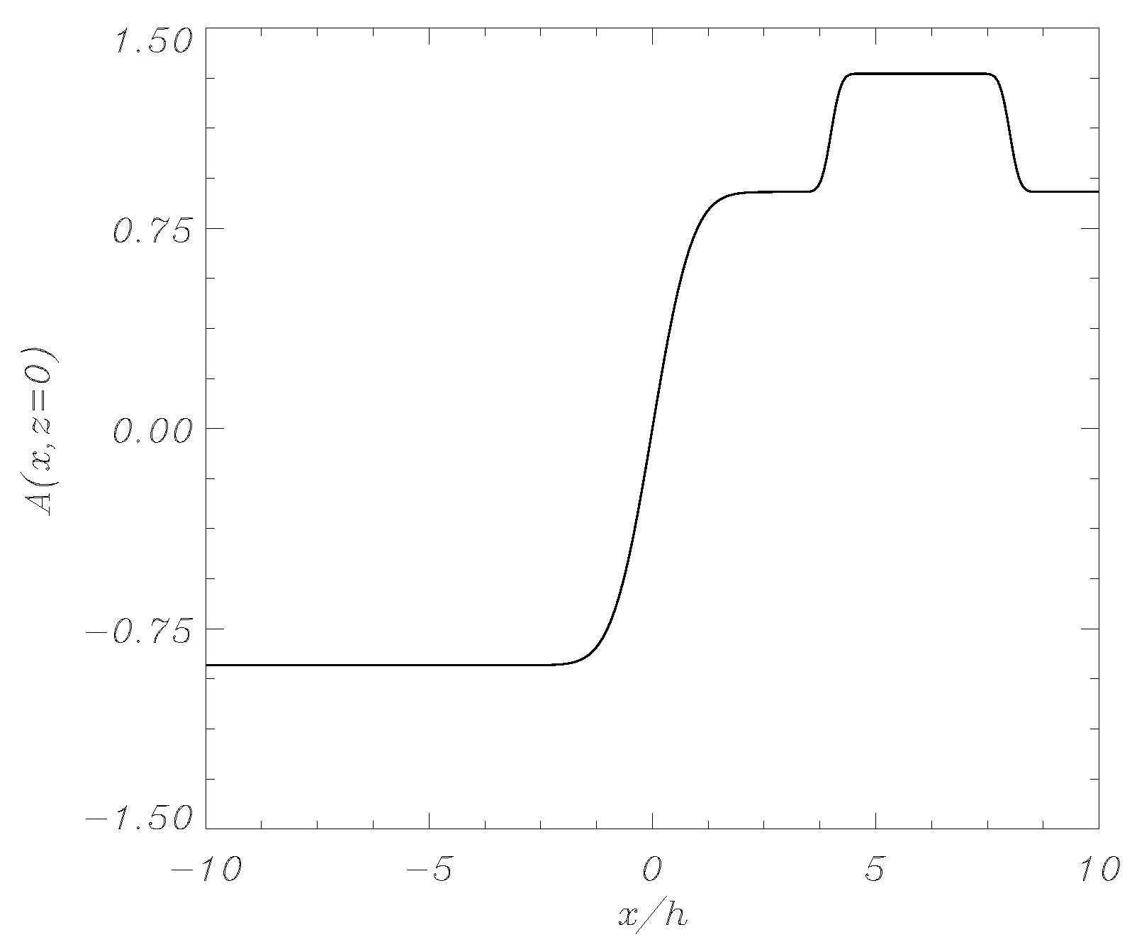
Now, let us increase the complexity of the model and consider a configuration that contains both a CH and an AR, the main aim of the present study. To this end, one just needs to use the combination of the individual CH and AR solutions given in Section 3.1 and Section 3.2 above and assume a certain separation between these two structures. A particular example is shown in Figure 1, where the CH has its center at $x=0$ and the bipolar region is located at the right of the CH (see the values of the parameters in the caption of Figure 1).

One can derive the minimum and maximum values of the flux function, which are useful for further calculations. The minimum is

$$\begin{array}{c}\hfill A_{\min }=\left(-B_0{w}_0-B_1{w}_1-B_2{w}_2\right)\frac{\sqrt{\pi }}{2},\end{array}$$

(24)

and the maximum value is

$$\begin{array}{c}\hfill A_{\max }=\left(B_0{w}_0+B_1{w}_1-B_2{w}_2\right)\frac{\sqrt{\pi }}{2}.\end{array}$$

(25)

The values (24) and (25) represent good approximations when there is no significant overlap of the tails of the Gaussian profiles of the corresponding magnetic fields. Let us note that these values are independent of the position of the bipolar region with respect to the CH, i.e., they do not depend on $x_1$ or $x_2$. To note also is that for certain values of $B_0$, $B_1$ and $w_0$ and $w_1$, $A_{\max }$ or $A_{\min }$ can also become zero and this has some important consequences for the model here considered.

Equations (24) and (25) are simplified further if a symmetric case is considered for the bipolar region, where $B_2=-B_1$ and $w_1=w_2$, such as the one plotted in Figure 1. In that case:

$$\begin{array}{c}\hfill A_{\min }=-B_0{w}_0\frac{\sqrt{\pi }}{2},\end{array}$$

(26)

which is independent of the magnetic field values at the bipolar region, while the maximum value is

$$\begin{array}{c}\hfill A_{\max }=\left(B_0{w}_0+2B_1{w}_1\right)\frac{\sqrt{\pi }}{2},\end{array}$$

(27)

which depends on the parameters of the active region.

According to Figure 1, one concludes that in the symmetric case, the value of A at the center of the CH is not altered by the presence of the bipolar region, while at the position of the AR, there is a well pronunced effect of the presence of the CH because A has increased with respect to zero due to the tail produced by the CH. In other words, in terms of the flux function A, in the symmetric situation, the CH is not affected (at its center) by the AR, but the AR is influenced by the presence of the CH.

Now, let us explore the effect of introducing a small asymmetry in the system. In order to reduce the number of parameters of the problem, let us assume that $B_2=-B_1$, but now $w_2=\alpha w_1$, where $\alpha$ is a parameter that characterizes the differences in the widths of the two unipolar magnetic regions that form the AR. Under these conditions, one finds:

$$\begin{array}{c}\hfill A_{\min }=\left(-B_0{w}_0-\{1-\alpha \}{B}_1{w}_1\right)\frac{\sqrt{\pi }}{2},\end{array}$$

(28)

and

$$\begin{array}{c}\hfill A_{\max }=\left(B_0{w}_0+\{1+\alpha \}{B}_1{w}_1\right)\frac{\sqrt{\pi }}{2}.\end{array}$$

(29)

For $\alpha =1$, the results (26) and (27) for the symmetric case are recovered, as expected.

Contrary to the symmetric case, an imbalance or asymmetry in the AR produces tails that change the value of A at the position of the CH. Therefore, the asymmetry in the bipolar region makes the CH and the AR influencing each other.

4. Coupling the Magnetic Field to the Plasma

For nonzero plasma-$\beta$, the magnetic field and the plasma are coupled. Although in the corona this parameter is small, including the gas pressure effect together with the gravity force, it provides a more complete model. The observations mostly provide information about the structure in the density (emission measure) and temperature, and these are variables that can be calculated from the models here when the gas pressure is different from zero.

4.1. Coronal Hole Thermal Structure

In the model here, a non-zero gas pressure is included in Equation (7) through the, actually, arbitrary functions $p_0\left(A\right)$ and $T(A,z)$ that need to be defined. The crucial point here is that the functional form of these variables to be constrained according to the known properties of CHs (see Ref. [1] and references therein). These functions were specifically chosen in order to have a minimum at the center of the CH and to increase smoothly with the position to match the coronal values. This creates a depletion in the pressure and temperature and therefore in the density (due to the ideal gas law) inside the CH, in agreement with the observed properties of CHs. A specific choice here is:

$$\begin{array}{c}\hfill p_0\left(A\right)=\left(p_{\mathrm{C}}-p_{\mathrm{CH}}\right){\left(\frac{A}{A_{\mathrm{ref}}}\right)}^2+p_{\mathrm{CH}},\\ \hfill T(A,z)=T\left(A\right)=\left(T_{\mathrm{C}}-T_{\mathrm{CH}}\right){\left(\frac{A}{A_{\mathrm{ref}}}\right)}^2+T_{\mathrm{CH}},\end{array}$$

(30)

where $p_{\mathrm{C}}$ and $T_{\mathrm{C}}$ are the coronal pressure and temperature values, while $p_{\mathrm{CH}}$ and $T_{\mathrm{CH}}$ are the corresponding CH values at $x=0$ because, at this position, $A(x=0,z)=0$ is imposed. There is squared dependence on the flux function, A, because, first, one needs the pressure and temperature to be positive defined (and A is not necessarily positive everywhere, see Figure 1), and second, the unipolar magnetic region should be symmetric with respect to the center of the CH because the magnetic field is symmetric (the Gaussian profile). The quadratic dependence satisfies these requirements, but this is not a unique possibility. In Equation (30), the flux function, A, is divided by a reference value, $A_{\mathrm{ref}}$, which, in the present case, is chosen to be equal to $A_{\min }$ (24); this allows us to fix the coronal values to $p_{\mathrm{C}}$ and $T_{\mathrm{C}}$ for $A=A_{\min }$. The values of $p_{\mathrm{CH}}$ and $T_{\mathrm{CH}}$ are achieved when $A=0$, i.e., when the magnetic field is vertical in the configuration used. It is assumed here that the temperature profile depends only on the magnetic field line (on A) and it has no explicit dependence on height (z), but one could choose a particular height dependence for the temperature as in Ref. [13]. Other profiles in Equation (30) can be analyzed, but the important feature is that the central values for the temperature and density must be smaller than the coronal values to properly represent the CH conditions.

Hence, based on physical grounds, one finds that the specific choice given by Equation (30) provides a plausible representation of typical CH conditions. The full 2D MHS solution is presented in Section 5 below since it requires the numerical integration of Equation (7) with the appropriate boundary conditions. For the moment, let us focus on the properties of the solutions at $z=0$.

4.2. Active Region Thermal Structure

ARs are denser and hotter than the surrounding corona. According to the dependence of the flux function on the position in a bipolar AR (with a maximum at the center of the AR), a possible choice is

$$\begin{array}{c}\hfill p_0\left(A\right)=\left(p_{\mathrm{AR}}-p_{\mathrm{C}}\right){\left(\frac{A}{A_{\mathrm{ref}}}\right)}^2+p_{\mathrm{C}},\\ \hfill T\left(A\right)=\left(T_{\mathrm{AR}}-T_{\mathrm{C}}\right){\left(\frac{A}{A_{\mathrm{ref}}}\right)}^2+T_{\mathrm{C}}.\end{array}$$

(31)

One could select a linear dependence with A instead, but if the bipolar region has a small imbalance in the parameters $B_1/w_1$ and $B_2/w_2$, then the flux function can be negative and this is not convenient to ensure positive defined pressures and temperatures. With a quadratic dependence, these issues are avoided. Using Equation (31), when $A=0$, the pressure and temperature have exact coronal values, $p_{\mathrm{C}}$ and $T_{\mathrm{C}}$. At the center of the AR, $A=A_{\mathrm{ref}}$ and therefore the pressure and temperature tend to the core values, which are $p_{\mathrm{AR}}$ and $T_{\mathrm{AR}}$. For a symmetric bipolar region, $A_{\mathrm{ref}}=A_{\max }$ and $A_{\min }=0$ (note that this is different to the situation for a CH where $A_{\mathrm{ref}}=A_{\min }$, necessary to have an underdense and cold core). Although the AR and the CH thermal structure are assumed to depend quadratically on A, there are some differences in the expressions for the pressure and temperature, in Equation (31) compared to Equation (30).

4.3. Coronal Hole Plus Active Region: Basic Model

The aim here is finding a simple model that describes at the same time a CH and a nearby AR. The point is how to define the functional dependence that provides a satisfactory picture of these two different magnetic structures. One can see that, according to Equations (30) and (31), a quadratic dependence brings a convenient description of CHs and ARs. Hence, the most straight hypothesis is to assume that the functional dependence of the pressure and temperature with the flux function is the same in the whole spatial domain that contains the two structures. This means that as a first attempt, it is logical to suppose that the form given by Equation (30) is applicable everywhere; this is a key assumption of the model here. Certainly, one has to asses whether, using this assumption, the resulting AR has properties that match the observations. As it is shown below, for some combinations of the parameters, the solutions can represent real structures, but for some other choices, one obtains unrealistic models.

Let us start by analyzing the combination of a CH solution and an AR solution in its simplest form, and concentrate on two different cases, the symmetric and the anti-symmetric situation, in relation to the properties of the bipolar region or AR.

4.3.1. Symmetric Case

This Section focuses on the values at the base of the corona and consider the case of a symmetric situation introduced before ($B_2=-B_1$, $w_1=w_2$). As soon as at $z=0$, the form of A is imposed and, therefore, the pressure and temperature profiles are given by Equation (30), one can well estimate, before solving the 2D problem numerically (this is performed in Section 5) below, the value of the variables at any point in x (at $z=0$). At the center of the AR, $A=A_{\max }$, see Figure 1, and substituting this value in the temperature profile, it leads to

$$\begin{array}{c}\hfill T_{\max }=\left(T_{\mathrm{C}}-T_{\mathrm{CH}}\right)\left(\frac{A_{\max }^2}{A_{\min }^2}\right)+T_{\mathrm{CH}}=\left(T_{\mathrm{C}}-T_{\mathrm{CH}}\right){\left(1+2\frac{B_1}{B_0}\frac{w_1}{w_0}\right)}^2+T_{\mathrm{CH}},\end{array}$$

(32)

where the expressions (26) and (27) are used for $A_{\min }$ and $A_{\max }$, respectively ($A_{\mathrm{ref}}=A_{\min }$ is kept here). Equation (32) provides a straightforward formula for the temperature at the core of the AR at $z=0$ as a function of the characteristics of the CH and the AR, namely the magnetic field intensity and the widths of the Gaussian profiles.

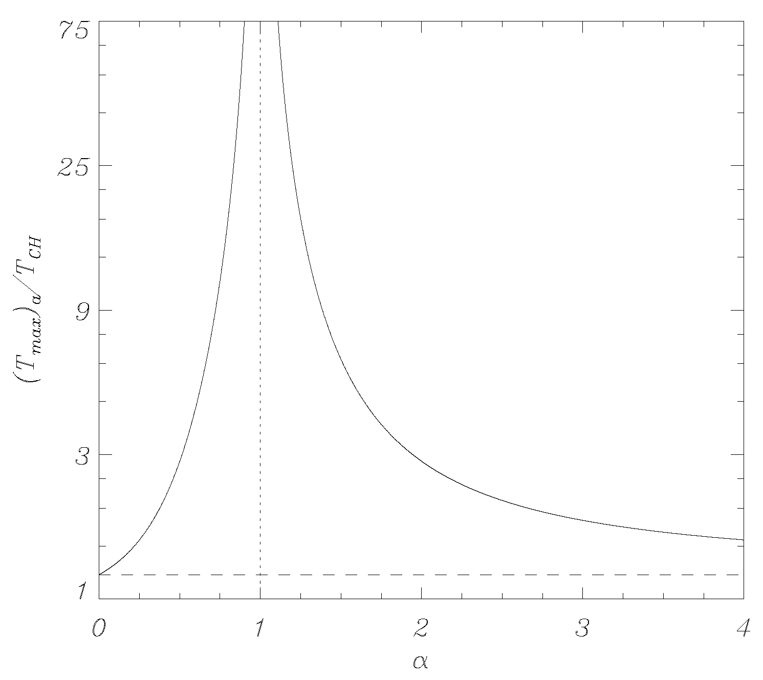
Equation (32) indicates that if $B_1/B_0$ is positive, then the maximum temperature at the center of the AR is larger than the coronal temperature (as soon as $T_{\mathrm{C}}-T_{\mathrm{CH}}>1$) i.e., the AR is hotter than the environment. This temperature enhancement of the AR grows unbounded with $B_1/B_0$ as well as with $w_1/w_0$, because these two parameters play the same role.

From Equation (32), one finds that the term inside the parentheses can be zero. This occurs when the condition

$$\begin{array}{c}\hfill B_1=-\frac{1}{2}{B}_0\frac{w_0}{w_1}\end{array}$$

(33)

is satisfied.

The latter means that when the magnetic field polarity of the AR close to the hole is the opposite to that of the hole, and with the value given by Equation (33), the core of the bipolar region is not hotter than the environment but has a CH temperature instead, because according to Equation (32), in this case, $T_{\max }=T_{\mathrm{CH}}$. Therefore, one finds the possibility of obtaining a bipolar region, with closed magnetic field lines (as shown in Section 5 below), that has CH temperatures, and this seems to be a rather unrealistic situation because there are no apparent indications in the observations if such configurations exist.

On the contrary, for $B_1$ lower than that given by Equation (33), the temperature of the AR rises again (due to the quadratic dependence of the parentheses in Equation (32)) and reaches a coronal temperature when the term inside the parentheses in Equation (32) is equal to one. This condition is achieved when

$$\begin{array}{c}\hfill B_1=-B_0\frac{w_0}{w_1}.\end{array}$$

(34)

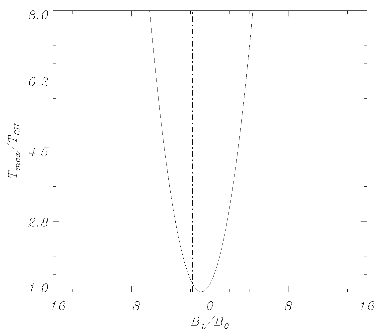
Note that, according to Equation (32), a coronal temperature is also achieved for $B_1=0$, i.e., when there is no active region. In Figure 2, $T_{\max }$ is plotted, as given by Equation (32), as a function of $B_1/B_0$ for a fixed value of $w_1/w_0$. The plot shows the features commented in this Section. Probably, the most unlikely behavior predicted by the formula in this regime is that the temperature grows unbounded as the intensity of the magnetic field increases. This issue is specifically addressed in the extended model presented later.

The possibilities found in the basic model are briefly summarized in

Table 1. Conditions that lead to realistic or unrealistic models according to the values of the magnetic field $B_0$ at the coronal hole and $B_1$ at the active region. The three regimes correspond to the three intervals that correspond to the intersection of the continuous line with the horizontal dashed line in Figure 2. $w_0$ and $w_1$ are the corresponding characteristic spatial widths.

Case 1: ${\mathit{B}}_1{\mathit{B}}_0>0$	Case 2: ${\mathit{B}}_1<-{\mathit{B}}_0{\mathit{w}}_0/{\mathit{w}}_1$	Case 3: $-{\mathit{B}}_0{\mathit{w}}_0/{\mathit{w}}_1<{\mathit{B}}_1<0$
Realistic	Realistic	Unrealistic

.

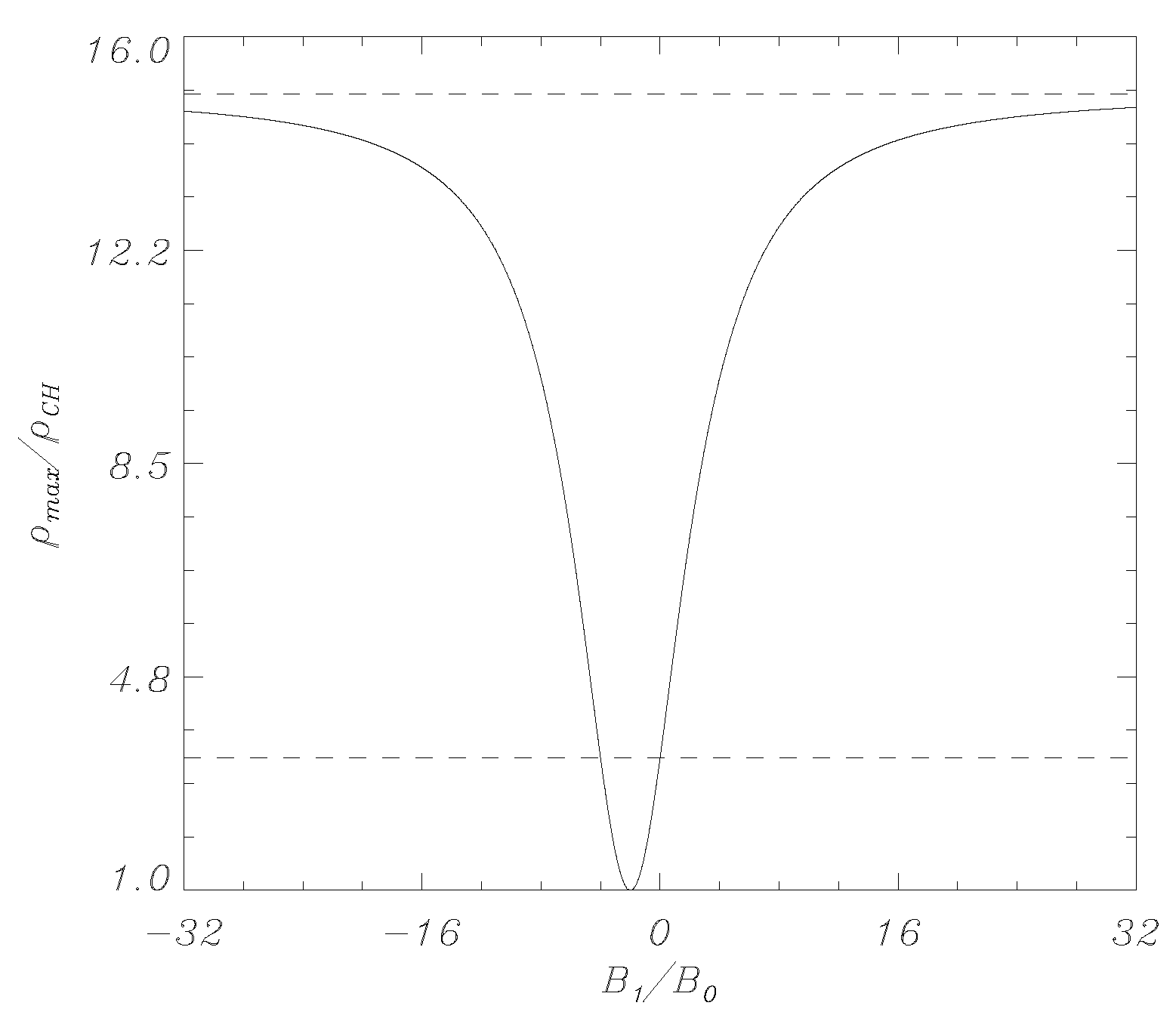
In the model considered here,, the gas pressure has exactly the same behavior as the temperature because these two magnitudes have the same dependence with A (see Equation (30)), but different functional forms could be considered. On the contrary, the plasma density in the model here is calculated from the ideal gas law and it is therefore proportional to the ratio of pressure to temperature, leading to a different dependence with the parameters. This is visualized in Figure 3, where the maximum density at the core of the AR is represented as a function of $B_1/B_0$. One obtains the following expression based on the maximum values for the temperature and pressure:

$$\begin{array}{c}\hfill {\rho }_{\max }={\rho }_{\mathrm{C}}\frac{\left(1-p_{\mathrm{CH}}/p_{\mathrm{C}}\right){\left(1+2\frac{B_1}{B_0}\frac{w_1}{w_0}\right)}^2+p_{\mathrm{CH}}/p_{\mathrm{C}}}{\left(1-T_{\mathrm{CH}}/T_{\mathrm{C}}\right){\left(1+2\frac{B_1}{B_0}\frac{w_1}{w_0}\right)}^2+T_{\mathrm{CH}}/T_{\mathrm{C}}}.\end{array}$$

(35)

One can realize that on contrary to the maximum temperature or maximum pressure, the maximum density has an upper bound, tending asymptotically to the value,

$$\begin{array}{c}\hfill {\left({\rho }_{\max }\right)}_a={\rho }_C\frac{1-p_{\mathrm{CH}}/p_{\mathrm{C}}}{1-T_{\mathrm{CH}}/T_{\mathrm{C}}},\end{array}$$

(36)

when $|B_1/B_0|$ tends to infinity. Therefore, a relevant property of this model is that the maximum density of the AR is limited to be below a certain value (that depends only on coronal and CH values), although the maximum temperature and pressure can be extremely high because they are unbounded (essentially growing as $B_1/B_0$ squared).

4.3.2. Non-Symmetric Case

In this Section, the departures from the perfectly symmetric case are investigated and it is supposed that the widths of the two unipolar magnetic fields of the AR are different, as introduced in Section 3.3 above through the parameter $\alpha$. Under these circumstances, Equations (28) and (29) are used for the minimum and maximum values of A, so that the temperature at the core of the AR, calculated as in Equation (32), yields to

$$\begin{array}{c}\hfill T_{\max }=\left(T_{\mathrm{C}}-T_{\mathrm{CH}}\right){\left[\frac{1+\left(1+\alpha \right)\frac{B_1}{B_0}\frac{w_1}{w_0}}{-1-\left(1-\alpha \right)\frac{B_1}{B_0}\frac{w_1}{w_0}}\right]}^2+T_{\mathrm{CH}}.\end{array}$$

(37)

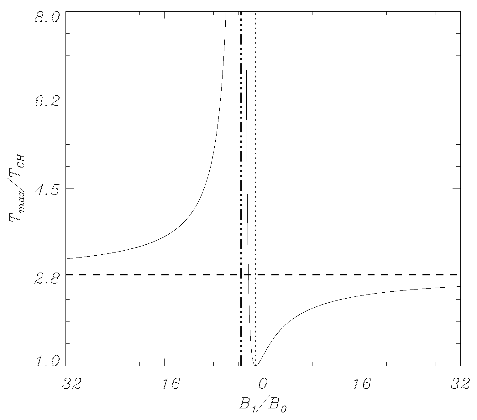
In Figure 4, the maximum AR core temperature (37) is plotted as a function of $B_1/B_0$ for the particular case, $\alpha =1/2$. The behavior of the solution is essentially different from that in the symmetric case (c.f. Figure 2).

Let us discuss the different features of the solution (37). The AR has the same temperature as the CH when

$$\begin{array}{c}\hfill B_1=-\frac{1}{1+\alpha }{B}_0\frac{w_0}{w_1},\end{array}$$

(38)

while the critical values to obtain the coronal temperature are the same as before ($B_1=-B_0{w}_0/w_1$ and $B_1=0$). Nevertheless, one finds that there is a critical value that makes $T_{\max }$ diverge. This critical value is calculated by imposing that the denominator in the first term of Equation (37) is zero (i.e., when $A_{\min }=0$), leading to

$$\begin{array}{c}\hfill B_1=-\frac{1}{1-\alpha }{B}_0\frac{w_0}{w_1}.\end{array}$$

(39)

For magnetic fields close to the value (39), the temperature of the AR tends to infinity, which is nonphysical. This corresponds to the case with $A_{\min }=0$, and being the denominator in Equation (37), the temperature (and pressure) grows unbounded. The extended model presented in Section 4.4 below does not demonstrate such a behavior.

However, an interesting feature is that for $B_1/B_0>0$, the temperature is now bounded and tends asymptotically from below (see the thick horizontal dashed line in Figure 4) to the value

$$\begin{array}{c}\hfill {\left(T_{\max }\right)}_a=\left(T_{\mathrm{C}}-T_{\mathrm{CH}}\right){\left(\frac{1+\alpha }{1-\alpha }\right)}^2+T_{\mathrm{CH}},\end{array}$$

(40)

while in the symmetric case, one finds an unbounded increasing temperature. The same asymptote is found for the case $B_1/B_0<0$. In Figure 5, the asymptotic temperature Equation (40) is shown as a function of $\alpha$. Only in the symmetric case ($\alpha =1$) the behavior is singular. In this respect, the non-symmetric case provides a more realistic behavior than the symmetric one as soon as the former is non-divergent for a wider range of values of $B_1/B_0$. In reality, the ideally symmetric case does not exist, and, therefore, the magnetic field configurations are more similar to the non-symmetric cases discussed here.

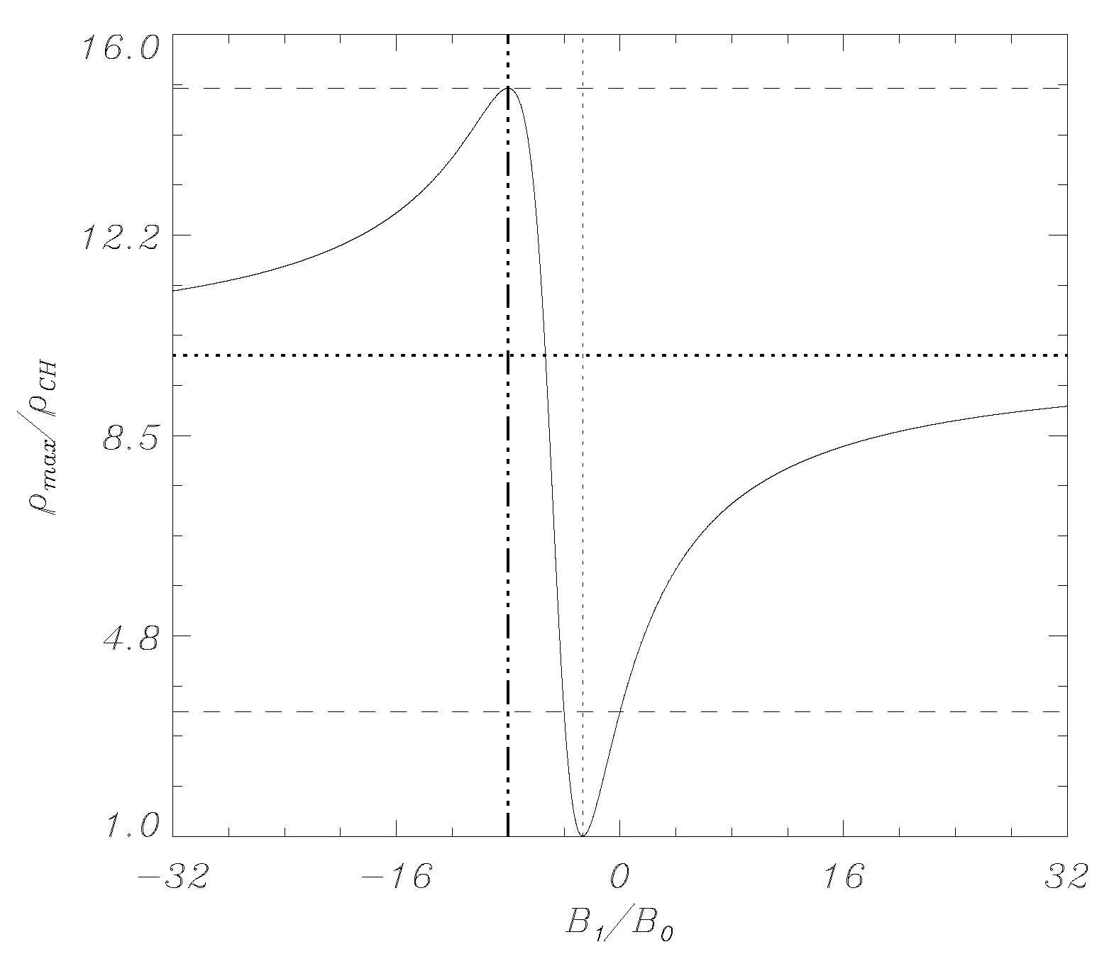
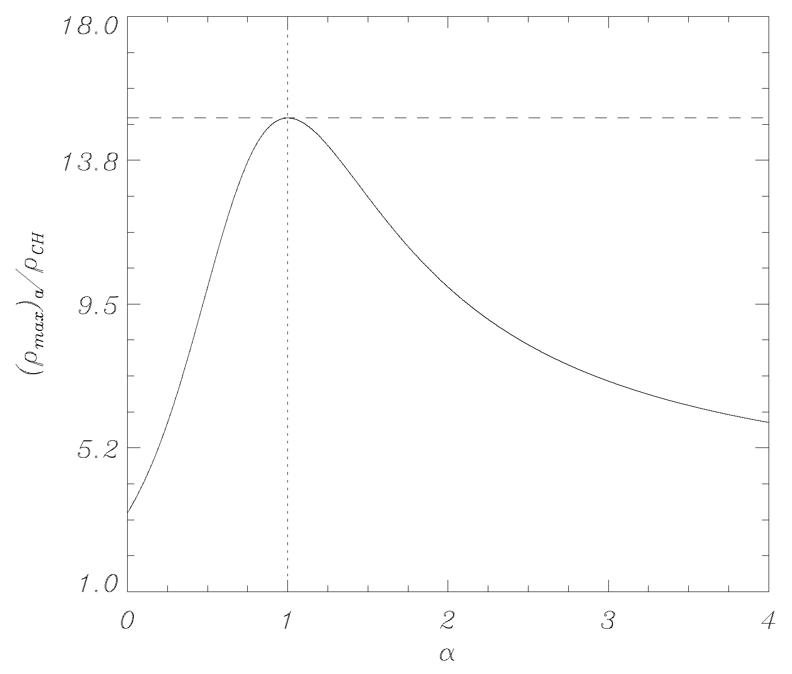
The maximum density is calculated as in Section 4.3.1, and is plotted in Figure 6. This variable is now bounded and has a maximum value that is exactly the asymptotic value (36) obtained for the symmetric case and is located precisely at the position where the temperature and pressure are unbounded. The maximum density shows a new asymptote for $|B_1/B_0|$ being large enough. This asymptotic value is

$$\begin{array}{c}\hfill {\left({\rho }_{\max }\right)}_a={\rho }_{\mathrm{C}}\frac{\left(1-p_{\mathrm{CH}}/p_{\mathrm{C}}\right){\left(\frac{1+\alpha }{1-\alpha }\right)}^2+p_{\mathrm{CH}}/p_{\mathrm{C}}}{\left(1-T_{\mathrm{CH}}/T_{\mathrm{C}}\right){\left(\frac{1+\alpha }{1-\alpha }\right)}^2+T_{\mathrm{CH}}/T_{\mathrm{C}}}.\end{array}$$

(41)

The asymptotic maximum density (41) is plotted in Figure 7 as a function of $\alpha$. The maximum density value is obtained for the symmetric case ($\alpha =1$), which means that the asymmetry in the widths of the bipolar regions always tends to reduce the asymptotic maximum density at the core of the AR.

4.4. Extended Model

The basic model described in Section 4.3 shows some features that look unrealistic. For this reason, let us construct another model that specifically addresses at least part of the limitations of the basic model. In particular, let us propose alternative pressure and temperature profiles that enforce these magnitudes to be bounded for large enough $|B_1/B_0|$, the main shortcoming of the basic model. Let us use the following alternative definitions:

$$\begin{array}{c}\hfill p_0\left(A\right)=\left(p_{\mathrm{CB}}-p_{\mathrm{CH}}\right){tanh}^2\left(a\frac{A}{A_{\mathrm{ref}}}\right)+p_{\mathrm{CH}},\end{array}$$

(42)

$$\begin{array}{c}\hfill T\left(A\right)=\left(T_{\mathrm{CB}}-T_{\mathrm{CH}}\right){tanh}^2\left(a\frac{A}{A_{\mathrm{ref}}}\right)+T_{\mathrm{CH}},\end{array}$$

(43)

where $p_{\mathrm{CB}}$ and $T_{\mathrm{CB}}$ are the maximum values (bounds) for coronal pressure and temperature. Defining again the coronal reference at $A=A_{\mathrm{ref}}$, from the temperature profile (43), one has:

$$\begin{array}{c}\hfill T_{\mathrm{C}}=\left(T_{\mathrm{CB}}-T_{\mathrm{CH}}\right){tanh}^{2}a+T_{\mathrm{CH}},\end{array}$$

(44)

which has been rewritten as

$$\begin{array}{c}\hfill T_{\mathrm{CB}}-T_{\mathrm{CH}}=\frac{T_{\mathrm{C}}-T_{\mathrm{CH}}}{{tanh}^{2}a},\end{array}$$

(45)

corresponds to the multiplicative factor in the first term of Equation (43). Then, the parameter a is

$$\begin{array}{c}\hfill a=\mathrm{atanh}\left(\sqrt{\frac{T_{\mathrm{C}}-T_{\mathrm{CH}}}{T_{\mathrm{CB}}-T_{\mathrm{CH}}}}\right),\end{array}$$

(46)

at the given CH temperature, coronal reference temperature, and maximum coronal temperature. Note that a is not a small dimensionless number.

The maximum value for the coronal gas pressure, once a is known, is calculated from

$$\begin{array}{c}\hfill p_{\mathrm{CB}}=\frac{p_{\mathrm{C}}-p_{\mathrm{CH}}}{{tanh}^{2}a}+p_{\mathrm{CH}},\end{array}$$

(47)

which is equivalent to Equation (45) for the temperature.

4.4.1. Symmetric Case

Now, in this model, based on Equations (42) and (43), the maximum values of the temperature and pressure are bounded for quite large $|B_1/B_0|$ and tending by construction to $T_{\mathrm{CB}}$ and $p_{\mathrm{CB}}$, respectively. The explicit expression for the maximum temperature is

$$\begin{array}{c}\hfill T_{\max }=\frac{T_{\mathrm{C}}-T_{\mathrm{CH}}}{{tanh}^{2}a}{tanh}^2\left[-a\left(1+2\frac{B_1}{B_0}\frac{w_1}{w_0}\right)\right]+T_{\mathrm{CH}}.\end{array}$$

(48)

If $T_{\mathrm{CB}}\gg T_{\mathrm{C}}$, then $a\ll 1$, and using the MacLaurin expansion for tanh and keeping the first term of the series ($tanhx\approx x$), one obtains the same expression as for the basic model, see Equation (32). However, a is not necessarily a small parameter. Note that Equation (48) has a maximum value of $T_{\mathrm{CB}}$ for large enough $|B_1/B_0|$, but in case the term in the brackets is zero, $T_{\max }=T_{\mathrm{CH}}$. This is exactly the same behavior that was found for the basic model in Section 4.3.1 above. Therefore, the extended model keeps the maximum temperature value bounded but allows the possibility of obtaining a cool AR core for a certain combination of the parameters, see Equation (33).

It is straightforward to see that the maximum density of the AR is given by

$$\begin{array}{c}\hfill {\left({\rho }_{\max }\right)}_a={\rho }_C\frac{1-p_{\mathrm{CH}}/p_{\mathrm{C}}\left(1-{tanh}^{2}a\right)}{1-T_{\mathrm{CH}}/T_{\mathrm{C}}\left(1-{tanh}^{2}a\right)}.\end{array}$$

(49)

In the limit $a\ll 1$, one obtains the same expression as for the basic model, see Equation (36).

4.4.2. Non-Symmetric Case

For the extended model, the maximum temperature at the core of the AR in the non-symmetric case is

$$\begin{array}{c}\hfill T_{\max }=\frac{T_{\mathrm{C}}-T_{\mathrm{CH}}}{{tanh}^{2}a}{tanh}^2\left[a\frac{1+\left(1+\alpha \right)\frac{B_1}{B_0}\frac{w_1}{w_0}}{-1-\left(1-\alpha \right)\frac{B_1}{B_0}\frac{w_1}{w_0}}\right]+T_{\mathrm{CH}}.\end{array}$$

(50)

Then, in the limit of large enough $|B_1/B_0|$, the asymptotic value is

$$\begin{array}{c}\hfill {\left(T_{\max }\right)}_a=\frac{T_{\mathrm{C}}-T_{\mathrm{CH}}}{{tanh}^{2}a}{tanh}^2\left(a\frac{1+\alpha }{-1+\alpha }\right)+T_{\mathrm{CH}}.\end{array}$$

(51)

Using again the expansion for small arguments of tanh (if a is small, the argument of tanh is also small, except when $\alpha$ tends to one), one finds that Equation (51) reduces to Equation (40) for the basic model. Again, the two models have the same asymptotic values for the temperature and pressure.

The asymptotic maximum density is

$$\begin{array}{c}\hfill {\left({\rho }_{\max }\right)}_a={\rho }_C\frac{\left(1-p_{\mathrm{CH}}/p_{\mathrm{C}}\right){tanh}^2\left(a\frac{1+\alpha }{-1+\alpha }\right)+p_{\mathrm{CH}}/p_{\mathrm{C}}{tanh}^{2}a}{\left(1-T_{\mathrm{CH}}/T_{\mathrm{C}}\right){tanh}^2\left(a\frac{1+\alpha }{-1+\alpha }\right)+T_{\mathrm{CH}}/T_{\mathrm{C}}{tanh}^{2}a}.\end{array}$$

(52)

For small a, Equation (52) tends to the expression obtained for the basic model, Equation (41).

Hence, it is shown that it is possible to construct an improved model with respect to the basic model with a maximum temperature and pressure that do not have an unlimited growth with $|B_1/B_0|$. This model is more realistic from the physical point of view, but it still allows to have closed magnetic field lines with CH temperatures, the latter is rather improbable.

5. Numerical Results

The analytical approach considered in Section 3 and Section 4 is based on the values of the flux function, pressure and temperature at the lower boundary ($z=0$). However, one still needs to find the full solution in the plane x-z. It is crucial to understand how the topology of the magnetic field changes according to the values of the parameters and how the connection between the CH and the nearby bipolar region is established. In general, finding solutions to Equation (7) requires numerical methods unless the profile for $p\left(A\right)$ and the boundary conditions are quite simple. Only in the case that Equation (7) is a linear equation, general analytical methods are available. However, this is quite a complicated task at this point, and for this reason, Equation (7) was solved numerically. For the details about the numerical method used, see [13]. Here, it is sufficient to mention that the numerical code PDE2D [22] was used which solves, via the method of finite elements, partial differential equations of the type found in the problem under consideration.

The numerical solutions for individual CHs and ARs were described in detail in Ref. [13] and will be not repeated here. Let us focus on the most simple case of a configuration that combines these two structures and investigate the characteristics of the solutions in 2D. For simplicity reasons, a focus is on the symmetric case introduced earlier in Section 4.3.1, and not on the results for the non-symmetric case discussed in Section 4.3.2. Moreover, the analysis here is restricted to the basic model, although equivalent results were found for the extended model. It is convenient to remind that when the parameter a is small, the extended model reduces to the basic model. There is also a technical reason as well to focus on the basic model; the convergence of the numerical method for the extended model is much slower than that for the basic model.

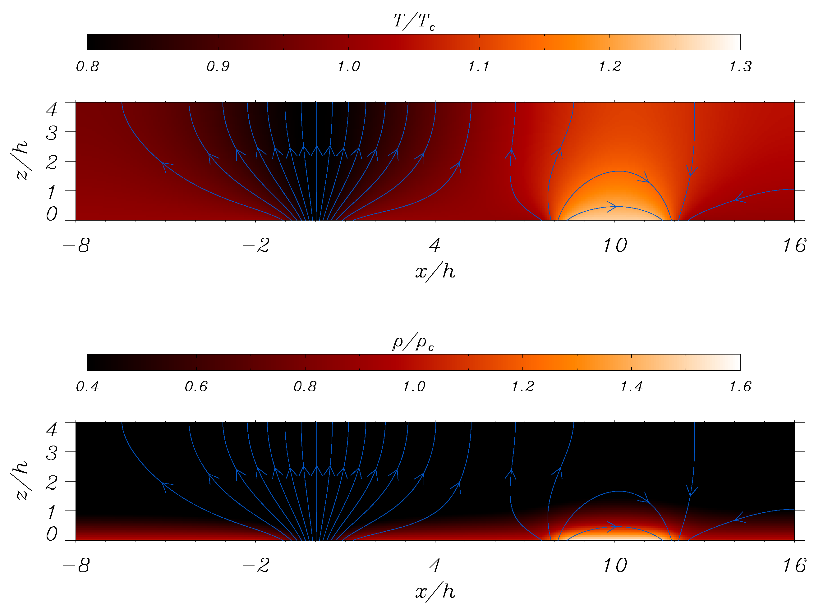
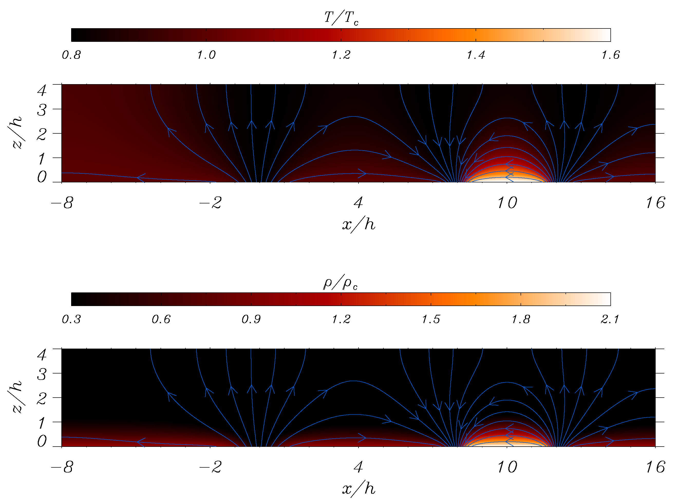
Figure 8 shows a numerical solution that contains both a CH (located at $x=0$) and an AR located on the right part of the spatial domain ($x_1/h=8$ and $x_2/h=12$). In this example, the left foot of the AR has the same polarity as the CH ($B_0{B}_1>0$) (case 1 in Table 1). The temperature and density are low inside the CH, while these magnitudes are high in the AR in comparison with the coronal environment. Using the same functional form for the functions $p\left(A\right)$ and $T\left(A\right)$, one obtains a rather smooth solution in the x-z plane. The maximum temperature and density values at the core of the AR agree with the derived analytical values given by Equations (32) and (35). For the present choice of parameters, this is the case pointing to the right of the reference value located at $B_1/B_0=0$ in Figure 2 and Figure 3.

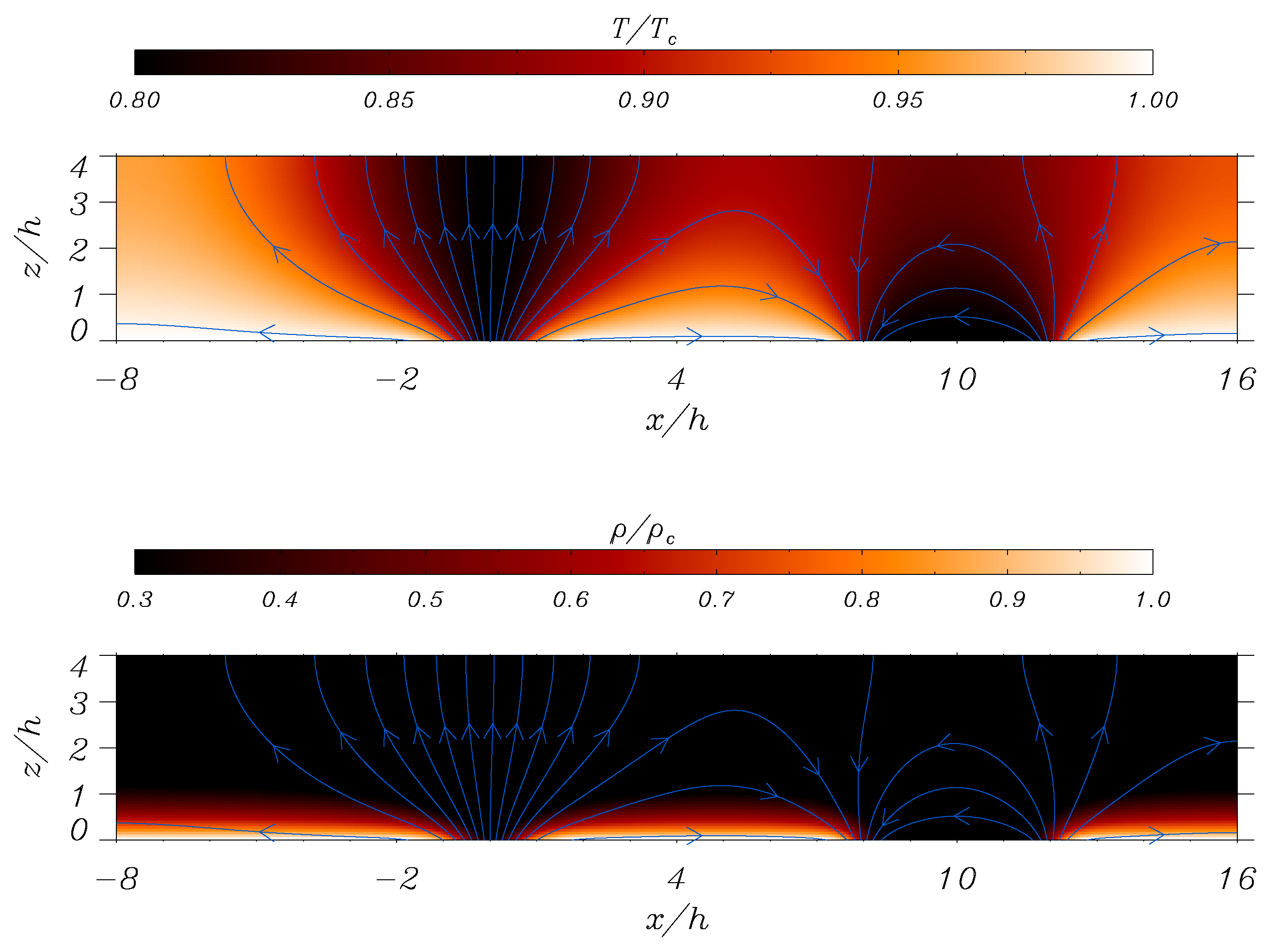
Figure 9 is similar to Figure 8, but the left foot of the AR has the opposite polarity to that of the CH ($B_0{B}_1<0$). It corresponds to a point to the left of the value $|B_1/B_0|<w_0/w_1$ in Figure 2 and Figure 3 (case 2 in Table 1). Again, the temperature and density are low inside the CH, but the differences arise essentially in the AR and near the corresponding footpoints. The temperature and density are high inside the AR, but next to the two footpoints (located at $x_1/h=8$ and $x_2/h=12$), one finds a depletion in the temperature and density that remind of the behavior inside the CH. This is not surprising as soon as one realizes that the magnetic field lines are essentially open and expanding with a height around $x_1$ and $x_2$ in a way similar to that in the CH located at $x=0$. Another relevant feature of the MHS solution of the present example is that the temperature above the AR ($z\ge 2h$) does not tend to the coronal temperature as in Figure 8 and it is closer to the CH temperature instead; therefore, the AR is essentially surrounded and embedded by a cool and low-density plasma.

The last example of the type of solutions allowed in the model here is shown in Figure 10. The configuration is specifically chosen to have a magnetic field in the AR that is between the values given by Equations (33) and (34) (Case 3 in Table 1), i.e., the difference with respect to the results shown in Figure 8 and Figure 9 is just the value of the magnetic field at the AR. For this case, one obtains a CH with basically the same properties as in Figure 8 and Figure 9, but the peculiarity relies on the bipole. The AR in this model is characterized by a low temperature and a low density in comparison with the coronal environment. Therefore, the closeness of the magnetic field lines does not necessarily indicate that the bipolar region must have a hot and dense core according to the solutions found. In this region, a void in the density and temperature is possible according to the model here. This configuration is the most peculiar, and most likely unrealistic, of the three examples shown in Figure 8, Figure 9 and Figure 10.

6. Conclusions and Discussion

In this paper, MHS models that represent a compound of a CH and an AR are constructed using the formalism of Ref [13]. 2D magnetostatic equilibria were generated by solving the Grad–Shafranov equation. The magnetic field arrangement, chosen to represent both open and closed magnetic field lines, is incorporated through the boundary conditions needed to solve the partial differential equation. A relatively simple functional form was used for the plasma pressure and temperature in terms of the flux function. The use of a common functional dependence for the thermal structure allows us to study the properties of an MHS equilibrium that contains a CH, taken as the reference structure, and an AR situated at a certain distance from the CH. This is the key assumption in this paper. Interestingly, the same functional form describes correctly the general features of both CHs (low pressure, temperature and density) and ARs (high pressure, temperature and density) at least in two of the three types of the models presented in this paper. The exact form of the pressure and temperature functions considered in the present study is not relevant. Other choices can also lead to physically acceptable solutions. The contribution of the model considered relies on the finding of solutions that can represent concurrently two different magnetic structures with properties similar to those reported by the observations. It is worth mentioning that the construction of models with different spatial dependencies according to the spatial location in the domain is still possible but much more complex than the situation explored in the present case. Hence, a different functional form for the CH and the AR could be considered. This needs to be addressed in future studies because it can lead to models that do not show unphysical or unobserved configurations like the ones reported here.

The study analyzed how the main parameters of one structure depend on the parameters of the other. In this regard, the novelty of the solutions obtained in the present paper is that they provide information about the coupling between the two structures, an effect that was not yet addressed in the literature, as to the author’s knowledge. This interplay between the two configurations is due to a) the common functional form assumed for the pressure and temperature and b) the topology of the magnetic field, i.e., how the global magnetic structure combines the joint effect of the presence of the CH and AR.

When the bipolar magnetic configuration is perfectly symmetric, i.e., has a net zero magnetic flux, keeping the parameters of the CH constant and using as a reference the mean coronal values for the temperature and pressure, three essentially different types of bipolar solutions or ARs are found. These solutions basically depend on the magnitude and especially on the sign of the magnetic field at the footpoints, $B_1$, see also Table 1:

• When the closest foot of the bipolar configuration to the CH and the CH itself have the same magnetic polarity, a solution resembling a typical AR with closed field lines embedding a hot and dense core is obtained.
• When the magnetic field of the bipolar foot is below $-B_0{w}_0/w_1$ and therefore the CH and the closest AR foot have an opposite polarity, one again obtains a case of an AR with a hot and dense core. However, the magnetic field lines near the footpoints of the AR are essentially open and the plasma has low values of the pressure, temperature and density there. The AR is surrounded by cold and light plasma, instead. Hence, the configuration may resemble that of multiple CHs located near the AR or even a dark halo.
• When the polarity of the CH and the closest foot of the bipolar region are opposite, but the magnetic field of the foot and $B_1$ is in the range from 0 to $-B_0{w}_0/w_1$, one finds closed magnetic field lines filled with plasma with the pressure, temperature and density below the coronal reference values and reaching a minimum at CH values. The plasma conditions are therefore that of typical CHs but with closed magnetic field lines in nearby locations.

The results presented in this paper shed light on the possible relationship between CHs and nearby ARs and provide new information that should be carefully contrasted with observations. The models considered here predict the existence of three different types of bipolar regions interacting with CHs. It is apparent that the first type of solution, i.e., the standard AR configuration, is observed routinely. This is the most common case. The second type of configuration could be related to the existence of several CHs reported on the disk, and under some conditions, it could be related to the presence of outflows at the edge of the ARs (see [5]) just because the magnetic field can be locally open there, as shown in the solutions found here. Actually, there are observations where the CH presumably extends to the edge of an AR or even surrounds it, but since the emission of the AR is too strong compared to the CH, these dark regions are difficult to be observed. The third type of solution is the most difficult to interpret because in general the observations do not show dark ARs. Nevertheless, there are cases where an AR disappears and a CH appears afterward precisely at the same location.

In such a configuration, the third type of solution could be possible but for a highly limited time before the AR transforms into a pure CH. Long observations are required to understand this case because the appearance of a CH at the same location of an AR is a process that takes several days/weeks, longer than the usual observing periods.

Simple analytical expressions are obtained here for the pressure, temperature and density at the core of the AR and their dependence were studied upon several major physical parameters, such as the intensity of the magnetic field and the width of the magnetic spatial distribution at the reference level $z=0$. Two different models were investigated, the substantial difference among them being that in the extended model the temperature and pressure do not grow unbounded with the magnetic field of the AR, while in the basic model they do. In the extended model, it was imposed that the temperature and pressure can not be larger than a certain value and this leads to the redefinition of the dependence of the temperature and pressure on the flux function.

The situation for an AR with a certain imbalance in the magnetic flux was also considered, and this corresponds to the asymmetric case. This is a more realistic setting according to photospheric magnetograms. An interesting result under such asymmetry conditions is that the relevant magnitudes tend to asymptotic values when $|B_1/B_0|$ is significantly high. In this limit, the two models proposed here have restrained maximum pressure, temperature and density values at the core of the AR, and the exact magnetic field value of the AR in this situation is indeed not of much importance. Hence, an additional constrain anticipated by the model here is the existence of a maximum density at the core of the AR. This quantity is essentially independent of the magnetic field of the AR as long as $B_1$ is much larger than that at the center of the CH, $B_0$. This maximum critical density depends only on the coronal reference values and on the plasma pressure and temperature at the center of the CH.

The family of solutions calculated numerically can be used, among other findings to study the process of the emergence of a magnetic flux adjacent to a CH. The emergence can involve a wide variety of time scales, but under some circumstances, the premise can be used that the magnetic field, which is coupled to the plasma in the model here considered, evolves through a series of equilibrium states (see, e.g., [23,24]). These equilibrium states are precisely the MHS solutions that were obtained from the calculations. This method, that can be considered complementary to the full MHD modeling, provides useful information about the topology of the magnetic field without the requirement of an accurate physical description of the reconnection process that needs to be implemented, often using various approximations, in the time-dependent MHD simulations. By smoothly increasing the magnetic field of the bipolar region ($B_1$) from zero and up to a certain value, the connectivity of the system has to change, and some field lines that were open become closed, and vice versa. In particular, open lines belonging to the right part of the CH become closed while initially closed lines rooted on the right edge of the bipolar region may transform into open. This is the essence of the process of an interchange reconnection (see [7,25,26]). Interestingly, there is observational evidence of an emerging magnetic flux interacting with CHs supporting this mechanism ([27,28,29]), and the theoretical models studied in the present paper can be useful.

It is imperative to mention that in the models proposed in this paper, several important processes that can have a relevant effect on the results were ignored. No presence of flows, ubiquitous in CHs as well as in ARs were considered. From the theoretical point of view, the inclusion of flows can be performed using the approaches of Refs. [2,3] (see also [30]). In this case, the Grad–Shafranov equation is coupled to the Bernoulli equation. Nevertheless, fast flows of the order of the Alfvén velocity, which are typically below the observed ones (see [1]), are needed to produce significant changes in the MHS equilibrium.

Another critical point of the approach used in this study is that the energy equation is not treated self-consistently. Among other difficulties, the exact form of the heating function in the corona is still unknown. For this reason, Ref. [13] have tried to determine this heating function based on the constrains of the force balance and thermal balance. These authors find regions where the energy balance is not possible, and this depends on the scale of the temperature variation with a height that eventually modifies the conduction and the radiative losses in the system. In the present paper, it was preferred not to address this problem, while leaving it for future studies, and focussed on the force balance only. Including self-consistency and an energy equation can be performed using the approach of Ref. [31].

The 2D models studied here might seem be too idealized to represent a real 3D structure, such as a CH or an AR. The 2D models are applicable when the structure is invariant in one direction (the y-direction in this case). The use of the flux function allows us to simplify the problem. In 3D, the equilibrium of the forces require more complicated calculations and a numerical treatment is unavoidable. For example, using two Euler potentials, the equivalent counterparts of the flux function in 2D, one obtains two equations that provide the force balance across the magnetic field (see, e.g., [32,33]). This was recently investigated in Ref. [34], where open and closed magnetic field lines in 3D are able to coexist under the presence of gravity. The procedure in Ref. [34] can be used to investigate the features of the combination of a CH and an AR in 3D in an equivalent form, as was performed in 2D in the present paper.

Concluding, let us stress that an elementary understanding of the interplay between CHs and ARs using MHS models is essential before additional effects are added to the problem.

References

- Cranmer, S.R. Coronal holes. Living Rev. Sol. Phys. 2009, 6, 3. [Google Scholar] [CrossRef] [Green Version]
- Tsinganos, K.C. Magnetohydrodynamic equilibrium. I. Exact solutions of the equations. Astrophys. J. 1981, 245, 764–782. [Google Scholar] [CrossRef]
- Tsinganos, K.C. Magnetohydrodynamic equilibrium. II. General integrals of the equations with one ignorable coordinate. Astrophys. J. 1982, 252, 775–790. [Google Scholar] [CrossRef]
- Low, B.C.; Tsinganos, K. Steady hydromagnetic flows in open magnetic fields. I. A class of analytic solutions. Astrophys. J. 1986, 302, 163–187. [Google Scholar] [CrossRef]
- van Driel-Gesztelyi, L.; Culhane, J.L.; Baker, D.; Démoulin, P.; Mandrini, C.H.; DeRosa, M.L.; Rouillard, A.P.; Opitz, A.; Stenborg, G.; Vourlidas, A.; et al. Magnetic topology of active regions and coronal holes: Implications for coronal outflows and the solar wind. Sol. Phys. 2012, 281, 237–262. [Google Scholar] [CrossRef] [Green Version]
- Harra, L.K.; Sakao, T.; Mandrini, C.H.; Hara, H.; Imada, S.; Young, P.R.; van Driel-Gesztelyi, L.; Baker, D. Outflows at the edges of active regions: Contribution to solar wind formation? Astrophys. J. 2008, 676, L147–L150. [Google Scholar] [CrossRef] [Green Version]
- Masson, S.; Antiochos, S.K.; DeVore, C.R. Escape of flare-accelerated particles in Solar eruptive events. Astrophys. J. 2019, 884, 143. [Google Scholar] [CrossRef] [Green Version]
- Piantschitsch, I.; Vršnak, B.; Hanslmeier, A.; Lemmerer, B.; Veronig, A.; Hernandez-Perez, A.; Čalogović, J. Numerical simulation of coronal waves interacting with coronal holes. II. Dependence on Alfvén speed inside the coronal hole. Astrophys. J. 2018, 857, 130. [Google Scholar] [CrossRef]
- Piantschitsch, I.; Vršnak, B.; Hanslmeier, A.; Lemmerer, B.; Veronig, A.; Hernandez-Perez, A.; Čalogović, J. Numerical simulation of coronal waves interacting with coronal holes. III. Dependence on initial amplitude of the incoming wave. Astrophys. J. 2018, 860, 24. [Google Scholar] [CrossRef]
- Piantschitsch, I.; Terradas, J.; Temmer, M. A new method for estimating global coronal wave properties based on their interaction with solar coronal holes. Astron. Astrophys. 2020, 641, A21. [Google Scholar] [CrossRef]
- Piantschitsch, I.; Terradas, J. Geometrical properties of the interaction between oblique incoming coronal waves and coronal holes. Astron. Astrophys. 2021, 651, A67. [Google Scholar] [CrossRef]
- Downs, C.; Roussev, I.I.; van der Holst, B.; Lugaz, N.; Sokolov, I.V.; Gombosi, T.I. Studying extreme ultraviolet wave transients with a digital laboratory: Direct comparison of extreme ultraviolet wave observations to global magnetohydrodynamic simulations. Astrophys. J. 2011, 728, 2. [Google Scholar] [CrossRef] [Green Version]
- Terradas, J.; Soler, R.; Oliver, R.; Antolin, P.; Arregui, I.; Luna, M.; Piantschitsch, I.; Soubrié, E.; Ballester, J.L. Construction of coronal hole and active region magnetohydrostatic solutions in two dimensions: Force and energy balance. Astron. Astrophys. 2022, 660, A136. [Google Scholar] [CrossRef]
- Aschwanden, M.J.; Newmark, J.S.; Delaboudinière, J.P.; Neupert, W.M.; Klimchuk, J.A.; Gary, G.A.; Portier-Fozzani, F.; Zucker, A. Three-dimensional stereoscopic analysis of solar active region loops. I. SOHO/EIT observations at temperatures of (1.0–1.5) × 106 K. Astrophys. J. 1999, 515, 842–867. [Google Scholar] [CrossRef] [Green Version]
- Aschwanden, M.J.; Alexander, D.; Hurlburt, N.; Newmark, J.S.; Neupert, W.M.; Klimchuk, J.A.; Gary, G.A. Three-dimensional stereoscopic analysis of solar active region loops. II. SOHO/EIT observations at temperatures of 1.5–2.5 MK. Astrophys. J. 2000, 531, 1129–1149. [Google Scholar] [CrossRef]
- Low, B.C. Nonisothermal magnetostatic equlibria in a uniform gravity field. I. Mathematical formulation. Astrophys. J. 1975, 197, 251–255. [Google Scholar] [CrossRef]
- Parker, E.N. The dynamical state of the interstellar gas and field. V. Reduced dynamical equations. Astrophys. J. 1968, 154, 57–72. [Google Scholar] [CrossRef]
- Parker, E.N. Cosmical Magnetic Fields: Their Origin and Their Activity; Clarendon Press (Oxford University Press): New York, NY, USA, 1979. [Google Scholar]
- Priest, E.R. Solar Magnetohydrodynamics; Reidel Publishing Company: Dordrecht, The Netherlands, 1982. [Google Scholar] [CrossRef]
- Priest, E.; Forbes, T. Magnetic Reconnection. MHD Theory and Applications; Cambridge University Press: Cambridge, UK, 2009. [Google Scholar] [CrossRef]
- Pizzo, V.J. Numerical solution of the magnetostatic equations for thick flux tubes, with application to sunspots, pores, and related structures. Astrophys. J. 1986, 302, 785–808. [Google Scholar] [CrossRef]
- Sewell, G. The Numerical Solution of Ordinary and Partial Differential Equations; John Wiley & Sons, Inc.: Hoboken, NJ, USA, 2005. [Google Scholar] [CrossRef]
- Priest, E.R.; Milne, A.M. Force-free magnetic arcades relevant to two-ribbon solar flares. Sol. Phys. 1980, 65, 315–346. [Google Scholar] [CrossRef]
- Forbes, T.G. Magnetic reconnection in solar flares. Geophys. Astrophys. Fluid Dyn. 1991, 62, 15–36. [Google Scholar] [CrossRef]
- Gosling, J.T.; Birn, J.; Hesse, M. Three-dimensional magnetic reconnection and the magnetic topology of coronal mass ejection events. Geophys. Res. Lett. 1995, 22, 869–872. [Google Scholar] [CrossRef]
- Crooker, N.U.; Gosling, J.T.; Kahler, S.W. Reducing heliospheric magnetic flux from coronal mass ejections without disconnection. J. Geophys. Res. Space Phys. 2002, 107, 1028. [Google Scholar] [CrossRef] [Green Version]
- Baker, D.; van Driel-Gesztelyi, L.; Attrill, G.D.R. Evidence for interchange reconnection between a coronal hole and an adjacent emerging flux region. Astron. Not./Astron. Nachr. 2007, 328, 773–776. [Google Scholar] [CrossRef]
- Ma, L.; Qu, Z.Q.; Yan, X.L.; Xue, Z.K. Interchange reconnection between an active region and a coronal hole. Res. Astron. Astrophys. 2014, 14, 221–228. [Google Scholar] [CrossRef] [Green Version]
- Kong, D.F.; Pan, G.M.; Yan, X.L.; Wang, J.C.; Li, Q.L. Observational evidence of interchange reconnection between a solar coronal hole and a small emerging active region. Astrophys. J. Lett. 2018, 863, L22. [Google Scholar] [CrossRef]
- Schindler, K. Physics of Space Plasma Activity; Cambridge University Press: New York, NY, USA, 2007. [Google Scholar] [CrossRef] [Green Version]
- Low, B.C.; Berger, T.; Casini, R.; Liu, W. The hydromagnetic interior of a solar quiescent prominence. I. Coupling between force balance and steady energy transport. Astrophys. J. 2012, 755, 34. [Google Scholar] [CrossRef] [Green Version]
- Stern, D. Geomagnetic Euler potentials. J. Geophys. Res. 1967, 72, 3995–4005. [Google Scholar] [CrossRef] [Green Version]
- Stern, D.P. Euler potentials. Am. J. Phys. 1970, 38, 494–501. [Google Scholar] [CrossRef]
- Terradas, J.; Neukirch, T. Three-dimensional solar active region magnetohydrostatic models and their stability using Euler potentials. arXiv 2022, arXiv:2212.04735. [Google Scholar] [CrossRef]
Figure 1.
Flux function as a function of the horizontal position at for the combination of a coronal hole (CH) and a bipolar region. Here, , , , , , and . See text for details.
Figure 2.
The maximum temperature (32) at the core of the active region (AR) as a function of the magnetic field in the bipolar region. The dotted line corresponds to the value (33), while the dashed-dotted lines correspond to the values (34) and . The dashed-dotted lines separate the domain in three intervals that lead to different types of solutions. Here, .
Figure 3.
The maximum density (35) at the core of the AR as a function of the magnetic field in the bipolar region. The lower dashed line corresponds to the coronal density, , while the upper dashed line represents the asymptotic value (36). Here, .
Figure 4.
The maximum temperature (37) at the core of the AR as a function of the magnetic field in the bipolar region for an asymmetric case. The dotted line corresponds to the value (38). The thin dashed line represents the coronal temperature, , while the thick dashed line is the asymptotic temperature (40). The vertical dash-double-dotted line represents the value (39). Here, () and .
Figure 5.
Asymptotic temperature (40) at the core of the AR in the limit of large enough as a function of asymmetry parameter . The thin horizontal dashed line represents the coronal temperature, .
Figure 6.
The maximum density (35) at the core of the AR as a function of the magnetic field in the bipolar region for an asymmetric case. The vertical dotted line corresponds to the value (38). The horizontal dotted line corresponds to the value (41). The thin dashed line represents the coronal density, , while the thick dashed line is the asymptotic density, given by Equation (36). The vertical dash-double-dotted line represents the value (39). Here, () and .
Figure 7.
Asymptotic density (41) at the core of the AR in the limit of large enough as a function of asymmetry parameter . given by Equation (41). The thin horizontal dashed line represents the asymptotic density (36) for the symmetric case.
Figure 8.
Temperature (upper) and density (lower) distributions for the case of a CH plus an AR with . The left foot of the AR and the CH have the same magnetic polarity. In this magnetohydrostatics (MHS) equilibrium, , , , , , , and . The blue lines represent the magnetic field and the arrows indicate its direction. See text for more details.
Figure 9.
Temperature (upper) and density (lower) distributions for the case of a CH plus an AR with . The left foot of the AR and the CH have opposite magnetic polarities. In this MHS equilibrium, , , , , , . The blue lines represent the magnetic field and the arrows show its direction. See text for more details.
Figure 10.