Communication

Determination of a Key Pandemic Parameter of the SIR-Epidemic Model from Past COVID-19 Mutant Waves and Its Variation for the Validity of the Gaussian Evolution

by
Reinhard Schlickeiser
1,2,* and
Martin Kröger
3,4,*
1
Institut für Theoretische Physik, Lehrstuhl IV: Weltraum-und Astrophysik, Ruhr-Universität Bochum, D-44780 Bochum, Germany
2
Institut für Theoretische Physik und Astrophysik, Christian-Albrechts-Universität zu Kiel, Leibnizstr. 15, D-24118 Kiel, Germany
3
Magnetism and Interface Physics, Department of Materials, ETH Zurich, CH-8093 Zurich, Switzerland
4
Polymer Physics, Department of Materials, ETH Zurich, CH-8093 Zurich, Switzerland
*
Authors to whom correspondence should be addressed.
Physics 2023, 5(1), 205-214; https://doi.org/10.3390/physics5010016
Submission received: 9 January 2023 / Revised: 3 February 2023 / Accepted: 6 February 2023 / Published: 14 February 2023
(This article belongs to the Section Life Physics)

Abstract

:
Monitored differential infection rates of past corona waves are used to infer, a posteriori, the real time variation of the ratio of recovery to infection rate as a key parameter of the SIR (susceptible-infected-recovered/removed) epidemic model. From monitored corona waves in five different countries, it is found that this ratio exhibits a linear increase at early times below the first maximum of the differential infection rate, before the ratios approach a nearly constant value close to unity at the time of the first maximum with small amplitude oscillations at later times. The observed time dependencies at early times and at times near the first maximum agree favorably well with the behavior of the calculated ratio for the Gaussian temporal evolution of the rate of new infections, although the predicted linear increase of the Gaussian ratio at late times is not observed.

1. Introduction

The susceptible-infected-recovered/removed (SIR) pandemics model developed originally by Kermack and McKendrick [1] and refined by Kendall [2] is the simplest model, but is still a realistic compartment model where persons from a considered population are assigned to the three compartments S (susceptible), I (infectious) and R (recovered/removed). The infection ( a ( t ) ) and recovery ( μ ( t ) ) rates then regulate the transition probability between the compartment fractions. Later refinements of the SIR-model such as the SEIR [3,4,5,6,7,8,9,10,11,12], SVEIR [13,14], SEIRD [15], SIRD [16,17,18], SIRS [19,20] and SIRV [21,22,23,24] have introduced additional compartments (for reviews, see refs. [25,26,27,28,29,30,31]). The SIR-epidemic model provides a good explanation for the temporal evolution of COVID-19 waves from different mutants [32,33,34].
An important key parameter of the SIR pandemics model is the ratio, k ( t ) = μ ( t ) / a ( t ) , of the recovery to infection rate. Existing analytical solutions to the SIR equations in the literature have adopted originally stationary values of μ ( t ) = μ 0 and a ( t ) = a 0 leading to the Kermack and McKendrick integral solution [1]. Recently [35,36], this integral solution was generalized to arbitrary time-dependent infection rates, a ( t ) , assuming a stationary value of the ratio k ( t ) = k 0 so that the recovery rate has the same time dependence as the infection rate. k 0 = R 0 1 is identical to the inverse basic reproduction number R 0 . A further generalization to slowly time-dependent ratios k ( t ) is also possible [37].
It is the purpose of the present paper to investigate for the first time a different approach. Instead of adopting different choices of the time dependence of the key parameter, k ( t ) , and then solving the SIR equations as before, we follow a different line of argument: in Section 2, the ratio k ( t ) is expressed in terms of the observable rate of new infections, J ˙ ( t ) , and its corresponding cumulative fraction, J ( t ) . By adopting the earlier considered Gaussian evolution function [38,39,40,41] for the rate of new infections, J ˙ ( t ) , in Section 3, the corresponding time dependence of the ratio k ( t ) is calculated. If this required dependence of k ( t ) agrees with the determination of the ratio k ( t ) from monitored infection rates in different pandemic waves (Section 4), it would prove the validity of the Gaussian model for the time evolution of pandemic waves.

2. SIR Model

2.1. Basic Equations

The original SIR equations read:
d S d t = a ( t ) S I ,
d I d t = a ( t ) S I μ ( t ) I ,
d R d t = μ ( t ) I ,
obeying the sum constraint
S ( t ) + I ( t ) + R ( t ) = 1
at all times t t 0 after the start of the wave at time t 0 with the initial conditions [36],
I ( t 0 ) = η , S ( t 0 ) = 1 η , R ( t 0 ) = 0 ,
where η is positive and usually very small, η 1 . Quite accurate analytical approximations of the solutions of the SIR Equations (1)–(4) have been derived recently assuming a stationary value of the ratio k ( t ) = a ( t ) / μ ( t ) = k 0 [42]. In Section 4, we also use the monitored data on the temporal evolution of pandemic waves in different countries to test the validity of the stationarity of k ( t ) .

2.2. Key Parameter

In terms of the reduced time,
τ = t 0 t d ξ a ( ξ )
the SIR Equations (1)–(3) read:
d S d τ = S I ,
d I d τ = S I k ( τ ) I ,
d R d τ = k ( τ ) I ,
with the time-dependent ratio,
k ( τ ( t ) ) = μ ( t ) a ( t ) .
Equation (7) provides:
I ( τ ) = d S ( τ ) / d τ S ( τ ) = d ln S ( τ ) d τ = d d τ ln ( 1 J ( τ ) ) 1 = j ( τ ) 1 J ( τ )
in terms of the rate of new infections, j ( τ ) = S I = d J ( τ ) / d τ , and the cumulative number of new infections, J = 0 τ d ξ j ( ξ ) . In deriving Equation (11), S ( τ ) = 1 J ( τ ) has been used. Likewise, Equation (8) yields:
k ( τ ) = S d ln I d τ = 1 J ( τ ) d d τ ln d d τ ln ( 1 J ( τ ) ) 1 ,
where Equation (11) is used. As an aside, let us note that the same relation (12) results if one uses Equations (9)–(11) and the sum constraint (4), i.e.,
k ( τ ) = d R / d τ I = d d τ ( 1 S I ) I = d ln I d τ + d S d τ I = d ln I d τ + S ,
where, in the last step, Equation (11) is inserted. In terms of the real time, J ˙ ( t ) = a ( t ) j ( τ ) and J ( t ) = J ( τ ) , Equation (12) finally reads:
k ( t ) = μ ( t ) a ( t ) = 1 J ( t ) 1 a ( t ) d d t ln 1 a ( t ) d d t ( 1 J ( t ) ) 1 ,
in terms of the monitored cumulative rate of new infections, J ( t ) , and the time-dependent infection rate, a ( t ) . Here, the dot denotes a derivative with respect to t. Multiplying Equation (14) by a ( t ) then provides:
μ ( t ) = 1 J ( t ) a ( t ) d d t ln J ˙ ( t ) a ( t ) ( 1 J ( t ) ) ,
and for a stationary infection rate, a 0 , Equations (14) and (15) simplify to
k ( t ) = μ ( t ) a 0 = 1 J ( t ) 1 a 0 d d t ln J ˙ ( t ) a 0 ( 1 J ( t ) ) = 1 J ( t ) 1 a 0 d d t ln 1 a 0 d d t ln ( 1 J ( t ) ) 1 = 1 J ( t ) 1 a 0 J ¨ ( t ) J ˙ ( t ) + J ˙ ( t ) 1 J ( t )
and
μ ( t ) = [ 1 J ( t ) ] a 0 d d t ln 1 a 0 d d t ln ( 1 J ( t ) ) 1 ,
respectively. In the case of stationary infection rate the entire real time dependence of the ratio, k ( t ) is attributed to a time-dependent recovery rate, μ ( t ) . Let us emphasize that Equations (13)–(17) hold for all reduced ( τ ) and real (t) times.

2.3. Limiting Case J ( t ) 1

In practically all COVID-19 mutant waves, the final cumulative fraction of infected persons is much less than unity, i.e., J 1 . In the limit J ( t ) J 1 , the approximations
1 J ( t ) 1 , ln ( 1 J ( t ) ) 1 J ( t ) ,
can be used, so that Equations (14) and (15) reduce to
k ( t ) 1 J ( t ) 1 a ( t ) d d t ln J ˙ ( t ) a ( t ) , μ ( t ) [ 1 J ( t ) ] a ( t ) d d t ln J ˙ ( t ) a ( t ) ,
and in cases of stationary infection rates:
k ( t ) 1 J ( t ) 1 a 0 d d t ln J ˙ ( t ) a 0 = 1 J ( t ) J ¨ ( t ) a 0 J ˙ ( t ) = 1 J ( t ) 1 a 0 d ln J ˙ ( t ) d t , μ ( t ) a 0 d d t ln J ˙ ( t ) .
The first Equation (20) indicates that a small value of the stationary infection rate, a 0 , provides a smaller value of the ratio k ( t ) close to zero.

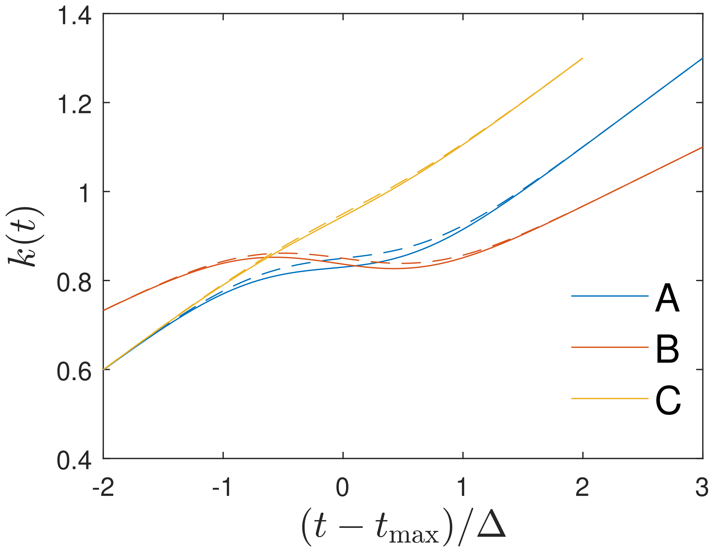
3. Condition for the Validity of the Gaussian Evolution

In this Section, the Gaussian evolution is adopted for the rate of new infections [40,41]:
J ˙ ( t ) = J π Δ exp ( t t max ) 2 Δ 2 .
The corresponding accumulative fraction of infections at any time then is given by
J ( t ) = t d t e ( t t max ) 2 Δ 2 = J 2 1 + erf t t max Δ ,
in terms of the error function. J denotes the final cumulative fraction of infections after infinite time, t . The Gaussian evolution (21) implies:
J ¨ ( t ) = 2 ( t t max ) Δ 2 J ˙ ( t ) .
In the general case of arbitrarily large J , the full Equation (16) yields for the Gaussian evolution,
k ( t ) = 1 J 2 1 + erf t t max Δ + 2 ( t t max ) a 0 Δ 2 J e ( t t max ) 2 Δ 2 π a 0 Δ 1 J 2 1 + erf t t max Δ .
In the limit J 1 , as also indicated by the first Equation (20), the last term in Equation (24) is negligibly small providing in this limit:
k ( t ) 1 J 2 1 + erf t t max Δ + 2 ( t t max ) a 0 Δ 2 .
The full ratio (24) and its approximation (25) are shown in Figure 1. One notices that the approximation (25) agrees well enough with the exact time variation (24). As one can see, Figure 1 indicates three different regimes in time for the Gaussian ratio:
(i)
at early times t t max , the Gaussian ratio increases linearly starting from ratio values less than unity;
(ii)
at times near maximum, i.e., close to t max near the maximum of J ˙ ( t ) , the Gaussian ratio exhibits a dip, which is more pronounced for smaller values of a 0 and which is also indicated by Equation (25) as the third linear term is inversely proportional to a 0 ;
(iii)
at late times beyond t max , the Gaussian ratio resumes its linear increase with time.
We conclude that for the time dependency (24) of the ratio k ( t ) , the Gaussian evolution (21) is an exact analytical solution of the SIR equations. Likewise, if the monitored differential, J ˙ ( t ) , and cumulative, J ( t ) , infection rates inserted in Equation (16) are well approximated by the Gaussian ratios (24) and (25) in all three distinct time regimes, one can justify the use the Gaussian evolution (21) as good approximations of the solutions of the SIR equations.

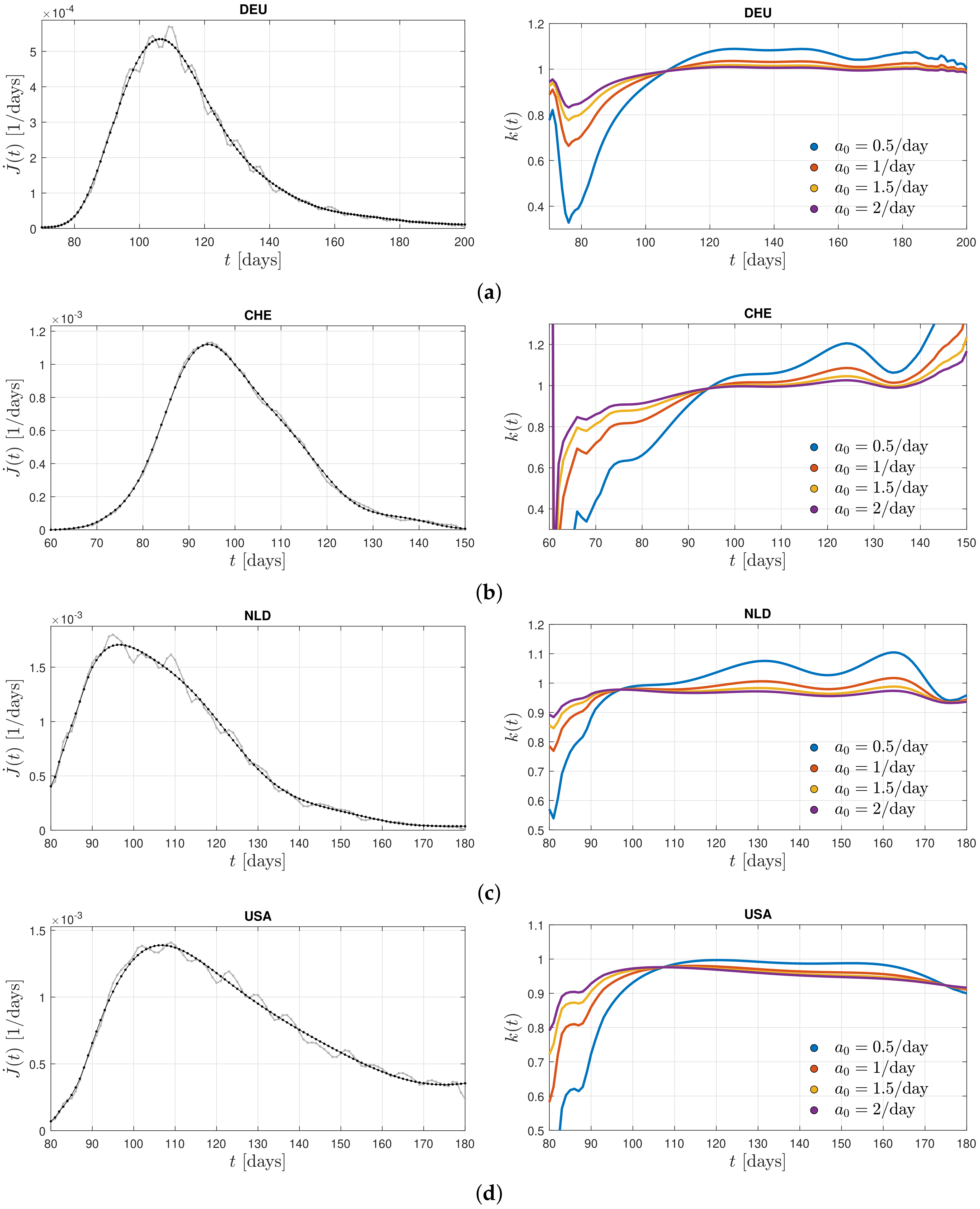
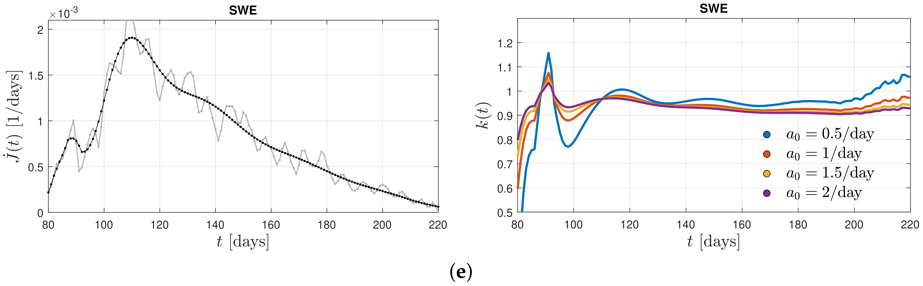
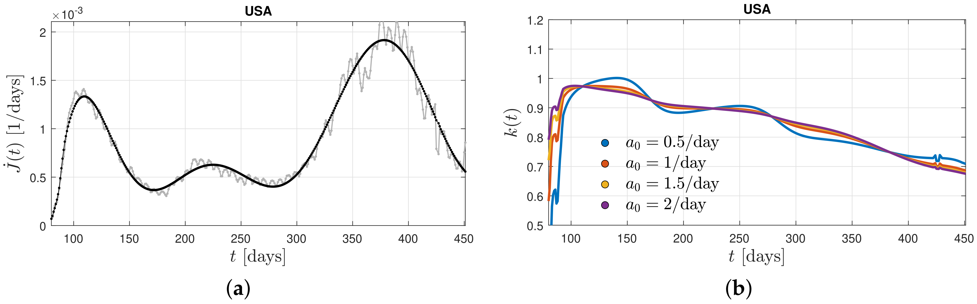
4. Determination of Ratio (16) from Monitored Infection Rates of COVID-19 Waves

Figure 2, left, shows the differential infection rate, J ˙ ( t ) , in the five countries such as Germany, Switzerland, the Netherlands, the United States, and Sweden inferred from the reported death rates [43] adopting a fatality rate of 0.005. In each country, the raw data (in grey) were smoothed (black curves) in order to infer the second derivative, J ¨ ( t ) . Figure 2, left, shows the derived ratio, k ( t ) , calculated from Equation (20) for different values of the stationary infection rate, a 0 .
The monitored infection rates exhibit one well pronounced maximum during the selected time spans capturing a single wave. Remarkably, corresponding inferred ratios k ( t ) in these countries show quite similar behavior. In all cases, except Sweden, one notices a linear increase at early times below the first maximum of J ˙ ( t ) before the ratios approach a nearly constant value close to unity at the time of the first maximum with small amplitude oscillations at later times. A resumed linear increase in the ratio at late times is not visible. Consequently, one can conclude that the Gaussian evolution (21) provides a good approximation of the solutions of the SIR equations during early and peak times. It, however, fails at late times beyond the first maximum of the considered past corona waves in these five countries. This good agreement of the Gaussian modeling at times prior the maximum in the monitored differential infection rates justifies a posteriori the earlier approaches [38,39,40,41]. Moreover, the almost constant values of the ratio k ( t ) at times after the maximum time indicate that the analytical SIR solutions [35,36] based on a constant ratio are decently applicable at these times.
Common to all five examples, shown in Figure 1, is that only one pronounced maximum in the differential rate of new infections is visible. Figure 3 shows the differential rate of new infections on longer time scales in the United States. Here, at least three maxima are exhibited so that the ratio k ( t ) at late times deviates from its nearly constant value and decreases substantially with time. This well demonstrates that a ratio k ( t ) decreasing to values considerably less than unity is responsible for leading to new maxima in the rate of new infections of the same mutant.
It needs to be emphasized (We are grateful to one of the referees for noting this point) that the deductions on the time dependence of the parameter k ( t ) here are most appropriate for populations with expectedly relatively homogenous pandemic dynamics in Germany, Switzerland, the Netherlands, and Sweden, where in particular non-pharmaceutical interventions and/or vaccination campaigns have been applied uniformly and simultaneously countrywide. In contrast, for the United States, with its diversified and non-uniformly applied local control measures, in some cases ranging from near total quarantine to near total reopening, it is unlikely that the different peaks of the differential infection rate shown in Figure 3, indeed resulted from a single starting point in time. Here, a more distributed approach for such large countries with diversified local control measures seems to be necessary. Relevant work has considered that the interconnection pattern in large countries like the United States follows rather a hierarchical “network of networks” topology (see, e.g., [44,45]). In this case, the countrywide wave would then consist of multiple local waves, which can be shifted in time and thus also in the phase of the epidemic wave.
As a consequence for such large countries as the United States, one would expect something like a superposition of SIR models with different starting points and thus with different weight distributions at any given point of time, that in turn is typically reflected by heavy-tailed patterns in the marginal distributions, as happens in diffusion models and could be observed in various complex systems with spatio-temporal propagation ranging from train delays to biomolecular dynamics [46,47,48,49,50,51,52]. Thus, for prediction making, these “local” models can be updated based on their interconnection patterns with other “local” models (for an example of a seemingly relevant approach, see, e.g., [53]).

5. Summary and Conclusions

The SIR-epidemic model provides a good explanation for the temporal evolution of COVID-19 waves from different mutants. An important key parameter of the SIR model is the ratio k ( t ) = μ ( t ) / a ( t ) of the recovery to infection rate. Here, apparently for the first time, monitored differential infection rates of past corona waves have been used to infer a posteriori the real time variation of this key parameter. By attributing its time dependence formally to a time-dependent recovery rate the temporal evolution of the ratio k ( t ) is inferred for different values of the stationary infection rate a 0 .
For past corona waves in five different countries, it is found that the ratio k ( t ) exhibits a linear increase at early times below the first maximum of the differential infection rate before the ratio approaches a nearly constant value close to unity at the time of the first maximum with small amplitude oscillations at later times. The deductions on the time dependence of the parameter k ( t ) are most appropriate for populations with expectedly relatively homogenous pandemic dynamics such as in Germany, Switzerland, the Netherlands and Sweden where in particular non-pharmaceutical interventions have been applied uniformly and simultaneously countrywide.
The observed time dependencies at early times and at times near the first maximum agree favorably well with the behavior of the calculated ratio k ( t ) for the Gaussian evolution for the rate of new infections, although the predicted linear increase in the Gaussian ratio at late times is not observed.
Likewise, the near constancy of the ratio k ( t ) at times after the maximum time indicates that earlier analytical solutions of the SIR equations for constant ratios are well justified.
On longer time intervals, more than one maximum in the differential rate of new infections indicates the presence of several maxima which can be explained by a decrease in the ratio k ( t ) at times after the first maximum to values considerably less than unity. This decrease then is responsible for causing new maxima in the rate of new infections of the same mutant.

Author Contributions

Conceptualization, R.S.; methodology, R.S. and M.K.; software, M.K.; writing—original draft preparation, R.S.; writing—review and editing, R.S. and M.K.; visualization, M.K. All authors have read and agreed to the published version of the manuscript.

Funding

This research received no external funding.

Data Availability Statement

The raw, real-time data used in this study has been retrieved from Ref. [43].

Conflicts of Interest

The authors declare no conflict of interest.

References

  1. Kermack, W.O.; McKendrick, A.G. A contribution to the mathematical theory of epidemics. Proc. R. Soc. A Math. Phys. Engin. Sci. 1927, 115, 700–721. [Google Scholar] [CrossRef]
  2. Kendall, D.G. Deterministic and stochastic epidemics in closed populations. In Proceedings of the Third Berkeley Symposium on Mathematical Statistics and Probability. Volume 4: Contributions to Biology and Problems of Health; Neyman, J., Ed.; University of California Press: Berkeley/Los Angeles, CA, USA, 1956; pp. 149–166. [Google Scholar] [CrossRef]
  3. Annas, S.; Pratama, M.I.; Rifandi, M.; Sanusi, W.; Side, S. Stability analysis and numerical simulation of SEIR model for pandemic COVID-19 spread in Indonesia. Chaos Solit. Fract. 2020, 139, 110072. [Google Scholar] [CrossRef]
  4. Hou, C.; Chen, J.; Zhou, Y.; Hua, L.; Yuan, J.; He, S.; Guo, Y.; Zhang, S.; Jia, Q.; Zhao, C.; et al. The effectiveness of quarantine of Wuhan city against the Corona Virus Disease 2019 (COVID-19): A well-mixed SEIR model analysis. J. Med. Virol. 2020, 92, 841–848. [Google Scholar] [CrossRef]
  5. Yang, Z.; Zeng, Z.; Wang, K.; Wong, S.S.; Liang, W.; Zanin, M.; Liu, P.; Cao, X.; Gao, Z.; Mai, Z.; et al. Modified SEIR and AI prediction of the epidemics trend of COVID-19 in China under public health interventions. J. Thorac. Dis. 2020, 12, 165–174. [Google Scholar] [CrossRef] [PubMed]
  6. He, S.; Peng, Y.; Sun, K. SEIR modeling of the COVID-19 and its dynamics. Nonlin. Dyn. 2020, 101, 1667–1680. [Google Scholar] [CrossRef] [PubMed]
  7. Rezapour, S.; Mohammadi, H.; Samei, M.E. SEIR epidemic model for COVID-19 transmission by Caputo derivative of fractional order. Adv. Diff. Equ. 2020, 2020, 490. [Google Scholar] [CrossRef]
  8. Ghostine, R.; Gharamti, M.; Hassrouny, S.; Hoteit, I. An extended SEIR model with vaccination for forecasting the COVID-19 pandemic in Saudi Arabia using an ensemble Kalman filter. Mathematics 2021, 9, 636. [Google Scholar] [CrossRef]
  9. Berger, D.; Herkenhoff, K.; Huang, C.; Mongey, S. Testing and reopening in an SEIR model. Rev. Econ. Dyn. 2022, 43, 1–21. [Google Scholar] [CrossRef]
  10. Engbert, R.; Rabe, M.M.; Kliegl, R.; Reich, S. Sequential data assimilation of the stochastic SEIR epidemic model for regional COVID-19 dynamics. Bull. Math. Biol. 2021, 83, 1. [Google Scholar] [CrossRef]
  11. Bentout, S.; Chen, Y.; Djilali, S. Global dynamics of an SEIR model with two age structures and a nonlinear incidence. Acta Appl. Math. 2021, 171, 7. [Google Scholar] [CrossRef]
  12. Carcione, J.M.; Santos, J.E.; Bagaini, C.; Ba, J. A simulation of a COVID-19 epidemic based on a deterministic SEIR model. Front. Publ. Health 2020, 8, 230. [Google Scholar] [CrossRef]
  13. Nabti, A.; Ghanbari, B. Global stability analysis of a fractional SVEIR epidemic model. Math. Meth. Appl. Sci. 2021, 44, 8577–8597. [Google Scholar] [CrossRef]
  14. Lopez, L.; Rodo, X. A modified SEIR model to predict the COVID-19 outbreak in Spain and Italy: Simulating control scenarios and multi-scale epidemics. Results Phys. 2021, 21, 103746. [Google Scholar] [CrossRef]
  15. Korolev, I. Identification and estimation of the SEIRD epidemic model for COVID-19. J. Econom. 2021, 220, 63–85. [Google Scholar] [CrossRef]
  16. Jahanshahi, H.; Munoz-Pacheco, J.M.; Bekiros, S.; Alotaibi, N.D. A fractional-order SIRD model with time dependent memory indexes for encompassing the multi-fractional characteristics of the COVID-19. Chaos Solit. Fract. 2021, 143, 110632. [Google Scholar] [CrossRef]
  17. Nisar, K.S.; Ahmad, S.; Ullah, A.; Shah, K.; Alrabaiah, H.; Arfan, M. Mathematical analysis of SIRD model of COVID-19 with Caputo fractional derivative based on real data. Results Phys. 2021, 21, 103772. [Google Scholar] [CrossRef]
  18. Faruk, O.; Kar, S. A Data driven analysis and forecast of COVID-19 dynamics during the third wave using SIRD model in Bangladesh. COVID 2021, 1, 503–517. [Google Scholar] [CrossRef]
  19. Rajasekar, S.P.; Pitchaimani, M. Ergodic stationary distribution and extinction of a stochastic SIRS epidemic model with logistic growth and nonlinear incidence. Appl. Math. Comput. 2020, 377, 125143. [Google Scholar] [CrossRef]
  20. Hu, H.; Yuan, X.; Huang, L.; Huang, C. Global dynamics of an SIRS model with demographics and transfer from infectious to susceptible on heterogeneous networks. Math. Biosci. Engin. 2019, 16, 5729–5749. [Google Scholar] [CrossRef]
  21. Babaei, N.A.; Özer, T. On exact integrability of a COVID-19 model: SIRV. Math. Meth. Appl. Sci. 2023. Early View. [Google Scholar] [CrossRef]
  22. Rifhat, R.; Teng, Z.; Wang, C. Extinction and persistence of a stochastic SIRV epidemic model with nonlinear incidence rate. Adv. Diff. Equ. 2021, 2021, 200. [Google Scholar] [CrossRef]
  23. Ameen, I.; Baleanu, D.; Ali, H.M. An efficient algorithm for solving the fractional optimal control of SIRV epidemic model with a combination of vaccination and treatment. Chaos Solit. Fract. 2020, 137, 109892. [Google Scholar] [CrossRef]
  24. Oke, M.O.; Ogunmiloro, O.M.; Akinwumi, C.T.; Raji, R.A. Mathematical modeling and stability analysis of a SIRV epidemic model with non-linear force of infection and treatment. Commun. Math. Appl. 2019, 10, 717–731. [Google Scholar] [CrossRef]
  25. Keeling, M.J.; Rohani, P. Modeling Infectious Diseases in Humans and Animals; Princeton University Press: Princeton, NJ, USA, 2008. [Google Scholar] [CrossRef]
  26. Estrada, E. COVID-19 and SARS-CoV-2. Modeling the present, looking at the future. Phys. Rep. 2020, 869, 1–51. [Google Scholar] [CrossRef]
  27. Lopez, L.; Rodo, X. The end of social confinement and COVID-19 re-emergence risk. Nat. Hum. Behav. 2020, 4, 746–755. [Google Scholar] [CrossRef]
  28. Miller, I.F.; Becker, A.D.; Grenfell, B.T.; Metcalf, C.J.E. Disease and healthcare burden of COVID-19 in the United States. Nat. Med. 2020, 26, 1212–1217. [Google Scholar] [CrossRef]
  29. Reiner, R.C., Jr.; Barber, R.M.; Collins, J.K.; Zheng, P.; Adolph, C.; Albright, J.; Antony, C.M.; Aravkin, A.Y.; Bachmeier, S.D.; Bang-Jensen, B.; et al. Modeling COVID-19 scenarios for the United States. Nat. Med. 2021, 27, 94–105. [Google Scholar] [CrossRef]
  30. Linka, K.; Peirlinck, M.; Sahli Costabal, F.; Kuhl, E. Outbreak dynamics of COVID-19 in Europe and the effect of travel restrictions. Comp. Meth. Biomech. Biomed. Eng. 2020, 23, 710–717. [Google Scholar] [CrossRef]
  31. Filindassi, V.; Pedrini, C.; Sabadini, C.; Duradoni, M.; Guazzini, A. Impact of COVID-19 first wave on psychological and psychosocial dimensions: A systematic review. COVID 2022, 2, 273–340. [Google Scholar] [CrossRef]
  32. Postnikov, E.B. Estimation of COVID-19 dynamics “on a back-of-envelope”: Does the simplest SIR model provide quantitative parameters and predictions? Chaos Solit. Fract. 2020, 135, 109841. [Google Scholar] [CrossRef]
  33. Cooper, I.; Mondal, A.; Antonopoulos, C.G. A SIR model assumption for the spread of COVID-19 in different communities. Chaos Solit. Fract. 2020, 139, 110057. [Google Scholar] [CrossRef]
  34. Hespanha, J.P.; Chinchilla, R.; Costa, R.R.; Erdal, M.K.; Yang, G. Forecasting COVID-19 cases based on a parameter-varying stochastic SIR model. Annu. Rev. Control 2021, 51, 460–476. [Google Scholar] [CrossRef]
  35. Kröger, M.; Schlickeiser, R. Analytical solution of the SIR-model for the temporal evolution of epidemics. Part A: Time-independent reproduction factor. J. Phys. A Math. Theor. 2020, 53, 505601. [Google Scholar] [CrossRef]
  36. Schlickeiser, R.; Kröger, M. Analytical solution of the SIR-model for the temporal evolution of epidemics: Part B. Semi-time case. J. Phys. A Math. Theor. 2021, 54, 175601. [Google Scholar] [CrossRef]
  37. Kröger, M.; Schlickeiser, R. SIR-solution for slowly time dependent ratio between recovery and infection rates. Physics 2022, 4, 504–524. [Google Scholar] [CrossRef]
  38. Ciufolini, I.; Paolozzi, A. Mathematical prediction of the time evolution of the COVID-19 pandemic in Italy by a Gauss error function and Monte Carlo simulations. Eur. Phys. J. Plus 2020, 135, 355. [Google Scholar] [CrossRef]
  39. Li, L.; Yang, Z.; Deng, Z.; Meng, C.; Huang, J.; Meng, H.; Wang, D.; Chen, G.; Zhang, J.; Peng, H.; et al. Propagation analysis and prediction of the COVID-19. Infect. Disease Model. 2020, 5, 282–292. [Google Scholar] [CrossRef]
  40. Schlickeiser, R.; Schlickeiser, F. A Gaussian model for the time development of the SARS-CoV-2 corona pandemic disease. Prrdictions for Germany made on 30 March 2020. Physics 2020, 2, 164–170. [Google Scholar] [CrossRef]
  41. Schüttler, J.; Schlickeiser, R.; Schlickeiser, F.; Kröger, M. COVID-19 predictions using a Gauss model, based on data from April 2. Physics 2020, 2, 197–212. [Google Scholar] [CrossRef]
  42. Kröger, M.; Schlickeiser, R. Verification of the accuracy of the SIR model in forecasting based on the improved SIR model with a constant ratio of recovery to infection rate by comparing with monitored second wave data. R. Soc. Open Sci. 2021, 8, 211379. [Google Scholar] [CrossRef] [PubMed]
  43. Dong, E.; Du, H.; Gardner, L. An interactive web-based dashboard to track COVID-19 in real time. Lancet Infect. Disease 2020, 20, 533–534. [Google Scholar] [CrossRef]
  44. Gao, J.; Buldyrev, S.V.; Havlin, S.; Stanley, H.E. Robustness of a network of networks. Phys. Rev. Lett. 2011, 107, 195701. [Google Scholar] [CrossRef] [PubMed]
  45. Gao, J.; Li, D.; Havlin, S. From a single network to a network of networks. Natl. Sci. Rev. 2014, 1, 346–356. [Google Scholar] [CrossRef]
  46. Beck, C.; Cohen, E.G.D. Superstatistics. Phys. A Stat. Mech. Appl. 2003, 322, 267–275. [Google Scholar] [CrossRef]
  47. Beck, C. Stretched exponentials from superstatistics. Phys. A Stat. Mech. Appl. 2006, 365, 96–101. [Google Scholar] [CrossRef]
  48. Briggs, K.; Beck, C. Modelling train delays with q-exponential functions. Phys. A Stat. Mech. Appl. 2007, 378, 498–504. [Google Scholar] [CrossRef]
  49. Tamazian, A.; Nguyen, V.D.; Markelov, O.A.; Bogachev, M.I. Universal model for collective access patterns in the Internet traffic dynamics: A superstatistical approach. EPL (Europhys. Lett.) 2016, 115, 10008. [Google Scholar] [CrossRef]
  50. Bogachev, M.I.; Markelov, O.A.; Kayumov, A.R.; Bunde, A. Superstatistical model of bacterial DNA architecture. Sci. Rep. 2017, 7, 43034. [Google Scholar] [CrossRef] [Green Version]
  51. Metzler, R. Superstatistics and non-Gaussian diffusion. Eur. Phys. J. Spec. Top. 2020, 229, 711–728. [Google Scholar] [CrossRef]
  52. Itto, Y.; Beck, C. Superstatistical modelling of protein diffusion dynamics in bacteria. J. R. Soc. Interface 2021, 18, 20200927. [Google Scholar] [CrossRef]
  53. Mark, C.; Metzner, C.; Lautscham, L.; Strissel, P.L.; Strick, R.; Fabry, B. Bayesian model selection for complex dynamic systems. Nat. Commun. 2018, 9, 1803. [Google Scholar] [CrossRef] [PubMed] [Green Version]
Figure 1. The Gaussian ratio (24) (full curves) and its approximation (25) (dashed curves) plotted for the three cases (A) a 0 = 1 days 1 , J = 0.3 , Δ = 10 days, (B) a 0 = 0.5 days 1 , J = 0.3 , Δ = 30 days and (C) a 0 = 0.5 days 1 , J = 0.1 , Δ = 20 days, respectively. See text for details.
Physics 05 00016 g001
Figure 2. Left: differential infection rate, J ˙ ( t ) . The raw data (in grey) are smoothed (black curve) in order to infer the second derivative, J ¨ ( t ) . Right: the derived ratio, k ( t ) (see Equation (20)) for different values of the stationary infection rate, a 0 . The data are inferred from the reported death rates [43] adopting a fatality rate of 0.005 for (a) Germany, from the first corona wave during days 70–200 (March 10–July 18) in the year 2020, (b) Switzerland, during days 60–150, (c) the Netherlands, during days 80–180, (d) the United States, during days 80–180, and (e) Sweden, during days 80–220, where day 1 is 1 January 2020 in (be).
Physics 05 00016 g002aPhysics 05 00016 g002b
Figure 3. (a) Differential infection rate, J ˙ ( t ) , in the United States, from the first three corona waves during days 80–450 (20 March 2020–24 March 2021) inferred from the reported death rates [43] adopting a fatality rate of 0.005. The raw data (in grey) are smoothed (black curve) in order to infer the second derivative, J ¨ ( t ) . (b) The derived ratio, k ( t ) (see Equation (20)), for different values of the stationary infection rate, a 0 .
Physics 05 00016 g003
Disclaimer/Publisher’s Note: The statements, opinions and data contained in all publications are solely those of the individual author(s) and contributor(s) and not of MDPI and/or the editor(s). MDPI and/or the editor(s) disclaim responsibility for any injury to people or property resulting from any ideas, methods, instructions or products referred to in the content.

