Review

Recent Progress of Shell-Model Calculations, Monte Carlo Shell Model, and Quasi-Particle Vacua Shell Model

by
Noritaka Shimizu
1,2
1
Center for Computational Sciences and Faculty of Pure and Applied Sciences, University of Tsukuba, 1-1-1 Tennodai, Tsukuba 305-8577, Japan
2
Center for Nuclear Study, The University of Tokyo, 7-3-1, Hongo, Bunkyo-ku, Tokyo 113-0033, Japan
Physics 2022, 4(3), 1081-1093; https://doi.org/10.3390/physics4030071
Submission received: 31 July 2022 / Revised: 23 August 2022 / Accepted: 25 August 2022 / Published: 9 September 2022

Abstract

:
Nuclear shell model is a powerful approach to investigate nuclear structure microscopically. However, the computational cost of shell-model calculations becomes huge in medium-heavy nuclei. I briefly review the theoretical framework and the code developments of the conventional Lanczos diagonalization method for shell-model calculations. In order to go beyond the conventional diagonalization method, the Monte Carlo shell model and the quasiparticle-vacua shell model were introduced. I present some benchmark examples of these models.

1. Introduction

Nuclear shell-model calculation is often called the “configuration interaction” (CI) method in analogy to the CI method in quantum chemistry. It provides us with a detailed description of the ground and low-lying excited states of medium-mass nuclei [1]. A shell-model study is an excellent theoretical tool to discuss exotic structures of nuclei, such as the shape coexistence, shape phase transition, emergence of new magic numbers in neutron-rich nuclei, and so on [1,2]. In addition, it enables us to predict nuclear data required for astrophysical applications [3,4] and for elementary particle physics [5,6,7,8]. In the shell-model framework, one separates a nuclear wave function into two parts: an inert core and active particles in the model space. Usually, an inert core is taken as a doubly magic nucleus closest to the Fermi level. For example, in the case of 48 Ca, 40 Ca ( N = Z = 20 , where N denotes the number of neutrons and Z the number of protons in a nucleus) is taken as a frozen inert core and eight valence neutrons are actively occupying the p f -shell orbits. Its wave function is written as a linear combination of the Slater determinants each of which represents how the active particles occupy single-particle orbits. This model has achieved successful description of p-shell [9], s d -shell [10], p f -shell, [1,11,12], and f 5 p g 9 -shell [13] nuclei with the conventional diagonalization method.
In most of the conventional shell-model studies, the shell-model Hamiltonian is constructed by the many-body perturbation theory [14] with minor phenomenological corrections to fit the experimental data. Its ab initio derivation has been recently developed by the valence-space in-medium similarity renormalization group (VS-IMSRG) method [15], the coupled-cluster method [16], the many-body perturbation theory [17], the extended Krenciglowa–Kuo method [18], and Okubo–Lee–Suzuki approach [19], while ab initio description of strongly quadrupole deformed states is still a challenge [15,20,21]. The shell-model calculation is now applied to ab initio theory and its importance increases now.
However, solving the eigenvalue problem of the shell-model Hamiltonian matrix often requires huge computational resources, which hampers us from performing the shell-model study in the whole nuclear region. Moreover, in the case of neutron-rich nuclei, since the proton and neutron Fermi levels locate in different shells, beyond one-major-shell model space is required for such model space and the exact diagonalization is often infeasible. To circumvent this problem, Tokyo shell-model group introduced the Monte Carlo shell model (MCSM), which provides us with successful description of medium-mass nuclei [22,23]. For heavy nuclei in which the treatment of the pairing correlation is important, the MCSM is not sufficiently efficient and its extension, quasi-particle vacua shell model (QVSM), was introduced [24].
In this paper, I briefly describe the framework of the shell-model calculations and the developments of the shell-model codes in Section 2. In Section 3, various approximation methods going beyond the limitation of the conventional shell-model diagonalization are reviewed. Among them, the MCSM is discussed in Section 3.1. Section 3.2 is devoted to the description of the QVSM framework and its capability. This paper is summarized in Section 4.

2. Conventional Diagonalization Method for Shell-Model Calculations

In this Section, I briefly review computational aspects of conventional shell-model calculations with the Lanczos method and the developments of shell-model codes.

2.1. Shell-Model Hamiltonian Matrix and Its Dimension

A shell-model Hamiltonian consists of one-body and two-body interactions as
H = i ϵ i c i c i + i j k l v i j k l c i c j c l c k ,
where c i ( c i ) denote the annihilation (creation) operator of the single-particle state i. ϵ i and v i j k l are the single-particle energies (SPEs) and the two-body matrix elements (TBMEs), respectively, which are fixed so that rotational and parity symmetries are kept. In a conventional way, the SPEs and TBMEs are determined based on the many-body perturbation theory and are corrected phenomenologically so that the experimental binding energies and excitation energies are reproduced. In the so-called M-scheme framework, the shell-model wave function is written as a linear combination of the vast number of the M-scheme basis states as
| Ψ = α = 1 D v α | M α ,
| M α = i = 1 A c α i | ,
where { α i } is a set of the single-particle orbits occupied by the active particles. The symbol | denotes the wave function of the inert core. D is the number of the basis states allowed with a specified z-component of the angular momentum (M) and parity ( π ), and called the “M-scheme dimension”. The Schrödinger equation is reduced to the eigenvalue problem:
β = 1 D M α | H | M β v β = E v α .
Here, E denotes an eigenvalue of the Hamiltonian matrix, M α | H | M β .
What a shell-model code does is to solve the eigenvalue problem in Equation (4) and obtain a few numbers of the lowest eigenvalues and their eigenvectors with the Lanczos method. Since the M-scheme basis state | M α is not an eigenstate of the total angular momentum, J 2 , the wave function in Equation (2) is generally not an eigenstate of J 2 . However, since the shell-model Hamiltonian is commutable with J 2 , the solution obtained by the Lanczos method automatically becomes an eigenstate of J 2 in the case without any degeneracy. On the other hand, a j j -coupled basis state with a good J 2 eigenvalue can be constructed with additional angular-momentum algebra. Such basis state is called a “J-scheme basis state” and the number of the allowed J-scheme basis states is called the “J-scheme dimension”.
Table 1 shows the shell-model dimensions of several example nuclei with one-major-shell model space. Since the current limitation of the M-scheme dimension is around 10 11 10 12 , nuclei with the f 5 p g 9 model space and nuclei in the smaller mass region are able to be handled. Most open-shell heavy nuclei with the atomic mass number A > 100 are still far beyond the current capability. Since the numerical size of a vector with the M-scheme dimension D is 8 D Byte for the double precision, the capacity of the disk and memory restricts the capability. The dimensions of the J-scheme basis states are also shown in Table 1. It is two orders of magnitude smaller than the corresponding M-scheme dimensions. However, the M-scheme Hamiltonian matrix is simpler and more sparse than the J-scheme Hamiltonian matrix and then the M-scheme basis state is used for many numerical computations.
In order to perform shell-model calculations in medium-heavy nuclei with huge dimensions, various shell-model codes were developed. One of the most famous, popular shell-model codes is the MSU (Michigan State University) version of the OXBASH code [25,26], which was published in the 1980s. Its algorithm is a hybrid method combining M-scheme and J-scheme basis states. It is equipped with a dialogue-type user-friendly interfaced and had been most widely used in the nuclear physics community. It was replaced in the 2010s by its successor, NuShellX@MSU [27]. On the other hand, the M-scheme ANTOINE code and its cousin, the J-scheme NATHAN code were developed by Strasbourg-Madrid shell-model group [28,29]. The ANTOINE code has also been used in various studies. It is equipped with an efficient algorithm based on on-the-fly generation of the coupling of the proton and neutron basis states [1] and heavily relies on the FORTRAN 77 language. The MSHELL and MSHELL64 codes were developed mainly by T. Mizusaki [30,31].
A recent major trend in the high-performance computing environment is massively parallel computation. In order to perform shell-model calculations on modern massively parallel computers efficiently, several shell-model codes have been developed recently, such as the MFDn [32], BIGSTICK [33], and KSHELL [34] codes. Among them, the KSHELL code was developing, which is equipped with MPI (Message Passing Interface)–OpenMP (Open Multi-Processing) hybrid parallel computation and can be used both in a personal computer and state-of-the-art supercomputer in the same manner. It shows good parallel scaling up to around 10 4 threads [34]. The MFDn and BIGSTICK codes are mainly oriented to the no-core shell-model approach by including three-body forces explicitly.

2.2. Lanczos Method

The Lanczos method [35] is one of the simplest Krylov subspace methods, in which the low-lying exact eigenvalues are approximated by the Ritz values of the Krylov subspace. The Krylov subspace is spanned by an initial vector, v 0 , and its vector multiplied by the shell-model Hamiltonian matrix as
K n ( H , v 0 ) = span { v 0 , H v 0 , H 2 v 0 , , H n 1 v 0 } .
The exact eigenvalues are approximated by the eigenvalues of the Hamiltonian matrix in the subspace K n ( H , v 0 ) . In the Lanczos method one performs the orthonormalization of the vector at every n, which makes the method numerically stable. While in the limit of n D the approximated eigenvalues agree with the exact ones, a few of the smallest eigenvalues converge with small n, typically n 300 to obtain the 10 lowest eigenvalues [36]. In practical codes, its extension, the thick-restart Lanczos method, is widely used [37].

2.3. Block Lanczos Method

In a large-scale problem, the number of the Hamiltonian matrix elements is too huge to be stored in the memory. In the KSHELL code, the product of the Hamiltonian matrix and a vector is the most time-consuming part of the Lanczos algorithm, since the Hamiltonian matrix elements are generated on-the-fly for every matrix-vector product. In order to reduce the time of the on-the-fly generation, the block algorithm to the thick-restart Lanczos method, named the thick-restart block Lanczos method [34].
In the block algorithm, the on-the-fly generation is performed on every product of the matrix and block vectors, not a vector. Since the number of the products in the block Lanczos method is usually much smaller than that in the Lanczos method, the number of the generations is reduced in comparison with the Lanczos method. The block Lanczos method is one of the block Krylov subspace methods. The block Krylov subspace is defined with a block of the initial vectors V 0 = ( v 0 , 1 , v 0 , 2 , v 0 , q ) as
K n ( H , V 0 ) = span { V 0 , H V 0 , H 2 V 0 , , H n 1 V 0 } ,
where q is the block size. Although this subspace is spanned by the n q vectors the number of on-the-fly generation of the matrix elements is n. The eigenvalues of the Hamiltonian in the Krylov block subspace are a good approximation to the exact ones. In practical code, the thick-restart block Lanczos method was introduced in the KSHELL code [34].
As other eigensolvers for the shell-model calculations, the LOBPCG method [38] and the Sakurai–Sugiura method [39] have been tested. In our KSHELL code, the block Sakurai–Sugiura method and its variant, stochastic estimation of eigenvalue density, were also implemented [40,41]. To study resonance states such as the Gamow shell model, the energies of the target many-body resonant states correspond to interior eigenvalues, not the lowest one, and are complex numbers. Since the simple Lanczos method cannot be used in such a case, the Jacobi-Davidson method was adopted in the Gamow shell model [42] and the Sakurai–Sugiura method was tested in the complex scaling method [43].

3. Approximation Methods to Exact Diagonalization

While shell-model codes for large-scale calculations have been developed vigorously, various approximation schemes to the full model space were proposed. I briefly review these attempts hereafter.
The auxiliary-field Monte Carlo was applied to shell-model calculations and became one of the successful methods in describing p f -shell nuclei in the 1990s [44]. However, the notorious sign problem in the quantum Monte Carlo method hampers us from utilizing realistic effective interactions. As a possible solution to the sign problem, the extrapolation method [44], the complex Langevin method [45], and a constrained-path approximation [46] were suggested. Rather schematic interaction without the sign problem has been adopted for the study of nuclear level density [47].
The density matrix renormalization group (DMRG) method is known to be an efficient variational method to solve a one-dimensional quantum many-body problem. It was applied to shell-model calculations coupled to continuum states [48,49]. Its advanced one, the tensor network method, was applied later [50]. The projected shell model has been a useful model with rather schematic interaction to describe high-spin states [51]. The angular-momentum projected CI is another variational method whose basis states are the angular-momentum projected deformed Slater determinants with particle-hole excitation [52]. On top of that, a lot of effort has been paid to developing efficient truncation schemes, such as the correlated basis method [53], the variational Monte Carlo method with random walkers in M-scheme basis states [54,55], nucleon-pair truncation [56,57], generator coordinate method (GCM) [58] and so on.
The variation after mean-field projection in realistic model space (VAMPIR) method is one of the successful methods to describe the N Z medium-mass nuclei [59,60]. In the VAMPIR method, the nuclear wave function is expressed as a linear combination of the parity, angular-momentum, number projected quasiparticle vacua. Each basis state is determined one by one by minimizing the energy expectation value of this wave function. In that sense, this method is the variation after the projection and superposition. In the hybrid multi-determinant (HMD) method, the number-projected quasiparticle vacua are replaced by the deformed Slater determinants [61,62]. The HMD has been used mainly for the no-core shell-model approach [63].
These truncation methods provide us with the variational upper limit, which may be controlled by a parameter to define the truncation. The exact energy can be estimated by the extrapolation of the energy function of this parameter. The exponential convergence method was suggested, the energy eigenvalue of the truncated subspace is expected to converge as a function of its dimension [64]. As an alternative, the energy-variance expectation value of the variational wave function can be used as a parameter for extrapolation. The energy function of the energy variance can be fitted as a polynomial function, which enables us to estimate the exact energy precisely. It was first introduced into the shell-model calculation with particle-hole truncation in Ref. [65] and applied also to no-core shell model calculations [66], the MCSM [67], QVSM [24], HMD [68], and the importance-truncated shell model (ITSM) [69].
The ITSM was introduced firstly into the no-core shell model approach by R. Roth and his collaborators successfully [70], and later applied also to the conventional shell model approach [69]. The M-scheme basis states are truncated by the importance measure, which is estimated by the many-body perturbation theory. The energy is calculated as a function of the criteria of the importance measure, and it is extrapolated to the full space. One of its results is shown in Section 3.2.
Among these efforts, the MCSM and the QVSM have been introduced. These models are discussed in the following Subsections.

3.1. Monte Carlo Shell Model

Among all the efforts to develop various approximation schemes, the MCSM was suggested in the 1990s [22,71,72] and revised in an advanced form [23,73] in the 2010s. It has been used for extensive studies of neutron-rich nuclei. In this Section, I briefly review the theoretical framework of the MCSM.
In the MCSM the nuclear wave function is written as a linear combination of the parity, angular-momentum projected deformed Slater determinants:
| Ψ ( N b ) = n = 1 N b K = J J f n K P M K J π | ϕ n .
| ϕ n is a deformed Slater determinant given as
| ϕ n = α k D k α ( n ) c k | ,
which is parametrized by the complex matrix D k α ( n ) . The energy E ( N b ) is provided by solving the following generalized eigenvalue problem of the Hamiltonian and norm matrices:
n K H m M , n K f n K = E ( N b ) n K H m M , n K f n K , H m M , n K = ϕ m | H P M K J π | ϕ n , N m M , n K = ϕ m | P M K J π | ϕ n ,
where P M K J π is the angular-momentum (J), parity ( π ) projector. f i K is the corresponding eigenvector. In the early stage of the history of the MCSM, many candidates of D k α are generated by employing the auxiliary-field Monte Carlo technique and highly selected to lower the energy expectation value E ( N b ) [22]. In the advanced version of the MCSM [23], one uses such selected basis states as initial states and optimize D k α by minimizing the energy expectation value utilizing the conjugate gradient method.
The angular-momentum projection in Equation (9) is performed by a three-fold integral of the Euler angles and is time-consuming. The computation time of this part is almost proportional to the number of the discretized mesh points of this integral. Ref. [74] proposed that the Lebedev quadrature would reduce the number of the mesh points and thus the amount of the computation to 2/3. The practical code was tuned employing the technique in Ref. [75].
As a benchmark test, the ground-state energy of 56 Ni with the FPD6 interaction [12] and the p f -shell model space is shown in Figure 1. It has been used as a target of the benchmark tests in various studies since the exact diagonalization is infeasible in the 1990s and its structure is interesting in terms of the soft closed core and shape coexistence. Its exact diagonalization was achieved in 2006 [76].
Figure 1a shows the MCSM energy E ( N b ) of the 56 Ni as a function of N b . The energy drops rapidly in the region N b < 20 and it gradually converges giving the variational upper limit, −203.192 MeV ( N b = 150 ), which is only 6 keV higher than the exact one, −203.198 MeV. In our preceding works, the MCSM gave −203.161 MeV with N b = 150 in 2010 [67], −203.152 MeV in 2001 [22], −203.100 MeV in 1998 [77]. Thus, the methodological development and progress in computational resources steadily improve the precision of the MCSM.
In this benchmark test, still the 6 keV difference with the exact value remains. In order to fill this small gap, the extrapolation method utilizing the energy variance was introduced. Figure 1b shows the energy against the corresponding energy variance, Δ E ( N b ) = Ψ ( N b ) | H 2 | Ψ ( N b ) Ψ ( N b ) | H | Ψ ( N b ) 2 . The energy variance is a good measure of how well the approximation works since the energy variance of the exact eigenstate is zero. As N b increases, the energy and energy variance gradually decrease and the point smoothly approaches y axis. Figure 1c shows the magnified view of Figure 1b. The red line in Figure 1c is a second order polynomial fitted for these points. The y-intercept of the fitted line becomes the extrapolated value, which agrees with the exact one within a keV.
Figure 2 shows the overlap probability between the MCSM wave function and the exact wave function. Even at N b = 1 the probability is 0.95. As N b increases it approaches the unit smoothly and surpasses 0.99 at N b = 7 . The final value at N b = 150 is 0.9998. Thus, the ground-state wave function of 56 Ni is approximated by the MCSM in high precision, and, moreover, the estimation of its eigenenergy is improved by the energy-variance extrapolation. The MCSM method has been quite successful in medium-heavy nuclei mainly in p f -shell and neutron-rich nuclei in the medium-heavy mass region. However, the MCSM tends to underestimate the pairing correlation and 2 + excitation energies. In order to treat the pairing correlation properly, the QVSM was introduced and is discussed in the next Subsection.

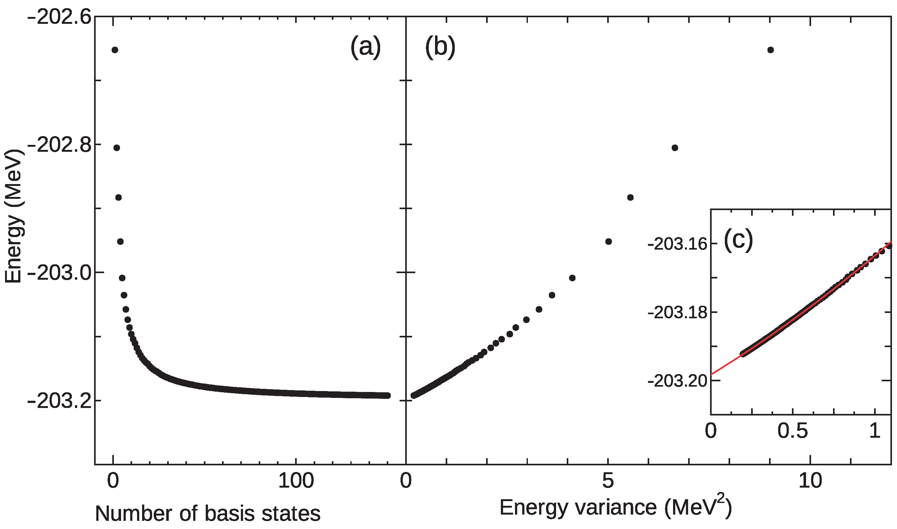
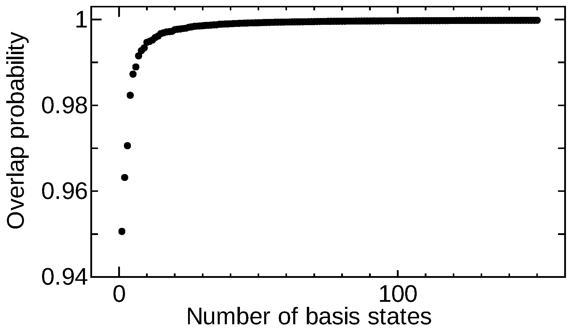
3.2. Quasiparticle Vacua Shell Model

The MCSM wave function is a linear combination of the Slater determinants, which are not suitable for treating the pairing correlation in the heavy-mass region. In order to include the pairing correlation efficiently, one can replace the Slater-determinant basis by the number projected quasi-particle vacua. This framework is called the “QVSM“ [24]. The QVSM wave function is defined as
| Ψ ( N b ) = n = 1 N b K = J J f i K P M K J π P Z P N | ϕ n
where P Z and P N are the proton and neutron number projectors, respectively. | ϕ n is a quasiparticle vaccum and is given as
β k ( n ) | ϕ n = 0 for any k , β k ( n ) = i ( V i k ( n ) * c i + U i k ( n ) * c i ) ,
where β k denotes a quasi-particle annihilation operator and c i is the creation operator of the single-particle orbit i. Thus, the basis state is parametrized by the complex matrices U and V which keep the orthogonalization condition [78]. In the present work, this quasiparticle does not mix the proton and neutron spaces. The energy is obtained in the same manner to the MCSM by solving Equation (9). U ( n ) and V ( n ) matrices are determined utilizing the conjugate gradient method to minimize E ( n ) .
As a benchmark test, shell-model calculations of 132 Ba were performed with the SN100PN interaction [79] and the j j 55 model space. Figure 3 represents the results of various approximation frameworks. In Figure 3, (a)–(d) present the results of the generator coordinate methods (GCM) discussed in [58] in comparison with the MCSM result (e), the QVSM result (f), and the exact shell-model energy (g). Figure 3A shows that the two GCM results with the Slater determinants, (a) and (b), have 2 MeV or a larger deviation from the exact one. The GCM results with the quasiparticle vacua basis, the MCSM result, and the QVSM result show the deviation smaller than 1 MeV. The QVSM is the best result, the deviation of which is only 45 keV.
Figure 3B shows the excitation energies of the yrast band ( 2 1 + , 4 1 + , 6 1 + , and 8 1 + ) and the quasi-gamma band ( 2 2 + , 3 1 + , 4 2 + , 5 1 + , and 6 2 + ) of 132 Ba. The two GCM methods with the Slater determinant basis states, (a) and (b), present too low excitation energies of the yrast band because of the underestimation of the pairing correlation. The two GCM methods with the quasiparticle vacua basis, (c) and (d) show the correct excitation energies of the yrast band. Two GCM methods assuming axial symmetry, (a) and (c), apparently failed to reproduce the quasi-gamma band. The GCM method with the quasiparticle vacua basis is referred to as the HFB+GCM (“HFB” stands for “Hartree-Fock-Bogoliubov”) in Figure 3. The HFB+GCM result shows reasonable agreement with the exact one. The MCSM also shows the reasonable agreement with the exact one, the moment of inertia is slightly overestimated because of the underestimation of the pairing correlation. The QVSM result shows the almost perfect agreement with the exact one.
This benchmark test confirms that the QVSM outperforms the GCM and the MCSM in this mass region. Indeed, the QVSM wave function is superior to the MCSM wave function of the same N b by including the pairing correlation efficiently. However, the computation time of the QVSM is longer than the MCSM with the same N b mainly due to the number projection. If the difference between the MCSM and QVSM energies with the same N b is small, the MCSM can surpass the QVSM by increasing N b within the same computation time. In Ref. [24], we demonstrated that in the case of 68 Ni in the p f g 9 / 2 d 5 / 2 model space the MCSM and QVSM energies have small deviation with the same N b , and thus the MCSM is efficient in terms of the computation time. In practice, one can try both the QVSM and the MCSM with a small N b and identify which one is efficient before performing heavy calculations. Empirically, it was found that the QVSM is more efficient in nuclei heavier than tin isotopes, in which the pairing correlation becomes important.
As another test of the QVSM, one can perform shell-model calculation of 101 Sn with the 0 g 9 / 2 , 0 g 7 / 2 , 1 d 5 / 2 , 1 d 3 / 2 , and 2 s 1 / 2 orbits as the model space. One adopts an effective interaction derived in an ab initio way, the VS-IMSRG method [15,80]. In the derivation, the chiral N 3 LO 1.8/2.0(EM) (see details in Ref. [81]) was adopted for the two-body and three-body forces with a similarity-renormalization-group evolution. Figure 4 shows the results of the 7 / 2 1 + and 5 / 2 1 + energies of 101 Sn provided by ITSM (Figure 4a), the Lanczos diagonalization with particle-hole truncation (Figure 4b), and the QVSM (Figure 4c).
Figure 4a shows the ITSM result as a function of the number of the allowed particle-hole excitation across the N = Z = 50 gap, T max [80]. The result shows good convergence as a function of T max and predicts the ground 7 / 2 + state and the small excitation energy of the 5 / 2 + state. Note that it does not mean a variational upper limit, since these results are extrapolated values as a function of the importance measure. Figure 4b shows the Lanczos diagonalization result with restricting t-particle t-hole excitation across the N = Z = 50 gap. The M-scheme dimension of t = 6 is 9.6 × 10 9 , which is quite large. The energies gradually lower as a function of t, but still it does not reach sufficient convergence. Figure 4c presents the QVSM results against the energy variance. as N b increases the energy and energy variance decreases smoothly and approaches the y-axis or zero energy variance. The y-intercepts of the fitted curve become the extrapolated values, which predict the 7 / 2 + ground state with small 5 / 2 + excitation energy.
Thus, these three methods predict the 7 / 2 + ground state and small excitation energy of the 5 / 2 + state consistently. The extrapolated value of the QVSM seems consistent with the behavior of and the diagonalization result with the t-particle t-hole truncation.

4. Summary

I reviewed the current status of the shell-model calculations, and our developments to overcome the limitation of the conventional Lanczos diagonalization method. One of the frontiers of shell-model study is to study neutron-rich nuclei towards the neutron drip line, in which a larger model space is required. To perform shell-model calculations with such a large model space, the MCSM was proposed and demonstrated in Section 3.1. The MCSM has been applied to various studies of exotic nuclei [23]. Another frontier is to go heavier open-shell nuclei, in which pairing correlation is essential to be treated efficiently. For such purpose, the QVSM has been developed and its feasibility was demonstrated in Section 3.2. Several benchmark tests to demonstrate the capabilities of the MCSM and QVSM methods are presented.
Other frontiers for the shell-model study are the microscopic description of giant resonance and statistical properties of the highly excited region. The Lanczos strength function method [1] is a solution to this problem, but it is still trapped by the rapid growth of the shell-model dimension. Although several attempts were performed to go beyond this limit, which shows promising results [82], further study is required.

Funding

This research was supported by “Program for Promoting Researches on the Supercomputer Fugaku” (JPMXP1020200105) and JICFuS, and KAKENHI grant (17K05433, 20K03981).

Data Availability Statement

The data used in this work are available from the author upon reasonable request.

Acknowledgments

The author acknowledges Takashi Abe, Michio Honma, Takaharu Otsuka, Takayuki Miyagi, Takahiro Mizusaki, Tomoaki Togashi, Yusuke Tsunoda, and Yutaka Utsuno for fruitful collaborations. I especially thank Takayuki Miyagi for providing us with the VS-IMSRG interaction for 101 Sn. This research used computational resources of the supercomputer Fugaku (hp220174, hp210165, hp200130) at the RIKEN Center for Computational Science, Oakforest-PACS supercomputer, Wisteria supercomputer (CCS-Tsukuba MCRP xg18i035 and wo22i022) and Oakbridge-CX supercomputer.

Conflicts of Interest

The author declares no conflict of interest.

References

  1. Caurier, E.; Martinez-Pinedo, G.; Nowacki, F.; Poves, A.; Zuker, A.P. The shell model as unified view of nuclear structure. Rev. Mod. Phys. 2005, 77, 427–488. [Google Scholar] [CrossRef]
  2. Otsuka, T.; Gade, A.; Sorlin, O.; Suzuki, T.; Utsuno, Y. Evolution of shell structure in exotic nuclei. Rev. Mod. Phys. 2020, 92, 015002. [Google Scholar] [CrossRef]
  3. Martínez-Pinedo, G.; Langanke, K. Shell model applications in nuclear astrophysics. Physics 2022, 4, 677–689. [Google Scholar] [CrossRef]
  4. Shimizu, N.; Togashi, T.; Utsuno, Y. Gamow-Teller transitions of neutron-rich N=82, 81 nuclei by shell-model calculations. Prog. Theor. Exp. Phys. 2021, 2021, 033D01. [Google Scholar] [CrossRef]
  5. Menéndez, J.; Poves, A.; Caurier, E.; Nowacki, F. Disassembling the nuclear matrix elements of the neutrinoless ββ decay. Nucl. Phys. A 2009, 818, 139–151. [Google Scholar] [CrossRef]
  6. Coraggio, L.; Gargano, A.; Itaco, N.; Mancino, R.; Nowacki, F. Calculation of the neutrinoless double-β decay matrix element within the realistic shell model. Phys. Rev. C 2020, 101, 044315. [Google Scholar] [CrossRef]
  7. Shimizu, N.; Menéndez, J.; Yako, K. Double Gamow-Teller transitions and its relation to neutrinoless ββ decay. Phys. Rev. Lett. 2018, 120, 142502. [Google Scholar] [CrossRef]
  8. Yanase, K.; Shimizu, N. Large-scale shell-model calculations of nuclear Schiff moments of 129Xe and 199Hg. Phys. Rev. C 2020, 102, 065502. [Google Scholar] [CrossRef]
  9. Cohen, S.; Kurath, D. Effective interactions for the 1p shell. Nucl. Phys. 1965, 73, 1–24. [Google Scholar] [CrossRef]
  10. Brown, B.A.; Richter, W. New “USD” Hamiltonians for the sd shell. Phys. Rev. C 2006, 74, 034315. [Google Scholar] [CrossRef] [Green Version]
  11. Honma, M.; Otsuka, T.; Brown, B.A.; Mizusaki, T. New effective interaction for pf shell nuclei and its implications for the stability of the N=Z=28 closed core. Phys. Rev. C 2004, 69, 034335. [Google Scholar] [CrossRef]
  12. Richter, W.A.; Van Der Merwe, M.G.; Julies, R.E.; Brown, B.A. New effective interactions for the 0f1p shell. Nucl. Phys. A 1991, 523, 325–353. [Google Scholar] [CrossRef]
  13. Honma, M.; Otsuka, T.; Mizusaki, T.; Hjorth-Jensen, M. New effective interaction for f5pg9-shell nuclei. Phys. Rev. C 2009, 80, 064323. [Google Scholar] [CrossRef]
  14. Hjorth-Jensen, M.; Kuo, T.T.S.; Osnes, E. Realistic effective interactions for nuclear systems. Phys. Rep. 1995, 261, 125–270. [Google Scholar] [CrossRef]
  15. Stroberg, S.R.; Henderson, J.; Hackman, G.; Ruotsalainen, P.; Hagen, G.; Holt, J.D. Systematics of E2 strength in the sd shell with the valence-space in-medium similarity renormalization group. Phys. Rev. C 2022, 105, 034333. [Google Scholar] [CrossRef]
  16. Jansen, G.R.; Engel, J.; Hagen, G.; Navratil, P.; Signoracci, A. Ab-initio coupled-cluster effective interactions for the shell model: Application to neutron-rich oxygen and carbon isotopes. Phys. Rev. Lett. 2014, 113, 142502. [Google Scholar] [CrossRef] [PubMed]
  17. Coraggio, L.; De Gregorio, G.; Gargano, A.; Itaco, N.; Fukui, T.; Ma, Y.Z.; Xu, F.R. Shell-model study of calcium isotopes toward their drip line. Phys. Rev. C 2020, 102, 054326. [Google Scholar] [CrossRef]
  18. Tsunoda, N.; Otsuka, T.; Shimizu, N.; Hjorth-Jensen, M.; Takayanagi, K.; Suzuki, T. Exotic neutron-rich medium-mass nuclei with realistic nuclear forces. Phys. Rev. C 2017, 95, 021304. [Google Scholar] [CrossRef]
  19. Smirnova, N.A.; Barrett, B.R.; Kim, Y.; Shin, I.J.; Shirokov, A.M.; Dikmen, E.; Maris, P.; Vary, J.P. Effective interactions in the sd shell. Phys. Rev. C 2019, 100, 054329. [Google Scholar] [CrossRef]
  20. Miyagi, T.; Stroberg, S.R.; Holt, J.D.; Shimizu, N. Ab initio multishell valence-space Hamiltonians and the island of inversion. Phys. Rev. C 2020, 102, 034320. [Google Scholar] [CrossRef]
  21. Tsunoda, N.; Otsuka, T.; Takayanagi, K.; Shimizu, N.; Suzuki, T.; Utsuno, Y.; Yoshida, S.; Ueno, H. The impact of nuclear shape on the emergence of the neutron dripline. Nature 2020, 587, 66–71. [Google Scholar] [CrossRef] [PubMed]
  22. Otsuka, T.; Honma, M.; Mizusaki, T.; Shimizu, N.; Utsuno, Y. Monte Carlo shell model for atomic nuclei. Prog. Part. Nucl. Phys. 2001, 47, 319–400. [Google Scholar] [CrossRef]
  23. Shimizu, N.; Abe, T.; Honma, M.; Otsuka, T.; Togashi, T.; Tsunoda, Y.; Utsuno, Y.; Yoshida, T. Monte Carlo shell model studies with massively parallel supercomputers. Phys. Scr. 2017, 92, 063001. [Google Scholar] [CrossRef]
  24. Shimizu, N.; Tsunoda, Y.; Utsuno, Y.; Otsuka, T. Variational approach with the superposition of the symmetry-restored quasiparticle vacua for nuclear shell-model calculations. Phys. Rev. C 2021, 103, 014312. [Google Scholar] [CrossRef]
  25. Brown, B.A.; Etchegoyen, A.; Rae, W.D.M.; Godwin, N.S. The Computer Code OXBASH; MSU-NSCL Report 524; National Superconducting Cyclotron Laboratory: East Lansing, MI, USA, 1988. [Google Scholar]
  26. Brown, B.A.; Etchegoyen, A.; Godwin, N.S.; Rae, W.D.M.; Richter, W.A.; Ormand, W.E.; Warburton, E.K.; Winfield, J.S.; Zhao, L.; Zimmerman, C.H. Oxbash for Windows PC; MSU-NSCL Report 1289; National Superconducting Cyclotron Laboratory: East Lansing, MI, USA, 2004. [Google Scholar]
  27. Brown, B.A.; Rae, W.D.M. The shell-model code NuShellX@ MSU. Nucl. Data Sheets 2014, 120, 115–118. [Google Scholar] [CrossRef]
  28. Caurier, E. Computer Code ANTOINE; Centre de Recherches Nucléaires: Strasbourg, France, 1989. [Google Scholar]
  29. Caurier, E.; Nowacki, F. Coupled Code NATHAN; Centre de Recherches Nucléaires: Strasbourg, France, 1995. [Google Scholar]
  30. Mizusaki, T. Development of a new code for large-scale shell-model calculations using a parallel computer. RIKEN Accel. Prog. Rep. 1999, 33, 14. Available online: https://www.nishina.riken.jp/researcher/APR/Document/ProgressReport_vol_33.pdf (accessed on 24 August 2020).
  31. Mizusaki, T.; Shimizu, N.; Utsuno, Y.; Honma, M. The MSHELL64 code. 2013; unpublished. [Google Scholar]
  32. Shao, M.; Aktulga, H.M.; Yang, C.; Ng, E.G.; Maris, P.; Vary, J.P. Accelerating nuclear configuration interaction calculations through a preconditioned block iterative eigensolver. Comput. Phys. Commun. 2018, 222, 1–13. [Google Scholar] [CrossRef]
  33. Johnson, C.W.; Ormand, W.E.; Krastev, P.G. Factorization in large-scale many-body calculations. Comput. Phys. Commun. 2013, 184, 2761–2774. [Google Scholar] [CrossRef]
  34. Shimizu, N.; Mizusaki, T.; Utsuno, Y.; Tsunoda, Y. Thick-restart block Lanczos method for large-scale shell-model calculations. Comput. Phys. Commun. 2019, 244, 372–384. [Google Scholar] [CrossRef]
  35. Lanczos, C. An iteration method for the solution of the eigenvalue problem of linear differential and integral operators. J. Res. Nat. Bur. Standards 1950, 45, 255–282. [Google Scholar] [CrossRef]
  36. Shimizu, N.; Utsuno, Y.; Futamura, Y.; Sakurai, T.; Mizusaki, T.; Otsuka, T. Stochastic estimation of level density in nuclear shell-model calculations. EPJ Web Conf. 2016, 122, 02003. [Google Scholar] [CrossRef] [Green Version]
  37. Wu, K.; Simon, H. Thick-restart Lanczos method for large symmetric eigenvalue problems. SIAM J. Matrix Anal. Appl. 2000, 22, 602–616. [Google Scholar] [CrossRef]
  38. Aktulga, H.M.; Afibuzzaman, M.; Williams, S.; Buluç, A.; Shao, M.; Yang, C.; Ng, E.G.; Maris, P.; Vary, J.P. A high performance block eigensolver for nuclear configuration interaction calculations. IEEE Trans. Parallel Distrib. Syst. 2017, 28, 1550–1563. [Google Scholar] [CrossRef]
  39. Mizusaki, T.; Kaneko, K.; Honma, M.; Sakurai, T. Filter diagonalization of shell-model calculations. Phys. Rev. C 2010, 82, 024310. [Google Scholar] [CrossRef]
  40. Ikegami, T.; Sakurai, T.; Nagashima, U. A filter diagonalization for generalized eigenvalue problems based on the Sakurai—Sugiura projection method. J. Comput. Appl. Math 2010, 233, 1927–1936. [Google Scholar] [CrossRef]
  41. Shimizu, N.; Utsuno, Y.; Futamura, Y.; Sakurai, T.; Mizusaki, T.; Otsuka, T. Stochastic estimation of nuclear level density in the nuclear shell model: An application to parity-dependent level density in 58Ni. Phys. Lett. B 2016, 753, 13–17. [Google Scholar] [CrossRef]
  42. Michel, N.; Aktulga, H.M.; Jaganathen, Y. Toward scalable many-body calculations for nuclear open quantum systems using the Gamow Shell Model. Comput. Phys. Commun. 2020, 247, 106978. [Google Scholar] [CrossRef]
  43. Mizusaki, T.; Myo, T.; Katō, K. A new approach for many-body resonance spectroscopy with the complex scaling method. Prog. Theor. Exp. Phys. 2014, 2014, 091D01. [Google Scholar] [CrossRef]
  44. Koonin, S.E.; Dean, D.J.; Langanke, K. Shell model Monte Carlo methods. Phys. Rep. 1997, 278, 1–77. [Google Scholar] [CrossRef]
  45. Adami, C.; Koonin, S.E. Complex Langevin equation and the many fermion problem. Phys. Rev. C 2001, 63, 034319. [Google Scholar] [CrossRef]
  46. Bonnard, J.; Juillet, O. Constrained-path quantum Monte Carlo approach for the nuclear shell model. Phys. Rev. Lett. 2013, 111, 012502. [Google Scholar] [CrossRef] [PubMed] [Green Version]
  47. Alhassid, Y.; Bonett-Matiz, M.; Liu, S.; Nakada, H. Direct microscopic calculation of nuclear level densities in the shell model Monte Carlo approach. Phys. Rev. C 2015, 92, 024307. [Google Scholar] [CrossRef]
  48. Dukelsky, J.; Pittel, S.; Dimitrova, S.; Stoitsov, M. Density matrix renormalization group method and large-scale nuclear shell-model calculations. Phys. Rev. C 2002, 65, 054319. [Google Scholar] [CrossRef]
  49. Pittel, S.; Sandulescu, N. Density matrix renormalization group and the nuclear shell model. Phys. Rev. C 2006, 73, 014301. [Google Scholar] [CrossRef]
  50. Legeza, Ö.; Veis, L.; Poves, A.; Dukelsky, J. Advanced density matrix renormalization group method for nuclear structure calculations. Phys. Rev. C 2015, 92, 051303. [Google Scholar] [CrossRef]
  51. Hara, K.; Sun, Y. Projected shell model and high-spin spectroscopy. Int. J. Mod. Phys. E 1995, 4, 637–785. [Google Scholar] [CrossRef]
  52. Gao, Z.-C.; Horoi, M. Angular momentum projected configuration interaction with realistic Hamiltonians. Phys. Rev. C 2009, 79, 014311. [Google Scholar] [CrossRef]
  53. Jiao, L.F.; Sun, Z.H.; Xu, Z.X.; Xu, F.R.; Qi, C. Correlated-basis method for shell-model calculations. Phys. Rev. C 2014, 90, 024306. [Google Scholar] [CrossRef]
  54. Mizusaki, T.; Shimizu, N. New variational Monte Carlo method with an energy variance extrapolation for large-scale shell-model calculations. Phys. Rev. C 2012, 85, 021301. [Google Scholar] [CrossRef]
  55. Shimizu, N.; Mizusaki, T. Variational Monte Carlo method for shell-model calculations in odd-mass nuclei and restoration of symmetry. Phys. Rev. C 2018, 98, 054309. [Google Scholar] [CrossRef]
  56. Yoshinaga, N.; Higashiyama, K. Systematic studies of nuclei around mass 130 in the pair-truncated shell model. Phys. Rev. C 2004, 69, 054309. [Google Scholar] [CrossRef]
  57. Zhao, Y.M.; Arima, A. Nucleon-pair approximation to the nuclear shell model. Phys. Rep. 2014, 545, 1–45. [Google Scholar] [CrossRef]
  58. Shimizu, N.; Mizusaki, T.; Kaneko, K.; Tsunoda, Y. Generator-coordinate methods with symmetry-restored Hartree-Fock-Bogoliubov wave functions for large-scale shell-model calculations. Phys. Rev. C 2021, 103, 064302. [Google Scholar] [CrossRef]
  59. Schmid, K.W. On the use of general symmetry-projected Hartree–Fock–Bogoliubov configurations in variational approaches to the nuclear many-body problem. Prog. Part. Nucl. Phys. 2004, 52, 565–633. [Google Scholar] [CrossRef]
  60. Schmid, K.W.; Grümmer, F.; Kyotoku, M.; Faessler, A. Selfconsistent description of non-yrast states in nuclei: The excited VAMPIR approach. Nucl. Phys. A 1986, 452, 493–512. [Google Scholar] [CrossRef]
  61. Puddu, G. Hybrid schemes for the calculation of low-energy levels of shell model Hamiltonians. J. Phys. G Nucl. Part. Phys. 2006, 32, 321–331. [Google Scholar] [CrossRef]
  62. Puddu, G. Calculation of energy levels with the hybrid multi-determinant method in the fp region. Eur. Phys. J. A 2007, 34, 413–415. [Google Scholar] [CrossRef]
  63. Puddu, G. A study of open shell nuclei using chiral two-body interactions. J. Phys. G Nucl. Part. Phys. 2021, 48, 045105. [Google Scholar] [CrossRef]
  64. Horoi, M.; Brown, B.A.; Zelevinsky, V. Exponential convergence method: Nonyrast states, occupation numbers, and a shell-model description of the superdeformed band in 56Ni. Phys. Rev. C 2003, 67, 034303. [Google Scholar] [CrossRef]
  65. Mizusaki, T.; Imada, M. Extrapolation method for shell model calculations. Phys. Rev. C 2002, 65, 064319. [Google Scholar] [CrossRef]
  66. Zhan, H.; Nogga, A.; Barrett, B.R.; Vary, J.P.; Navratil, P. Extrapolation method for the no-core shell model. Phys. Rev. C 2004, 69, 034302. [Google Scholar] [CrossRef] [Green Version]
  67. Shimizu, N.; Utsuno, Y.; Mizusaki, T.; Otsuka, T.; Abe, T.; Honma, M. Novel extrapolation method in the Monte Carlo shell model. Phys. Rev. C 2010, 82, 061305. [Google Scholar] [CrossRef]
  68. Puddu, G. An efficient method to evaluate energy variances for extrapolation methods. J. Phys. G Nucl. Part. Phys. 2012, 39, 085108. [Google Scholar] [CrossRef]
  69. Stumpf, C.; Braun, J.; Roth, R. Importance-truncated large-scale shell model. Phys. Rev. C 2016, 93, 021301(R). [Google Scholar] [CrossRef]
  70. Roth, R.; Navrátil, P. Ab initio study of 40Ca with an importance-truncated no-core shell model. Phys. Rev. Lett. 2007, 99, 092501. [Google Scholar] [CrossRef]
  71. Honma, M.; Mizusaki, T.; Otsuka, T. Diagonalization of Hamiltonians for many-body systems by auxiliary field quantum Monte Carlo technique. Phys Rev. Lett. 1995, 75, 1284–1287. [Google Scholar] [CrossRef]
  72. Honma, M.; Mizusaki, T.; Otsuka, T. Nuclear shell model by the quantum Monte Carlo diagonalization method. Phys Rev. Lett. 1996, 77, 3315–3318. [Google Scholar] [CrossRef]
  73. Shimizu, N.; Abe, T.; Tsunoda, Y.; Utsuno, Y.; Yoshida, T.; Mizusaki, T.; Honma, M.; Otsuka, T. New-generation Monte Carlo shell model for the K computer era. Prog. Theor. Exp. Phys. 2012, 2012, 01A205. [Google Scholar] [CrossRef]
  74. Shimizu, N.; Tsunoda, Y. SO(3) quadratures in angular-momentum projection. arXiv 2022, arXiv:2205.04119. [Google Scholar]
  75. Utsuno, Y.; Shimizu, N.; Otsuka, T.; Abe, T. Efficient computation of Hamiltonian matrix elements between non-orthogonal Slater determinants. Comput. Phys. Commun. 2013, 184, 102–108. [Google Scholar] [CrossRef]
  76. Horoi, M.; Brown, B.A.; Otsuka, T.; Honma, M.; Mizusaki, T. Shell model analysis of the 56Ni spectrum in the full pf model space. Phys. Rev. C 2006, 73, 061305(R). [Google Scholar] [CrossRef]
  77. Otsuka, T.; Honma, M.; Mizusaki, T. Structure of the N=Z=28 closed shell studied by Monte Carlo shell model calculation. Phys. Rev. Lett. 1998, 81, 1588–1591. [Google Scholar] [CrossRef]
  78. Ring, P.; Schuck, P. The Nuclear Many-Body Problem; Springer: Berlin/Heidelberg, Germany, 2004. [Google Scholar]
  79. Brown, B.A.; Stone, N.J.; Stone, J.R.; Towner, I.S.; Hjorth-Jensen, M. Magnetic moments of the 2 1 + states around 132Sn. Phys. Rev. C 2005, 71, 044317. [Google Scholar] [CrossRef]
  80. Morris, T.D.; Simonis, J.; Stroberg, S.R.; Stumpf, C.; Hagen, G.; Holt, J.D.; Jansen, G.R.; Papenbrock, T.; Roth, R.; Schwenk, A. Structure of the lightest tin isotopes. Phys. Rev. Lett. 2018, 120, 152503. [Google Scholar] [CrossRef] [PubMed]
  81. Hebeler, K.; Bogner, S.; Furnstahl, R.J.; Nogga, A.; Schwenk, A. Improved nuclear matter calculations from chiral low-momentum interactions. Phys. Rev. C 2011, 83, 031301(R). [Google Scholar] [CrossRef]
  82. Togashi, T.; Otsuka, T.; Shimizu, N.; Utsuno, Y. E1 strength function in the Monte Carlo shell model. JPS Conf. Proc. 2018, 23, 012031. [Google Scholar] [CrossRef]
Figure 1. MCSM results of 56 Ni with the FPD6 interaction. (a): MCSM energy against the number of the MCSM basis states. (b): extrapolation plot with the energy variance. (c): magnified view of (b). The red is the fitted curve with a second-order polynomial. See text for details.
Physics 04 00071 g001
Figure 2. Overlap probability between the MCSM wave function and the exact wave function by the Lanczos method against the number of the MCSM basis states N b . These wave functions were computed for the ground state of 56 Ni with the FPD6 interaction [12].
Physics 04 00071 g002
Figure 3. Shell-model results of 132 Ba with the SN100PN interaction by various approximation methods. (A): the difference of shell-model energies from the exact one. (B): the excitation energies of the ground-state band ( 2 1 + , 4 1 + , 6 1 + and 8 1 + ) and the quasi- γ band ( 2 2 + , 3 1 + , 4 2 + , 5 1 + , and 6 2 + ). The results are shown for: (a) generator-coordinate method (GCM) with the Hartree-Fock (HF) calculations assuming axial symmetry, (b) GCM with the HF calculations without assuming axial symmetry, (c) GCM with the Hartree-Fock-Bogoliubov (HFB) calculations assuming axial symmetry, (d) GCM with the HFB calculations without assuming axial symmetry, (e) MCSM with 50 basis states without variance extrapolation, (f) QVSM with 30 basis states without variance extrapolation, and (g) exact shell-model result by the Lanczos diagonalization. Numerical data of (a–d) and (g) are taken from Ref. [58].
Physics 04 00071 g003
Figure 4. Energies of the 5 / 2 + (red) and 7 / 2 + (black) states of 101 Sn. (a): ITSM result against T max from Ref. [80]. (b): Result of the Lanczos diagonalization with t-particle t-hole truncation. (c): QVSM with 60 basis states. The solid lines in (c) are fitted for the extrapolation. See text for details.
Physics 04 00071 g004
Table 1. M-scheme and J-scheme dimensions of several nuclei. The dimension of the M π = 0 + ( J π = 0 + ) subspace is shown. See text for details.
NuclideModel SpaceM-Scheme DimJ-Scheme Dim
12 C 2 N , Z 8 (p shell)519
28 Si 8 N , Z 20 ( s d shell)93,7103372
56 Ni 20 N , Z 40 ( p f shell) 1.08 × 10 9 1.54 × 10 7
78 Y 28 N , Z 50 ( f 5 p g 9 , j j 44 ) 1.31 × 10 10 1.11 × 10 8
130 Sm 50 Z , N 82 ( j j 55 ) 2.06 × 10 15 9.58 × 10 12
172 Dy 50 Z 82 , 82 N 126 1.71 × 10 19 5.54 × 10 16
( j j 56 )
Publisher’s Note: MDPI stays neutral with regard to jurisdictional claims in published maps and institutional affiliations.

