2. Nuclei with Closed Shells: An Experimental Perspective
Nuclei with closed shells, both singly and doubly closed, have been the base upon which the shell model has been built. However, such nuclei are neither manifestations of nor a sound basis for the shell model in its extreme independent-particle form. Such nuclei (i.e., closed shell) can usefully be classified into three types: doubly closed shell nuclei with equal numbers of protons (Z) and neutrons (N), i.e., ; doubly closed shell nuclei with ; and singly closed shell nuclei.
The distinction of doubly closed shell nuclei with
is that they exhibit shape coexistence at low energy, even at the level of the first excited states in
O and
Ca, as shown in
Figure 1. In doubly even nuclei with
, shown in
Figure 2, shape coexistence has not yet been observed. The simple explanation is that, for
, spatial overlap of the proton and neutron configurations is maximal, and it is proton–neutron correlations that are deformation producing.
The distinction of singly closed shell nuclei is that they are dominated by the emergence of pairing correlations. Pairing correlations are concisely formulated using the concept of the seniority quantum number,
v, i.e., the number of unpaired nucleons. This was first recognized by Maria Goeppert-Mayer [
9,
10]. The quantum mechanics of pairing correlations is concisely, even elegantly, described using quasispin, as introduced by Arthur Kerman [
11]. The basic features of quasispin, as applied to a series of
configurations, where
n denotes the occupation of the orbit, are shown in
Figure 3; a view which complements that in
Figure 3 is shown for a series of
configurations in
Figure 4. The quasispin algebra is developed in detail in Chapter 6 of [
6]. That Chapter includes a thorough treatment of the origins of the key ideas from Racah’s seniority [
12,
13,
14] through Flowers’ handling of
coupling [
15], Helmers’ unitary symplectic invariants [
16], Lawson and Macfarlane’s identification of the rank-1/2 quasispin
su(2) tensorial character of one-body annihilation and creation operators [
17], to Kerman’s simple formulation [
11]. Furthermore, it can be noted that there is a profound duality structure residing in these algebras [
18], which shows how algebraic structure provides insight into the complexity of many-body quantum systems. A pedagogical treatment of the quasispin algebra is presented in Chapter 4 in [
5]. That Chapter illustrates how P.W. Anderson’s idea [
19] provided the first conceptual recognition of quasispin as the essential algebraic structure underlying many-fermion systems with Cooper pairs [
20].
Experimentally, the seniority coupling scheme is realized essentially exactly when the low-energy structure of singly closed shell nuclei is dominated by a high-
j orbital. This is shown in
Figure 5 for
neutron subshell filling in the Sn isotopes and in
Figure 6 for
proton subshell filling in the
isotones. The patterns are almost indistinguishable. The domination of seniority extends into patterns of electric quadrupole,
transition probabilities: this is shown in
Figure 7 for
configurations in even-Cd and even-Pd nuclei with
and
. The pattern of
matrix elements in nuclei dominated by seniority coupling shows a smoothly changing character which is well described by the following relationship for the reduced transition strength [
6]:
where
and
are spins of initial and final states,
s,
are quasispin quantum numbers, details of which appear in
Figure 3;
is an
su(2) Clebsch–Gordan coefficient and
, e.g.,
for
. This Clebsch–Gordan coefficient emerges from the quasispin
su(2) algebra when applying the Wigner–Eckart theorem to the
operator: this operator is a rank-1 quasispin tensor. Details are beyond the present discussion and are given in [
6]. (Note:
(designated by the Greek letter nu) is distinct from the seniority quantum number,
v (designated by the Latin letter vee).) This relationship is illustrated in
Figure 8 and
Figure 9 for the
configurations in the even-mass Sn isotopes and
isotones, respectively. Indeed, these patterns are one of the best signatures of structure unique to singly closed shell nuclei. However, the clarity and interpretation of these structures are dictated by quantum mechanics that is beyond that of the independent-particle shell model in that correlations in the form of Cooper pairs have emerged. Pairing Hamiltonians can be derived as a simplification of the nucleon–nucleon residual interaction; however, the focus here is on the empirical simplicity of the seniority structures that persist toward mid-shell where the number of valence nucleons is large, in contrast with the connection between pairing correlations and the two-body residual interactions in a large-basis shell model calculation, which is not obvious. Stated in rhetorical terms: Could one ascertain the algebraic structure of Cooper pairs, in the guise of quasispin, and manifestly controlling structure in all singly closed shell nuclei, based on a shell model computational program? Once the quasispin structure is recognized, its implications for the residual interactions required in the shell model can be explored so that the structure emerges from the calculations.
In the remainder of this Section, some observations are made with respect to the mathematical structure on which quasispin is based, in order to place this shell model view into perspective.
The arrival at the concept of quasispin as a degree of freedom in nuclei requires the recognition of mathematical structures that are not obvious. A brief sketch of the essential details is given here in words. Full details are given by Rowe and Wood [
6] and, at an introductory level, by Heyde and Wood [
5]. Specifically, the quasispin algebra is recognized by expressing the Hamiltonian and the interaction using second quantization. The mathematics emerge by taking bilinear combinations of the elements (one-body fermionic creation and annihilation operators) of a Jordan algebra (anticommutator brackets of the creation and annihilation operators). These bilinear combinations obey a Lie algebra (commutator brackets). This is impossible to see until one works out the Lie bracket values of the bilinear combinations, which is done by expanding them using anticommutator bracket relations so as to express everything in terms of Jordan algebra elements in “normal order”; see Equation (4.93) in Ref. [
5]. Normal order means annihilation operators all to the right and creation operators all to the left. Furthermore, the Lie bracket algebra for a Jordan algebra element (single creation or annihilation operator) with quasispin algebra elements (bilinear combinations of creation and annihilation operators) reveals that the creation and annihilation operators are rank-1/2 quasispin tensors. This is also impossible to see until one works out the Lie bracket values. Indeed, rank-1/2 tensors are unknown in spin-angular momentum theory; see p. 423 in Ref. [
6] for additional details.
Spectroscopy of low-spin and medium-spin states is beginning to provide a comprehensive (near-complete) view of excited states in doubly even nuclei at and near closed shells. Consequently, seniority coupling has been shown to apply in nuclei where the structure is dominated by two medium-spin
j shells. This is illustrated in
Figure 10 and
Figure 11 for the
isotones with
. The
structures in
Te,
Xe,
Ba, and
Ce are labelled in
Figure 10: these include the
structures, with
, 4, and 6, and the
-
structures, with
, 2, 3, 4, 5, and 6. In
Xe only, as expected,
structures are observed with the allowed spins,
, 4, 5, and 8, cf.
Figure 3. The comprehensive view of
Xe is the result of an
study [
30]. Note that this seniority-based organization of data is essentially complete; for example, there is no excited
state observed, as might be expected from a
coupling—such a coupling is forbidden by the Pauli exclusion principle if the
states are seniority-dominated structures. The
values and the magnetic moments,
, are shown for reference and discussed further in
Figure 12 as the
g factors, where
.
The seniority structure of the
isotones and its breakdown is an issue for future detailed study. However, shell model calculations affirm the dominant seniority structures. The case of
Xe has been studied comprehensively [
30,
32].
Table 1 shows experimental
values between low-excitation states in
Xe in comparison to the
seniority model, as well as several shell model calculations that include all orbits in the
major shell but use alternative interactions. The
data indeed demonstrate the pattern predicted by the seniority scheme. It should be noted that
Xe represents the mid-shell for the
orbit, for which several
transitions are forbidden. In such cases, the observed transition strengths result from small components of the wavefunction, which can lead to considerable variations in the shell model predictions, despite the calculations agreeing on the dominant structure of the states. It was noted in [
32] that the large-basis shell model calculations support the dominant configurations assigned in the
seniority model up to the
state at 2.1 MeV excitation, although there is considerable configuration mixing. The
model accounts for all states up to about 2.8 MeV, with the exception of the 0
state (more on the 0
state below in this Section). However, above the 2.1-MeV
state, where the level of density increases, the correspondence between the two-level and full basis is less clear.
The
states are consistent with a multi-pair structure distributed over the
and
orbitals. For example, the
jj55 model with
sn100 interactions [
33] has dominant configurations of
(76%) [
Te],
(45%) [
Xe], and
(51%) [
Ba], for the 0
states.
Figure 12 shows the experimental
g factors of the 2
states and the
values of the even-even
isotones with
, and compares them with large-basis shell model calculations. In addition, the ground-state
g factors of the interleaving odd-
A isotones are shown, which indicate that the Fermi surface moves from the
orbit into the
orbit at
. The
trend is quite well described, but the
trend is not well described, particularly when the Fermi surface moves into the
orbit. In contrast, the odd-
A isotopes are well described. Focusing on the range
, the
g factor data in
Figure 12, for both odd and even-
A isotones, are near constant and thus consistent with a simple
structure in both the ground states (odd-
Z) and 2
states (even-
Z). The lowered experimental
values for
Ce,
Nd and
Sm have been attributed to increasing contributions from
excitations [
36]. Nevertheless, the basic seniority structure appears to persist in these nuclei.
The complete pattern of excitations in odd-mass, singly closed shell nuclei is somewhat more complex than for even-mass singly closed shell nuclei. This is shown for
in the tin isotopes in
Figure 13. Note that the states expected for seniority
range over 14 spin values for
, viz.
3, 5, 7, 9, 9, 11, 13, 15, 15, 17, 19, 21, 23, and 27 (see, e.g., [
37]). The experimental view is incomplete, but there is sufficient detail to conclude that the seniority scheme provides a reliable basis for understanding the low-energy excitations in these isotopes. This perspective is supported by a more global view of odd-mass nuclei shown in
Figure 14, wherein patterns for seniority-three multiplets in selected nuclides and selected spin couplings are visible for
, 9/2, and 11/2. This global behavior appears not to have been recognized. We conjecture that there may be a geometric interpretation of this pattern, similar to the geometrical interpretation of two-body interactions for a pair of identical nucleons in a moderate to high
j orbit, as introduced by Schiffer and True [
38]. An angle between the two spins can be defined, which gives a measure of the overlap of the two orbits for different resultant spins; see discussions in Refs. [
3,
8].
One can conclude that seniority likely provides a complete description of the lowest-energy excited states in singly closed shell nuclei—with one proviso: singly closed shell nuclei exhibit low-energy deformed structures that “coexist” with the low-excitation seniority-dominated structures.
The manifestation of shape coexistence in singly closed shell nuclei was recognized already forty years ago [
39] and was reviewed thirty years ago [
40]. It is well established for
, 50, and 82 and for
and 28; there are hints to its presence for
and 28, and for
, 50, and 82. Details can be found in the most recent review [
41], together with some details in the earlier review [
40]. The emerging view is that shape coexistence likely occurs in all nuclei; including that spherical states occur in nuclei with deformed ground states [
42]. A concise perspective of the occurrence of deformation in nuclei as compared to atoms can be encapsulated in: “The difference between atoms and nuclei is that atoms are a manifestation of many-fermion quantum mechanics with one type of fermion, which repel, whereas nuclei involve two types of nucleon, which attract. By deforming, the system can lower its energy via relaxing the constraints of the Pauli exclusion principle in such a manner that more spatially symmetric configurations become accessible, which leads to a lowering of the energy of the system”. (It can be noted that the emerging view of baryons may signal correlated, even deformed structures, especially the recent realization [
43] that the proton contains more (virtual) anti-down quarks than anti-up quarks: this is simply a manifestation of correlations that involve “particle–hole” excitations, i.e., quark–antiquark pairs, and the Pauli principle.)
3. Hints of Correlations, beyond Pairing and Seniority, at Closed Shells
The dominance of seniority, with intruding shape coexistence, in singly closed shell nuclei is not quite “the whole story”. The following analysis of effective charges implied by the observed in even-even nuclei adjacent to doubly closed shells demonstrates what can be encapsulated in the term “the effective charge problem”.
Electric multipole transition rates in the shell model are usually evaluated using harmonic oscillator wavefunctions. For a single-particle transition
, the reduced matrix element
can be evaluated from
where
and
is the dimensionless radial integral that can be evaluated in closed form with harmonic oscillator wavefunctions. The oscillator length
b is defined as
where
ℏ is the reduced Planck constant,
is the nucleon mass, and
can be evaluated as a function of the mass number
A as
which has been found to give satisfactory agreement with observed charge radii. In general,
For transitions between the states of the pure
configuration, the
values are related to the single-particle matrix element
, by
It is instructive to begin with the textbook cases of O and O, which can be considered as adding one and two neutrons, respectively, to a O core. Identifying the first-excited state to ground, , transition in O as due to the neutron transition from the to orbits, the experimental value of W.u. (Weisskopf units) requires an effective neutron charge of . This value is close to , which is the default often adopted for shell model calculations. However, turning to O, and identifying the transition with , requires to explain the observed transition strength of 3.32(9) W.u. One might hope that this discrepancy between O and O would be resolved by a shell model calculation in the full sd model space with one of the “universal” sd interactions, but it is not. Such shell model calculations describe O well. The same calculations, however, fall short of explaining the in O by a factor of nearly 3. It is worth noting that the experimental for O is based on about 20 independent measurements by four independent techniques, all in reasonable agreement. The conclusion must be that the effective charge handles O, but fails for O due to additional correlations.
Table 2 shows shell model calculations for the reduced transition rate,
, in doubly magic nuclides plus or minus two like nucleons. The shell model calculations were performed with
NuShellX [
44] and generally use a contemporary set of interactions for the relevant basis space, and either the recommended effective charges for the selected basis space, or the default
and
, for protons and neutrons, respectively. The effective charges required to bring the shell model calculations into agreement with experiment are shown. For those nuclides adjacent to
Ca and
Ni, calculations were run in a basis that treats these nuclei as doubly magic, as well as in the full
fp shell, which allows for excitations from the
shell across the
shell gap into the
,
, and
orbits. These calculations account for the neutron core excitation in
Ca, including the
0
state at 5.46 MeV, but cannot describe the
0
state at 4.28 MeV; see
Figure 2, and cf. Figure 60.
There is no overall pattern in the effective charges shown in
Table 2. Most of the shell model
values are within a factor of 2 to 3 of the experiment; however, those for the calcium isotopes,
Ca and
Ca, are underestimated by an order of magnitude. The experimental
value for
Ar is almost a factor of two smaller than theory. While a lifetime measurement [
59] gave a
value consistent with theory, the weight of evidence from independent Coulomb excitation measurements [
45,
60,
61] makes the adopted value in
Table 2 firm and in tension with theory.
Good agreement in the fp-shell calculation is obtained for Ca and Fe. As noted above, in these cases, Ca and Ni are not doubly magic cores but part of the fp model space. It is puzzling that the calculation for Ti in the same model space is twice the experiment, but the restricted model space agrees with experiment.
Moving to heavier nuclei, the effective charges in the
Sn region are near the default values [
62], although most recent calculations adopt
and
[
32,
34,
63,
64]. The measured
for
Sn [
46,
47] is lower than theory and the experimental systematics (see [
65]); the experiment should be repeated.
In the
Pb region,
approaches
. The experimental result for
Po is problematic. As shown below in this Section, an analysis of higher-excited states in
Po corresponding nominally to the
configuration implies
. The experimental
in
Table 2 for
Po is deduced from a recent lifetime measurement by the Doppler shift attenuation method following the
Pb(
C,
Be)
Po reaction, which gave
ps [
49]. This new result is certainly an improvement on the previous measurement which used (d,d
) above the Coulomb barrier to excite a
Po target [
66]. However, it is difficult to measure such a short lifetime below the longer-lived
,
and
states that tend to also be populated in heavy ion reactions; Kocheva et al. [
49] recommend additional experiments. Coulomb excitation of the radioactive beam (e.g., at ISOLDE where
Po activity remains in used ion sources) would be a possibility, avoiding the problem of feeding from the longer-lived higher excited states.
In several cases in
Table 2, a
approximation is (at least at face value) a reasonable starting point. For the case of
C, it is not: holes in
O nominally occupy the
orbit which must couple with
to form a 2
state. In other cases, like
Sn, the
,
, and
single-particle orbits are so close in energy that a single-
approximation cannot be applicable.
In some respects, the comparison of effective charges from the
transitions alone may be considered selective and not altogether fair. However, as discussed in this Section, it fits our purpose, which is to examine the emergence of collectivity in nuclei. To explore further the successes and limitations of the shell model approach, comparisons of
strengths and
g factors are now made for a selection of the semimagic nuclides in
Table 2 that can be approximated as a single-
configuration adjacent to a doubly magic core. Later in this section and again in
Section 8, we argue that the properties of 2
states, especially their electromagnetic properties, play an important part in developing an understanding of the emergence of collectivity in nuclei.
Table 3 shows the effective charges required to explain
values between low-excitation states associated with nominal
configurations in doubly magic nuclides plus or minus two like nucleons. For most cases, only protons or neutrons are active in the basis space. For
Ti and
Fe, calculations were performed in the
fp model space which allows neutron excitations across
; thus, both protons and neutrons contribute to the transition rate. In these cases, the proton effective charge required by experiment was evaluated assuming that
. The uncertainty given is due to the uncertainty in the experimental
alone. Concerning the uncertainty in the assumed value of
, it can be noted that
is near constant for
Ti, so a decrease in
by say
leads to an increase in
of approximately 0.1. For
Fe, the value of
is less sensitive to the assumed value of
.
As expected, the effective charge is generally reduced when the basis space is enlarged; the model is obviously an oversimplification. However, it is a better approximation for the nuclei adjacent to the doubly magic Sn and Pb. One reason is that, for nuclei adjacent to doubly closed shells, intruder configurations are present at low energy and these place the active nucleons in a much larger Hilbert space than can be handled by the shell model.
From
Table 3, one can conclude that the effective charge required to describe the
transition is often greater than that required to explain the transitions between the higher spins in the
multiplet (i.e., the
decays of the states with
,
,
), particularly for the
model. One can also see that the effective charges exceed the bare nucleon values, even in the large basis shell model calculations. The effective proton charges are reduced significantly for
Ti and
Fe when the basis space is expanded to include the whole
fp shell. The proton charge deduced for
Ti even approaches unity, but this assumes that
.
There are broadly two scenarios to explain the effective charge. First, and universally applicable, is the coupling of the valence nucleons to collective excitations of the core, including the giant resonances, in such fashion that the concept of an effective charge as a renormalization procedure has some operational justification. Second, and specific to particular cases, is the coupling between the valence nucleons and low-excitation configurations outside the shell model basis. This later scenario means that the shell model configuration is wrong in a more fundamental way.
An examination of the magnetic moments, or rather the
g factors (
), can distinguish between these scenarios. To this end,
Table 4 shows an evaluation of the
g factors for those nominal
configuration cases in
Table 3 for which there are experimental data. It is useful to make use of the fact that
; that is, the
g factor of any number of nucleons in a single-particle orbit is equal to the
g factor of the single-particle orbit, independent of the number of nucleons (
n) and the resultant spin.
The empirical
g factor of the
configuration was evaluated as the average of the
g factors of the ground-states of the neighbouring nuclei with
and odd-
Z or odd-
N, as appropriate. The shell model calculations in the
sd and
fp spaces use the default effective
operator for those basis spaces. For the
jj55 space, the
operator is as in Refs. [
48,
64,
65,
67,
68]. For
Pb and
Po (
jj67), the effective
was set to 70% of the free nucleon value and
adjusted to reproduce the ground state
g factors of
Pb (
) and
Po (
). The values so obtained conform to expectations (
and
). It is important to note that the renormalization of the
operator is due to processes quite distinct from those that give rise to the effective charge, namely meson exchange currents, and core polarization. Here, the core polarization involves particle–hole excitations between spin–orbit partners, which couple strongly to the
operator. It thus differs in a fundamental way from the core polarization associated with the
effective charge.
It is convenient to discuss the results in
Table 4 beginning with the heavier nuclei,
Pb and
Po. For these nuclei adjacent to
Pb, there is good agreement between the experimental
g factors of the
and 8
states, and both the empirical
estimate and the shell model. These can be considered text book examples. It is unfortunate that there are no data for the 2
and 4
states, which, as the following discussion in this Section suggests, might show additional collectivity.
Turning to
Te, the
and
g factor data for the
multiplet are complete, and there is reasonable agreement with both the
model and the shell model calculations. A detailed analysis has been given in Ref. [
48], wherein it is shown that there is additional quadrupole collectivity in the 2
state of
Te that is not accounted for by large-basis shell model calculations that assume an inert
Sn core. It was demonstrated that coupling the valence
configuration to a core vibration with the properties of the first-excited state in
Sn can readily account for the observed 2
transition strength in
Te, and that the wavefunctions of the 2
, 4
and 6
states of
Te nevertheless remain dominated by the
configuration. It can be concluded that
Sn is a relatively inert shell-model core. The caveat, however, is that the shell model calculations still require relatively large effective charges.
In the fp shell, Ti shows quite good agreement with both the model and the shell model. For Fe, the experimental g factors show better agreement with the large-basis shell model than the model. The shell model calculations in the fp basis with the gx1a interactions do a reasonable job of describing the different behaviour of the g factors in Ti and Fe.
The isotopes with two neutrons outside the
cores
O and
Ca show similar behaviour:
is reduced significantly in magnitude compared to both the
model and the shell model calculation, whereas the higher excited states, 4
in
O, and 6
in
Ca, have
g factors in agreement with both the
model and the larger-basis shell model. In these isotopes, both the
transition strengths and the
g factors indicate that the 2
state must contain collective admixtures. Writing the 2
wavefunction in the form
where SM denotes the part from the shell model basis space and “coll” denotes the collective part (from multiparticle-multihole excitations), implies that
Assuming that the collective
g factor is
, and taking the shell model
g factor from
Table 4 implies that there is a collective contribution of
% in the first excited state of
O, and a huge
% collective contribution in the first-excited state of
Ca. This mixing in
Ca is in excellent agreement with a 50% collective contribution deduced from Coulomb excitation data and one-neutron transfer reaction data (see Figure 41 and 42 for full details). To explain the observed
g factor in
Ca, Ref. [
69] requires that the basis space be expanded to include the
sd as well as
fp orbits for both protons and neutrons. This strongly collective structure of the 2
state is in stark contrast with the near pure
structure of the 6
state.
To sum up, for the nuclei with cores, the 2 structure is apparently affected by mixing with low-excitation deformed multparticle-multihole states, whereas the higher-spin states are closer to the naïve structure. For cores, the low-spin states are better approximated by the empirical model and quite well described by the shell model. However, in all cases, a substantial effective charge is required to explain the strength, even when the g factor suggests a relatively pure shell model configuration.
Although a first assessment of the effective charges required to explain the data adjacent to closed shells may appear to show no pattern, some features can be identified: (i) shape coexistence and mixing must be taken into account when the doubly magic core has , (ii) there are always non-zero corrections to the nucleonic charges. Defining and , where and , the common assumption that is seen to be valid in many cases. However, appears to increase in heavier nuclei.
The above data and discussion shows that, for transition strengths, the bare electric charges, and , do not work for configurations confined to a valence shell. A correction to the effective charges is usually required, even when the low-lying core excitations are taken into account. Certainly, the use of effective charges has provided a means for exploring nuclear structure using the shell model applied to nuclei that do not have closed shells. However, such practice buries important aspects of the origin of quadrupole collectivity in nuclei; one cannot learn the whole story about the origin of nuclear collectivity using such theories. We suggest that the path forward is two-fold: first, to develop models that obviate the need for effective charges, and second, where the use of effective charges is unavoidable, to formulate appropriate strategies to understand and manage their use.
There are “standard” approaches to evaluate effective charge—often conceptually based on the particle-vibration model of Bohr and Mottelson for nuclei with a single valence nucleon. The vibration can be described microscopically by particle–hole excitations in a Random Phase Approximation (RPA)-type approach [
72,
73,
74,
75,
76]. There is then some choice of—and sensitivity to—the interaction used in the RPA calculation [
76]. This procedure, based on single particle–hole excitations, will not account for the effects of mixing between the valence configurations and low-excitation multiparticle-multihole configurations, which will particularly affect the
effective charge. The procedure to generalize from one valence nucleon to many is less often discussed. The effective charge must vary to some extent with the number of valence nucleons, but, in practice, it is usually held constant.
Some further comments on the path forward are made in
Section 10.
A wider view of what one means by the shell model as an independent-particle model is provided by quasi-elastic electron scattering knockout of protons from closed shell nuclei. A summary view is provided in
Figure 15. Quasielastic electron-scattering knockout of protons is a probe of independent-particle behaviour in nuclei that is distinct from the more familiar one-nucleon transfer reaction spectroscopy such as (d,
He). First, the interaction is purely electromagnetic; second, entrance and exit channel effects are limited to the outgoing (high-momentum) proton. Thus, confidence can be placed in the extracted spectroscopic factors for
reactions and the revelation that the single-particle view is “incomplete”. The important insight is that one is never dealing with independent particles in a quantum many-body system such as the atomic nucleus: correlations are ubiquitous. Indeed, there are severe warnings of this in the theoretical literature, e.g., [
77,
78]. These correlations go much deeper than pairing correlations. The subject of nucleon correlations in nuclei is broad. Reference to them in the narrative here is minimal because our focus is on systematics of low-energy phenomenology. For the interested reader, a useful entry point is Ref. [
79]. For recent access to the topic, a useful source is Ref. [
80].
The dilemma presented by the data in
Figure 15 is a direct confrontation of the shell model approach to nuclear structure, so it can be viewed as a restatement of the question that is used for the title of this review. The data raise two questions: (1) Where has the single-particle strength gone? (2) What has replaced the single-particle strength? We do not attempt to answer these questions. Note that we are in good (bad?) company with the Standard Model of particles and fields. The Standard Model has a plethora of parameters, and nobody knows where they come from. There is one difference in our favour: we believe that protons and neutrons underlie the low-energy degrees of freedom in nuclei, but to employ their bare parameters requires much larger model spaces. Let us note the subtle point regarding correlations: it is primarily the number of configurations involved, not the number of particles, that is relevant. Shell model computations are only tractable in (relatively) small Hilbert spaces: the accumulating evidence is that these spaces are too small. There is an exponential growth in matrix dimensions as the shell model space is increased. However, “symmetry guided” approaches are beginning to circumvent this limitation [
83]. A few details are given in
Section 10.
It is relevant to note here that the missing strength in
knockout and the effective charge problem must be related at a fundamental level because the
matrix elements for mass
A can be expanded in terms of one-body spectroscopic factors connecting
A and
. Whether the general missing strength in transfer reactions [
84] is associated with short-range [
85] or long-range [
86] correlations is crucial for the question of emerging collectivity. Moreover, the role of this missing strength in the emergence of quadrupole collectivity in nuclei could possibly be illuminated by examining how the effective charges for higher multipolarities, particularly
and
, compared to those for
transitions. The negative polarization charge required for the
transition in
Fe remains a puzzle; see, e.g., [
74,
76]. Experimental verification of this sole example of an
transition is clearly important.
A useful tool that has been used to explore independent-particle degrees of freedom in nuclei has been one-nucleon transfer reactions. However, the so-called spectroscopic strengths extracted from such data must be treated with great caution. This was recognized long ago by Baranger [
87], and even earlier by Macfarlane and French [
88]. These issues have received renewed attention; see, e.g., [
89,
90] and references therein for a discussion of the problem. The key issue is: Which nuclei provide the best view of independent-particle degrees of freedom? The approach of looking at how degrees of freedom, which manifestly are not independent-particle degrees of freedom, “intrude” into nuclei where independent-particle degrees of freedom have the best chance of dominating (and are widely assumed to do so [
91]) is explored here.
By now, it is recognized that structures, even highly deformed structures, “intrude” into the low-energy excitations of spherical nuclei [
41]. However, there are subtleties in the mechanism by which such intruder states appear at low excitation energy. An example is shown in
Figure 16 for low-energy excited states in
Ca. The naïve interpretation of the low energies of the
state in
Ca and the
state in
Ca would be that the
shell gap has broken down; but, with an understanding of the manifestation of pairing correlations, the reality is that the
shell gap is strongly present. The persistence of the shell gap can be seen on the right side of
Figure 16 where the difference between the observed excitation energies of the first-excited states in
Ca and
Ca (which correspond to excitation of a neutron across
) and the shell gap energy of
MeV is very close to the pairing energy determined from the odd-even staggering in the neutron separation energy,
. However, one reads about “collapse of shells” and “dissolving of shells”. This would be true if there were no correlations present; but correlations
are present.
A classic example of intruder states that illustrate the role of deformation is shown in
Figure 17 for the odd-mass thallium isotopes. The first hints of these deformed intruder states were recognized long ago [
93]; the thallium isotopes were a prime motivational origin of the first review of shape coexistence [
94]. The spectroscopic evidence resides in the hindrances of the isomeric transitions and in the band structures associated with the isomer (
states). The key excitation is a proton across
to leave a hole pair below
; this hole pair correlates with the valence neutron pairs. These correlations result in near-identical “parabolas” in Bi and Pb isotopes, scaled by the number of proton pairs (see
Figure 17 in [
41]) and the parabolas exhibit a near collinearity when plotted versus neutron number. The
intruder structure is the oblate Nilsson
configuration. There are extensive band structures which are well-described by the Meyer-ter-Vehn model [
95,
96]. The cores are
Hg; the parameters are the same as for odd-Hg
bands and odd-Au
bands (viz.
,
). However, these details raise serious questions about using simple shell model configurations when interpreting excited states even in nuclei with one nucleon coupled to a singly closed shell.
4. Nuclei with Open Shells; Emergence of Collectivity
Nuclear structure is dominated by open-shell nuclei. With excitation of nucleons across shell gaps, and the resulting correlations, “open-shell” configurations intrude to low energy, even to the ground state, in some closed-shell nuclei. Thus, one must understand open-shell nuclei from a microscopic perspective. There are excellent limiting cases for nuclear behavior in open-shell nuclei: these are the strongly deformed nuclei, but a detailed microscopic understanding is lacking. Some perspectives on the current situation are presented here. This is the main focal point of this paper.
The key criterion for this exploration is to identify signatures of shell model structure in open-shell nuclei. Doubly even nuclei obscure shell model structure because of the correlations of pairs of nucleons. Odd-mass nuclei manifestly provide a view, via the unpaired nucleon. However, correlations are still an issue because there can be mixing of the configurations with different j values within a given shell. However, spin–orbit coupling provides a way forward: each shell has a unique-parity orbital and configurations involving this orbital will be the least mixed of any structures observed.
The power of the systematics of unique-parity states is illustrated in
Figure 18 and
Figure 19. These figures show the systematics of the positive-parity states in the odd-mass yttrium isotopes across two shells,
Figure 18, and of the negative-parity states in the odd-mass
isotones across two shells,
Figure 19. Noting that the “parent”
j configurations are
and
, i.e., they differ by one unit of spin, the patterns are similar to the point that they are close to identical. (We recognize that, in the yttrium isotopes, there is a “delayed” onset of collectivity in
Y, an issue which does not concern us here). These patterns suggest that there is an underlying coupling scheme that is defined by just a few simple basic features. Since multi-
j shell structures (as manifested in, e.g., the negative-parity states in the
shell, involving the configurations
,
, and
) are dominated by mixing of these configurations, the unique-parity states may provide a basic guide, via recognized single-
j shell dominated patterns, for a mixed
j-shell description across all open-shell odd-mass nuclear structure. Thus, we point to patterns that are independent of specific open shells; and to the implication that “shell-specific” interactions may be unnecessarily complex and intricate.
At present, the best description of experimental data for odd-mass nuclei in regions where deformation is not large is: “incomplete”. However, a small number of such nuclei have been sufficiently well studied that they can provide guidance to likely a more complete view of the structure of unique-parity states. The best experimental example of the structure we draw attention to is shown in
Figure 20, i.e., the nucleus
Xe. This is a pattern of organization related to the studies of a single-
j particle coupled to a rigid triaxial rotor, by Juergen Meyer-ter-Vehn [
95,
96]; indeed, he suggested such a pattern in
Ir, long before detailed spectroscopic information was available: an up-to-date view of
Ir is shown in
Figure 21 and
Figure 22, and these strongly support the view. Further note that a very similar pattern appeared in a weak coupling description [
97].
The pattern shown in
Figure 20 is an organization of experimental data to reflect the dominance of so-called “rotational-aligned” coupling, which occurs in odd-mass nuclei that are not strongly deformed. The leading rotationally aligned set of states is highlighted in red and extends from the lowest
state, diagonally upwards to the right. The spin 11/2 originates from the
spherical shell model state, which dominates all low-energy negative-parity states in
Xe. The lowest tier of states in this set has the spin sequence 11/2, 15/2, 19/2, 23/2, 27/2, ⋯; the tier just above has the spin sequence 13/2, 17/2, 21/2, 25/2, ⋯ However, as shown, this basic pattern is “repeated”, within the set of states highlighted in red, with tiers possessing spin sequences 15/2, 19/2, 23/2, ⋯, 17/2, 21/2, ⋯ Furthermore, with sets of states, highlighted in blue and green, the red pattern is repeated built on states of
and 7/2, respectively. The tiers of
spin sequences, beyond the first two, result from axial asymmetry and the coupling of the
particle to an axially asymmetric rotor. The repeated sets of states, coded with different colours, identified as
and
, arise from alignment of the
particle in the deformed quadrupole field of
Xe (such as occurs in the Nilsson model) and rotations about the unfavored axis of the triaxial rotor. These multiple tiers have been considered in some nuclei, by some authors, as candidates for so-called “wobbling”: such wobbling, however, requires strong
transitions between tiers of states, i.e., decays appearing as vertical arrows; in
Xe, these transitions appear to be dominated by
transitions, which might be termed “magnetic” rotation; for further details, see Refs. [
95,
96]. There is controversy regarding
admixtures in
transitions; see the general remarks in [
101].
A perusal of the literature over recent decades suggests that the view of Meyer-ter-Vehn has been “forgotten”. The question that arises from consideration of
Figure 18,
Figure 19 and
Figure 20 (and
Figure 21 and
Figure 22) is: How small a deformation is meaningful in weakly deformed nuclei? We consider this question but do not reach a final answer. An important outcome of the Meyer-ter-Vehn model [
95,
96] has been a multi-
j version of the model, which is usually described as the particle-triaxial-rotor model (PTRM) [
102]. Indeed, it was applied to a description of
Xe [
103,
104] before the more recent detailed data set [
99]. Thus, the focus here is on a deeper look at the basics of these models, especially near their weak deformation limit.
A major factor in particle-rotor models, both axially symmetric and axially asymmetric, when the deformation is not large, is so-called “Coriolis” or “rotational” alignment. A milestone paper that pointed to this effect was by Frank Stephens and coworkers [
105], based on observations in the odd-mass lanthanum isotopes; an up-to-date view of their perspective is shown in
Figure 23. An up-to-date view of all known negative-parity states in the odd-mass lanthanum isotopes is shown in
Figure 24. Except for
La, the low-spin couplings are not yet observed. The coupling to low spin is addressed shortly in this Section. The pattern in
Figure 23 is referred to as “rotation-aligned” coupling. A simple explanation is given in
Figure 25. The essential mechanism is the competition between “rotation alignment” and “deformation alignment”, where deformation alignment is embodied in the basic quantum mechanics of the Nilsson model. The quantum mechanics of rotation alignment is described by the
term of the particle-rotor model:
Figure 25 is a semi-classical view of this term. A naïve view of the weak-coupling limit of this term is that it dominates the coupling, and the total spin,
I and
j become collinear. This already appears to happen in the odd-mass lanthanum isotopes for the
states, but this does not address the question for the other possible couplings of
j (to the even-even core) to yield a resultant total spin
I.
Coupling of
j to an even-even core to yield low-spin states with unique parity is sparsely characterized in weakly deformed nuclei, as already noted. An extreme “weak coupling” example is shown in
Figure 26. By weak coupling, one means that a set of states, resulting from coupling an odd-nucleon of spin
j to the core 2
excitation,
, with spins
, appears as a closely spaced multiplet, at an excitation centred on the 2
energy of the even-even core, connected by unfragmented
strength to the spin-
j ground state, is observed. This simple view is approximately realized in
Figure 26: Coulomb excitation strongly populates five states with
, 7/2, 9/2, 11/2, and 13/2; it also weakly populates a
state at 941 keV and a
state at 1461 keV. These two states are due to a shape coexisting or intruder band (a Nilsson
decoupled rotational band) details of which are not important to the present focus. It is sufficient to note that the weakly coupled multiplet is identifiable, with the provision that the spin 5/2 and 9/2 members of the multiplet are manifested with some configuration mixing due to near degeneracies with intruder band configurations. This would suggest that the weak coupling limit is a familiar pattern, and the quest is nearly complete, pending filling in some minor details. However, a recent result [
64] shows that the situation is far from being the weak-coupling limit: this is illustrated in
Figure 27. Even though the energies appear to approximate the weak-coupling pattern, significant collective
strength has been “acquired” by the addition of a single extra-core proton. More specifically, the odd-
A nucleus
Sb shows additional collectivity in Coulomb excitation from the ground state, above that of the
Sn core. A shell model description with effective charges of
and
set from the
values of the semimagic neighbours
Te for protons and
Sn for neutrons, goes some way towards describing this additional collectivity. This simple particle–core coupling situation therefore gives evidence of emerging collectivity over and above that implied by the significant effective charges associated with the individual proton and neutron contributions.
The status of particle–core coupling presented above, and in additional calculations by Gray et al. [
108], suggests that there is not a good understanding with respect to the
closed shell and the odd-mass In and Sb isotopes. The issue extends across the entire mass surface due to a severe lack of critical data. The systematics of the low-lying states in the odd mass In and Sb isotopes are shown in
Figure 28 and
Figure 29, respectively. The pattern of the In isotopes suggests that, for the negative-parity states, there may be important collective effects which would explain the energy minimum at mid shell. Weak deformation is supported by laser hyperfine spectroscopy studies [
109] and is shown in
Figure 30. Note that two views of deformation for the In isotopes are presented in
Figure 30: a direct view via spectroscopic quadrupole moments—the lower sequence of data points centred on
, and an indirect view via isotope shifts—the upper sequence of data points. The latter view can be inferred to contain a dynamical contribution, but this aspect lies beyond the present discussion. The observed pattern for the Sb isotopes suggests a “crossing” of the
and 1
configurations. However, at present, the question of the collectivity associated with low-lying states in the odd-Sb isotopes suggests caution is needed in making the interpretation of the lowest
and
states as resulting from pure shell model configurations.
Skyrme Hartree–Fock calculations with the
SKX interaction [
110] correctly track the nominal
vs.
level ordering in the Sb isotopes, but the location of the
orbit does not track with the behaviour of the observed
state with its shift in energy across the observed
state. In the indium isotopes, the single-particle levels in the potential generated by
SKX are more separated in energy and roughly track with the observed levels of the relevant spin–parity. It appears that the indium levels remain quite regular because the parent orbits are well separated in energy in the mean field and the observed states are less affected by residual interactions; however, one sees clear evidence from the quadrupole moments in
Figure 30 that deformation develops at mid-shell. In contrast, the Sb isotopes have the
and
single-particle states quite close in the mean field calculation. Thus, the observed level ordering can be sensitive not only to changes in the mean field, but also to residual interactions and deformation effects.
Mass regions where the issue of emergent collectivity needs detailed spectroscopic study are addressed in
Section 5 through
Section 9. In particular,
Section 5 and
Section 6 focus on the Ni and Ca isotopes, respectively.
Let us emphasize that there is a substantial body of evidence for the role of triaxial shapes in nuclei that are of moderate deformation. This is supported by the observation of “too many low-energy states for axial symmetry” in unique-parity excitations, such as shown in
Figure 20,
Figure 21 and
Figure 22. It is also supported by the application of the Kumar–Cline sum rules [
113,
114] to shell model electromagnetic strengths, as summarized for calculations of the Bohr-model deformation parameters derived from the shape invariants for the tellurium isotopes in
Figure 31. These features do not imply that
Te can be modeled as weakly deformed triaxial rotors in their low-lying states up to spin 6
. Scrutiny of the wave functions and predicted
g factors, for example, indicates that the structures of the lowest few states are very different, despite their apparently similar shape parameters. These excitations are not rotations of a single intrinsic structure as is supposed in the triaxial rotor model. Although the magnetic moments indicate that the Te isotopes near the
shell closure cannot be accurately modelled as weakly deformed triaxial rotors, a triaxial rotor description may prove appropriate as the number of neutron holes increases. The fact that the excited-state shapes in
Figure 31 are all triaxial with
may suggest that the pathway of emerging collectivity in this region progresses from near-spherical nuclei near
Sn, to weakly-deformed triaxial rotors as an intermediate step, before finally reaching more strongly deformed prolate rotors near mid-shell. Further data and calculations across an extended range of Te and Xe isotopes would help to assess this conjecture.
6. Collectivity in the Calcium Isotopes
The calcium isotopes hold a unique position in the study of nuclear structure. With
and a reach to either side of
and 28, they should be a perfect illustration of closed-shell behaviour in nuclei, except that they are not.
Figure 1 and
Figure 2 open the focus of this contribution, with a perspective on
Ca as an
doubly closed-shell nucleus and on
Ca as an
doubly closed-shell nucleus:
Ca conforms to expectations;
Ca does not. Indeed, recently, the time-honored view that closed shells only occur at 2, 8, 20, 28, 50, 82, 126 has been questioned due to unusual systematic features in
Ca: this is of high interest with respect to forthcoming prospects for new facilities which will provide access to very neutron-rich nuclei, and the calcium isotopes in particular. (The current “reach” into the neutron-rich calcium isotopes is two events in 39 h of beam time, assigned to
Ca [
137]).
A highly attractive feature of the calcium isotopes between
and 28 is that they should be dominated by a single
j shell, the
shell.
Figure 35 shows data that support this view. The
seniority
states
are highlighted in red; the
seniority
states
in
Ca are highlighted in orange. Note that the
,
configuration mixes with the
,
configuration. Further note that the
state has not been observed.
Figure 35 also shows that other states appear at low energy in
Ca: these are discussed with reference to the following,
Figure 36,
Figure 37,
Figure 38,
Figure 39 and
Figure 40 and
Table 5.
Figure 36 shows the problem of the simple
shell-based view of
Ca: there are “too many
states” at low energy in the even-mass calcium isotopes. A single-shell-seniority view does not possess any excited 0
states; but the second excited state in
Ca is a 0
state. Furthermore, the first-excited 0
states in
Ca are not configurations due to a common origin. The evidence for this is presented in the following paragraphs.
The key to the structure of the calcium isotopes with
is manifested in multi-nucleon transfer reaction spectroscopy for
Ca, summarized in
Figure 37. The details are complex and counterintuitive. Indeed, the evidence “has to be seen to be believed”;
Figure 38 and
Figure 39 show the evidence. It is important to recognize the role of the target nuclei in that they define “hole” structures with respect to which the transferred multi-nucleon “clusters” are “added”. Added nucleons can completely fill the holes (ground-state population), or partially fill the holes, or not fill the holes at all. There is a dominance of transfer to states that involve the target holes remaining completely unfilled, i.e., a 4p-4h configuration in the (
Li,d) reaction and an 8p-8h configuration in the (
C,
) reaction. Note that the (
Li,d) reaction does not populate the states of the “8p-8h” band strongly, but band mixing is suggested. Further note that the (
C,
) reaction can populate the states of the “4p-4h” band by “partially filling” the holes.
A partial guide to the multiparticle-multihole structure of
Ca is presented in
Table 5. This view is only partial because of a lack of stable isotope targets. The view leaves open many questions, but overriding all questions is the clear view that the shell model, as a simple model view, catastrophically breaks down in these isotopes. A guide to a likely interpretation is provided by the schematic-model view presented in
Figure 40. This treats particle “clusters” and hole “clusters” as distinct entities that interact. This is tractable using an
algebra with a quadrupole–quadrupole,
interaction (see [
150,
151] for details). This schematic view suggests a viable “coupling scheme”, which serves much like the Nilsson scheme serves in nuclei with deformed ground states, but here serving to handle multiparticle-multihole excitations at low energy in the calcium isotopes.
Figure 40 reveals the enormous energy shifts associated with interactions that produce nuclear deformation. In
Figure 1,
values in association with the deformed bands in
Ca are given: if the
strength of 170 W.u. (in the 8p-8h band) is scaled to
(
dependence), it has a strength of 1200 W.u., cf. the
transition in the ground-state band of
Yb, where the strength is 300 W.u. Note that the structural interpretations of the deformed bands in
Ca are not model based; they are mandated by the transfer reaction data shown in
Figure 38 and
Figure 39. Most importantly,
Figure 40 and specifically the interaction strength of the quadrupole-quadrupole interaction,
C, illustrates how configurations that are spread over ∼90 MeV in a spherical mean-field, i.e.,
, can appear almost degenerate in energy. Indeed, it is worthy of comment that Nature could be said to have “barely realized a spherical ground state for
Ca” (as also for
O). In the spirit of “islands of inversion”, there is a veritable archipelago of islands of inversion, multiple inversions, within one-oscillator shell of excitation energy in
Ca. Unfortunately, detailed spectroscopy of multiparticle-multihole states in nuclei is confined to this local mass region. A few more details are given before closing this Section.
Let us make some further comments on
Figure 40. Just as one arrives at a shell model basis using an oscillator potential with spin–orbit coupling (and further, by deforming the oscillator potential, as a Nilsson model basis), so in
Figure 40 one arrives at a multi-shell basis. The justification of invoking this basis is the observation of the 4p-4h and 8p-8h states in
Ca at 3.5 and 5.2 MeV, respectively. The excitations of the 2p-2h and 6p-6h states in
Ca are not characterized, but there are many 0
excited states known above 7 MeV, as presented in
Figure 37. Note that a 5% change in the interaction strength corresponds to a 5 MeV shift in energy at
for the 8p-8h configuration. From this perspective, the very existence of a shell model description of nuclei is a “just-so” story, i.e., for a small change in this
-model interaction, spherical states in nuclei would have only been encountered as rare, exotic excitations. An example of this is realized in
Ti, as depicted in Figure 43. Details behind these schematic estimates are given in [
150,
151,
152] (see also [
153,
154]).
A useful spectroscopic view of the persistence of multiparticle-multihole excitations in this mass region is provided by
Ca. This nuclide is accessible to transfer reaction spectroscopy and to Coulomb excitation. A view which combines such spectroscopic data is presented in
Figure 41.
Figure 42 shows a simple view of the structure using “two-state mixing”, applied to the lowest states with spins 0, 2, and 4; this description should be compared with shell model and collective model views summarized in
Table 6. An important point to note is that, while these coexisting configurations mix, the mixing is sufficiently weak that the underlying dominant structures can be identified: they are a spherical (valence) neutron particle pair and a “6p-4h” structure resulting from the
Ca core 4p-4h structure, cf.
Figure 37.
The description presented in
Figure 42 correctly reproduces the largest
transition strength, that between the
and
states, i.e., this strength is entirely due to mixing with zero contribution from intrinsic strength. The description fails for the
transition strength between the
and
states, and there is a serious failure for the diagonal matrix elements of the
and
states. The conclusion is that two-state mixing for spin 2 is inadequate: three (four)-state mixing is necessary. Experimentally, third and fourth
states are known at 3392 and 3654 keV (cf. ENSDF [
22]); both are populated in the one-neutron addition reaction: spectroscopic characterization of these states is lacking.
This conclusion that two-state mixing is inadequate is in line with recent experimental observations of
decays from the normal-deformed and superdeformed
states to the nominally spherical ground state in
Ca where it is found that two-state mixing cannot explain the observed monopole decay strengths. Rather, three-state mixing is needed [
158]. In this case large basis shell model calculations, which include multinucleon excitations of both protons and neutrons across the
shell gap, are able to describe the
data. Of relevance for the present discussion is that these data confirm that the naïve spherical ground-state configuration of
Ca is mixed with deformed intruder structures. This mixing contributes to the shortfall in single-particle strength displayed for valence proton knockout in
Figure 15.
A rare view of a deformed nucleus, where a non-intruder spherical excited state has been identified, is
Ti as depicted in
Figure 43. The double-charge exchange reaction identifies the double-isobaric analog state of the
Ca ground state, which is manifestly a spherical state as characterized by its seniority-dominated low-energy structure. This highlights the role of the many-body symmetrization in dictating deformation. Recall, the nucleon–nucleon interaction is short-ranged and attractive, and the total “space ⊗ spin ⊗ isospin” wave function is antisymmetric: thus, for maximum binding of nucleons in a nucleus, the space-part of the wave function must be as symmetric as possible (a spatially antisymmetric wave function results in “cancellations” in the many-body energy correlations). It also reveals, via the excitation energy of 9.3 MeV, why the identification of spherical states in nuclei with deformed ground states is extremely difficult and therefore essentially never discussed, but such states are present. Identification of deformed states in nuclei with spherical ground states is usually achieved via the distinctive rotational bands associated with deformed structures in nuclei; spherical states do not exhibit such easily identified patterns.
The region of
Ca could be regarded as the confrontational meeting point between shell model descriptions of nuclei and the true nature of the structure of nuclei. Multi-shell configurations manifestly dominate the low-energy structure. This is a proven spectroscopically based interpretation, i.e., it is not a model-inspired interpretation. Beyond this mass region, spectroscopic data that reveal the role of multiparticle-multihole configurations become sparse. Indeed, this region is a key meeting point, not only for shell-model based and multi-shell descriptions of nuclear structure, but also for incorporation of configurations from the continuum, as pointed out in [
159].
8. Survival of Seniority Structures Away from Closed Shells
The picture of the intrusion of deformed structures into the domain of spherical structures is summarized in the foregoing, but what about the survival of seniority structures away from closed shells? This is an issue with only a few circumstantial focal points; it has never been subjected to systematic study, to our knowledge.
A leading illustration of the survival of seniority away from closed shells is shown in
Figure 55 for the even-even
isotones. The dominance of a neutron
broken pair is manifested at
. Furthermore, as
is approached,
states involving a proton
broken pair appear. Magnetic moment data strongly complement this observation. More specifically, the
g factors of the 10
states in
Ce and
Nd,
and
, respectively, indicate their
structure. For
Gd, however,
[
194] indicates the
configuration. But how far from closed shells does this broken-pair structure dominate
states, notably yrast states? A similar view is provided for the
state, due to the proton
broken pair in the tellurium isotopes in
Figure 56. These and other issues are discussed in this Section.
High-
J broken-pair states appear in localized regions across the entire mass surface. In spherical nuclei, they are manifested as seniority isomers; in deformed nuclei, they are manifested as
K isomers. The topic of
K isomerism is a time-honoured branch of nuclear structure study with comprehensive reviews [
200,
201,
202,
203]. The situation for transitional nuclei is poorly characterized. Two factors determine the excitation energies of high-spin broken-pair states: pairing energy and rotational energy. Pairing contributions to broken-pair excitation energies are well understood and are well characterized. Rotational energy contributions to broken-pair excitation energies are epitomized by
Figure 25. This aspect of nuclear structure is generally described as “rotational-alignment” effects: there is an enormous literature addressing this topic using the so-called cranked shell model. This model approximates the effects depicted in
Figure 25 by “cranking” a deformed mean-field about a fixed axis at right angles to the symmetry axis of the deformed mean field. It has been extended to “tilting” the axis about which cranking occurs [
204]. The cranked shell model has completely dominated the study of high-spin states in nuclei. Our concern here is with low-medium spin states in nuclei. Note that, at high spin, an axis of directional quantization approaches a semi-classical description in that the cone of uncertainty becomes narrow; thus, cranking about a fixed axis improves asymptotically with increasing total spin.
To move forward on the topic of the breaking of pairs away from closed shells, it is important to recognize that the prototype signature is properties of the 2
states in nuclei, which manifestly involve breaking pairs. The leading question is: Which broken-pair configurations underlie a given 2
state? While important insights can be gained through large-basis shell model calculations in the valence shell, the full answer must extend far beyond the valence shell, as manifested in the need for effective charges to describe
values (see
Table 2). By looking at systematics of
values near closed shells, one expects to learn something about this fundamental aspect of the emergence of collectivity in nuclei. A natural first step is to look at even-even nuclei with one valence proton pair and one valence neutron pair, particles or holes, as will now be discussed.
It turns out that Te is one of the more accessible nuclei for a detailed study of what might be termed “prototype emergence of quadrupole collectivity in nuclei”. The region around Sn is attractive for this purpose because Sn is an doubly magic core without low-excitation intruder states, and because detailed spectroscopic studies (including transfer reactions, , and g-factor measurements) show it to be a “good” doubly magic core. However the challenge, which makes performing detailed spectroscopy difficult, is that Te is accessible to radioactive beams, by beta-minus decay and as a fission fragment—but not at stable-beam accelerators.
The current knowledge of excitations in
Te is shown in
Figure 57. The extent of detailed information is best described as “inadequate”. For example, a naïve broken-pair view would predict two low-lying 2
states, one due to a broken neutron (hole) pair, cf.
Sn (
keV), the other due to a broken proton (particle) pair, cf.
Te (
keV). Thus, (naïvely) there should be two excited
states in
Te at 1221 and 1279 keV. The lowest-lying 2
states in
Te are 2
(974 keV), (2
) (1665 keV), (2
) (1778 keV), and then (2
) states at 2249 and 2364 keV, where the parentheses indicate that the spin–parity assignment is tentative. To pursue the naïve view, the broken-pair configurations can be viewed as mixing and repelling, so that one resulting state appears pushed down by
= 247 keV and the other state is at 1270 + 247 = 1517 keV, cf. (above) 1665 keV. This raises many questions, such as: What is the structure of the states at 1778, 2249 and 2364 keV? What are the detailed properties of these states? Are they 2
states? What are their lifetimes, magnetic moments, and quadrupole moments? At present, all unanswered experimentally, except for some information on Coulomb excitation of the 1665 keV state. Note that the
-coupled neutron-hole pair and the
-coupled proton-particle pair also interact and cause an energy shift in the 0
configuration that dominates the ground-state of
Te; but
configurations can also be expected to contribute to the ground-state structure. Allowing for pair occupancies across the many shell-model subshells, there are many possibilities. In addition, note that there is an extensive literature that discusses the shell model configurations underlying the structure of
Te [
33,
62,
205,
206,
207,
208,
209,
210,
211,
212,
213,
214,
215].
To begin to answer some of the questions raised concerning the lowest few 2 states in Te, one can note that there is a single low-excitation proton configuration that forms a 2 state, namely , with g factor . In contrast, the neutron orbits , , and are “almost degenerate”, which means that low-excitation 2 states can be formed by the two-neutron-hole configurations , , and , with g factors 0.54, , and , respectively.
Table 7 shows the results of shell model calculations for the lowest five 2
states in
Te. The calculations were performed with
NuShellX[
44] in the
jj55 basis space and with the
sn100 interactions; see
Table 2 and [
31,
48,
64,
68] for additional details including the parameters of the effective
operator. Along with a comparison of the experimental and theoretical level energies,
Table 7 lists the
g factors and the decomposition of the wavefunctions into the dominant proton and neutron components coupled to 0
and 2
. Note that there is no relative phase information available in these structures. The mixing of the lowest two 2
states discussed above in relation to
Figure 57 is qualitatively consistent with the shell model calculations. The considerable variation in the calculated
g factors is an indication of the marked differences in the structures of these 2
states. As collectivity emerges, the
g factors of all of the low-excitation states would be expected to approach the collective value, typically
. Such measurements are extremely challenging even for stable nuclides.
Given the complexity of the low-excitation states in
Te due to the small energy spacing of the
,
, and
neutron hole orbits, one might consider nuclei like
Te (approximately
) and
Po (approximately
) as alternative “prototypes” to study the emergence of collectivity. Shell model calculations for these nuclei (see
Table 2 for details of basis spaces and interactions) show that the configuration mixing in the lowest 2
states of these nuclei is already considerable.
There are limited simple and accessible cases to study in detail the proton plus neutron broken-pair structures of 2
states adjacent to a closed shell. Extending beyond this simplest case, the stable Te isotopes below
Te provide the opportunity for detailed spectroscopy, including (n,n
) studies [
216], Coulomb excitation, and
g-factor measurements [
115], to track the emergence of collectivity as increasing numbers of neutron holes are added to the two protons outside the
shell closure. The stable Xe isotopes, with four protons, are likewise accessible to detailed measurements [
30,
32,
217,
218,
219,
220,
221,
222,
223]. In these iotopes, the cancellation of
strength for four protons in the
orbit (see Equation (
1)) makes the observed
strengths in the Xe isotopes below
Xe sensitive to the breakdown of the seniority structure and emerging collectivity.
Returning to the high-spin broken-pair states in this region, specifically the
broken-neutron-pair configurations and the
broken-proton-pair configurations, these do not mix strongly, as manifested in
Figure 55, cf.
Sm and
Gd. This suggests that broken-pair high-
j, high-spin configurations do not play a role in the emergence of collectivity.
Figure 56 suggests survival of both the proton-broken-pair and the neutron-broken-pair structures, respectively for
and
in
Te. The
g factor data, where available, support this suggestion. In the
case of
Te,
[
224], as expected for the
configuration. The
g factors of the 2
[
48] and 4
[
225] states in
Te are consistent with
, and hence the same configuration. In
Te, with two neutron holes,
[
206,
210,
226,
227] is closer to the collective
, whereas
[
228] remains consistent with that of the pure
configuration. Recent work at the Australian National University (ANU) tracks the persistence and eventual weakening of the proton-broken-pair structure in the 4
states of
Te [
115].
Indeed, discontinuities in yrast state energies persist throughout the open-shell,
,
region and as an example yrast
-ray energies,
, versus the spins of the initial states,
, are shown for the Ba isotopes in
Figure 58. It is important to note that
K isomerism can emerge in this region, as manifested in
Figure 59, which shows the yrast sequences for the even-even
isotones. The band structures show that the deformation increases from
Xe to
Dy. An important issue in the emergence of collectivity in nuclei is: where and how is the validity of the
K quantum number established?
In principle, measurements of the magnetic dipole and electric quadrupole moments along the sequence of isotones could help answer this question. Unfortunately, the data are limited. The
g factors of the 8
isomers in
Xe and
Ba have been measured to be
[
229] and
[
230], respectively. The quadrupole moment of the isomer in
Ba has also been measured to be
b [
230], which corresponds to a deformation of
.
In Xe, the configuration of the isomer is assigned as . Evaluating the g factor of this configuration with the spin g factor, , quenched from the free-neutron value by the standard factor of 0.7 gives , consistent with experiments. Empirical values for and from neighboring nuclei give , somewhat larger than the experiment. For Ba, the isomer is assigned as . The parentage of these Nilsson orbits is and , i.e., as assigned to the isomer in Xe. Evaluating the g factor of the K-isomer with standard Nilsson wavefunctions at and again quenching by the standard 0.7 factor, gives , in excellent agreement with the experiment. This result is not sensitive to the deformation. Thus, the moment data suggest that the validity of the K quantum number is established in Ba. It appears not to be established in Xe. Further insights could be gained from observation and characterization of bands built on the isomers.
Finally, with respect to the data shown in
Figure 59, note that hindrance of the
isomeric transitions appears to increase with decreasing deformation: this appears counterintuitive.
transitions are an observable for which systematic features often remain elusive. In the normal valence space, they are forbidden. When looking at
strength, probably this involves the net result of many small contributions to the matrix element. Nevertheless, there is a visible systematic trend in
Figure 59, which lacks an explanation.
10. A Quantum Mechanical Perspective on Emergent Structures in the Nuclear Many-Body Problem
Nuclei are finite many-body quantum systems that self-organize to yield well-defined sizes and moments. The size of the nucleus determines the energy scale of quantization by virtue of the confinement (specific length) of nucleons (specific mass), scaled by
ℏ. Defining the nucleon position and momentum observables,
and
, with
, and the nucleon mass
m, this leads to the stationary states of any given nucleus via the definition of a Hamiltonian and the fundamental relationships
and
The consideration herein is limited to a discussion of model forms of independent-particle potentials and residual two-body interactions between the nucleons. At this point of inception, a representation of the problem for determining the eigenstates of the Hamiltonian must be chosen. This involves the use of symmetries of the Hamiltonian. If the nucleus has spherical symmetry, the handling of the independent-particle part of the Hamiltonian is greatly simplified by using the familiar representation that is a factorization into angular momentum and radial degrees of freedom. This extends to labeling states with angular momentum quantum numbers. The familiar radial confining potentials—the infinite square well and the harmonic oscillator—are solvable in closed form.
The factorization into radial and angular degrees of freedom equips us with the powerful algebra of angular momentum,
and
where
is the permutation symbol. The power of this algebra, the
so(3) Lie algebra, is that it permits an enormous reduction of computational labor via the classification of states and operators as
so(3) tensors, with their associated irreducible representations, Kronecker products, and Wigner–Eckart theorem. Spins of nucleons are simply accommodated by extension of
so(3) to its isomorphic algebra,
su(2). The Hamiltonian becomes block diagonal in
su(2) irreps, reducing computational labor; selection rules emerge; many transitions of interest appear in ratios that depend only on Clebsch–Gordan coefficients.
But, when one factorizes the shell model problem into angular and radial parts, and arrives at the so(3) algebra of angular momentum, one does not look any further for algebraic structures in the problem. However, there is another algebra “right under our noses”: the radial degree of freedom possess an
su(1,1) algebra. This is a so-called dual algebra for the shell model. Details are presented in pedagogical form in [
250] and in a more advanced form in [
6]. This is not found in any quantum mechanics textbook. It can be used to evaluate radial matrix elements in shell model computations, and this has recently been explored [
251]. The algebra is defined by
which, via linear combinations of the
and scale factors, leads to the commutator brackets recognizable as
su(1,1) (see [
250]). Indeed, radial matrix elements possess simple relationships including “cancellations”, which reflect properties of
su(1,1) irreps and a
su(1,1) Wigner–Eckart theorem.
Thus, what other algebraic structures can one expect in nuclei that emerge from functions of
,
and Equation (
9)? The clue comes from the dominance of quadrupole deformation in nuclei. One can define “quadrupole” coordinates,
: these are rank-2 symmetric Cartesian tensors and there are six of them—using
,
,
, they are
,
,
,
,
,
. From these, in a straightforward manner, combinations such as
, etc., and
, etc., are obtained, yielding a Lie algebra with 21 generators, called
sp(3,R). Details are presented in pedagogical form in [
5] and full details are presented in [
6]. The Lie algebra possesses many useful subalgebras:
so(3),
su(3), and others which need not concern us here; however, note that the
su(3) subalgebra is that of the historical Elliott model [
160]. A characteristic of the majority of nuclei is that they possess a very large value for the leading
sp(3,R) quantum number,
—the total number of shell model oscillator quanta carried by the sum of all the nucleons—counting the number of oscillator quanta for each nucleon partitioned across the entire occupancy of the oscillator shells of the given nucleus. For example, for
Er,
[
252]. This leads to contraction in nuclei dominated by the
su(3) subalgebra, yielding a (near) rigid rotor with properties that closely match observations [
253] with the use of effective charges
,
[
254]. Contraction is a process where a Lie product, e.g., Equation (
12), approaches zero asymptotically as quantum numbers become very large: for a state with angular momentum
and projection
, the cone of indeterminacy appears almost identical to a classical angular momentum vector with three sharp Cartesian components. The origin of the concept of contraction is in a paper by Inonu and Wigner [
255]; and the process is often called Inonu–Wigner contraction.
Thus, how does the shell model stand in relationship to the foregoing categorization? The shell model utilizes the
su(2) spin-angular momentum algebra and adopts a central potential, but one does not find use of the
su(1,1) algebra. This leaves open the functional form of the central potential: an
su(1,1) algebraic structure is only realized for four central potentials—the Coulomb potential, the harmonic oscillator potential and their less well-known modifications—through augmentation with a
term—the Kratzer potential and the Davidson potential [
256]. Furthermore, the shell model does not make use of the
sp(3,R) algebra because of spin–orbit coupling. Such an interaction lies “outside” of the symplectic model and must be treated as a perturbation. While the shell structure of nuclei and the dependence of magic numbers on spin–orbit coupling appear to invalidate the symplectic model,
interactions shift shell structures by up to 100 MeV, as manifested in observed shape coexisting structure; thus,
and
interactions have their respective domains of influence in nuclear structure. Indeed, the dividing line of their influence epitomizes the primary focus of this contribution. Notably, where the
interaction dominates,
J emerges as a good quantum number and pairing interactions result in the emergence of seniority structure and its underlying quasispin
su(2) algebra. These few mathematical structures appear to cover all the structures manifested in nuclei, observed so far, and as summarized in this contribution.
The foregoing leaves open the answer to the question posed by the title of this paper. The shell model versus the symplectic model approaches, with their respective dominance by spin–orbit coupling versus quadrupole–quadrupole coupling, each go some way to describing the structure of transitional nuclei. A shell model description can be achieved by using effective interactions. However, it should be noted that it is beginning to emerge that the effective interactions used in ab initio shell model calculations appear to be dominated by just those components that are compatible with symplectic model structures [
257,
258,
259].


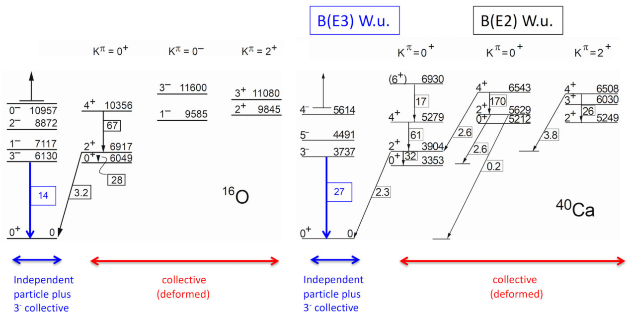
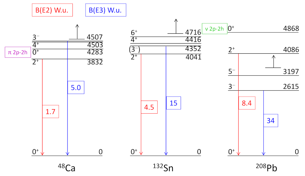
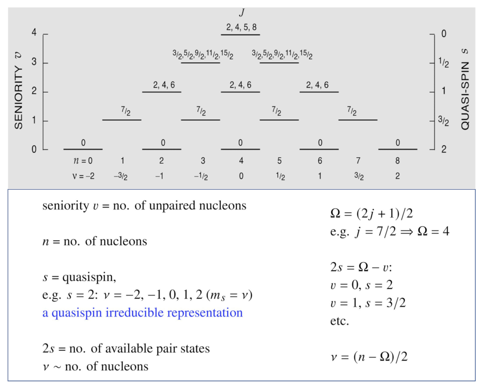
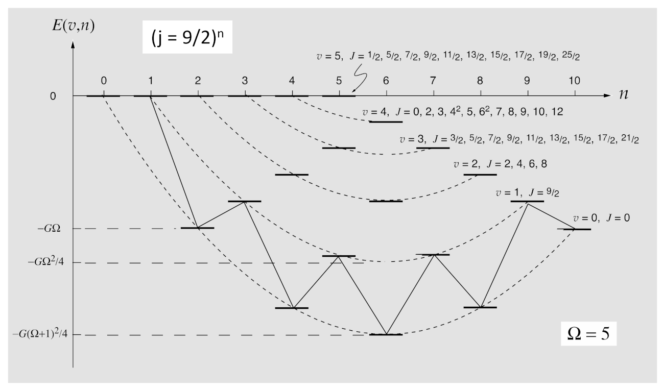
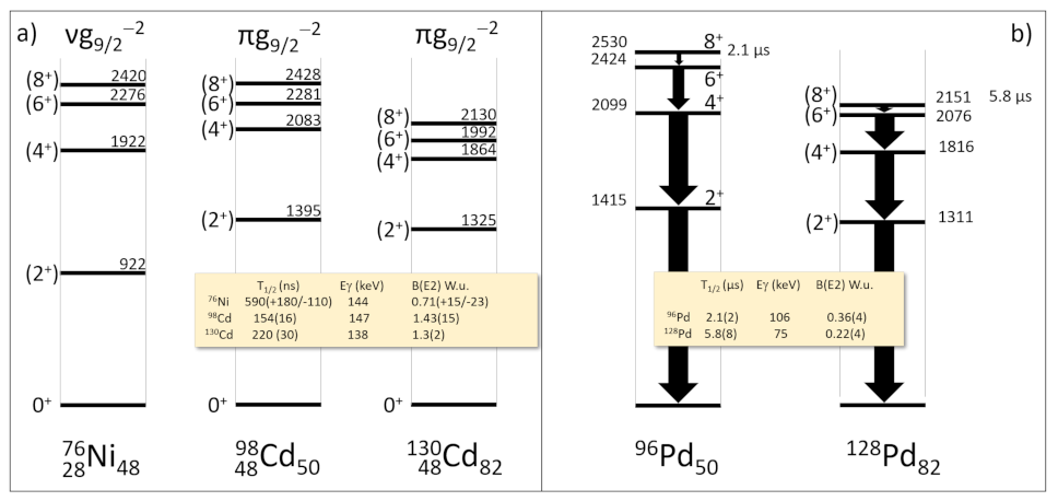
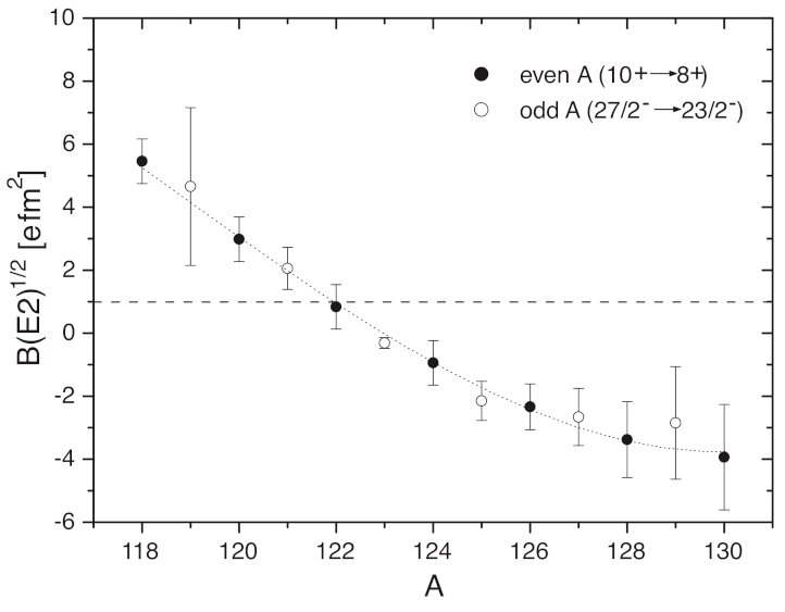
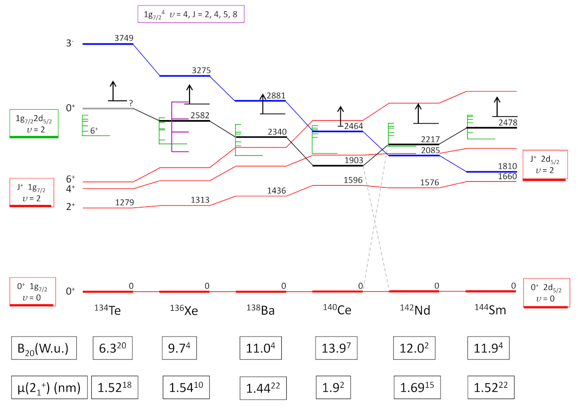
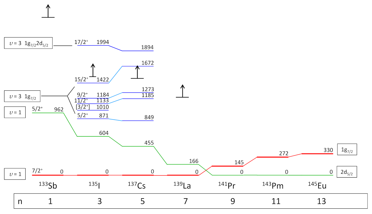
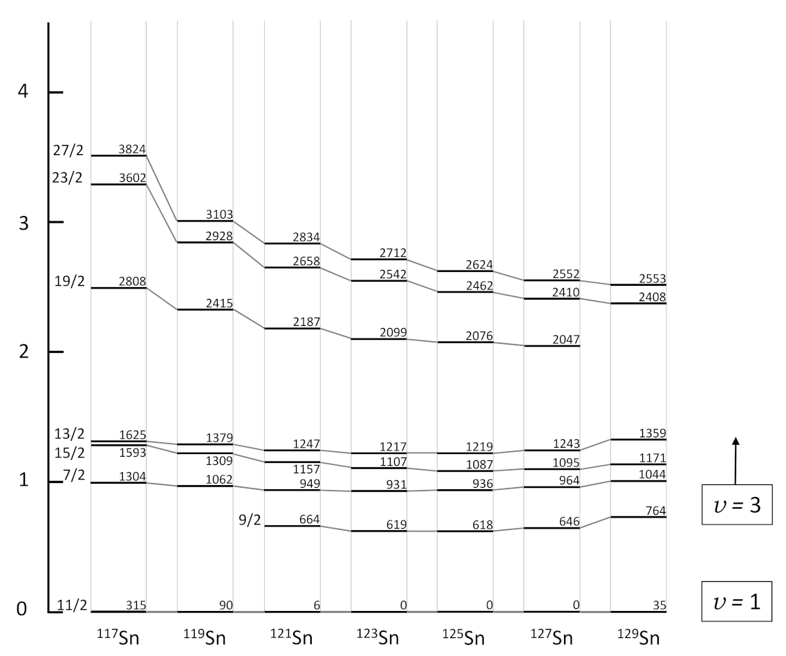
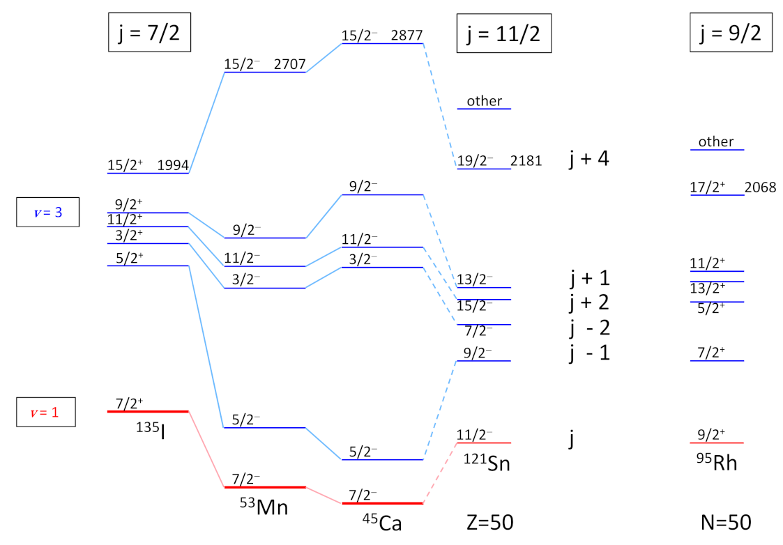
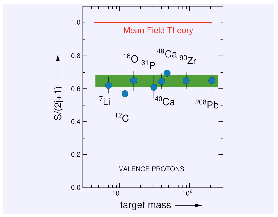
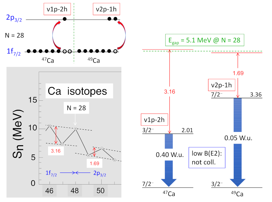
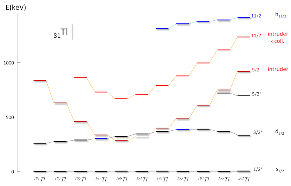
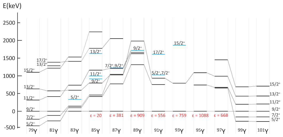
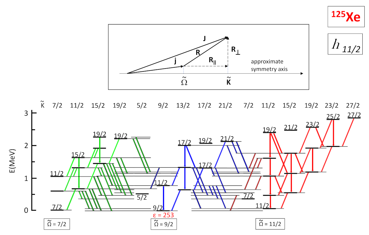
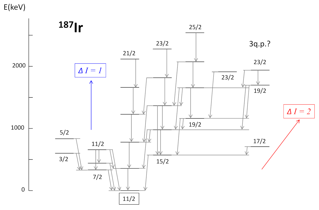
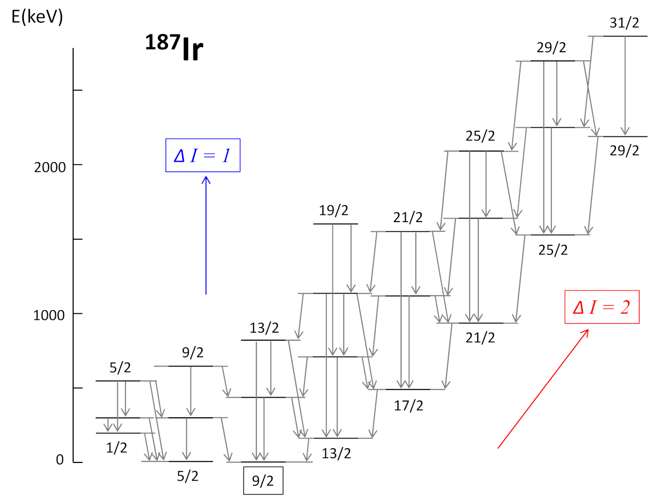
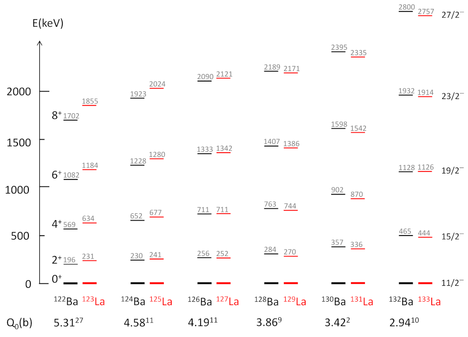
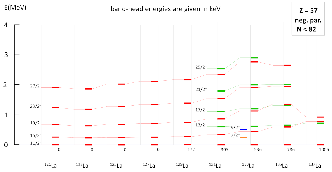
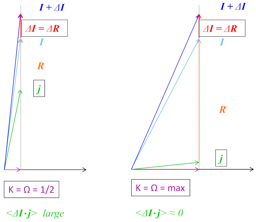
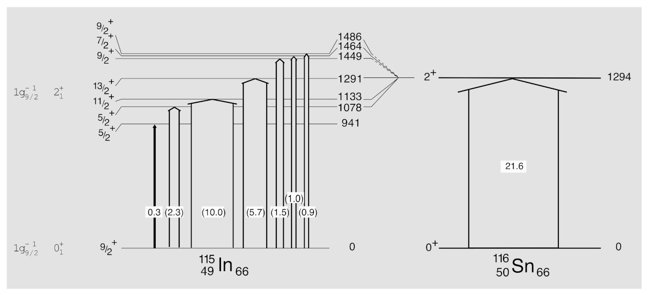
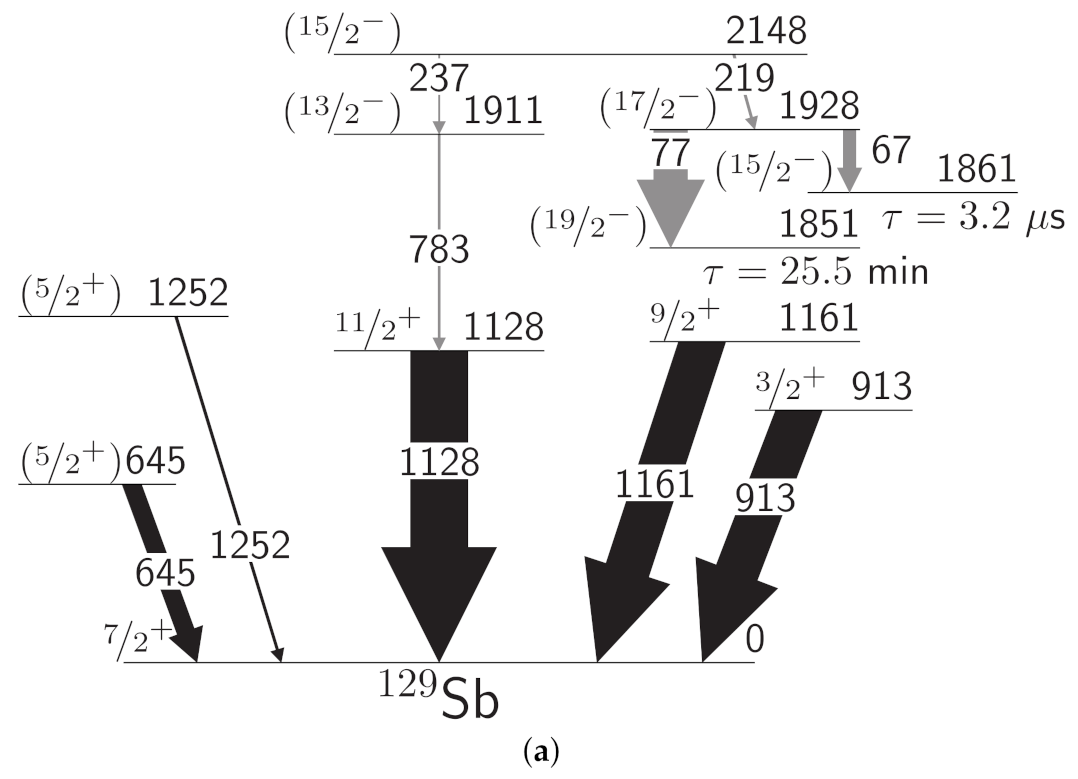
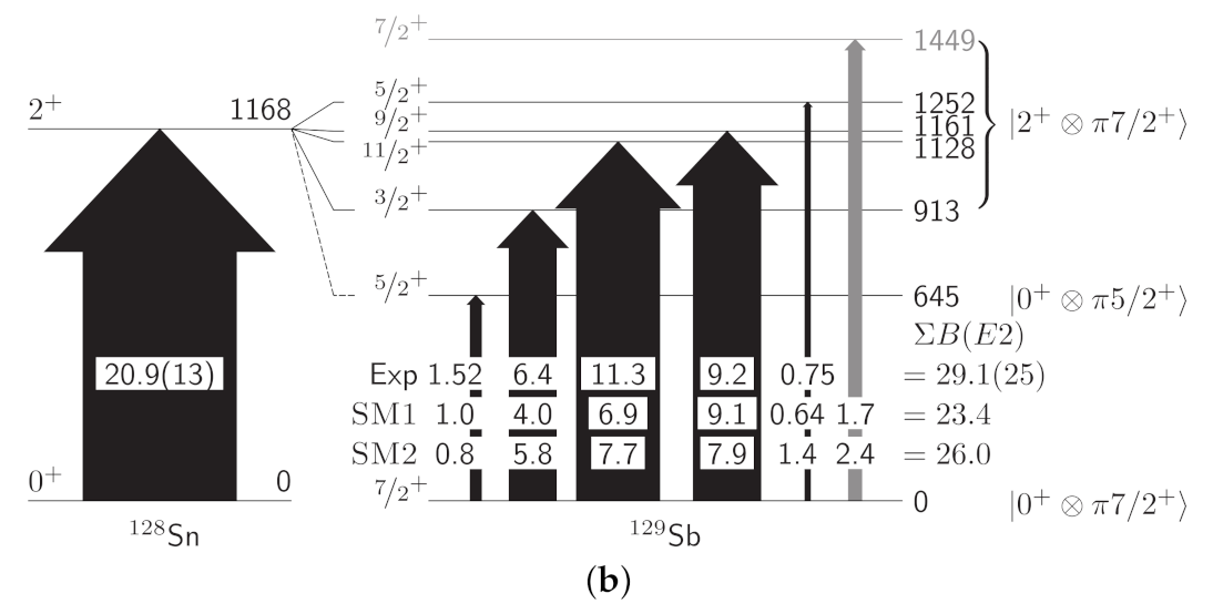
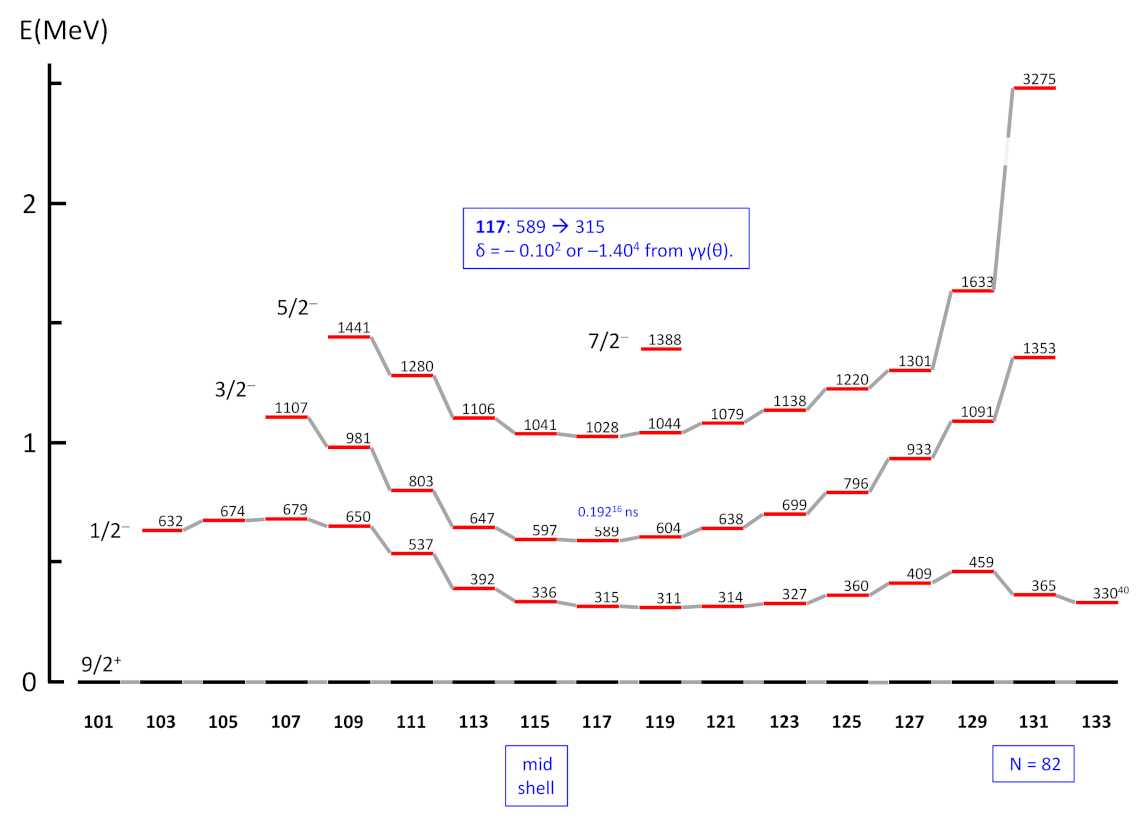
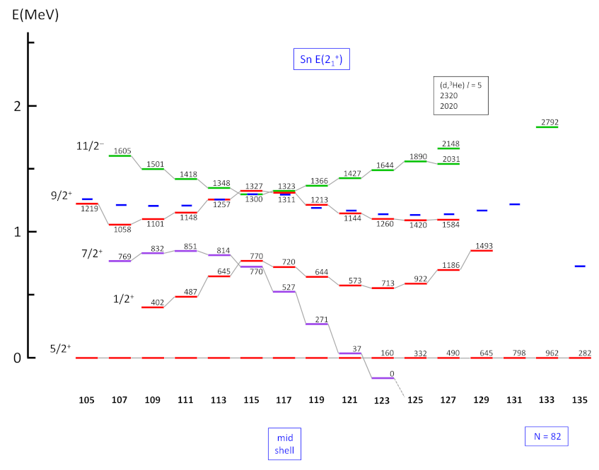
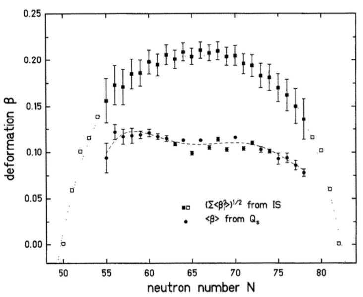
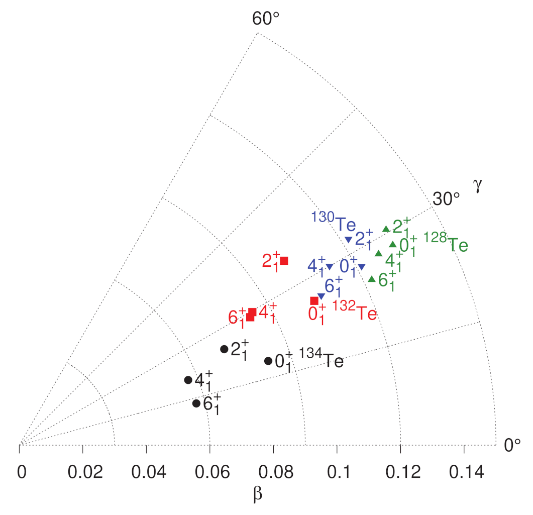
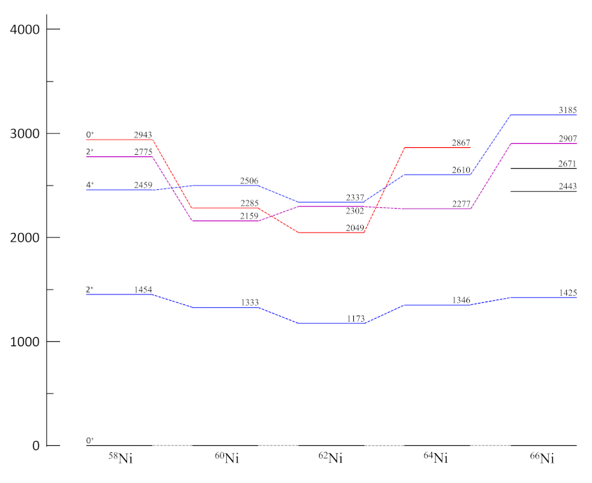
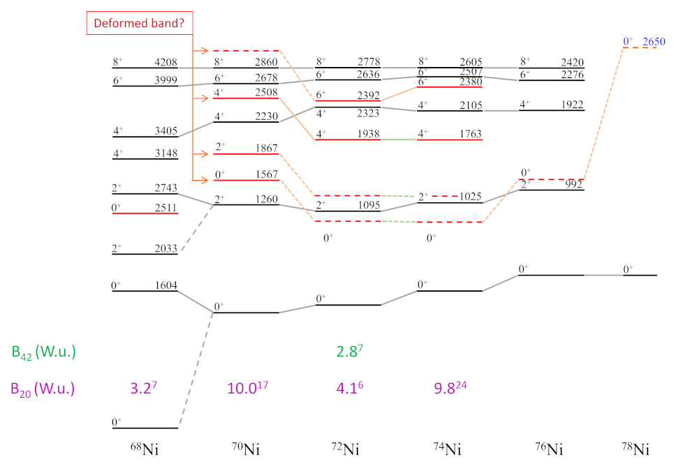
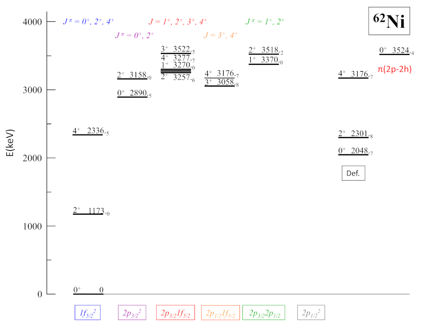
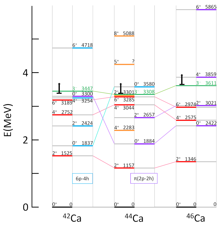
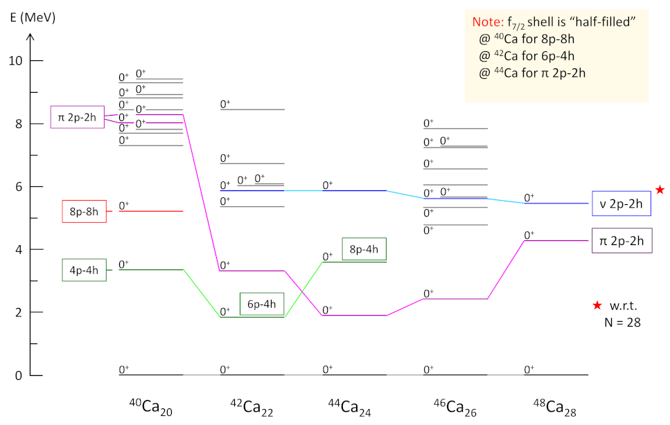
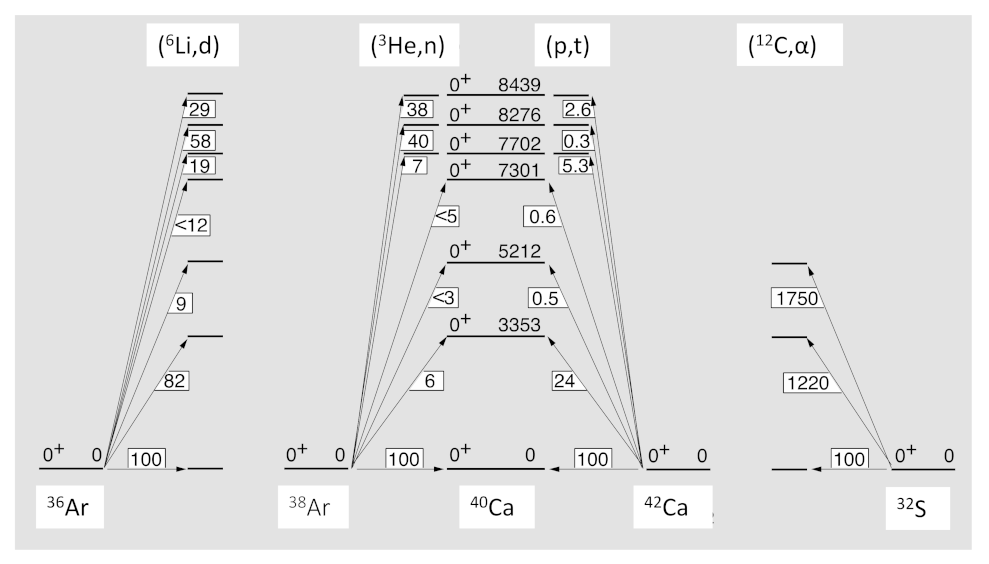
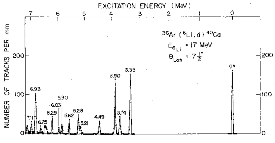
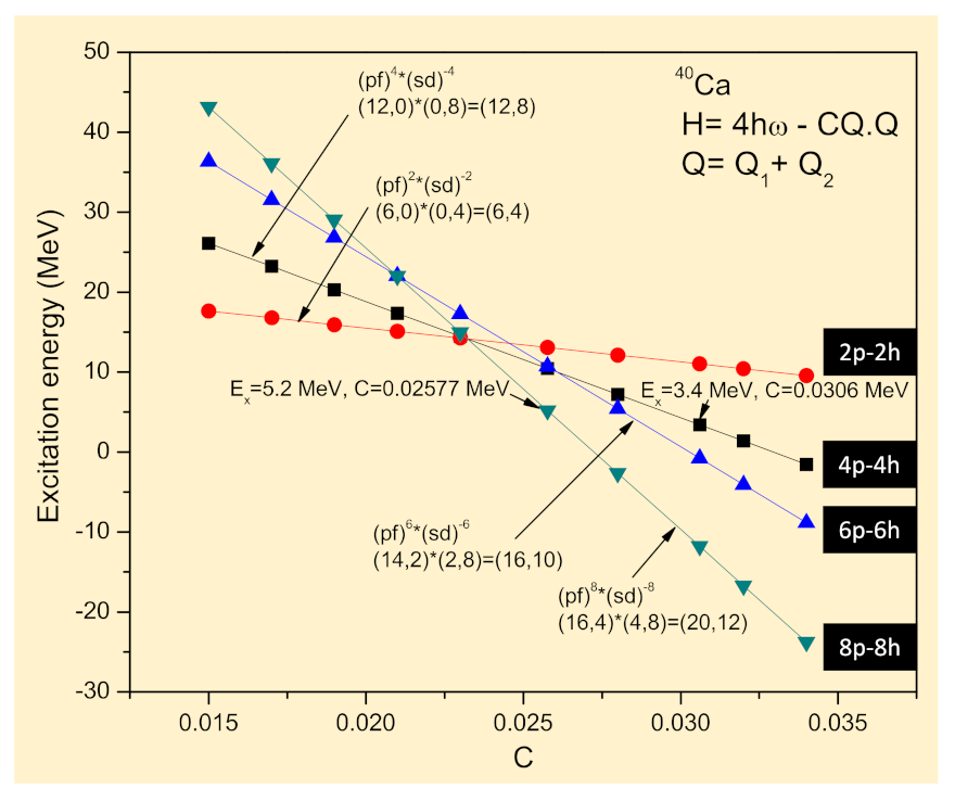
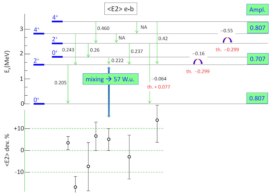
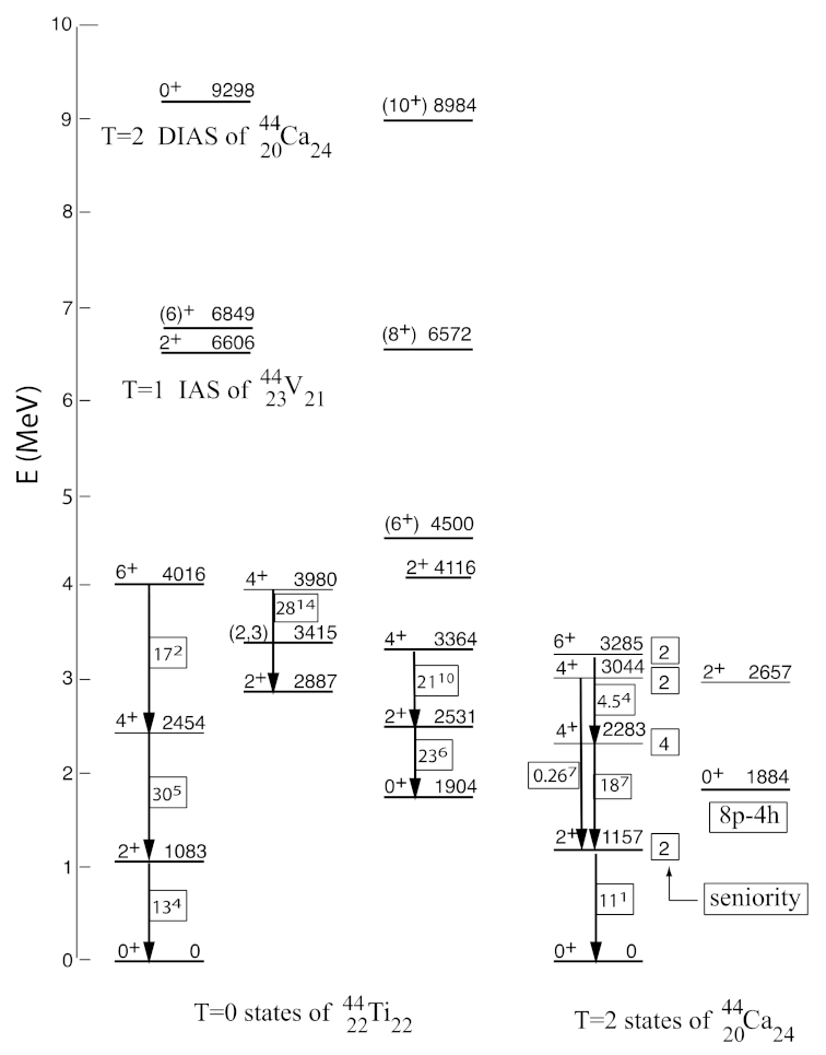
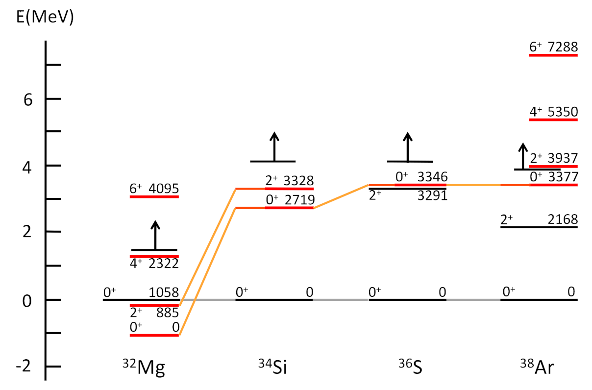
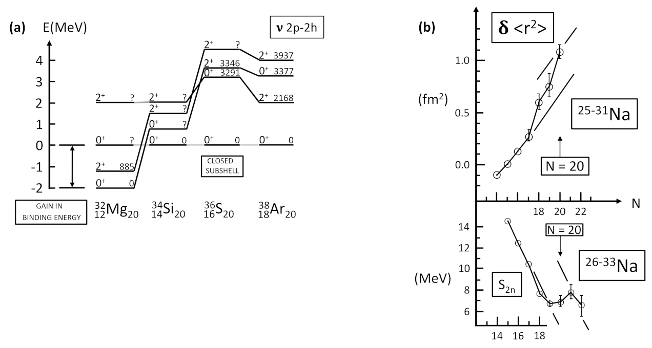
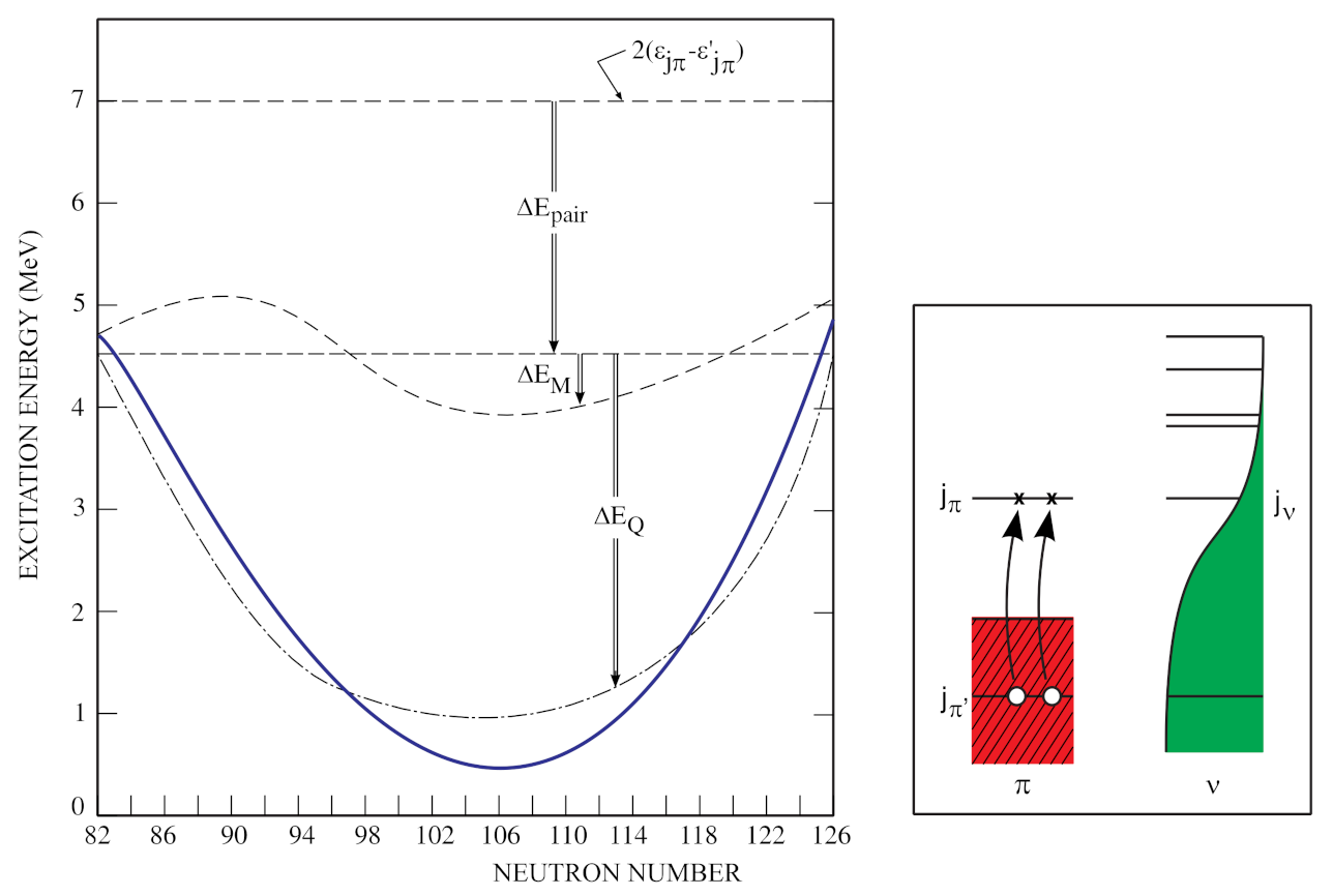
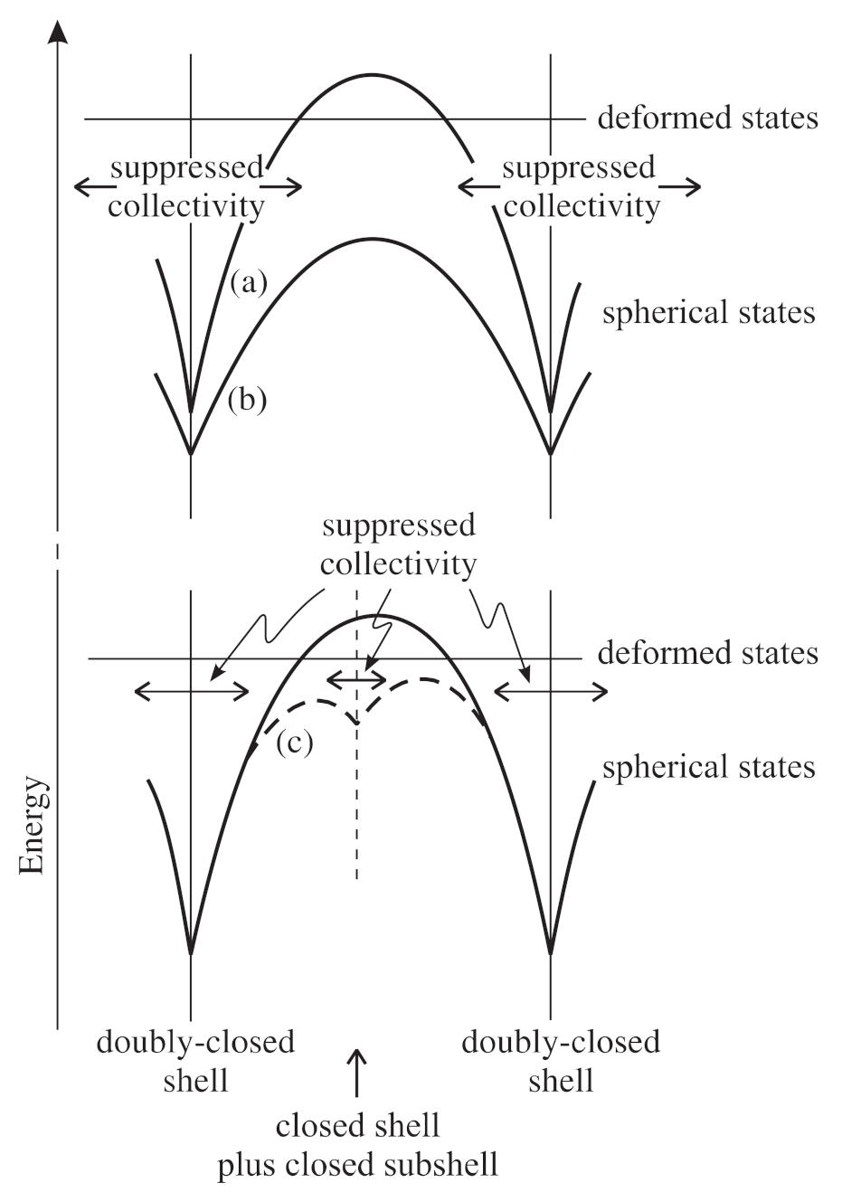
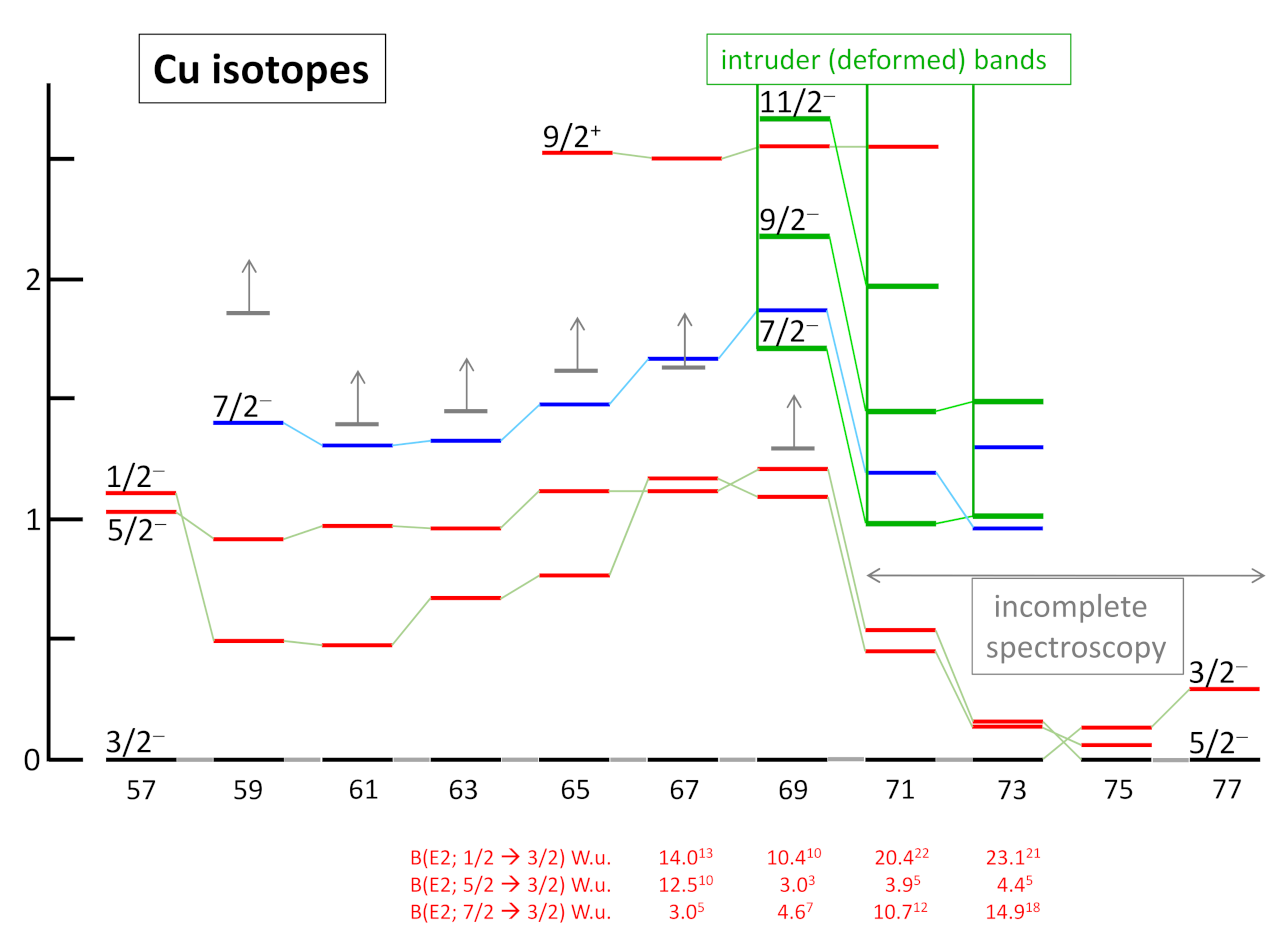
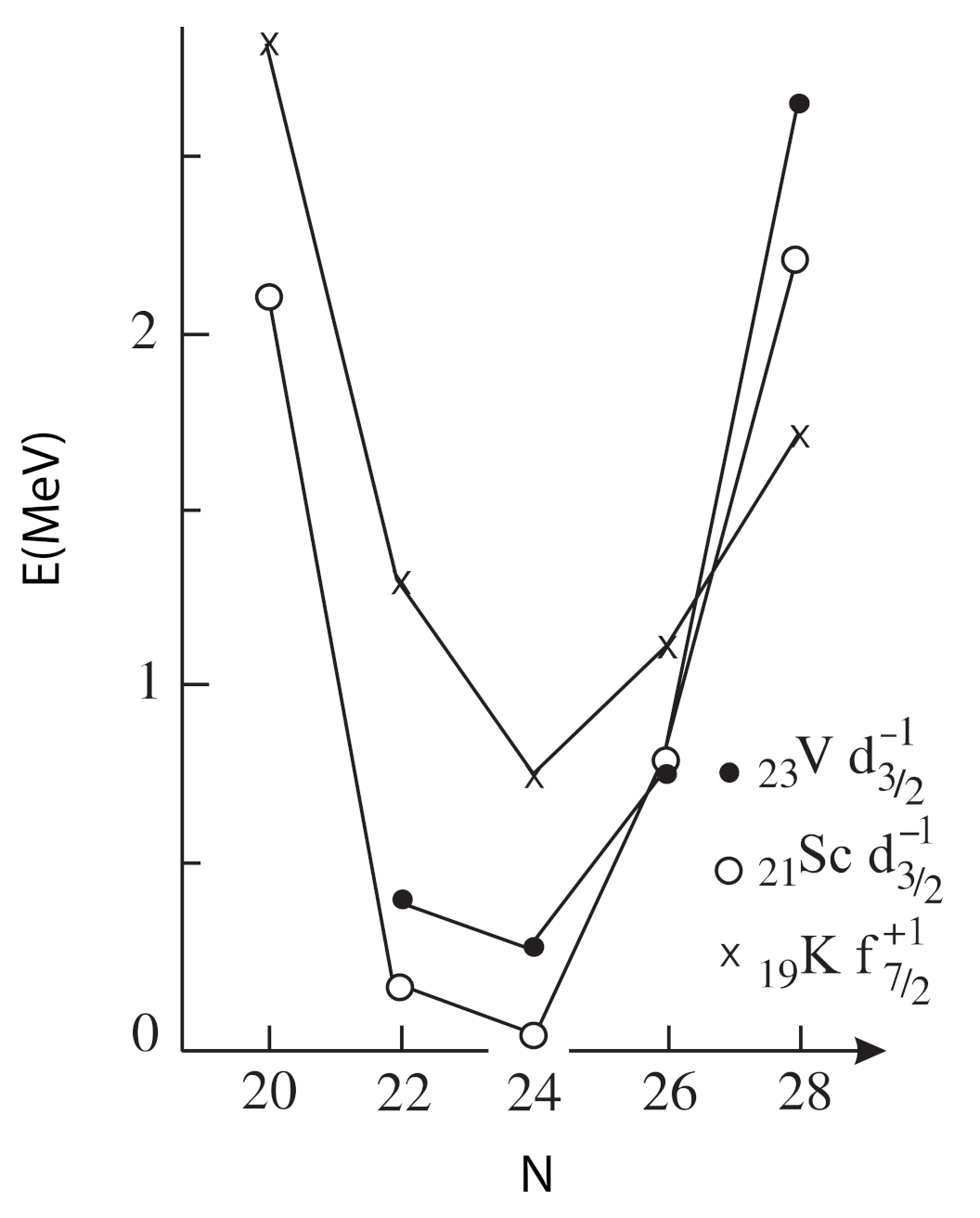
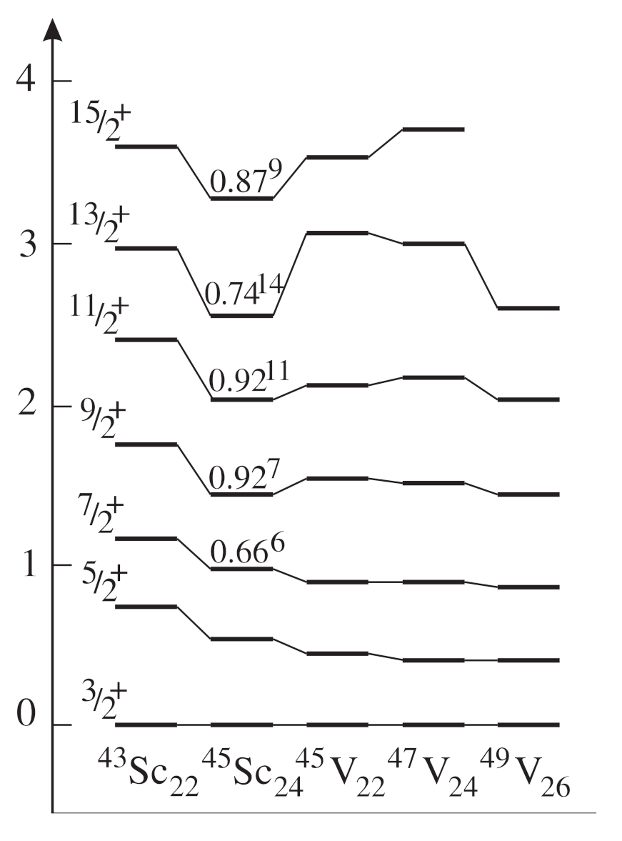
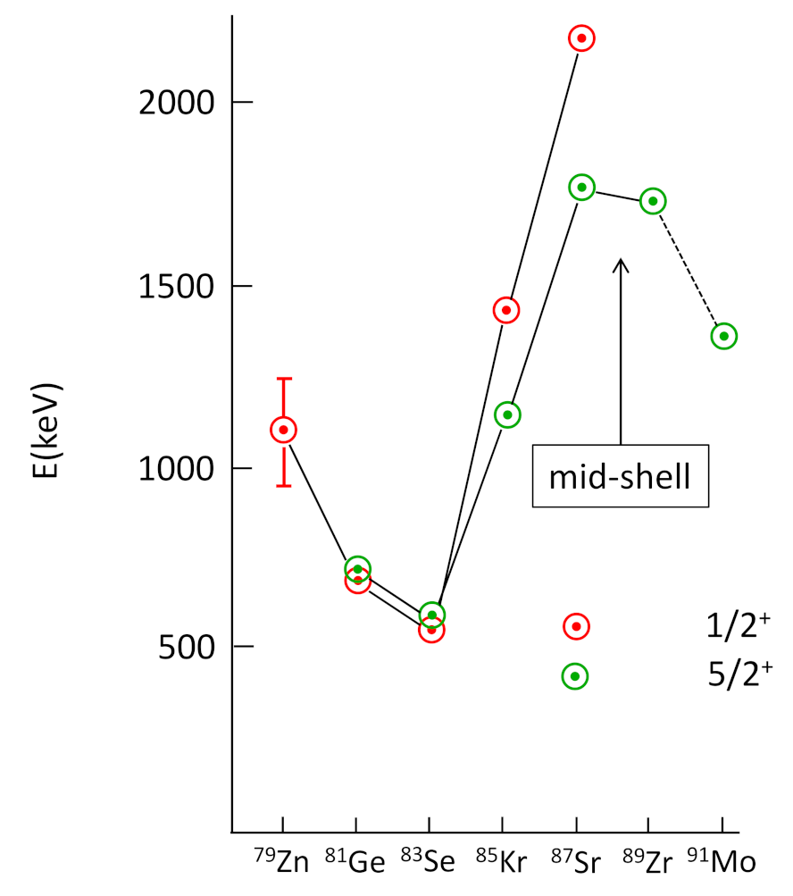
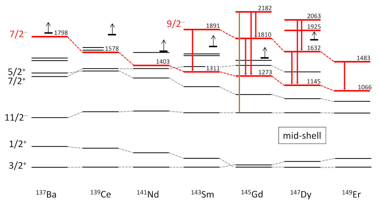
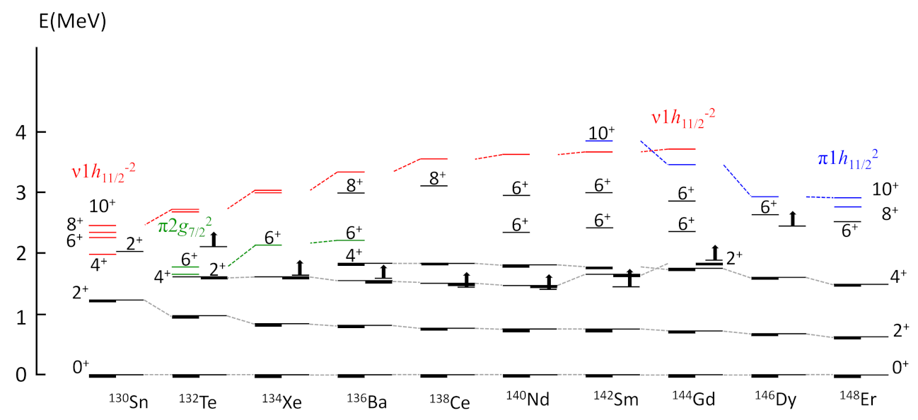
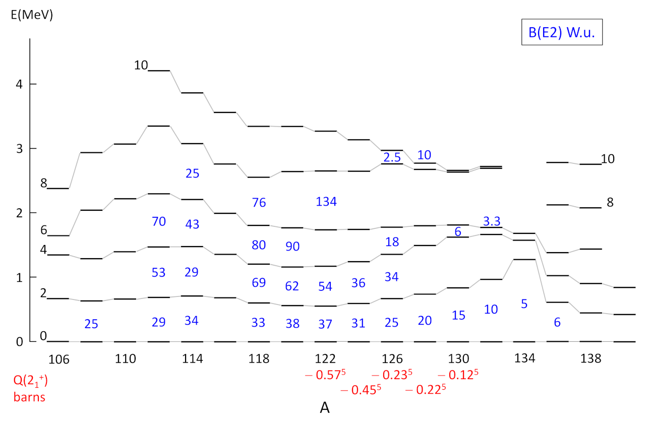
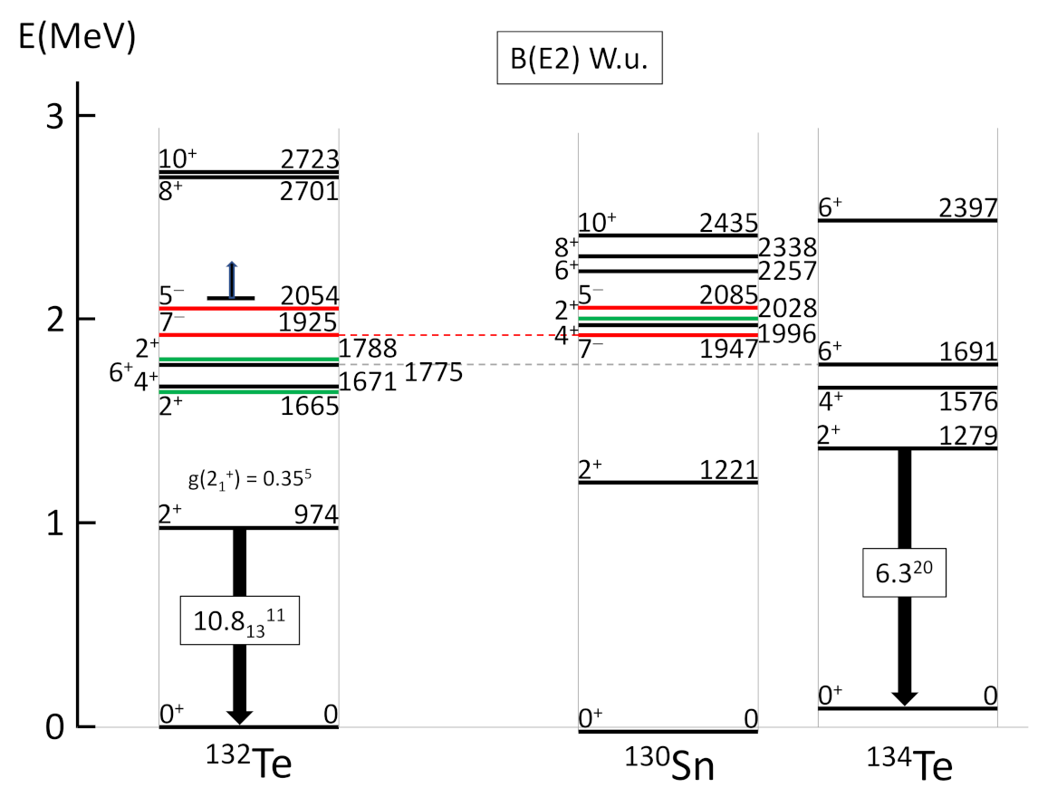
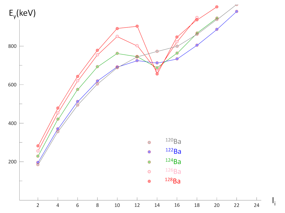
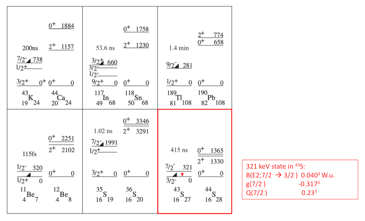
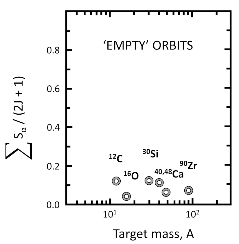