Emerging Concepts in Nuclear Structure Based on the Shell Model


1
RIKEN Nishina Center, 2-1 Hirosawa, Wako, Saitama 351-0198, Japan
2
Department of Physics, The University of Tokyo, 7-3-1 Hongo, Bunkyo, Tokyo 113-0033, Japan
3
Advanced Science Research Center, Japan Atomic Energy Agency, Tokai, Ibaraki 319-1195, Japan
Physics 2022, 4(1), 258-285; https://doi.org/10.3390/physics4010018
Submission received: 5 January 2022
/
Revised: 31 January 2022
/
Accepted: 8 February 2022
/
Published: 22 February 2022
(This article belongs to the Special Issue The Nuclear Shell Model 70 Years after Its Advent: Achievements and Prospects)
Abstract
:Some emerging concepts of nuclear structure are overviewed. (i) Background: the many-body quantum structure of atomic nucleus, a complex system comprising protons and neutrons (called nucleons collectively), has been studied largely based on the idea of the quantum liquid (à la Landau), where nucleons are quasiparticles moving in a (mean) potential well, with weak “residual” interactions between nucleons. The potential is rigid in general, although it can be anisotropic. While this view was a good starting point, it is time to look into kaleidoscopic aspects of the nuclear structure brought in by underlying dynamics and nuclear forces. (ii) Methods: exotic features as well as classical issues are investigated from fresh viewpoints based on the shell model and nucleon–nucleon interactions. The 70-year progress of the shell–model approach, including effective nucleon–nucleon interactions, enables us to do this. (iii) Results: we go beyond the picture of the solid potential well by activating the monopole interactions of the nuclear forces. This produces notable consequences in key features such as the shell/magic structure, the shape deformation, the dripline, etc. These consequences are understood with emerging concepts such as shell evolution (including type-II), T-plot, self-organization (for collective bands), triaxial-shape dominance, new dripline mechanism, etc. The resulting predictions and analyses agree with experiment. (iv) Conclusion: atomic nuclei are surprisingly richer objects than initially thought.
1. Introduction
The atomic nucleus is in a unique position in physics in that it is an isolated object but comprises many quantum ingredients. Some emerging concepts for the structure of atomic nuclei are overviewed in this paper, focusing on the works in which the author was involved. Obviously, those concepts have been found or clarified thanks to the great progress of nuclear-structure physics over 70 years, including the shell model.
In fact, the understanding of nuclear structure is based, to a great extent, on the shell model, which was introduced by Mayer [1] and Jensen [2] in 1949. Since then, the shell model has been developed significantly in many ways: an initial phase as many-body physics was presented, for instance, by Talmi in [3], in contrast to Mayer-Jensen’s independent-particle model. The subsequent developments are reviewed, for instance by Caurier et al. in [4] up to 2005, and in this volume up to date. I would like to sketch emerging concepts of nuclear structure based on recent shell–model studies involving the author, as many other studies are to be presented in other papers of the same volume.
The atomic nucleus comprises Z protons and N neutrons. Their sum is called the mass number . Among atomic nuclei, stable nuclei are characterized by their infinite or practically infinite life times and are characterized by rather balanced Z to N ratios, with ranging from about 1 up to about 1.5. There are about 300 nuclear species of this category. Other nuclei are called exotic (or unstable) nuclei. The total number of them is unknown but seems to be between 7000 and 10,000, providing a huge show window of various features as well as the paths of nucleosynthesis in the cosmos (see, for instance, [5,6,7]). The exotic nuclei decay, by (i.e., weak) processes, to other nuclei where Z and N are better balanced, as the decay alters a neutron to a proton or vice versa. This decay occurs successively, until the process terminates at a stable nucleus. Thus, only stable nuclei exist on earth, while exotic nuclei do not, being exotic literally.
Some of the emerging concepts were conceived in the study of exotic nuclei, particularly by looking at the shell structure and magic numbers of them. The obtained concepts were found later not to be limited to exotic nuclei. In this way, after the initial trigger by exotic nuclei, the overall picture of the nuclear shell structure has been renewed, and Section 2 of this paper is devoted to a sketch of it with two major keywords, the monopole interaction and the shell evolution.
We then focus on the deformation of the nuclear surface. The surface deformation from the sphere has been a very important subject since the 1950s, as initiated by Rainwater [8] and by Bohr and Mottelson in [9,10,11,12,13]. In particular, the shape coexistence phenomenon is discussed as the crossroad between the shell evolution and the deformation, leading to the concept of type-II shell evolution. Although I do not discuss extensively the methodology of the shell model calculation in this paper because of the length limitation, the T-plot of the Monte Carlo Shell Model (MCSM) is mentioned as an essential theoretical tool for many physics cases of this paper. These are the main subjects of Section 3.
The in-depth clarification of the collective band is connected to the fundamental question on the relation between the single-particle degrees of freedom and the collective motion of nucleons. These two must be connected through nuclear forces. This question has not been clarified enough as also addressed by G. E. Brown [14]. I shall focus, in Section 4, on how this question may be understood more deeply, by introducing the self-organization aspect of the collective bands and by raising the importance of the triaxiality of nuclear shapes including the ground states.
The interplay between the monopole interaction and the quadrupole deformation is shown to be a major mechanism of the determination of the neutron driplines. This approach explains neutron driplines observed recently. We are led to two dripline mechanisms: the traditional one with the single-particle origin and the present one. The monopole–quadrupole interplay responsible for this new dripline mechanism is explained in detail in Section 5. As an alternative case, spherical isotopes, such as Ca, Ni, Sn, and Pb, are predicted to exhibit a different pattern.
The intention of this paper is to show the major flow of basic ideas and related results without going into details. I hope that the reader can grasp this flow and could become interested in watching further developments. The past 70 years are really great for the shell model, but the coming years look equally or even more brilliant. I apologize for not covering many of the major developments in the last 70 years, as such coverage is not possible within this paper, but the other contributions of this volume are expected to help.
2. Shell Evolution Due to Monopole Interaction
2.1. Mayer–Jensen’s Shell Model and Observed Magic Numbers
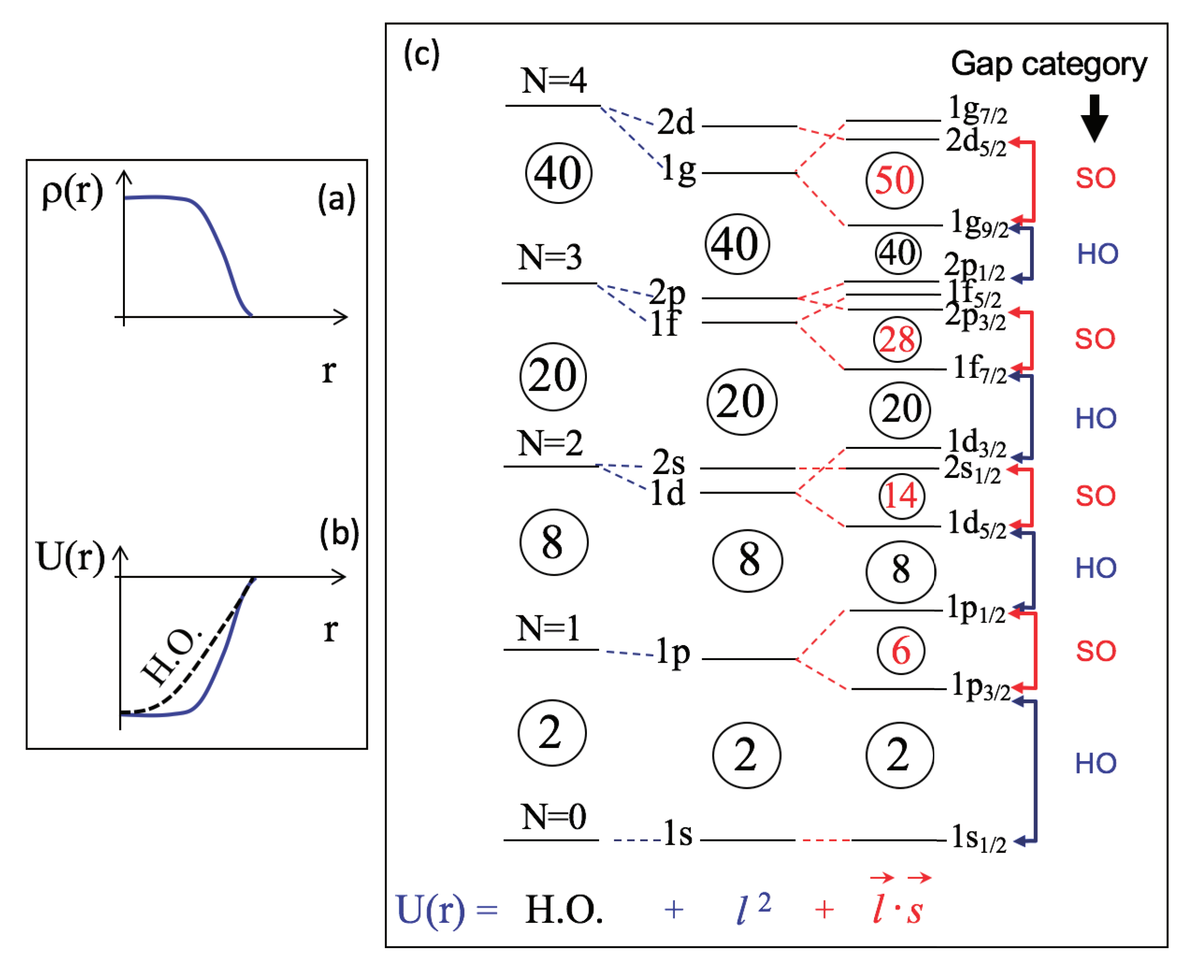
Mayer [1] and Jensen [2] proposed, in 1949, the model of the shell structure and magic numbers of atomic nuclei. This model provided major guides for a deeper and wider understanding of the structure of atomic nuclei. While this is a similar situation to electrons in atoms, there are some differences. Figure 1 depicts the basic idea and consequences of the Mayer–Jensen’s scheme. We start with the nuclear matter composed of protons and neutrons. This matter shows an almost constant density of nucleons (collective name of protons and neutrons) inside the surface, which is a sphere as a natural assumption (see Figure 1a). Because of the short-range character of nuclear forces, this constant density results in a mean potential with a constant depth inside the surface, as shown in Figure 1b. Let us assume that the density distribution is isotropic, producing an isotropic mean potential. Figure 1b also suggests that the Harmonic Oscillator (HO) potential is a good approximation to this mean potential as long as the mean potential shows negative values as a function of r, the radius from the center of the nucleus. We then switch from the mean potential to the HO potential, which is analytically more tractable. Thus, the HO potential can be introduced from the constant density (sometimes referred to as “density saturation”) and the short-range attraction due to nuclear forces.
The eigenstates of the HO potential are single-particle states shown in the far-left column of Figure 1c with associated magic numbers and HO quanta, N. These HO magic numbers do not change by adding the minor correction of the term, the scalar product of the orbital angular momentum (see the second column from left in Figure 1c; for details see [12]).
The crucial factor introduced by Mayer and Jensen was the spin-orbit (SO) term, , the effect of which is shown in the third column from the left in Figure 1c. The two orbits with the same orbital angular momentum, ℓ, and the same HO quanta are denoted as,
where is due to the spin, s = 1/2. The notation of and is used frequently in this paper. The spin-orbit term,
is added to the HO + potential, where f is the strength parameter. With as is the case for nuclear forces, the state is lowered in energy, whereas the state is raised. The value of f is known empirically to be about −20 MeV (see Equation (2-132) of [12]).
The final pattern of the single-particle energies (SPE) is shown schematically in Figure 1c. The single-particle states are labeled in the standard way up to their j values, and both HO and spin-orbit magic gaps are indicated in black and red, respectively. The magic numbers have been considered to be = 2, 8, 20, 28, 50, 82, and 126, because the effect of the spin-orbit term becomes stronger as j becomes larger. In fact, the magic numbers 28, 50, 82, and 126 are all due to this effect. Instead, the HO magic numbers beyond 20 were considered to be absent or show only minor effects. We shall look back on them, from modern views of the nuclear structure covering stable and exotic nuclei.
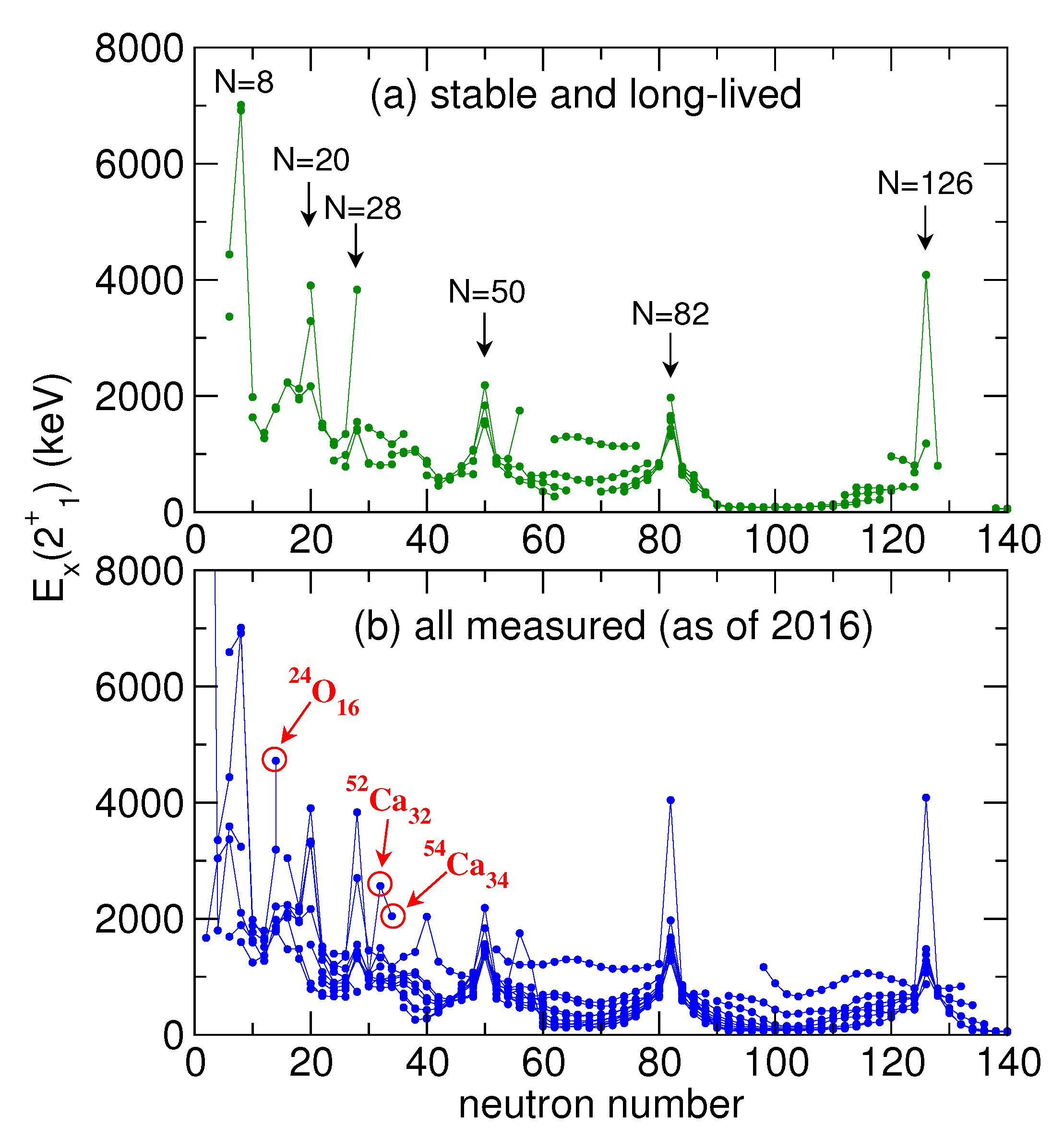
We now investigate to what extent magic gaps in Figure 1c have been observed. Figure 2 displays the observed excitation energies of the first 2+ states of even-even nuclei as a function of N, where even-even stands for even-Z-even-N. These excitation energies tend to be high at the magic numbers, because excitations across the relevant magic gap are needed. The conventional magic numbers of Mayer and Jensen, N = 2, 8, 20, 28, …126 are expected to arise, and we indeed see sharp spikes at these magic numbers in Figure 2a where the excitation energies are shown for stable and long-lived (i.e., meta stable) nuclei. Figure 2b includes all measured first 2+ excitation energies as of 2016. In addition to the spikes in Figure 2a, one sees some new ones. One of them is at N = 40, which corresponds to 68Ni40, representing a HO magic gap at N = 40. There are three others corresponding to the nuclei, 24O16, 52Ca32, and 54Ca34, as marked in red. The 2+ excitation energies of these nuclei are about a factor of two higher than the overall trend, suggesting that N = 16, 32 and 34 can be magic numbers, although none of them is present in Figure 1c.
These new possible magic numbers are consequences of what are missing in the argument for deriving magic gaps in Figure 1c. We now turn to follow some passages along which this subject has been studied.
2.2. Monopole Interaction
The change from the Mayer–Jensen scheme is discussed from the viewpoint of the nucleon-nucleon () interaction. The Hamiltonian is written as,
where denotes the one-body term given by
and stands for the interaction. Here, means the proton- or neutron-number operator for the orbit j, and implies proton or neutron SPE of the orbit j. This SPE is composed of the kinetic energy of the orbit j and the binding energy on the orbit j generated by all nucleons in the inert core. We note that the interaction in Equation (3) can be any interaction between two nucleons in the following discussions but actually refers to effective interactions between valence (i.e., active) nucleons.
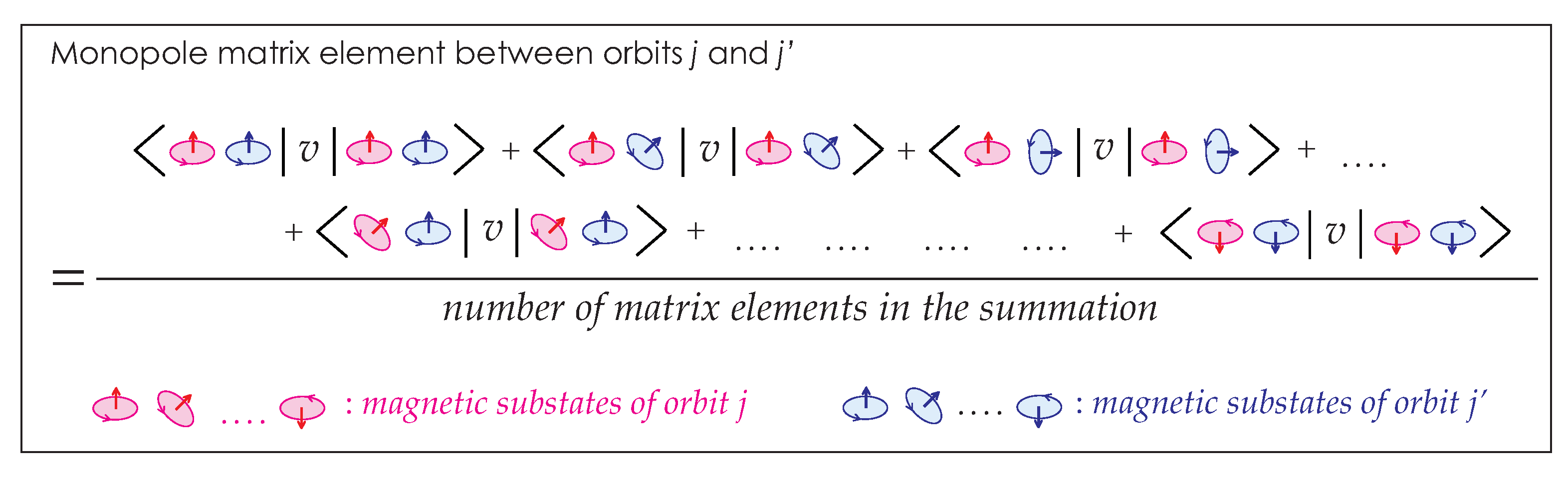
The interaction can be decomposed, in general, into the two components: monopole and multipole interactions [17], irrespectively of its origin, derivation, or parameters. The monopole interaction, denoted as , is expressed in terms of the monopole matrix element, which is defined for single-particle orbits j and as,
where m and are magnetic substates of j and , respectively, and the summation over is taken for all ordered pairs allowed by the Pauli principle. The monopole matrix element represents, as displayed schematically in Figure 3, an orientation average for two nucleons in the orbits j and . See [15] for more detailed descriptions.
The monopole interaction between two neutrons is then given as
The monopole interaction between two protons is given similarly. The monopole interaction between a proton and a neutron can be given as
where stands for the monopole matrix element for the isospin T = 0 or 1 channel, respectively, defined by Equation (5) including isospin-symmetry effects (see Sec. III A of Ref. [15] for details). Note that implies . The second term on the right-hand-side (r.h.s.) of Equation (7) is slightly different from the first term on the r.h.s. of Equation (7) due to the special isospin property for the cases of j = . Obviously, can be rewritten as
with defined so as to reproduce Equation (7).
The functional forms in Equations (6) and (8) appear to be in accordance with the intuition from the averaging over all orientations: no dependencies on angular properties (e.g., coupled J values) between the two interacting nucleons and the sole dependence on the number of particles in those orbits.
The (total) monopole interaction is written as
and the monopole Hamiltonian is defined as,
The multipole interaction is introduced as
and the (total) Hamiltonian is written as . The multipole interaction becomes crucial in many aspects of nuclear structure, for instance, the shape deformation, as touched upon in later sections of this article. The monopole interaction has been studied over decades with many works, for example, [17,18,19,20] (see [15] for more details).
We define the effective SPE (ESPE) of the proton (neutron) orbit j, denoted by (), as the change of the monopole Hamiltonian, in Equation (10), due to the addition of one proton (neutron) into the orbit j. This change is nothing but the difference, when is replaced by +1. For instance, the first term on the r.h.s. of Equation (10) contributes to by a constant, . As another example, the r.h.s. of Equation (8) contributes by . Combining all terms, the ESPE of the proton orbit j is given as,
The second and third terms on the r.h.s. are obviously contributions from valence protons and neutrons, respectively. The neutron ESPE is expressed similarly as
In many practical cases, an appropriate expectation value of the ESPE operator is also called the ESPE with an implicit reference to some state characterizing the structure, e.g., the ground state.
The ESPE as an expectation value is often discussed in terms of the difference between two states, e.g., and . The states and may belong to the same nucleus or to two different nuclei. We here show the formulas for this difference. First we introduce the symbol for an operator implying the difference, . Such differences of the ESPE values are expressed as,
and
If is a doubly closed shell and is an eigenstate with some valence protons and neutrons on top of this closed shell, these quantities stand for the evolution of ESPEs as functions of Z and N. One can thus see various physics cases represented by and . Such ESPEs can provide picturesque prospects and great help in intuitive understanding without resorting to complicated numerical calculations. The notion of the ESPE has been well utilized, for instance, in empirical studies in [6,21], in certain ways related to the present article.
The interaction can be decomposed into several parts according to some classifications. The discussions in this subsection can then be applied to each part separately: the monopole interaction of a particular part of can be extracted, and its resulting ESPEs can be evaluated. Examples are presented in the subsequent subsections.
We note that the definition of the ESPE can have certain variants with similar consequences, for instance, the combination of and instead of and . Appendix A shows a note on the relation to Baranger’s ESPE.
2.3. Central, Two-Body Spin-Orbit and Tensor Parts of the NN Interaction
With these formulations, we can discuss a variety of subjects ranging from the shell structure, to the collective bands, and to the driplines. Let us start with the shell structure. While the discussions in Section 2.1 are based on basic nuclear properties, some aspects are missing. One of them is the orbital dependencies of the monopole matrix element. This dependence generally appears but shows up more crucially in certain cases.
As we shall see, some parts of the interaction, , show characteristic and substantial orbital dependencies. Such parts can be specified in terms of their spin properties, as the interaction involves a spin operator, an axial vector of nucleon. We first take the part where no spin operator is included or spin operators are coupled to scalar terms, like with denoting the spin operator of the nucleon 1 or 2, and being a scalar product. This part is called the central force, and its effects are discussed in Section 2.4. In the second part, spin operators are coupled to axial vectors. Such axial vectors must be coupled with other axial vectors such as the orbital angular momentum. The two-body spin-orbit force belongs to this case, and its effects are discussed in Section 2.8, while the effects remain quite modest except for special orbital combinations. As presented in Section 2.5, significant contributions arise from the tensor force, where spin operators are coupled to a (rank-2) tensor, , where the last superscript means rank 2. This is a very complicated coupling, and this term must be coupled, in the interaction, with another (rank-2) tensor of the coordinates, in order to form a scalar. Similar terms appear in the electromagnetic interaction, but their effects are minor. The tensor force is, however, crucial in the nuclear case, because the pion exchange process produces it as its primary source. Section 2.5 presents monopole properties of the lowest-order contribution of the tensor force, while higher-order contributions are largely included in the central force of the effective interaction mentioned above.
2.4. Monopole Interaction of the Central Force
We now discuss the monopole interaction of the central-force component of interactions. Because the interaction is characterized by intermediate-range (∼1 fm) attraction after modifications or renormalizations, the monopole matrix elements gain large magnitudes with a negative sign (i.e., attractive), if radial wave functions of the single-particle orbits, j and in Equation (5), are similar to each other. This similarity is visible, if these orbits are spin-orbit partners ( and ) with the identical radial wave functions (see Equation (1)), for instance and . Another example is the coupling between unique-parity orbits, such as and , for which the radial wave functions are similar because of no radial node. These types of strong correlations were pointed out by Federman and Pittel in [22], where the total effect of the 3S1 channel of the interaction was discussed without the reference to the monopole interaction.
2.5. Monopole Interaction of the Tensor Force
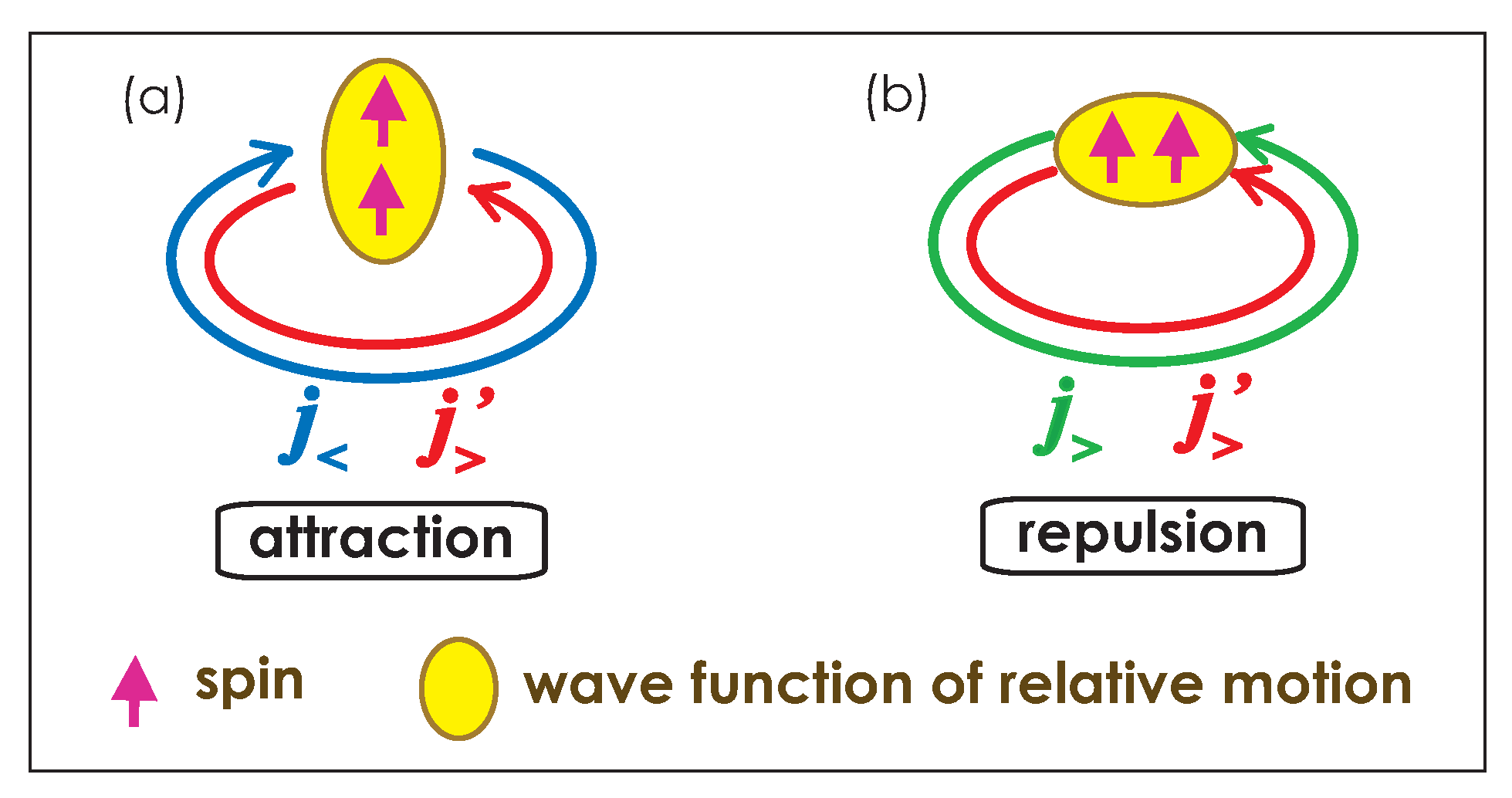
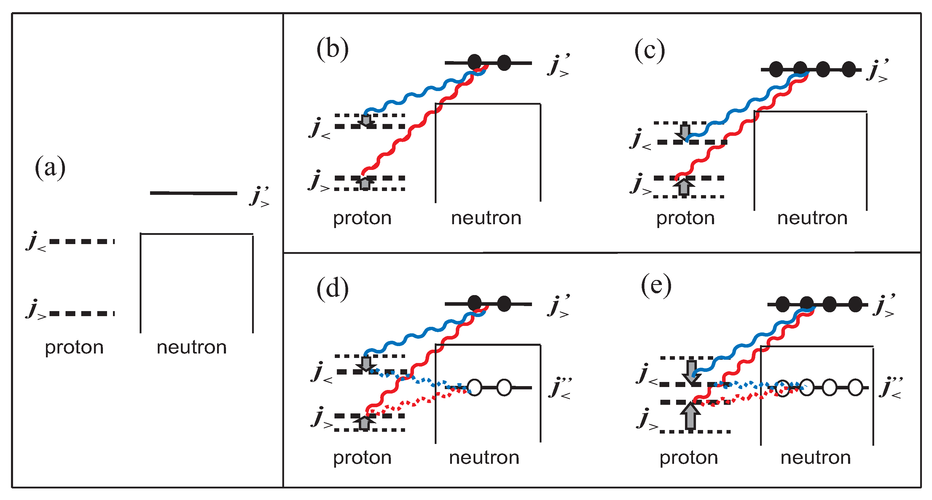
Another important source of the monopole interaction with strong orbital dependences is the tensor force. The tensor force produces very unique effects on the ESPE. This is shown in Figure 4: the intuitive argument in [15,23] proves that the monopole interaction of the tensor force is attractive between a nucleon in an orbit and another nucleon in an orbit , whereas it becomes repulsive for combinations, (, ) or (, ). The magnitude of such monopole interaction varies also. For example, it is strong in magnitude between spin-orbit partners or between unique-parity orbits, etc. [15].
The ESPE is shifted in very specific ways as exemplified in Figure 5b: if neutrons occupy a orbit, the ESPE of the proton orbit is raised, whereas that of the proton orbit is lowered. This is nothing but a reduction in a proton spin-orbit splitting due to a specific neutron configuration. The amount of the shift is proportional to the number of neutrons in this configuration, as shown in Equation (14) and in Figure 5c. Other cases follow the same rule shown in Figure 4. These general features have been pointed out in [23] with an analytic formula and an intuitive description of its origin.
2.6. Monopole-Interaction Effects from the Central and Tensor Forces Combined
The combined effects of the central and tensor forces were discussed in [25] in terms of realistic shell–model interactions, USD [26], and GXPF1A [27]. These interactions were obtained in two steps: the starting point was given by microscopic G-matrix interactions proposed initially by Kuo and Brown [28,29], and as the second step, certain phenomenological improvements were made by the fit to large numbers of experimental energy levels. It is mentioned that some main features, for instance, the tensor-force component, remain unchanged by this fit [25]. Many other valuable shell–model interactions, for instance, KB3 [17], Kuo-Herling [30], sn100pn [31], and LNPS [32] interactions, have been constructed from the G-matrix interactions sometimes with refinements like monopole adjustments. It should be noticed that these shell–model interactions are derived microscopically to a large extent and that they should be distinguished from purely phenomenological interactions in earlier times, e.g., [33]. The M3Y interaction [34] is related to the G-matrix, too. We appreciate the original contribution of the G-matrix approach to the effective interaction [28,29].
The interaction was then introduced as a general and simple shell–model interaction. Its central part consists of Gaussian interactions with spin/isospin dependencies, and their strength parameters are determined so as to simulate the overall features of the monopole matrix elements of the central part of USD [26] and GXPF1A [27] interactions. Its tensor part is taken from the standard - and -meson exchange potentials [23,35,36]. Thus, the interaction is defined as a function of the relative distance of two nucleons with spin/isospin dependences, which enables us to use it in a variety of regions of the nuclear chart, as we shall see. A wide model space, typically a HO shell or more, is required in order to obtain reasonable results, though.
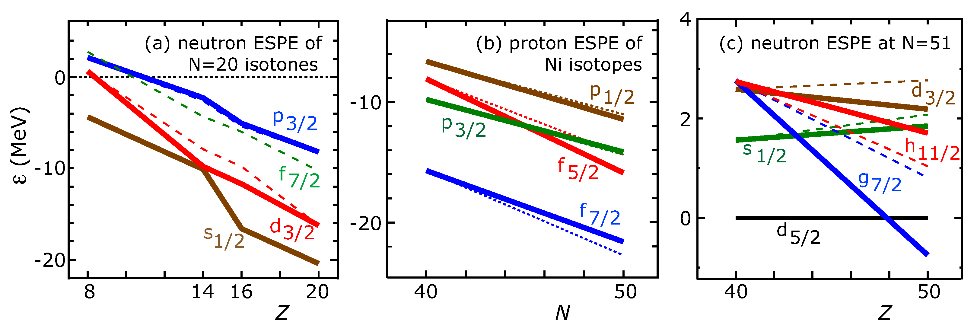
Figure 6 depicts some examples: Figure 6a displays the transition from a standard (à la Mayer–Jensen) N = 20 magic gap to an exotic N = 16 magic gap by plotting within the filling scheme (see Equation (13)), as Z decreases from 20 to 8. The tensor monopole interaction between the proton and the neutron orbits plays an important role. The small N = 20 magic gap for Z = 8–12 is consistent with the island of inversion picture (see reviews, e.g., [4,15]). Figure 6b depicts the inversion between the proton and orbits as N increases in Ni isotopes, by showing (see Equation (12)). The figure exhibits exotically ordered single-particle orbits for . The tensor monopole interactions between the proton and the neutron orbits produce crucial effects. Figure 6c shows significant changes in the neutron single-particle levels from 90Zr to 100Sn, in terms of . Without the tensor force, the approximate degeneracy of and orbits in 100Sn does not show up.
These changes in the shell structure as a function of Z and/or N were collectively called shell evolution in [23]. The splitting between proton and in Sb isotopes shows a substantial widening as N increases from 64 to 82 as pointed out by Schiffer et al. [37], which was one of the first experimental supports to the shell evolution partly because this was not explained otherwise. Note that while the origin of the shell evolution can be any part of the interaction, its appearance is exemplified graphically in Figure 5a–c for the tensor force. The shell-evolution trend depicted in Figure 6 appears to be consistent with experiment [15,25,38,39,40,41,42]. The monopole properties discussed in this subsection are consistent with the results shown by Smirnova et al. [43] obtained through the spin-tensor decomposition (see e.g., [15] for some account) for the “well-fitted realistic interaction for the sdpf shell–model space” [43].
2.7. N = 34 New Magic Number as a Consequence of the Shell Evolution
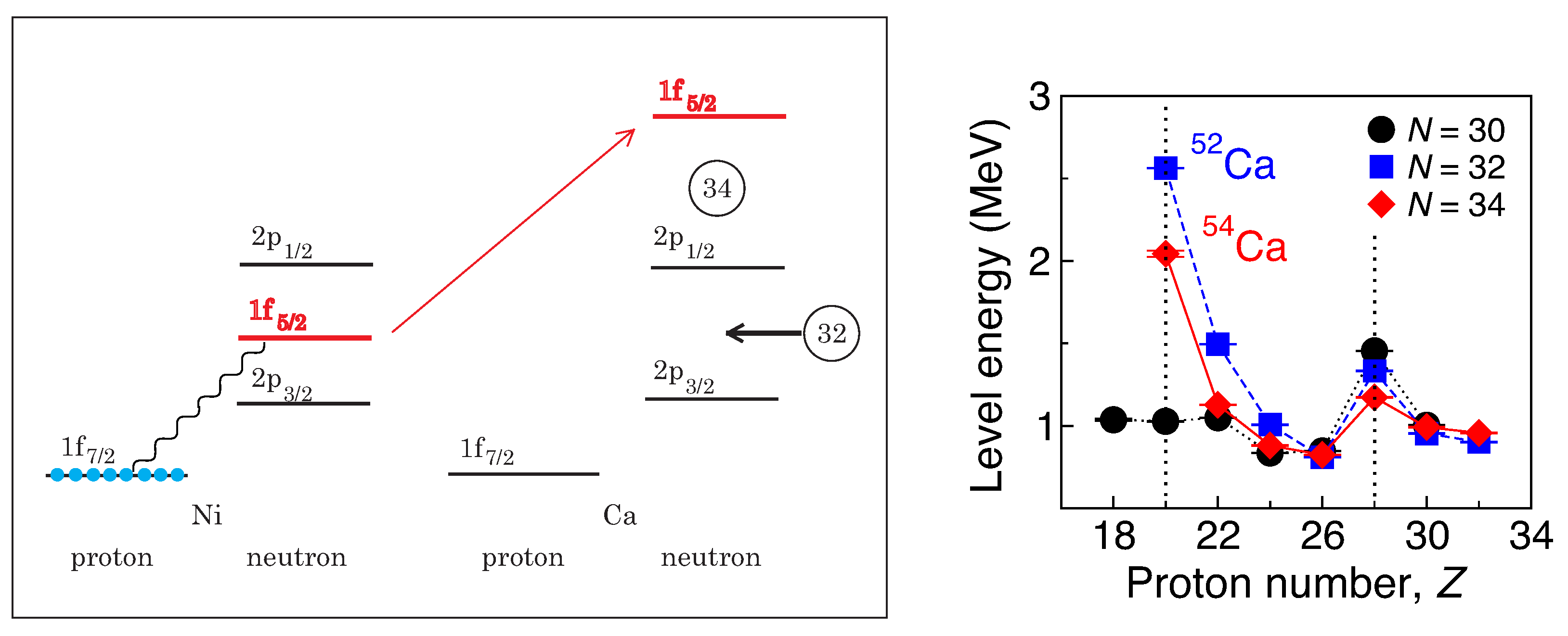
Among various cases of shell evolution, a notable impact was made by predicting a new magic number N = 34. Figure 7 displays the shell evolution of some neutron orbits from Ni back to Ca isotopes, as Z decreases from 28 to 20. The 1 orbit is between the 2 and 2 in Mayer–Jensen’s shell model (see Figure 1). By loosing eight protons lying in the 1 orbit of Ni isotopes (blue circles in Figure 7 left), this canonical shell structure is destroyed as the 1 orbit moves up above the 2 orbit. This movement of 1 orbit creates the N = 32 gap as a byproduct [44]. The energy shift in the 1 orbit is due to the central and tensor forces by almost equal amounts. We mention that the N = 34 magic gap would not appear, if the Mayer–Jensen scheme holds, as expected, in Ni isotopes but this shift did not occur. The appearance of the N = 34 magic number was predicted as a result of a spin–isospin interaction in [45]. However, 12 years were required [46] until the experimental verification became feasible [47] (see Figure 7 right). The measured 2+ energy levels are included in Figure 2b. More details are presented in [15]. Further evidences have been obtained recently by different experimental probes as reported in [48,49].
2.8. Monopole Interaction of the Two-Body Spin-Orbit Force
It is a natural question what effect can be expected from the two-body spin-orbit force of the interaction. This force can be well described by the M3Y interaction, and the monopole effects of the two-body spin-orbit force were described in detail in [15], particularly in its supplementary document. Although the monopole effects of this force contributes to the spin-orbit splitting [15], the effect is much weaker than the tensor force in most cases, as also discussed in the article by Utsuno in this volume.
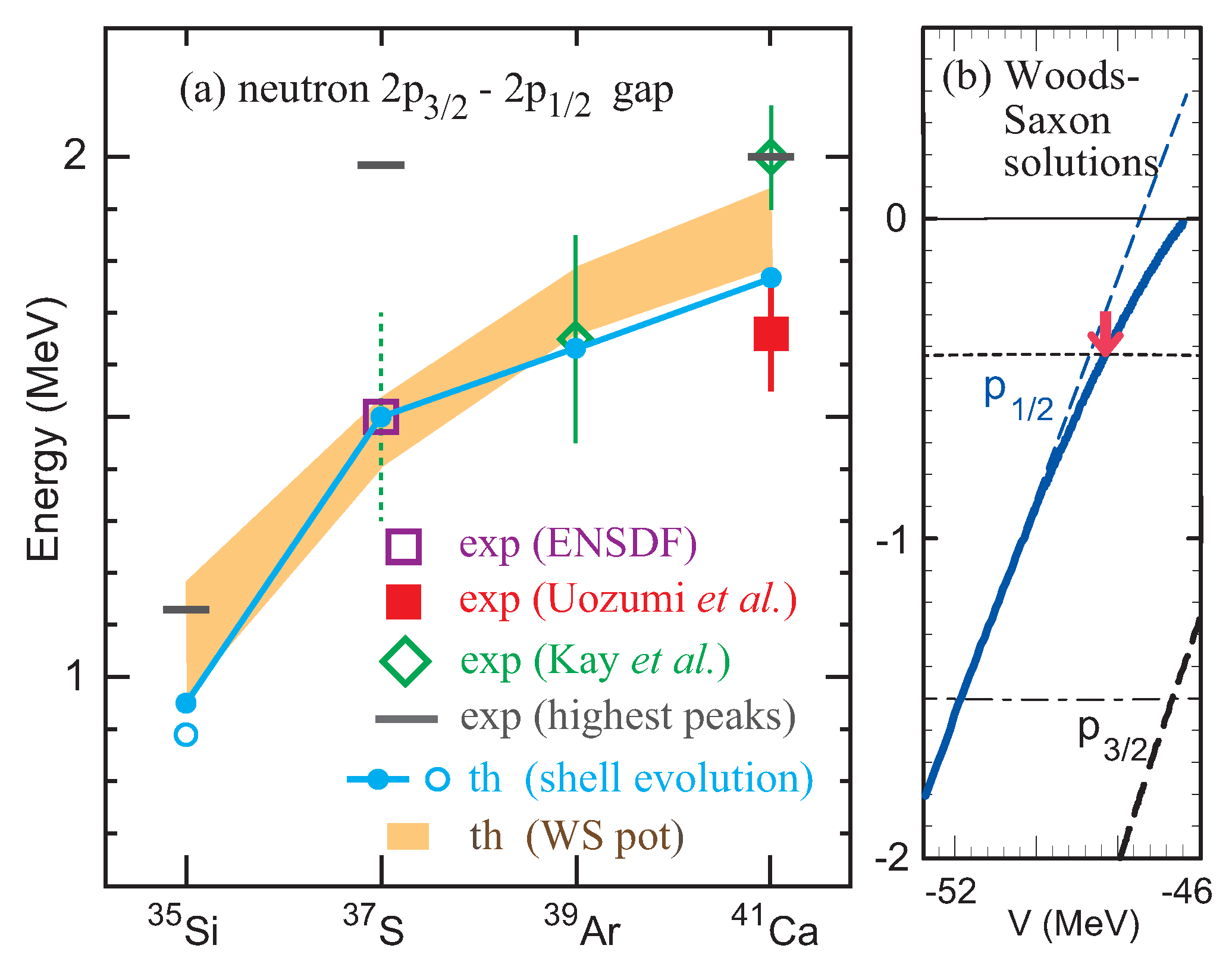
An interesting case is found in the coupling between an s orbit and orbits. There is no monopole effect from the tensor force, if an s orbit is involved. Instead, the s-p coupling due to the two-body spin-orbit force can be exceptionally strong as intuitively stressed in [15]. Figure 8 shows that the possible significant change in the neutron 2-2 gap between 35Si and 37S is explained to a good extent by the shell evolution due to the two-body spin-orbit force.
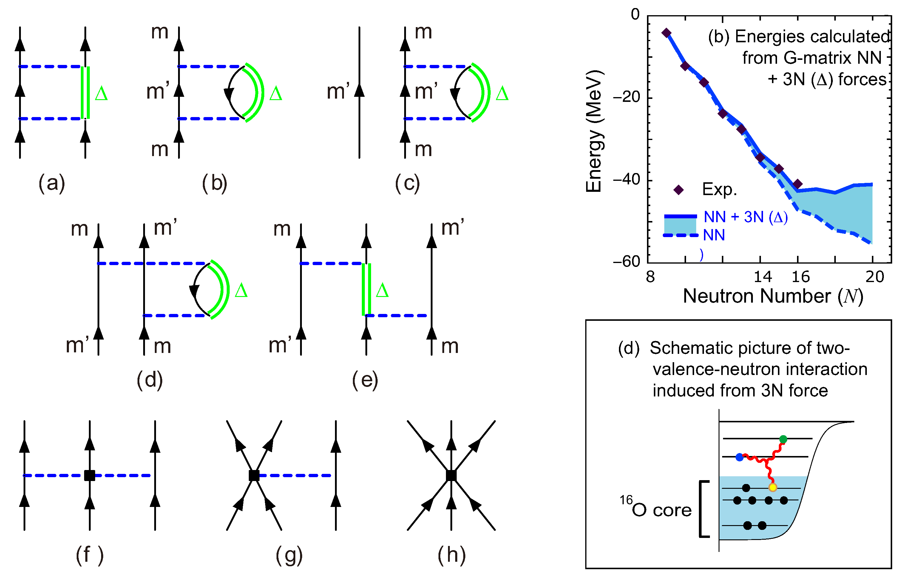
2.9. Monopole Interaction from the Three-Nucleon Force
The three-nucleon force (3NF) is currently of intense interest (see, for instance, a review [53]). Among various aspects, we showed [54] the characteristic feature of the monopole interaction of the effective interaction derived from the Fujita–Miyazawa 3NF [55]. Figure 9a displays the effect of the excitation in nucleon–nucleon interaction. The -hole excitation from the inert core changes the SPE of the orbit j as shown in Figure 9b, where m is one of the magnetic substates of the orbit j, and means any state. This diagram renormalizes the SPE, and observed SPE should include this contribution. If there is a valence nucleon in the state as in Figure 9c, the process in Figure 9b is Pauli-forbidden. However, in the shell–model and other nuclear-structure calculations, the SPE containing the effect of Figure 9b is used. One has to somehow incorporate the Pauli effect of Figure 9c, and a solution is the introduction of the process in Figure 9d. In this process, the state doubly appears in the intermediate state, but one can evaluate the Pauli effect by including Figure 9b,d consistently. This is a usual mathematical trick and enables us to correctly treat the Pauli principle within the simple framework. Figure 9d is equivalent to Figure 9e, which is nothing but the Fujita–Miyazawa 3NF, where the state appears in double. Similar treatment is carried out in the chiral Effective Field Theory (EFT) framework. Figure 9f corresponds to Figure 9e, but the violation of the Pauli principle is slightly hidden, because of a vertex in the middle (depicted by a square) instead of the -hole excitation.
In this argument, the 3NF produces a repulsive monopole interaction in the valence space, after the summation over the hole states of the inert core (see Figure 9 bottom right), which corresponds to the normal ordering in other works.
The plot Figure 9 top right indicates an example of the repulsive effect on the ground-state energy of oxygen isotopes, locating the oxygen dripline at the right place or solving the oxygen anomaly [54]. This is rather strong repulsive monopole interaction, which is a consequence of the inert core. This means that the present case is irrelevant to the no-core shell model or other many-body approaches without the inert core (e.g., Green’s Function Monte Carlo calculation [56]). This feature has caused some confusions in the past, but the difference is clear. The present repulsive monopole effect is much stronger than the other effects of the 3NF [57], and the latter will be better clarified by further developments of the chiral EFT for 3NF in the future. I note that the repulsive T = 1 effect was empirically noticed by Talmi in the 1960s [3].
2.10. Short Summary of This Section
The shell evolution phenomena are seen in many isotopic and isotonic chains and sometimes result in the formation of new magic gaps or the vanishing of old ones. Figure 2b displays the emergence of such new magic numbers N = 16, 32, and 34, whereas the lowering of some 2+ levels can mean the weakening of some magic numbers. More changes may appear in the future studies. Thus, the characteristic monopole features of the central, tensor, two-body , and 3NF-based interactions and the resulting shell evolution are among the emerging concepts of the nuclear structure. Interestingly, these findings are neither isolated nor limited to particular aspects but are related to other aspects of the nuclear structure. We now move on to such a case.
3. Type-II Shell Evolution and Shape Coexistence
3.1. Type-II Shell Evolution
The shell evolution shown in Figure 5b,c are due to the addition of two or four neutrons into the orbit , respectively. Instead of adding, one can put neutrons into the orbit by taking the neutrons from some orbits below , or equivalently by creating holes there, as shown in Figure 5d. If such a lower orbit happens to be the orbit as in Figure 5d, its monopole matrix elements show just the opposite trends compared to the orbit. However, because holes are created in , the sign of the monopole-interaction effect is reversed, and the final effect has the same sign as the monopole effect form the orbit (see Figure 5d). Thus, the particle–hole (ph) excitation of the two neutrons Figure 5d reduces the proton - splitting even more than in Figure 5b. This reduction becomes stronger with the ph excitations of four neutrons, as depicted in panel Figure 5e. Such strong reduction in the spin-orbit splitting produces interesting consequences beyond shell-structure changes. This type of the shell-structure change within the same nucleus is called type-II shell evolution.
3.2. A Doubly-Closed Nucleus 68Ni
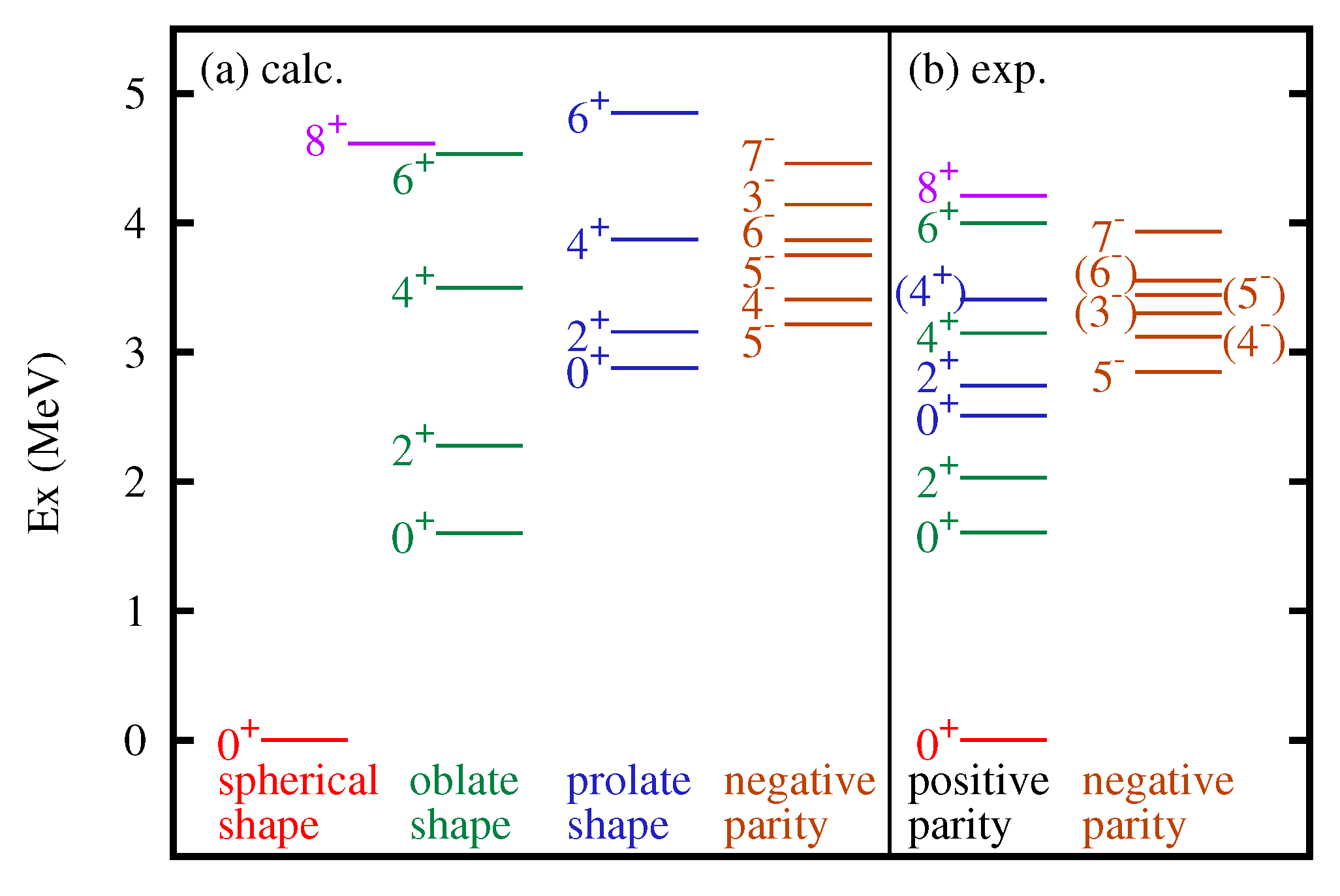
The Type-II shell evolution was first discussed in [58] for 68Ni as an example. Figure 10 shows its theoretical and experimental energy levels. The theoretical results were obtained for the A3DA-m interaction by the MCSM [59,60,61,62], which is a powerful methodology for the shell model calculation but is not discussed in this article due to the length limitation.
Because Z = 28 is an SO magic number and N = 40 is an HO magic number (see Figure 1), the ground state of 68Ni is primarily a doubly closed shell. Indeed, in the theoretical ground state, the occupation of the neutron orbit is negligibly small. In contrast, the state located at the excitation energy, Ex∼3 MeV, is the band head of a rotational band of an ellipsoidal shape, and its neutron occupation number is as large as ∼4. The mechanism shown in Figure 5e is then switched on, reducing the proton – splitting. A reduced splitting facilitates more configuration mixing between these two orbits, which can produce notable effects on the quadrupole deformation as stated below.
3.3. Coexistence between Spherical and Deformed Shapes
We here quickly overview the quadrupole deformation or the shape deformation from a sphere to an ellipsoid [13]. The quadrupole deformation is driven by the quadrupole interaction, a part of the multipole interaction in Equation (11). The quadrupole interaction is a somewhat vague idea because of a certain mathematical complication, but its main effects can be simulated by the (scalar) coupling of the quadrupole moment operators. If the quadrupole moments are larger, i.e., a stronger quadrupole deformation occurs, the nucleus gains more binding energy from the quadrupole interaction. This is a very general phenomenon, and because of this the ground states of many nuclei are deformed, although 68Ni is not among them.
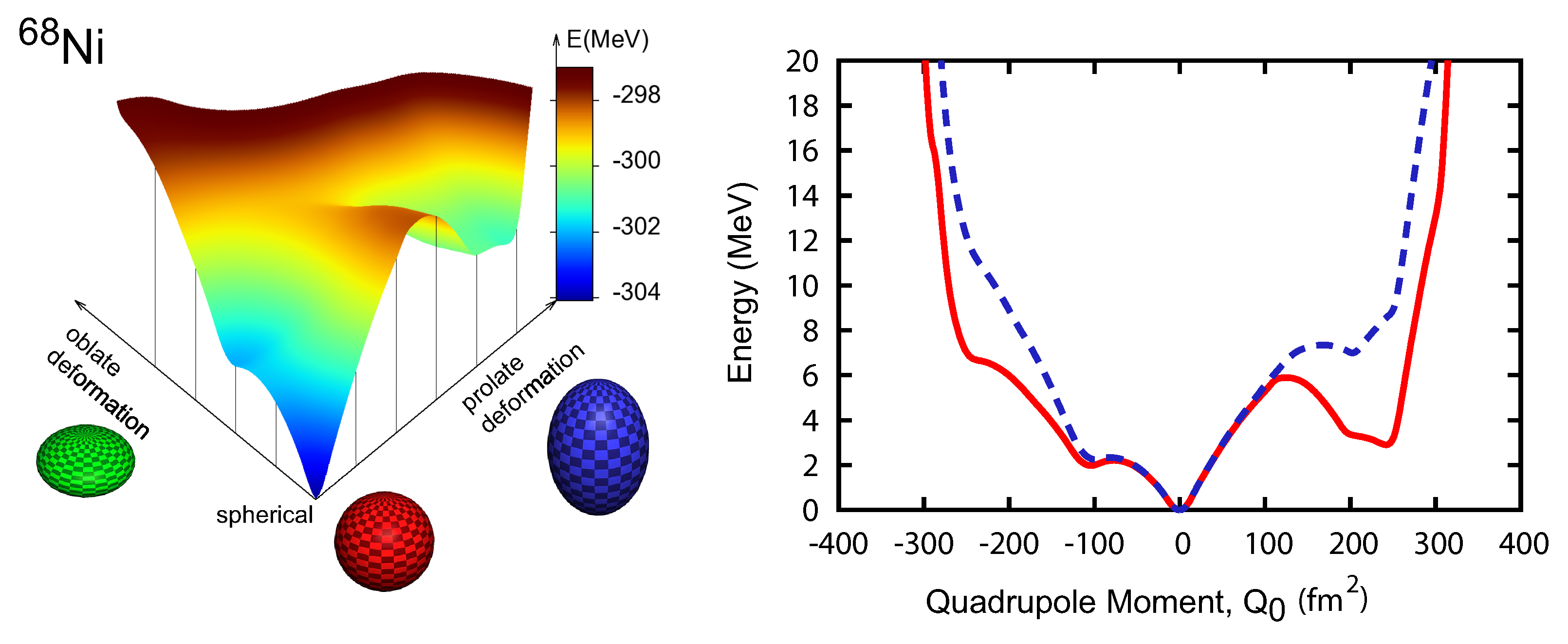
The energy of 68Ni (intrinsic state) is graphically illustrated in Figure 11 left for various ellipsoidal shapes, spherical, prolate, oblate and in between (called triaxial). The energy is calculated by the constraint Hartree–Fock (CHF) calculation with the same shell–model Hamiltonian as in Figure 10. The imposed constraints are given by the quadrupole moments in the intrinsic (body-fixed) frame, represented usually by and [13]. This plot is usually called the Potential Energy Surface (PES). The minimum energy occurs at the spherical shape (red sphere), with = = 0. The constraints are changed to a more prolate deformed ellipsoid (blue object) along the upper-right axis (“prolate deformation” in the figure), where increases but = 0. (Between two axes in Figure 11, . We come back to this point below.) The energy relative to the minimum energy climbs up by 6 MeV first. This is because protons and neutrons must be excited across the magic gaps from the doubly closed shell in order to create states of deformed shapes (see Figure 1). The energy then starts to come down, as the quadrupole moments increase, thanks to the quadrupole interaction. It is lowered by 3 MeV from the local peak to the local minimum. Beyond the local-minimum area, the effect of the quadrupole interaction is saturated, and it cannot compete with the energy needed for exciting more protons and neutrons across the gaps required by the constraints. This energy variation appears as the basin in the three-dimensional PES. This is the usual explanation of the local deformed minimum. The appearance of two (or more) different shapes with a rather small energy difference is one of the phenomena frequently seen and is called the shape coexistence [63]. The quadrupole interaction is undoubtedly among the essential factors of the shape coexistence. However, this may not be a full story.
Figure 11 right exhibits the same energy along the axis lines of Figure 11 left, where is varied from −400 fm2 to 400 fm2 while = 0 is kept. The positive (intrinsic) quadrupole moments ( > 0) imply prolate shapes (blue object in Figure 11 left), whereas the negative ones imply ( < 0) oblate shapes (green object). The red solid line shows the CHF results of the full Hamiltonian, whereas for the dashed line, the tensor monopole interactions between the neutron orbit and the proton orbits are practically removed. This removal means no effects depicted in Figure 5d,e. The dashed line displays a less-pronounced prolate local minimum at weaker deformation with much higher excitation energy. The significant difference between the solid and dashed lines suggests that the monopole effects are crucial to lower this local minimum and stabilize it. We now discuss the mechanism for this difference. With the tensor monopole interaction, once sufficient neutrons are in , the proton – splitting is reduced, and this reduced splitting facilitates the mixing between these two orbits driven by the quadrupole interaction. The resulting deformation is stronger compared to no tensor-force case. In parallel to this, the tensor monopole interaction involving the neutron orbit produces extra binding energy, if more protons are in and less are in . This extra binding energy lowers the deformed states, otherwise they are high in energy because of the energy cost for promoting neutrons from the shell to . Thus, a strong interplay emerges between the monopole interaction and the quadrupole interaction, and type-II shell evolution materializes this interplay in the present case. It enhances the deformation and lowers the energy of deformed states. Without this interplay, as indicated by blue dashed line in Figure 11 right, the rotational band corresponding to the local minimum is pushed up by 4 MeV and may be dissolved into the sea of many other states. It is obvious that this interplay mechanism works self-consistently.
3.4. T-Plot Analysis
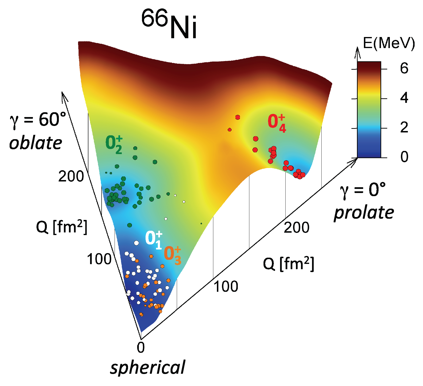
The T-plot was introduced in the same Ref. [58], in order to clarify what shapes are more relevant to individual eigenstates of the shell–model calculation. Let us take an example. Figure 12 [64] depicts the PES of 66Ni with the same Hamiltonian as in Figure 10. The small circles on the PES are the T-plot. The T-plot is obtained from MCSM eigenstate. We therefore briefly explain the MCSM eigenstate. An MCSM eigenstate, , is written, with the ortho-normalization, as
where denotes amplitude; means the projection operator on to the spin/parity (this part is more complicated in practice); and stands for a Slater determinant called (k-th) MCSM basis vector: = . Here, is the inert core (closed shell); refers to a superposition of usual single-particle states,
with being the creation operator of a usual single-particle state, for instance, that of the HO potential, and denoting a matrix element. By choosing an optimum matrix , we can select so that such better contributes to the lowering of the corresponding energy eigenvalue. Thus, the determination of is the core of the MCSM calculation. The index k runs up to 50–100 but sometimes to 300 at maximum. These are much smaller than the dimension of the many-body Hilbert space.
Each has intrinsic quadrupole moments ( and ), where imply the operators for mentioned above. The T-plot circle for is placed according to those values on the PES with its area proportional to the overlap probability with the corresponding eigenstate, i.e., in Equation (16). Such T-plot circles are shown in Figure 12. The white circles represent the MCSM basis vectors for the ground state, while the red circles indicate the MCSM basis vectors for the state, which is strongly deformed. Although there is no local minimum for oblate shape, the state is shown to be moderately oblate deformed. The T-plot can thus give partial labeling to fully correlated eigenstates for mean values as well as fluctuations with respect to their quadrupole shapes. The advantages of mean-field approaches are now nicely incorporated into the shell model.
3.5. Short Summary of This Section
Type-II shell evolution occurs in various cases, especially in a number of shape coexistence cases, providing deformed states with stronger deformation, lower excitation energies, and more stabilities. It is an appearance of the monopole–quadrupole interplay and plays crucial roles in various phenomena including the first-order quantum phase transition (Zr isotopes [65,66,67]), the second-order quantum phase transition (Sn isotopes [68]), the multiple even-odd quantum phase transitions (Hg isotopes [69]), as well as the raising of the intruder band due to the suppression of the type-II shell evolution (lighter Ni isotopes [64,70]). As the involvement of the monopole interaction in this manner had not been recognized, type-II shell evolution appears to be among the emerging concepts of nuclear structure. The type-II shell evolution has been clarified by the T-plot in many cases. Including other contributions, the T-plot is undoubtedly one of the emerging concepts of nuclear structure, apart from its impact on the computational methodology.
4. Self-Organization and Collective Bands in Heavy Nuclei
We now proceed to more general cases of the monopole–quadrupole interplay. This interplay leads to unexpected consequences in the underlying mechanism of collective bands of heavy nuclei [71], beyond the standard textbooks.
The MCSM has become powerful enough [62] to reproduce collective bands of heavy nuclei such as 154Sm and 166Er, with one and half HO major shells [71]. We sketch the new findings by using the results of such most-advanced MCSM calculations.
4.1. Shape Coexistence in 154Sm
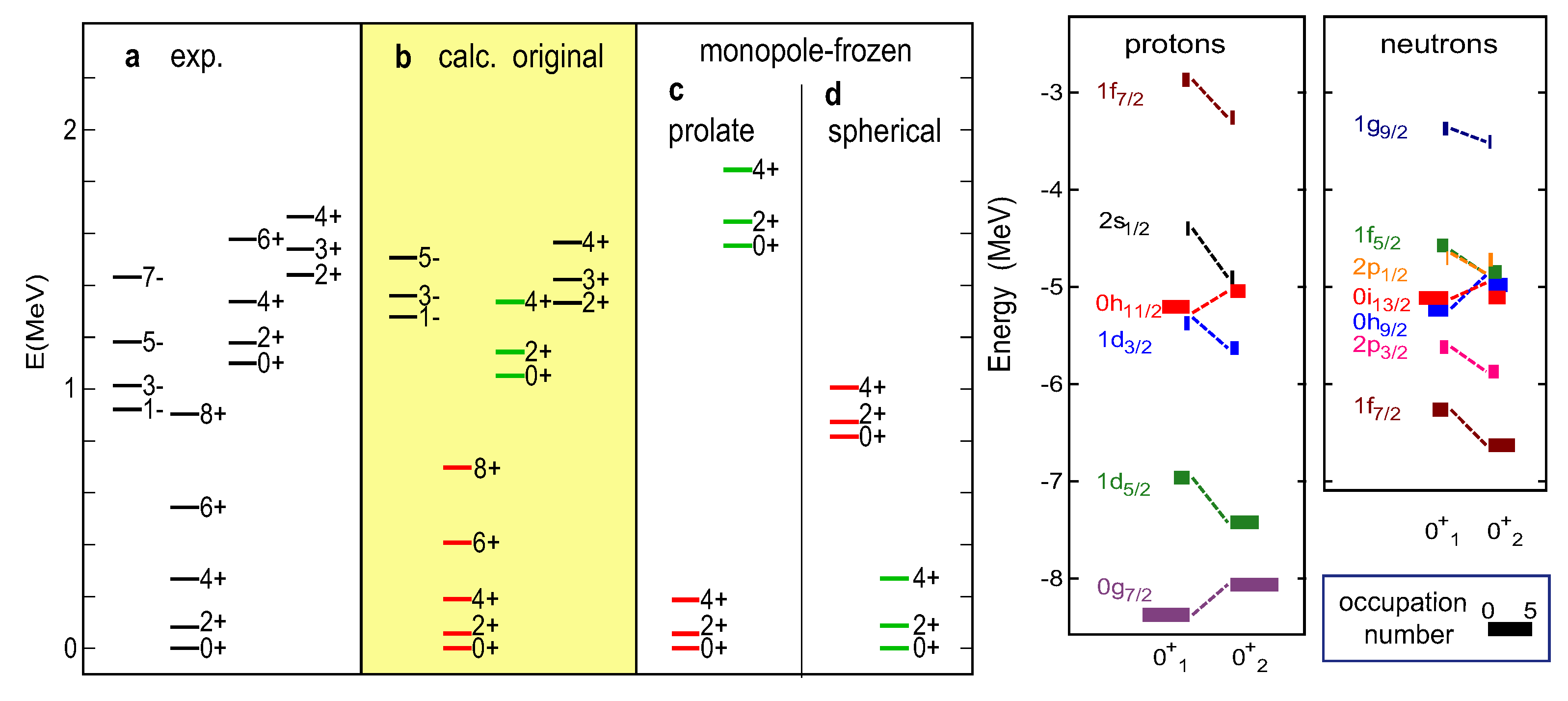
Figure 13 shows low-lying energy levels of 154Sm. The present MCSM calculation can describe the four low-lying bands including the negative-parity one. The agreement between the experimental levels in Figure 13a and the theoretical levels in Figure 13b is rather good. Although the importance of the quadrupole interaction is evident for the formation of deformed rotational bands, one can investigate to what extent the monopole interaction is involved. The monopole interaction here was obtained from the shell–model interactions, comprising the central, tensor, and other components.
The monopole interaction is an operator, but we “freeze” it now: its ESPE expectation values are calculated for the state to be specified, and the obtained values are adopted as the SPEs, in Equation (4), with the monopole interaction removed. We then perform the shell-model calculation and draw the PES. This toy game is called the “monopole-frozen” analysis [71], as the monopole properties are included only through the specified state. Figure 13c exhibits the energy levels obtained by the monopole-frozen analysis referring to the ground state. The band built on the state (often called the band) is lifted up by 0.5 MeV (∼50% of the original excitation energy), suggesting that the active monopole interaction produces a substantial lowering of this state. Figure 13d shows the monopole-frozen analysis referring to the spherical HF state: the ground state is no longer prolate, but triaxial, with the wave function close to the state of the original Hamiltonian. Thus, the crucial effect of the monopole interaction is verified.
Figure 13 right shows the actual values of for the and states. This figure demonstrates the significant differences between two sets of the ESPE values. The occupation numbers are also different: there are more half-filled orbits for the state, which is indicative of its triaxial nature. The smaller occupation numbers of unique-parity orbits are also consistent with the tendency away from the prolate shape.
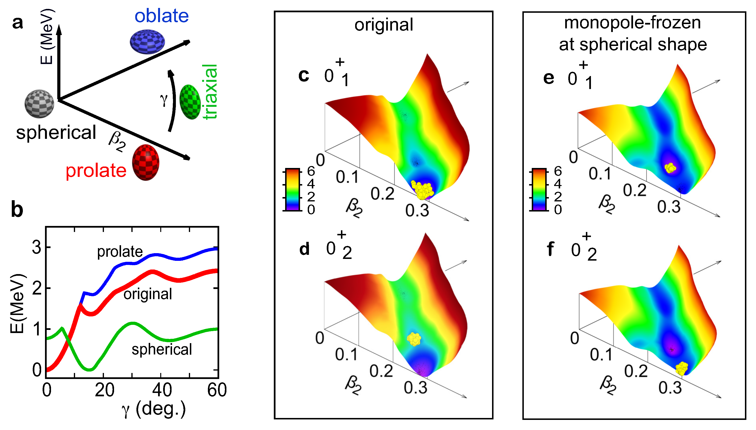
We now introduce the deformation parameters and [13], and their meanings are sketched in Figure 14a. The parameter represents the magnitude of the ellipsoidal deformation from sphere. The ellipsoid has three axes: the longest, middle, and shortest. The parameter is an angle between and and represents mutual relations among the lengths of these axes: = means that the middle and shortest axes have the same length (prolate); = implies that the longest and the middle ones have the same length (oblate); and values in between stand for intermediate situations, called triaxial. Figure 11 and Figure 12 include them. The and parameters can be obtained, in some approximation, from intrinsic quadrupole moments through the formulas [72],
and
where e is the unit charge; () denotes proton (neutron) effective charge induced by in-medium (or core-polarization) effects; and stands for the radius parameter of the droplet model (spherical background) (see [73] for some detailed explanation). The relations in Equations (18) and (19) worked very well in many works, for instance [64,69,70,71].
Figure 14c,d shows the T-plot for the original interaction, where the PES is shown by using and as coordinates (see Figure 14a). Figure 14e,f depicts the T-plot for the monopole-frozen interaction obtained with the spherical HF state. The T-plot patterns are consistent with the above features suggested by the shell–model diagonalization. The cut of the PES shown in Figure 14b suggests that the local minimum is raised by the monopole-frozen process referring to the ground state.
Figure 14c,d depict a valley of the PES with a local minimum around . Similar valleys are seen in the PES obtained by the mean-field calculations [74,75], implying that this valley likely has a common origin. On the other hand, one can state that the present monopole effect results in not only the valley but also the local minimum, and the latter plays essential roles in the formation and stability of the side bands. It is of interest to refine the monopole interaction in mean-field models.
Regarding the vibration picture of the state, the present view is opposed to such a conventional view. The triaxial deformation is shared by the members not only of the band but also of the band (usually called band), as can be verified by their T-plots. Namely, the state is the “ground” state of the triaxial states to which both the and bands belong. In short, this is a shape coexistence between the prolate and triaxial shapes assisted by the interplay between the monopole interaction and the quadrupole deformation. It is noted that the vibration picture of the states has been investigated from experimental viewpoints [76,77].
4.2. Collective Bands and Vibration in 166Er
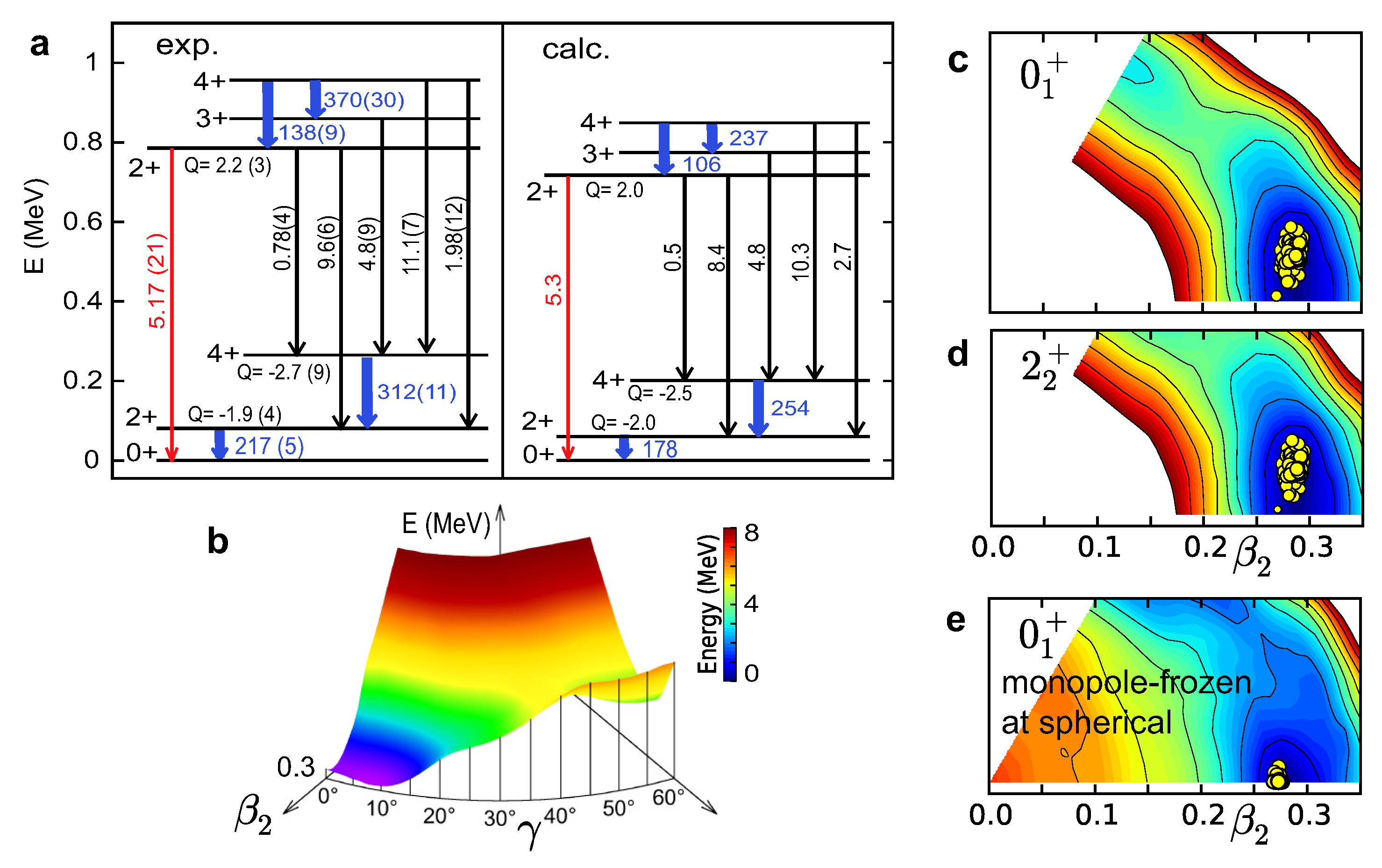
The features of the collective motion in 166Er have been studied by the MCSM similarly well (see Figure 15a). Among rotational nuclei, 166Er is characterized by particularly low-lying state and the band built on it. Aage Bohr stressed that this state was a vibration from the prolate ground state [9,10,11,13]. The relatively strong → E2 transition (B(E2)∼5 W.u., see Figure 15a, was ascribed to the annihilation of one phonon in the state. This was one of the major points of the Nobel lecture by Aage Bohr and has been a common sense as stated in many textbooks of nuclear physics. We now challenge this traditional belief, by utilizing the recent MCSM calculation. It is reminded that no firm experimental evidence to uniquely pin down the -vibration nature of 166Er has been reported and also that in a systematic calculation of many heavy nuclei [78], the excitation energies of the states in the band appeared to be about twice higher than the observed values, despite much better description of those of the state in the ground band.
Figure 15b shows the calculated PES, which shows the minimum not at but around (see also [80]). The T-plot is shown for the and states in Figure 15c and Figure 15d, respectively. The patterns of the T-plot circles are nearly identical between these two panels. This is consistent with a (rigid) triaxial interpretation, and indeed E2 transition strengths follow the predictions of the Davydov triaxial model [81,82] with . Certainly, a pure rigid triaxiality is not the correct picture, and there are quantum fluctuations, as evident from Figure 15c,d [80]. After all, the displacement from the is obvious. The triaxiality of 166Er is also suggested by the triaxial projected shell model, although the rigid-triaxiality is not an outcome but an assumption [83,84].
The experimentally known = 4 state around 2 MeV excitation energy provides a long-standing puzzle [85,86]: the observed relatively strong E2 transition from this state to the state looks like a sign that the state and this = states are the single- and double-phonon states in the vibration picture (à la A. Bohr [9,10]), respectively, but the excitation energy of this = state is too high for a double-phonon excitation. The present calculation, on the other hand, reproduces both the excitation energy and the E2 transition strength, and this = state appears as the = member of the triaxial states including the and states (see Figure 15c,d) [71,80]. Thus, the triaxiality is shown to be one of the key aspects for understanding/predicting the shapes of heavy nuclei.
The monopole-frozen analysis referring to the spherical CHF state shows that the ground state moves to , confirming the important role of the monopole interaction activated. The triaxial ground states are now shown to appear in a large number of nuclei in the nuclear chart, besides the known triaxial domain [87].
4.3. A Historical Touch and a Short Summary of This Section
The collective bands in heavy nuclei have traditionally been understood in terms of the ground band with axially symmetric prolate shape and the side bands with the or vibrational excitations from the ground state. This picture is consistent with the Nilsson model [88] and was confirmed by the Pairing + Quadrupole-Quadrupole (P+QQ) model [89,90], where the monopole interaction is not included, however. It has been shown in this section that the monopole interaction is crucial also for the collective bands in heavy nuclei. We just note that in lighter nuclei, the situation can be different mainly because of small model spaces comprising single or a few active orbits, where the rotational motion has been nicely described by symmetry-based approaches, e.g., SU(3) model of Elliott for the shell [91,92], and by realistic calculations, e.g., on 48Cr [93].
Regarding heavy nuclei, for individual rotational bands, the monopole interaction contributes differently, and the intrinsic structure is determined not only by the quadrupole interaction but also by the monopole interaction, as verified by the monopole-frozen analyses. Thus, the monopole–quadrupole interplay arises. The monopole interaction does not directly drive the deformation but optimizes the ESPEs so that more binding energy is gained. This gain is state-dependent and even can alter the ordering of bands as mentioned above. The present monopole–quadrupole interplay can be described also from the viewpoint of the self-organization [71]: the nucleus is changed from a disorder (original SPEs) to an order (ESPEs tailored to the shape of interest) by activating the monopole interaction. As this occurs “purposely” towards certain shapes with positive feedback, particularly between the monopole and quadrupole effects, the whole picture fits well the (quantal) self-organization [71]. The self-organization for collective bands is among the emerging concepts of nuclear structure, showing novel consequences. For example, the dominant fraction of the ground states of heavy nuclei are expected to show triaxial shapes, as another emerging concept of nuclear structure, in contrast to the traditional view of the prolate shape dominance in those states.
Appendix B presents a possible extension or generalization of the current idea to “many-ingredient” systems outside nuclear physics.
5. Dripline Mechanism
5.1. Traditional View
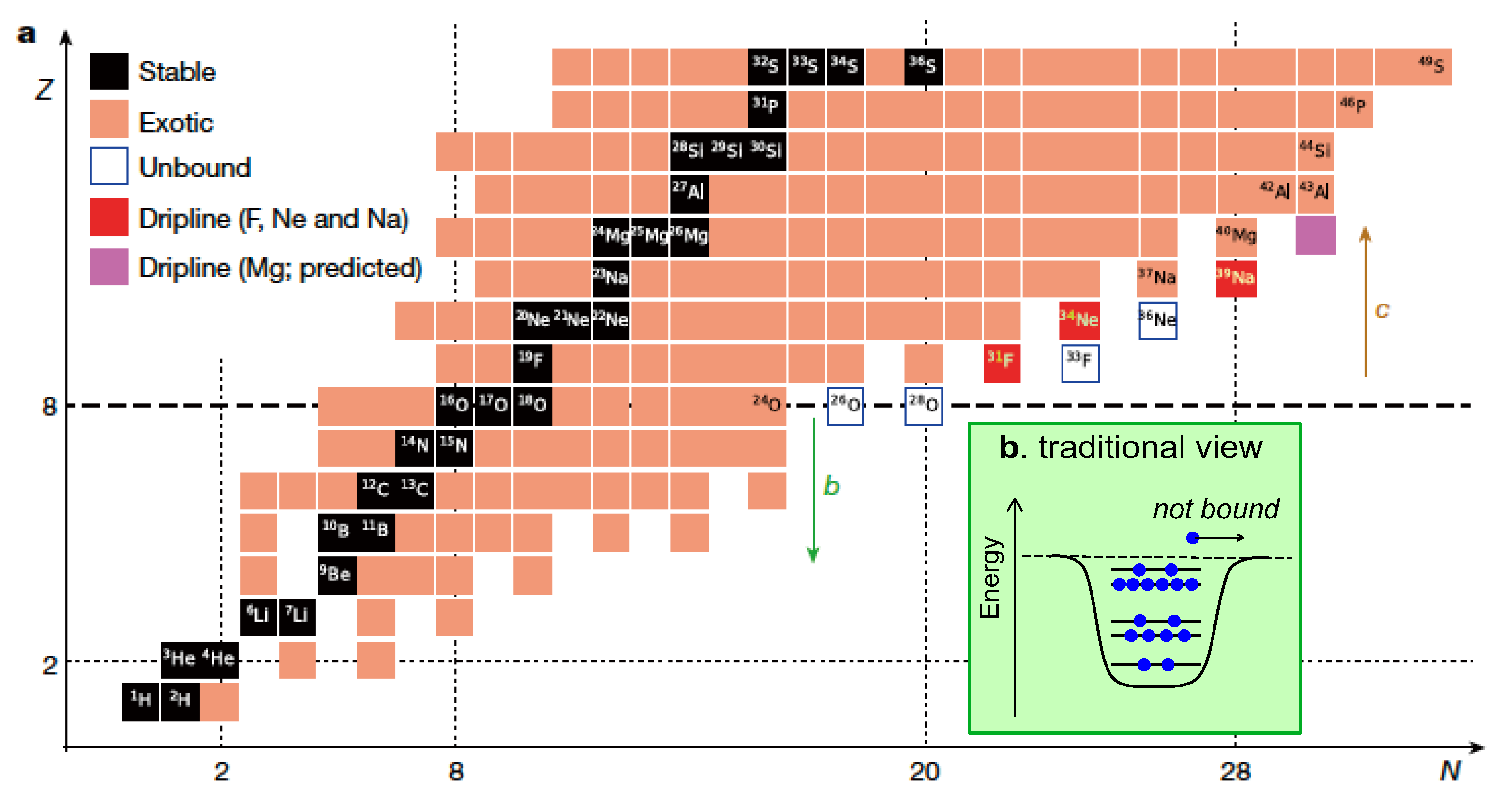
Figure 16a shows the left-lower part of the nuclear chart (Segrè chart) for . The black squares represent stable nuclei while the orange ones exotic nuclei (see Section 1). An isotopic chain is a horizontal belt, and its neutron-rich end is called neutron dripline. The location of the dripline in the nuclear chart implies the extent of the isotopes and is of fundamental importance to nuclear science. The experimental determination of the dripline is a very difficult task. Very recently, as shown by red squares in Figure 16a, the driplines of F and Ne isotopes and its candidate of Na isotope were reported [94].
The traditional view of the dripline is shown in Figure 16b: all bound single-particle orbits are occupied, and the next neutron goes away. It is an open question whether this view is valid for all nuclei or not. We look into this question now [57].
The structure of neutron-rich exotic isotopes of F, Ne, Na, and Mg can be well described by the shell–model calculation with the full + shells and the EEdf1 interaction [95]. This interaction was derived from the chiral EFT interaction of Machleidt and Entem [96], first processed by the method [97,98] and then processed by the EKK (Extended Krenciglowa-Kuo) method [99,100,101]. The method is used to transform the nuclear forces in the free space into a tractable form for further treatments. The method has been adopted for the derivation of other modern shell–model interactions, for instance, the one by Coraggio et al. for Sn and Cr-Fe regions [102,103].
The present work is unique in the usage of the EKK method, which enlarges the scope of the approaches based on the many-body perturbation theory (MBPT) [29]. The MBPT produced the G-matrix interactions in its early formulations [28], from which many useful shell–model interactions have been constructed (see Section 2.6). However, the resulting G-matrix interaction shows a limitation that if two major shells are merged, the results may diverge [101]. As the gap between two shells often vanishes or becomes smaller in exotic nuclei, this difficulty can be fatal there, although it is irrelevant to one-major-shell calculations. The EKK method nicely avoids this difficulty besides other merits.
Here, I present a very quick sketch of the formal aspect of the EKK method focusing on the logical flow based on Refs. [99,100,101] particularly the last one. This paragraph is not so relevant for understanding later parts of the article and can be skipped. In this paragraph, the symbol for operators is omitted for clarity. The EKK method starts from the separation of the Hamiltonian H with a parameter as
where P stands for the projection onto the Hilbert space explicitly treated (called P space usually), and . From this equation, we obtain the effective Hamiltonian for the P space at the n-th stage of the successive process,
where means for any operator O, e.g., . Here, the Bloch–Horowitz Hamiltonian is written as,
wherethe second term on the r.h.s. is called the Q-box. The quantity in Equation (21) represents its k-th derivative with respect to . Provided that is achieved, we can regard and use them as the effective Hamiltonian, . The effective interaction, like the EEdf1 interaction, is obtained as with being the unperturbed Hamiltonian (usually the SPEs). The solution of the given many-body problem remains (almost) unchanged within a certain range of . In fact, the parameter can be interpreted as the origin point of a Tayler expansion in a generalized sense. The divergence due to the energy denominator does not occur if the adopted values are far from the poles causing the divergence. I would like to stress that by construction, this effective Hamiltonian produces the exact solutions, once the convergence is achieved. This sketch is expected to depict that the EKK method is an expansion but not a perturbation one. This can be exemplified by the feature that the final result is independent of the parameter, in contrast to the perturbation expansion.
The EEdf1 interaction has thus been derived in an ab initio way by the and EKK methods from the chiral EFT interaction of Machleidt and Entem [96]. Some effects of 3NF are included in terms of the effective interaction by averaging over the hole states in the inert core, of which the monopole part is discussed in Section 2.9. While the Fujita–Miyazawa 3NF was used so far, other 3NF can be taken [57]. The EEdf1 interaction describes the properties of the ground and low-lying states of F, Ne, Na, and Mg isotopes quite well [57,95].
5.2. Monopole–Quadrupole Interplay for the Driplines
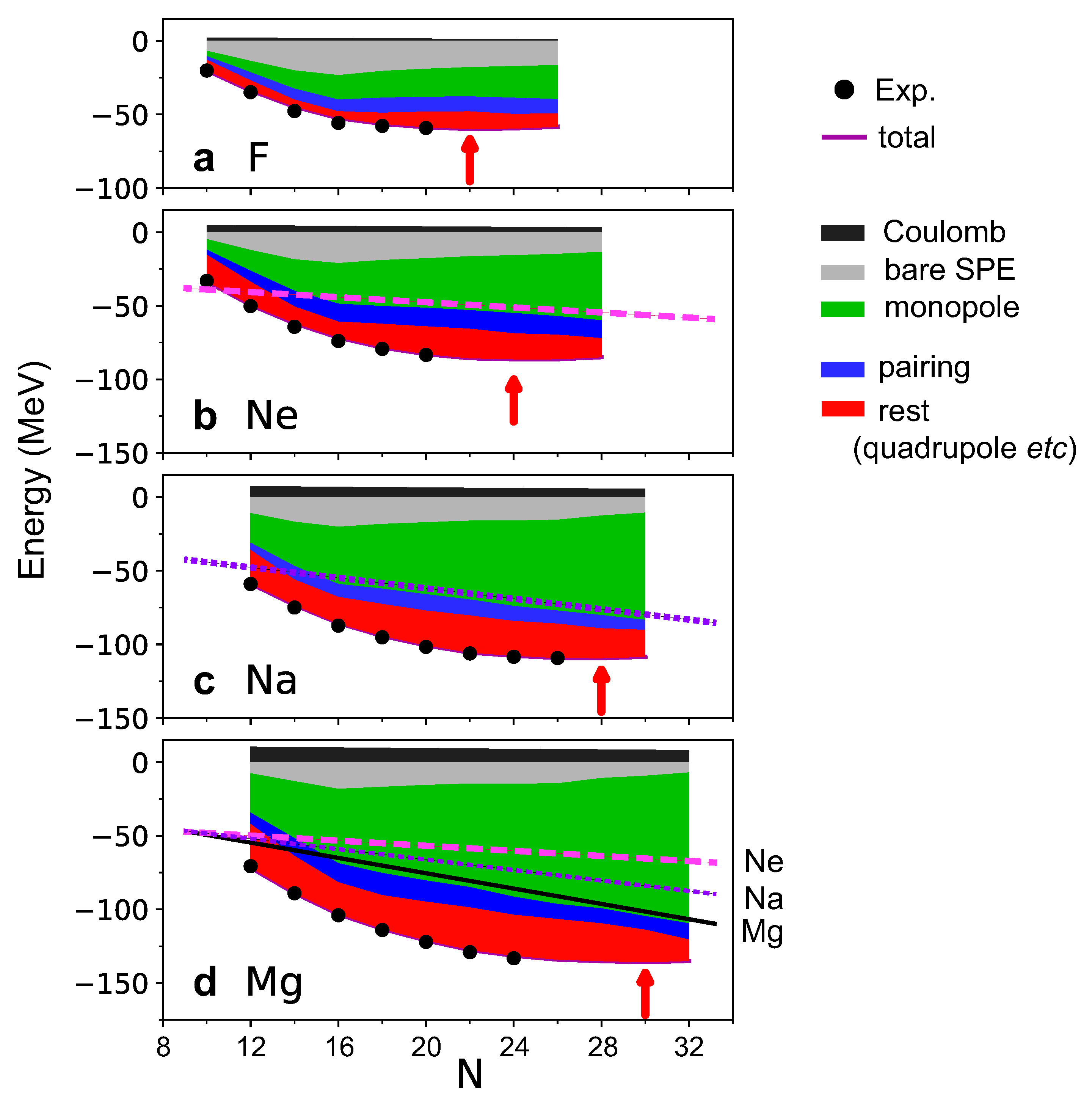
Figure 17 shows the ground-state energies of F, Ne, Na, and Mg isotopes as functions of the neutron number N. These energies are decomposed into several pieces according to their origins: SPE (on top of the 16O inert core), monopole, pairing, and rest terms. The Coulomb contribution is ignored in the following discussion, because it is of virtually no relevance. Here, the multipole interaction is divided into the pairing and rest terms. The pairing is the BCS-type pairing interaction acting on two neutrons coupled to and on two protons coupled to . The rest term means the multipole interaction subtracted by the pairing term. Although the rest term contains many different pieces, its major effects in the present discussion is simulated by the quadrupole interaction. This is the reason why the rest term is associated with “(quadrupole etc)” in the figure.
The lower edges of the red areas exhibit the ground-state energies as functions of the neutron number N, while only even N values are taken. These values show a good agreement with measured values shown by black dots. As long as the ground-state energy becomes lower as N increases, the isotope gains more binding energy by having more neutrons, and the isotope chain is stretched. However, if the ground-state energy is not lowered, there is no gain in the binding energy by having these extra neutrons; these extra neutrons are emitted, and the neutron dripline implies the nucleus with the lowest ground-state energy. The driplines obtained by the present calculation are shown by red arrows for each isotopic chain, reproducing experimental driplines for F, Ne, and Na isotopes [94].
We focus on the lower edge of the green areas in Figure 17. This represents the monopole contributions comprising the SPE and the monopole interaction. For Ne, Na, and Mg isotopes, this edge is lowered almost linearly as N increases from N = 16 to each dripline. We then fit the edge with pink dashed, purple dotted, and black solid lines for Ne, Na, and Mg isotopes, respectively. The lines of Ne and Na isotopes are copied to the panel for Mg, with their positions adjusted at a certain N. It is evident that the lines become steeper almost linearly as Z increases. This edge is almost flat for F isotopes for , and this feature is discussed below.
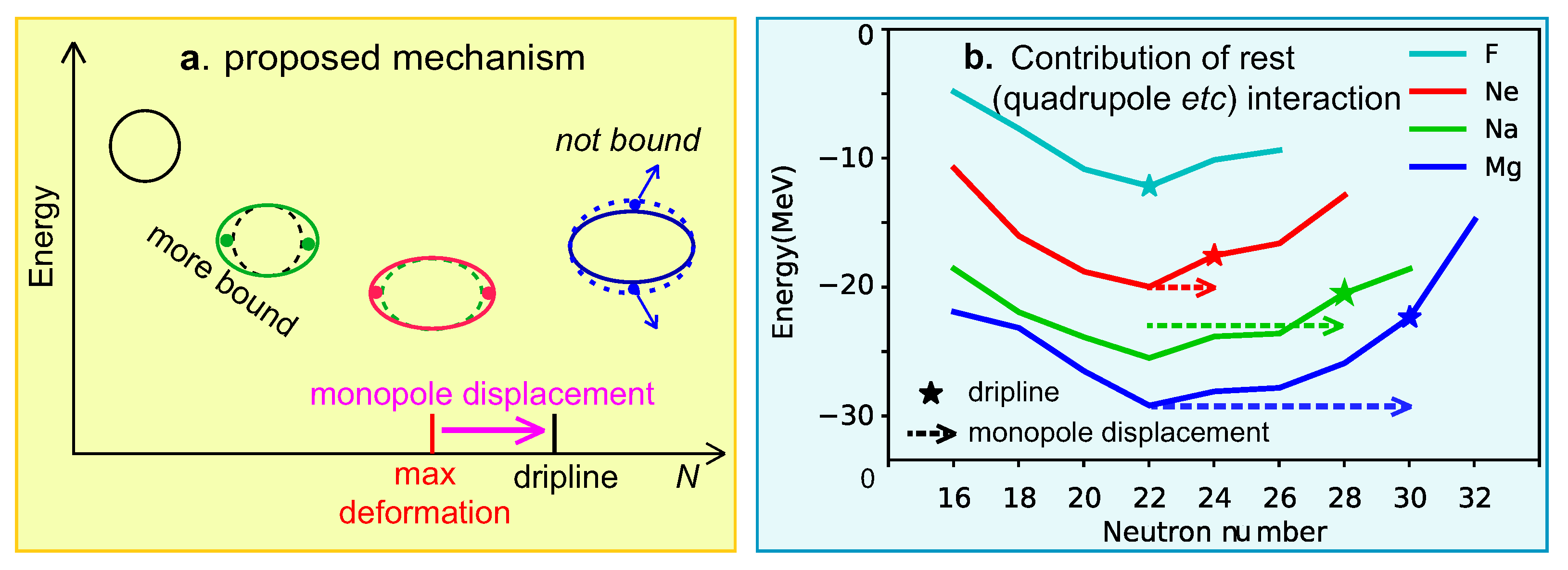
Figure 17 indicates that the effect of the pairing term shows small variations. In contrast, the rest term changes more, which is largely due to the quadrupole interaction. Figure 18a schematically indicates the variation of the effect of the quadrupole interaction: The effect is small at the far-left position with a spherical shape. As some neutrons are added, the shape is deformed, and the ground-state energy is lowered due to the quadrupole interaction. This trend continues but becomes its maximum at a certain value of N (red object in the figure). However, the dripline is not determined just by this maximum point.
Figure 18b depicts the actual effect of the rest term. It follows the trend illustrated in Figure 18a, with the maximum effect at N = 22 in all four chains. However, the driplines are different among these four. This is due to the monopole interaction. Let me explain it by taking the Mg isotopes as an example. The black straight line of the monopole effect in Figure 17d depicts about 3 MeV lowering per additional neutron, implying about 6 MeV for an additional two neutrons. After N = 22, the rest effect loses its magnitude. If the loss is less than the monopole gain (∼6 MeV), this loss is compensated by the monopole effect. However, the loss becomes larger for N larger, and at a certain point, the loss exceeds the monopole compensation. The dripline thus arises with the “monopole displacement” from N = 22 to N = 30 as shown in Figure 18b (and also in Figure 18a schematically).
The monopole effect depends directly on the number of protons, as visualized by three straight lines in Figure 17. Consequently, the monopole displacement is = 2 (6) for Ne (Na) isotopes. For F isotopes, the monopole effect is negligibly small for 16, and the dripline is located at the maximum rest (quadrupole etc.) effect.
5.3. Stability of Spherical Isotopes and the Monopole-Quadrupole Interplay
An immediate lemma of the present dripline mechanism is that the driplines of spherical nuclei, such as Ca, Sn, and Pb isotopes, can be further away from the stability line than other elements. One can assume a basically constant pairing contribution and a minor rest-term contribution. These two are thus irrelevant to the driplines of these isotopes. The remaining monopole effect gradually changes, pushing the driplines away.
5.4. A Short Summary of This Section
The present new dripline mechanism [57] involves the monopole–quadrupole interplay and is one of the emerging concepts. It definitely differs from the traditional mechanism of the single-particle origin, where a neutron halo arises at extremes [104,105]. In the new mechanism, the coupling to continuum may be visible if the monopole effect vanishes like heavy F isotopes [57]. As Z changes, two dripline mechanisms may appear alternatively, but the present one may be more relevant to heavier nuclei where the deformation develops more. Finally, I would like to point out that the Bethe–Weizäcker mass formula does not include a deformation energy term, at least, explicitly.
6. Prospect
As this article is a kind of summary, I am afraid that a summary section may be redundant. I state some prospects. First of all, ab initio no-core Monte Carlo shell–model calculations became feasible recently up to 12C and beyond [106], and as an example, we can look into clustering in light nuclei, e.g., the Hoyle state, with correlations produced by nuclear forces [107]. This direction will produce a major outcome from the shell model. This includes clarifications of decay, knockout, etc. Another major frontier is the quest for fission dynamics and superheavy elements, with (almost) full inclusion of the correlations due to nuclear forces.
Although more computer power and further advancements in computational methodology are needed also, the perspectives of the shell model look unlimited, to me. May the (nuclear) force be with you.
Funding
This work was supported in part by MEXT as “Program for Promoting Researches on the Super computer Fugaku” (Simulation for basic science: from fundamental laws of particles to creation of nuclei) and by JICFuS. This work was supported by JSPS KAKENHI Grant Numbers JP19H05145, JP21H00117.
Data Availability Statement
Not applicable.
Acknowledgments
The author is grateful to A. Gargano and S.M. Lenzi for their interests and for the invitation to this valuable program. He acknowledges T. Abe, Y. Akaishi, B.A. Brown, P. Van Duppen, B. Fornal, R. Fujimoto, A. Gade, H. Grawe, R.V.F. Janssens, M. H.-Jensen, K. Heyde, J. Holt, M. Honma, M. Huyse, Y. Ichikawa, S. Leoni, T. Mizusaki, N. Pietralla, P. Ring, E. Sahin, J. P. Schiffer, A. Schwenk, N. Shimizu, O. Sorlin, Y. Sun, T. Suzuki, K. Takayanagi, T. Togashi, K. Tsukiyama, N. Tsunoda, Y. Tsunoda, Y. Utsuno, S. Yoshida, and H. Ueno for their valuable direct collaborations towards the works presented in this article and thanks many others for their useful comments and help. The comment by Y. Tsunoda on Appendix A is appreciated.
Conflicts of Interest
The author declares no conflict of interest.
Appendix A. Note on the Relation between the Present ESPE and the Baranger’s ESPE
This is a short note on the the relation between the present ESPE and Baranger’s ESPE [19] discussed in [15]. A possible problem was pointed out by Y. Tsunoda. Although the relevant arguments and results in [15] are basically correct, the following term is found to be added to Equation (43) of [15]: where j includes the index, proton, or neutron. So, this is the contribution from the interaction between a neutron orbit j and the same neutron orbit j (or between protons similarly), of which the monopole interaction is known to be weak. In addition, the factor reduces this quantity. Because of all these factors combined, the correction is quite minor. This correction does not change the basic equivalence relation between the two schemes.
Appendix B. Self-Organization and Its Extension to Other “Many-Body” Systems
We here discuss briefly how the present self-organization mechanism may be applied to other systems comprising many constituents, including human societies. One of the essential points is two interactions with different characters: one drives the system into specific modes, as denoted by the mode-driving force. The mode here generally refers to a collective phenomenon involving many constituents, like the shape of an atomic nucleus. A certain resistance usually exists against the mode development. The other interaction is to control the resistance, called the resistance-control force. The monopole interaction in this work is an example. The resistance-control force does not create any mode, being neutral. However, it can change the disorder in the original environment (=original SPE in this work) to the order where the resistance is weakened for certain modes (ESPE tailored to the shape). This order thus gives extra stability to the system, to varying degrees depending on the modes. Thus, the resistance-control force can be a crucial factor in determining which mode gains the maximum stability (i.e., binding energy). Obviously, in many systems, only the maximum-stability mode matters, which may not be the one most favored by the driving force. If this general idea can be applied to various problems, including social/economical issues, it is of great interest. While the mode varies over different systems, the mode-driving force may be visible. The resistance-control force, however, may not be so, because it exhibits less characteristics (like the monopole interaction in atomic nuclei). Studies in this direction can be of interest. What are the resistance and its control force in human societies?
References
- Goeppert Mayer, M. On closed shells in nuclei. II. Phys. Rev. 1949, 75, 1969. [Google Scholar] [CrossRef]
- Haxel, O.; Jensen, J.H.D.; Suess, H.E. On the “magic numbers” in nuclear structure. Phys. Rev. 1949, 75, 1766. [Google Scholar] [CrossRef]
- Talmi, I. Effective Interactions and Coupling Schemes in Nuclei. Rev. Mod. Phys. 1962, 34, 704–722. [Google Scholar] [CrossRef]
- Caurier, E.; Martínez-Pinedo, G.; Nowacki, F.; Poves, A.; Zuker, A.P. The shell model as a unified view of nuclear structure. Rev. Mod. Phys. 2005, 77, 427–488. [Google Scholar] [CrossRef] [Green Version]
- Gade, A.; Glasmacher, T. In-beam nuclear spectroscopy of bound states with fast exotic ion beams. Prog. Part. Nucl. Phys. 2008, 60, 161–224. [Google Scholar] [CrossRef]
- Sorlin, O.; Porquet, M.-G. Nuclear magic numbers: New features far from stability. Prog. Part. Nucl. Phys. 2008, 61, 602–673. [Google Scholar] [CrossRef] [Green Version]
- Nakamura, T.; Sakurai, H.; Watanabe, H. Exotic nuclei explored at in-flight separators. Prog. Part. Nucl. Phys. 2017, 97, 53–122. [Google Scholar] [CrossRef]
- Rainwater, J. Nuclear energy level argument for a spheroidal nuclear model. Phys. Rev. 1950, 79, 432. [Google Scholar] [CrossRef]
- Bohr, A. The coupling of nuclear surface oscillations to the motion of individual nucleons. Dan. Mat. Fys. Medd. 1952, 26, 14. [Google Scholar]
- Bohr, A. Rotational motion in nuclei. In Nobel Lectures, Physics 1971–1980; Lundqvist, S., Ed.; World Scientific: Singapore, 1992; pp. 213–232. Available online: https://www.nobelprize.org/prizes/physics/1975/bohr/facts/ (accessed on 1 February 2022).
- Bohr, A.; Mottelson, B.R. Collective and individual-particle aspects of nuclear structure. Dan. Mat. Fys. Medd. 1953, 27, 16. [Google Scholar]
- Bohr, A.; Mottelson, B.R. Nuclear Structure I; Benjamin: New York, NY, USA, 1969. [Google Scholar]
- Bohr, A.; Mottelson, B.R. Nuclear Structure II; Benjamin: New York, NY, USA, 1975. [Google Scholar]
- Schäfer, T. Fermi liquid theory: A brief survey in memory of Gerald E. Brown, Nucl. Phys. A 2014, 928, 180–189. [Google Scholar] [CrossRef] [Green Version]
- Otsuka, T.; Gade, A.; Sorlin, O.; Suzuki, T.; Utsuno, Y. Evolution of shell structure in exotic nuclei. Rev. Mod. Phys. 2020, 92, 015002. [Google Scholar] [CrossRef] [Green Version]
- Ragnarsson, I.; Nilsson, S. Shapes and Shells in Nuclear Structure; Cambridge University Press: Cambridge, UK, 1995. [Google Scholar]
- Poves, A.; Zuker, A. Theoretical spectroscopy and the fp shell. Phys. Rep. 1981, 70, 235–314. [Google Scholar] [CrossRef]
- Bansal, R.K.; French, J.B. Even-parity-hole states in f7/2-shell nuclei. Phys. Lett. 1964, 11, 145–148. [Google Scholar] [CrossRef]
- Baranger, M. A definition of the single-nucleon potential. Nucl. Phys. A 1970, 149, 225. [Google Scholar] [CrossRef]
- Storm, M.; Watt, A.; Whitehead, R. Crossing of single-particle energy levels resulting from neutron excess in the sd shell. J. Phys. G 1983, 9, L165–L168. [Google Scholar] [CrossRef]
- Grawe, H. Shell model from a practitioner’s point of view. In The Euroschool Lectures on Physics with Exotic Beams; Al-Khalili, J., Roeckl, E., Eds.; Springer: Berlin/Heidelberg, Germany, 2004; Volume I, pp. 33–75. [Google Scholar]
- Federman, P.; Pittel, S. Towards a unified microscopic description of nuclear deformation. Phys. Lett. B 1977, 69, 385–388. [Google Scholar] [CrossRef]
- Otsuka, T.; Suzuki, T.; Fujimoto, R.; Grawe, H.; Akaishi, Y. Evolution of the nuclear shells due to the tensor force. Phys. Rev. Lett. 2005, 95, 232502. [Google Scholar] [CrossRef] [Green Version]
- Otsuka, T.; Tsunoda, Y. The role of shell evolution in shape coexistence. J. Phys. G 2016, 43, 024009. [Google Scholar] [CrossRef]
- Otsuka, T.; Suzuki, T.; Honma, M.; Utsuno, Y.; Tsunoda, N.; Tsukiyama, K.; Hjorth-Jensen, M. Novel features of nuclear forces and shell evolution in exotic nuclei. Phys. Rev. Lett. 2010, 104, 012501. [Google Scholar] [CrossRef] [Green Version]
- Brown, B.A.; Wildenthal, B.H. Status of the nuclear shell model. Annu. Rev. Nucl. Part. Sci. 1988, 38, 29–66. [Google Scholar] [CrossRef]
- Honma, M.; Otsuka, T.; Brown, B.A.; Mizusaki, T. Effective interaction for pf-shell nuclei. Phys. Rev. C 2004, 65, 061301. [Google Scholar] [CrossRef] [Green Version]
- Kuo, T.T.S.; Brown, G.E. Structure of finite nuclei and the free nucleon-nucleon interaction An application to 18O and 18F. Nucl. Phys. 1966, 85, 40. [Google Scholar] [CrossRef]
- Hjorth-Jensen, M.; Kuo, T.T.S.; Osnes, E. Realistic effective interactions for nuclear systems. Phys. Rep. 1995, 261, 125–270. [Google Scholar] [CrossRef]
- Brown, B.A. Double-octupole states in 208Pb. Phys. Rev. Lett. 2000, 85, 5300. [Google Scholar] [CrossRef]
- Brown, B.A.; Stone, N.J.; Stone, J.R.; Towner, I.S.; Hjorth-Jensen, M. Magnetic moments of the 21+ states around 132Sn. Phys. Rev. C 2005, 71, 044317. [Google Scholar] [CrossRef] [Green Version]
- Lenzi, S.M.; Nowacki, F.; Poves, A.; Sieja, K. Island of inversion around 64Cr. Phys. Rev. C 2010, 82, 054301. [Google Scholar] [CrossRef]
- Cohen, S.; Kurath, D. Effective interactions for the 1p shell. Nucl. Phys. 1965, 73, 1. [Google Scholar] [CrossRef]
- Bertsch, G.; Borysowicz, J.; McManus, H.; Love, W.G. Interactions for inelstic scattering derived from realistic potentials. Nucl. Phys. A 1977, 284, 399–419. [Google Scholar] [CrossRef]
- Osterfeld, F. Nuclear spin and isospin excitations. Rev. Mod. Phys. 1992, 64, 491–557. [Google Scholar] [CrossRef]
- Bäckman, S.-O.; Brown, G.E.; Niskanen, J.A. The nucleon-nucleon interaction and the nuclear many-body problem. Phys. Rep. 1985, 124, 1–68. [Google Scholar] [CrossRef]
- Schiffer, J.P.; Freeman, S.J.; Caggiano, J.A.; Deibel, C.; Heinz, A.; Jiang, C.L. Is the nuclear spin-orbit interaction changing with neutron excess? Phys. Rev. Lett. 2004, 92, 162501. [Google Scholar] [CrossRef]
- Sahin, E.; Garrote, F.B.; Tsunoda, Y.; Otsuka, T.; De Angelis, G.; Görgen, A. Shell evolution towards 78Ni: Low-lying states in 77Cu. Phys. Rev. Lett. 2017, 118, 242502. [Google Scholar] [CrossRef] [PubMed] [Green Version]
- Ichikawa, Y.; Nishibata, H.; Tsunoda, Y.; Takamine, A.; Imamura, K.; Fujita, T. Interplay between nuclear shell evolution and shape deformation revealed by the magnetic moment of 75Cu. Nat. Phys. 2019, 15, 321–325. [Google Scholar] [CrossRef] [Green Version]
- Liddick, S.N.; Grzywacz, R.; Mazzocchi, C.; Page, R.D.; Rykaczewski, K.P.; Batchelder, J.C. Discovery of 109Xe 105Te: Superallowed decay doubly magic 100Sn. Phys. Rev. Lett. 2006, 97, 082501. [Google Scholar] [CrossRef]
- Seweryniak, D.; Carpenter, M.P.; Gros, S.; Hecht, A.A.; Hoteling, N.; Janssens, R.V.F. Single-neutron states 101Sn. Phys. Rev. Lett. 2007, 99, 022504. [Google Scholar] [CrossRef] [PubMed]
- Evaluated Nuclear Structure Data File. Available online: http://www.nndc.bnl.gov/ensdf/ (accessed on 1 February 2022).
- Smirnova, N.A.; Bally, B.; Heyde, K.; Nowacki, F.; Sieja, K. Shell evolution and nuclear forces. Phys. Lett. B 2010, 686, 109–113. [Google Scholar] [CrossRef] [Green Version]
- Huck, A.; Klotz, G.; Knipper, A.; Miehé, C.; Richard-Serre, C.; Walter, G.; Poves, A.; Ravn, H.L.; Marguier, G. Beta decay of the new isotopes 52K, 52Ca, and 52Sc; a test of the shell model far from stability. Phys. Rev. C 1985, 31, 2226. [Google Scholar] [CrossRef] [Green Version]
- Otsuka, T.; Fujimoto, R.; Utsuno, Y.; Brown, B.A.; Honma, M.; Mizusaki, T. Magic numbers in exotic nuclei and spin-isospin properties of the NN interaction. Phys. Rev. Lett. 2001, 87, 082502. [Google Scholar] [CrossRef] [Green Version]
- Janssens, R.V.F. Elusive magic numbers. Nature 2005, 435, 897–898. [Google Scholar] [CrossRef]
- Steppenbeck, D.; Takeuchi, S.; Aoi, N.; Doornenbal, P.; Matsushita, M.; Wang, H. Evidence for a new nuclear ‘magic number’from the level structure of 54Ca. Nature 2013, 502, 207–210. [Google Scholar] [CrossRef] [PubMed]
- Michimasa, S.; Kobayashi, M.; Kiyokawa, Y.; Ota, S.; Ahn, D.S.; Baba, H. Magic nature of neutrons in 54Ca: First mass measurements of 55–57Ca. Phys. Rev. Lett. 2018, 121, 022506. [Google Scholar] [CrossRef] [PubMed] [Green Version]
- Chen, S.; Lee, J.; Doornenbal, P.; Obertelli, A.; Barbieri, C.; Chazono, Y. Quasifree neutron knockout from 54Ca corroborates arising N = 34 neutron magic number. Phys. Rev. Lett. 2019, 123, 142501. [Google Scholar] [CrossRef] [PubMed] [Green Version]
- Kay, B.P.; Hoffman, C.R.; Macchiavelli, A.O. Effect of Weak binding on the apparent spin-orbit splitting in nuclei. Phys. Rev. Lett. 2017, 119, 182502. [Google Scholar] [CrossRef] [Green Version]
- Uozumi, Y.; Kikuzawa, N.; Sakae, T.; Matoba, M.; Kinoshita, K.; Sajima, S. Shell-Model Study of 40Ca with the 56-MeV reaction. Phys. Rev. C 1994, 50, 263–274. [Google Scholar] [CrossRef]
- Burgunder, G.; Sorlin, O.; Nowacki, F.; Giron, S.; Hammache, F.; Moukaddam, M. Experimental study of the two-Body spin-orbit force in nuclei. Phys. Rev. Lett. 2014, 112, 042502. [Google Scholar] [CrossRef] [Green Version]
- Hammer, H.-W.; Nogga, A.; Schwenk, A. Colloquium: Three-body forces: Cold atoms nuclei. Rev. Mod. Phys. 2013, 85, 197. [Google Scholar] [CrossRef] [Green Version]
- Otsuka, T.; Suzuki, T.; Holt, J.D.; Schwenk, A.; Akaishi, Y. Three-body forces and the limit of oxygen isotopes. Phys. Rev. Lett. 2010, 105, 032501. [Google Scholar] [CrossRef] [Green Version]
- Fujita, J.; Miyazawa, H. Pion theory of three-body forces. Prog. Theor. Phys. 1957, 17, 360. [Google Scholar] [CrossRef]
- Carlson, J.; Golfi, S.; Pederiva, F.; Pieper, S.C.; Schiavilla, R.; Schmidt, K.E.; Wiringa, R.B. Quantum Monte Carlo methods for nuclear physics. Rev. Mod. Phys. 2015, 87, 1067–1118. [Google Scholar] [CrossRef]
- Tsunoda, N.; Otsuka, T.; Takayanagi, K.; Shimizu, N.; Suzuki, T.; Utsuno, Y.; Yoshida, S.; Ueno, H. The impact of nuclear shape on the emergence of the neutron dripline. Nature 2020, 587, 66–71. [Google Scholar] [CrossRef] [PubMed]
- Tsunoda, Y.; Otsuka, T.; Shimizu, N.; Honma, M.; Utsuno, Y. Novel shape evolution in exotic Ni isotopes and configuration-dependent shell structure. Phys. Rev. C 2014, 89, 031301(R). [Google Scholar] [CrossRef] [Green Version]
- Honma, M.; Mizusaki, T.; Otsuka, T. Diagonalization of Hamiltonians for many-body systems by auxiliary field quantum Monte Carlo technique. Phys. Rev. Lett. 1995, 75, 1284. [Google Scholar] [CrossRef] [PubMed]
- Otsuka, T.; Mizusaki, T.; Honma, M. Structure of the N = Z = 28 closed shell studied by Monte Carlo shell model calculation. Phys. Rev. Lett. 1998, 81, 1588–1591. [Google Scholar] [CrossRef]
- Otsuka, T.; Honma, M.; Mizusaki, T.; Shimizu, N.; Utsuno, Y. Monte Carlo shell model for atomic nuclei. Prog. Part. Nucl. Phys. 2001, 47, 319–400. [Google Scholar] [CrossRef]
- Shimizu, N.; Abe, T.; Tsunoda, Y.; Utsuno, Y.; Yoshida, T.; Mizusaki, T.; Honma, M.; Otsuka, T. New-generation Monte Carlo shell model for the K computer era. Prog. Theor. Exp. Phys. 2012, 2012, 01A205. [Google Scholar] [CrossRef] [Green Version]
- Heyde, K.; Wood, J.L. Shape coexistence in atomic nuclei. Rev. Mod. Phys. 2011, 83, 1467–1521. [Google Scholar] [CrossRef]
- Leoni, S.; Fornal, B.; Mărginean, N.; Sferrazza, M.; Tsunoda, Y.; Otsuka, T. Multifaceted quadruplet of low-lying spin-zero states in 66Ni: Emergence of shape isomerism in light nuclei. Phys. Rev. Lett. 2017, 118, 162502. [Google Scholar] [CrossRef] [PubMed] [Green Version]
- Togashi, T.; Tsunoda, Y.; Otsuka, T.; Shimizu, N. Quantum Phase Transition in the Shape of Zr isotopes. Phys. Rev. Lett. 2016, 117, 172502. [Google Scholar] [CrossRef]
- Kremer, C.; Aslanidou, S.; Bassauer, S.; Hilcker, M.; Krugmann, A.; von Neumann-Cosel, P. First measurement of collectivity of coexisting shapes based on type II shell evolution: The case of case 96Zr. Phys. Rev. Lett. 2016, 117, 172503. [Google Scholar] [CrossRef] [Green Version]
- Singh, P.; Korten, W.; Hagen, T.W.; Görgen, A.; Grente, L.; Salsac, M.D. Evidence for coexisting shapes through lifetime measurements in 98Zr. Phys. Rev. Lett. 2016, 121, 192501. [Google Scholar] [CrossRef] [PubMed] [Green Version]
- Togashi, T.; Tsunoda, Y.; Otsuka, T.; Shimizu, N.; Honma, M. Novel Shape evolution in Sn isotopes from magic numbers 50 to 82. Phys. Rev. Lett. 2018, 121, 062501. [Google Scholar] [CrossRef] [Green Version]
- Marsh, B.A.; Goodacre, T.; Sels, S.; Tsunoda, Y.; Andel, B.; Andreyev, A.N. Characterization of the shape-staggering effect in mercury nuclei. Nat. Phys. 2018, 14, 1163–1167. [Google Scholar] [CrossRef] [Green Version]
- Mărginean, S.; Little, D.; Yusuke, T.; Leoni, S.; Janssens, R.V.F.; Fornal, B.; Takaharu, O.; Michelagnoli, C.; Stan, L.; Luigi, C.F.C.; et al. Shape coexistence at zero spin in 64Ni driven by the monopole tensor interaction. Phys. Rev. Lett. 2020, 125, 102502. [Google Scholar] [CrossRef] [PubMed]
- Otsuka, T.; Tsunoda, Y.; Abe, T.; Shimizu, N.; Van Duppen, P. Underlying Structure of collective bands and self-organization in quantum systems. Phys. Rev. Lett. 2019, 123, 222502. [Google Scholar] [CrossRef] [Green Version]
- Utsuno, Y.; Shimizu, N.; Otsuka, T.; Yoshida, T.; Tsunoda, Y. Nature of Isomerism in exotic Sulfur isotopes. Phys. Rev. Lett. 2015, 114, 032501. [Google Scholar] [CrossRef] [Green Version]
- Otsuka, T.; Shimizu, N.; Tsunoda, Y. Moments and radii of exotic Na and Mg isotopes. Phys. Rev. C 2022, 105, 014319. [Google Scholar] [CrossRef]
- Robeldo, L.M.; Rodríguez-Guzmán, R.R.; Sarriguren, P. Evolution of nuclear shapes in medium mass isotopes from a microscopic perspective. Phys. Rev. C 2008, 78, 034314. [Google Scholar] [CrossRef] [Green Version]
- Li, Z.P.; Nikšić, T.; Vretenar, D.; Meng, J.; Lalazissis, G.A.; Ring, P. Microscopic analysis of nuclear quantum phase transitions in the N ≈ 90 region. Phys. Rev. C 2009, 79, 054301. [Google Scholar] [CrossRef] [Green Version]
- Garrett, P.E. Characterization of the β vibration and 02+ states in deformed nuclei. J. Phys. G 2001, 27, R1. [Google Scholar] [CrossRef]
- Sharpey-Schafer, J.F.; Bark, R.A.; Bvumbi, S.P.; Dinoko, T.R.S.; Majola, S.N.T. “Stiff” deformed nuclei, configuration dependent pairing and the β and γ degrees of freedom. Eur. Phys. J. A 2019, 55, 15. [Google Scholar] [CrossRef]
- Delaroche, J.-P.; Girod, M.; Libert, J.; Goutte, H.; Hilaire, S.; Péru, S.; Pillet, N.; Bertsch, G.F. Structure of even-even nuclei using a mapped collective Hamiltonian and the D1S Gogny interaction. Phys. Rev. C 2010, 81, 104303. [Google Scholar] [CrossRef] [Green Version]
- Stone, N.J. Table of nuclear electric quadrupole moments. At. Data Nucl. Data Tables 2016, 11–112, 1–28. [Google Scholar] [CrossRef]
- Tsunoda, Y.; Otsuka, T. Triaxial rigidity of 166Er and its Bohr-model realization. Phys. Rev. C 2021, 103, L021303. [Google Scholar] [CrossRef]
- Davydov, A.S.; Filippov, G.F. Rotational states in even atomic nuclei. Nucl. Phys. 1958, 8, 237–249. [Google Scholar] [CrossRef]
- Davydov, A.S.; Rostovsky, V.S. Relative transition probabilities between rotational levels of non-axial nuclei. Nucl. Phys. 1959, 12, 58–68. [Google Scholar] [CrossRef]
- Sun, Y.; Hara, K.; Sheikh, J.A.; Hirsch, J.G.; Velázquez, V.; Guidry, M. Multiphonon γ-vibrational bands and the triaxial projected shell model. Phys. Rev. C 2000, 61, 064323. [Google Scholar] [CrossRef] [Green Version]
- Boutachkov, P.; Aprahamian, A.; Sun, Y.; Sheikh, J.A.; Frauendorf, S. In-band and inter-band B(E2) values within the Triaxial Projected Shell Model. Eur. Phys. J. A 2002, 15, 455. [Google Scholar] [CrossRef]
- Fahlander, C.; Axelsson, A.; Heinebrodt, M.; Hartlein, T.; Schwalm, D. Two-phonon γ-vibrational states in 166Er. Phys. Lett. B 1996, 388, 475. [Google Scholar] [CrossRef]
- Garrett, P.E.; Kadi, M.; Li, M.; McGrath, C.A.; Sorokin, V.; Yeh, M.; Yates, S.W. Kπ = 0+ and 4+ two-phonon γ-vibrational states in 166Er. Phys. Rev. Lett. 1997, 78, 4545. [Google Scholar] [CrossRef]
- Hayashi, A.; Hara, K.; Ring, P. Existence of triaxial shapes in transitional nuclei. Phys. Rev. Lett. 1984, 53, 337–340. [Google Scholar] [CrossRef]
- Nilsson, S.G. Binding states of individual nucleons in strongly deformed nuclei. Dan. Mat. Fys. Medd. 1955, 29, 16. [Google Scholar]
- Kumar, K.; Baranger, M. Nuclear deformations in the pairing-plus-quadrupole model (III). Static nuclear shapes in the rare-earth region. Nucl. Phys. A 1968, 110, 529–554. [Google Scholar] [CrossRef]
- Bes, D.R.; Sorensen, R.A. The Pairing-Plus-Quadrupole Model. In Advances in Nuclear Physics; Baranger, M., Vogt, E., Eds.; Plenum Press: New York, NY, USA, 1969. [Google Scholar] [CrossRef]
- Elliott, J.P. Collective motion in the nuclear shell model I. Classification schemes for states of mixed configurations. Proc. R. Soc. Lond. Ser. A 1958, 245, 128–145. [Google Scholar]
- Elliott, J.P. Collective motion in the nuclear shell model II. The introduction of intrinsic wave-functions. Proc. R. Soc. Lond. Ser. A 1958, 245, 562–581. [Google Scholar]
- Caurier, E.; Zuker, A.; Poves, A.; Martiínez-Pinedo, G. Full Pf Shell Model Study A = 48 Nuclei. Phys. Rev. C 1994, 50, 225–236. [Google Scholar] [CrossRef] [Green Version]
- Ahn, D.S.; Fukuda, N.; Geissel, H.; Inabe, N.; Iwasa, N.; Kubo, T. Location of the neutron dripline at fluorine and neon. Phys. Rev. Lett. 2019, 123, 212501. [Google Scholar] [CrossRef]
- Tsunoda, N.; Otsuka, T.; Shimizu, N.; Hjorth-Jensen, M.; Takayanagi, K.; Suzuki, T. Exotic neutron-rich medium-mass nuclei with realistic nuclear forces. Phys. Rev. C 2017, 95, 021304(R). [Google Scholar] [CrossRef] [Green Version]
- Machleidt, R.; Entem, D.R. Chiral effective field theory and nuclear forces. Phys. Rep. 2011, 503, 1–75. [Google Scholar] [CrossRef] [Green Version]
- Bogner, S.; Kuo, T.T.S.; Coraggio, L.; Covello, A.; Itaco, N. Low momentum nucleon-nucleon potential and shell model effective interactions. Phys. Rev. C 2002, 65, 051301. [Google Scholar] [CrossRef] [Green Version]
- Nogga, A.; Bogner, S.K.; Schwenk, A. Low-momentum interaction in few-nucleon systems. Phys. Rev. C 2004, 70, 061002. [Google Scholar] [CrossRef] [Green Version]
- Takayanagi, K. Effective interaction in non-degenerate model space. Nucl. Phys. A 2011, 852, 61–81. [Google Scholar] [CrossRef]
- Takayanagi, K. Effective Hamiltonian in the extended Krenciglowa-Kuo method. Nucl. Phys. A 2011, 864, 91–112. [Google Scholar] [CrossRef]
- Tsunoda, N.; Takayanagi, K.; Hjorth-Jensen, M.; Otsuka, T. Multi-shell effective interactions. Phys. Rev. C 2014, 89, 024313. [Google Scholar] [CrossRef] [Green Version]
- Coraggio, L.; Covello, A.; Gargano, A.; Itaco, N. Similarity of nuclear structure in the 132Sn and 208Pb regions: Proton-neutron multiplets. Phys. Rev. C 2009, 80, 021305. [Google Scholar] [CrossRef] [Green Version]
- Arnswald, K.; Braunroth, T.; Seidlitz, M.; Coraggio, L.; Reiter, P.; Birkenbach, B. Enhanced collectivity along the N=Z line: Lifetime measurements in 44Ti, 48Cr, and 52Fe. Phys. Lett. B 2017, 772, 599–606. [Google Scholar] [CrossRef]
- Tanihata, I.; Hamagaki, H.; Hashimoto, O.; Shida, Y.; Yoshikawa, N.; Sugimoto, K. Measurements of interaction cross sections and nuclear radii in the light p-shell region. Phys. Rev. Lett. 1985, 55, 2676–2679. [Google Scholar] [CrossRef] [Green Version]
- Hansen, P.G.; Jonson, B. The neutron halo of extremely neutron-rich nuclei. Europhys. Lett. 1987, 4, 409–414. [Google Scholar] [CrossRef]
- Abe, T.; Maris, P.; Otsuka, T.; Shimizu, N.; Utsuno, Y.; Vary, J.P. Ground-state properties of light 4n self-conjugate nuclei in ab initio no-core Monte Carlo shell model calculations with nonlocal NN interactions. Phys. Rev. C 2021, 104, 054315. [Google Scholar] [CrossRef]
- Otsuka, T.; Abe, T.; Yoshida, T.; Tsunoda, Y.; Shimizu, N.; Itagaki, N.; Utsuno, Y.; Vary, J.; Maris, P.; Ueno, H.; Riken, Wako, Japan. This Material Belongs to the Field of Nuclear Physics. 2022; Unpublished work. [Google Scholar]
Figure 1.
Schematic illustration of (a) density distribution of nucleons in atomic nuclei, (b) a mean potential (solid line) produced by nucleons in atomic nuclei and an approximation by a Harmonic Oscillator (HO) potential (dashed line). The abscissa, r, implies the radius from the center of the nucleus. (c) The shell structure produced with resulting magic numbers in circles. Left column: only the HO potential is taken with HO quanta shown as N = 0, N = 1, …(N here does not mean the neutron number, N.) Middle column: the term is aded to the HO potential, where the magic gaps are shown in circles. The single-particle orbits are labeled in the standard way to the left. Right column: the spin-orbit term, , is included further, and magic gaps emerging from this term are shown in red. The single-particle orbits are labeled to the right, including . The magic gaps are classified as “HO” and “SO” for the HO potential and spin-orbit origins, respectively. Taken from Figure 2 of [15], which was based on [16].

Figure 2.
Systematics of the first 2+ excitation energies , for (a) stable and long-lived nuclei and (b) all nuclei measured up to 2016, as functions of the neutron number. Peaks in (a) are labelled by the neutron number (N), while the names of the nuclei are displayed for some new points in (b). Taken from Figure 4 of [15].

Figure 3.
Schematic illustration of the monopole matrix element for a two-body interaction v. See text for details. Taken from Figure 7 of [15].
Figure 3.
Schematic illustration of the monopole matrix element for a two-body interaction v. See text for details. Taken from Figure 7 of [15].

Figure 4.
Monopole interaction of the tensor force for (a) between the orbits and , and (b) between the orbits and . See Equation (1) for the definitions of the orbits and . See text for more details. Taken from [23].
Figure 4.
Monopole interaction of the tensor force for (a) between the orbits and , and (b) between the orbits and . See Equation (1) for the definitions of the orbits and . See text for more details. Taken from [23].

Figure 5.
Schematic picture of the effective single-paticle energy (ESPE) change (i.e., shell evolution) due to the monopole interaction of the tensor force. (a) Single-particle energies (SPE) with no neutrons in the orbit . (b) The shifts in the proton ESPEs due to two (valence) neutrons in the orbit . (c) Same as (b) except for four neutrons. (d,e) Type-II shell evolution due to neutron particle–hole excitations. See text for more details. Taken from [24].

Figure 6.
ESPEs calculated by the interaction. The dashed lines are obtained by the central force only, while the solid lines include both the central-force and the tensor-force contributions. See text for more details. Taken from [25].
Figure 6.
ESPEs calculated by the interaction. The dashed lines are obtained by the central force only, while the solid lines include both the central-force and the tensor-force contributions. See text for more details. Taken from [25].

Figure 7.
Left: Schematic illustration of the shell evolution from Ni back to Ca for neutron orbits. Blue circles denote protons. The wavy line is the interaction between the proton 1 orbit and the neutron 1 orbit. The numbers in circles indicate magic numbers. Taken from Figure 3 of [24]. Right: Observed excitation energies of the states. Taken from Figure 2c of [47].

Figure 8.
(a) Neutron 2-2 splitting for N = 21 isotones. The symbols are the centroids for 37S [42], 39Ar [50], and 41Ca [50,51]. The horizontal bars are the energy differences between relevant highest peaks [50,52]. Shell evolution predictions are shown by blue closed symbols and the solid line connecting them. The loose binding effect for 35Si is included in the open circle. The calculation with Woods–Saxon potential with parameters adjusted are shown by the yellowish shaded area [50]. (b) Neutron 2 single-particle energy (blue solid line) by a Woods–Saxon potential [12] for varying depth parameter, V. The linear dependence of the deeply bound region is linearly extrapolated (blue dashed line) and is compared to the curved dependence that results from the proximity of the continuum. The dashed line is for the 2 orbit, and the loose-binding contribution to the present splitting appears to be 0.06 MeV against 1.5 MeV splitting itself. Taken from Figure 8 of Supplementary Material of [15].

Figure 9.
Schematic illustration of the three-nucleon force (3NF). Left: The diagrams (a–e) show how -hole excitation effects are incorporated in accordance with Pauli principles, with the final form shown in (e), as described in the text. The diagrams in (f–h) represent three contributions from 3NF obtained in the chiral Effective Field Theory. Top right: the ground-state energy of oxygen isotopes, calculated with and without the 3NF and observed experimentally. Bottom right: the intuitive explanation of the diagrams in (d,e) of the left panel with the 16O inert core. Based on Figures 3 and 4 of [54].

Figure 10.
Level scheme of 68Ni. Taken from Figure 2 of [58].
Figure 10.
Level scheme of 68Ni. Taken from Figure 2 of [58].

Figure 11.
Left: Potential energy surface (PES) of 68Ni. Taken from Figure 5 of [24]. Right: PES of 68Ni with axially symmetric shapes. The solid line shows the PES of the full Hamiltonian, whereas the dashed line is the PES with practically no tensor-force contribution. Taken from Figure 6 of [24].

Figure 12.
PES and T-plot for 66Ni. Taken from Figure 1 of [64].
Figure 12.
PES and T-plot for 66Ni. Taken from Figure 1 of [64].

Figure 13.
Left: (a) Experimental energy levels [42], (b) calculated original energy levels and (c,d) monopole-frozen energy levels of 154Sm. Right: ESPE (vertical position) and occupation number (horizontal width). Taken from Figures 2 and 3 of [71].

Figure 14.
Properties of the 0 states of 154Sm. (a) Deformation parameters and shapes. (b) Lowest values of PES for a given value for the original case (red) as well as for the prolate (blue) and spherical (green) monopole-frozen cases. (c–f) Three-dimensional T-plot in the original and spherical monopole-frozen cases. Based on Figure 3 of [71].

Figure 15.
Experimental and calculated properties of the lowest states of 166Er. (a) Energy levels and electromagnetic transitions (W.u.) [42] as well as spectroscopic electric quadrupole moments (eb) [79]. (b) Three-dimensional PES and its cut surface for = 0.3. (c–e) T-plots for the 0 and 2 states and for the monopole-frozen 0 state at spherical shape. Based on Figure 4 of [71].

Figure 16.
(a) Left-lower part of the nuclear chart with stable (black square), exotic (orange) and (confirmed) unbound (blank) nuclei as well as dripline nuclei (red, and purple). (b) Schematic illustration of the traditional view of the dripline. Based on Figure 2 of [57].
Figure 16.
(a) Left-lower part of the nuclear chart with stable (black square), exotic (orange) and (confirmed) unbound (blank) nuclei as well as dripline nuclei (red, and purple). (b) Schematic illustration of the traditional view of the dripline. Based on Figure 2 of [57].

Figure 17.
Ground-state energies of even-N isotopes of (a) F, (b) Ne, (c) Na and (d) Mg, relative to the 16O value. Colored segments exhibit decompositions into various effects from the monopole (green), pairing (blue) and rest (such as quadrupole) (red) components of the effective nucleon–nucleon interaction as well as those from Coulomb interaction (black) and single-particle energies (bare SPE; grey). The monopole effect grows steadily as a function of N in all cases, as highlighted by straight lines: dashed (Ne), dotted (Na) and solid (Mg). The experimental values are indicated by black circles [42]. The theoretical driplines indicated by red arrows. Modified from Figure 4 of [57].

Figure 18.
(a) Presently proposed mechanism based on shape evolution and the resulting change in the ground-state energy. (b) The rest-term contribution to the ground-state energies for F, Ne, Na, and Mg isotopes. Dashed arrows indicate the monopole displacement. See text for more details. Modified from Figures 2 and 6 of [57].

Publisher’s Note: MDPI stays neutral with regard to jurisdictional claims in published maps and institutional affiliations. |
© 2022 by the author. Licensee MDPI, Basel, Switzerland. This article is an open access article distributed under the terms and conditions of the Creative Commons Attribution (CC BY) license (https://creativecommons.org/licenses/by/4.0/).
Share and Cite
MDPI and ACS Style
Otsuka, T. Emerging Concepts in Nuclear Structure Based on the Shell Model. Physics 2022, 4, 258-285. https://doi.org/10.3390/physics4010018
AMA Style
Otsuka T. Emerging Concepts in Nuclear Structure Based on the Shell Model. Physics. 2022; 4(1):258-285. https://doi.org/10.3390/physics4010018
Chicago/Turabian StyleOtsuka, Takaharu. 2022. "Emerging Concepts in Nuclear Structure Based on the Shell Model" Physics 4, no. 1: 258-285. https://doi.org/10.3390/physics4010018