An Understanding of the Vulnerability of Datasets to Disparate Membership Inference Attacks

Abstract

Recent efforts have shown that training data is not secured through the generalization and abstraction of algorithms. This vulnerability to the training data has been expressed through membership inference attacks that seek to discover the use of specific records within the training dataset of a model. Additionally, disparate membership inference attacks have been shown to achieve better accuracy compared with their macro attack counterparts. These disparate membership inference attacks use a pragmatic approach to attack individual, more vulnerable sub-sets of the data, such as underrepresented classes. While previous work in this field has explored model vulnerability to these attacks, this effort explores the vulnerability of datasets themselves to disparate membership inference attacks. This is accomplished through the development of a vulnerability-classification model that classifies datasets as vulnerable or secure to these attacks. To develop this model, a vulnerability-classification dataset is developed from over 100 datasets—including frequently cited datasets within the field. These datasets are described using a feature set of over 100 features and assigned labels developed from a combination of various modeling and attack strategies. By averaging the attack accuracy over 13 different modeling and attack strategies, the authors explore the vulnerabilities of the datasets themselves as opposed to a particular modeling or attack effort. The in-class observational distance, width ratio, and the proportion of discrete features are found to dominate the attributes defining dataset vulnerability to disparate membership inference attacks. These features are explored in deeper detail and used to develop exploratory methods for hardening these class-based sub-datasets against attacks showing preliminary mitigation success with combinations of feature reduction and class-balancing strategies.

1. Introduction

Data, and more importantly, relevant, unique, and hard-to-acquire data, have become a valuable asset of the 21st century. Therefore, when these data provide some sort of competitive edge, whether that be commercial or military, the ability to protect these data from discovery becomes of the utmost importance. In addition, with the increase in legislation to protect data rights, such as with the European Union’s General Data Protection Regulation, this protection becomes a requirement [1]. However, the ability to protect these data, even through the generalization and abstraction of machine-learning algorithms, is at risk [2,3,4,5,6,7,8,9,10,11,12,13,14,15,16].

The use of AI and machine-learning solutions has increased greatly throughout industry and government; however, the understanding of the vulnerabilities and security issues within these solutions has not kept up with this trend. Recently, research groups have begun to demonstrate these weaknesses and to develop mitigation strategies. This relatively new area of research is a concentration of cybersecurity referred to as artificial intelligence (AI) security and focuses on the vulnerabilities of models and algorithms to attack.

Several key areas of attack within this field include model theft, data poisoning, evasion, and model inversion attacks. Model theft attacks seek to replicate the function of models and can lead to the loss of proprietary information, loss of revenue from deployed models, and the ability for an adversary to better predict potential actions given that they also have similar predictions as the victim. Data poisoning attacks inject malicious data into training datasets to cause general model performance degradation or directed misclassification or prediction to provide an adversarial advantage. General degradation of performance can cause a loss of trust in the system, while directed misclassification or prediction can provide calculated damage to larger organizational mission directives.

Evasion attacks, such as data poisoning attacks, seek to degrade model performance or cause directed misclassification or prediction. However, instead of tainted training data, evasion attacks utilize model inputs that seem normal to general inspection but prey on model weaknesses for the disruption of input classification or prediction. Finally, model inversion attacks seek to gather information on the training data used for the development of the attacked model. This attack is divided into property inference attacks, introduced by Ateniese et al., and membership inference attacks, introduced by Fredrickson et al. [7,16].

Property inference attacks seek an understanding of a training dataset’s statistical information. An example of issues caused by this attack include the use of this information to understand competitor training datasets and, thus, build better classifiers and potentially violate intellectual property rights. Membership inference attacks seek to determine the inclusion of specific records within the training dataset of a model and can result in privacy-infringement issues, such as the discovery of personally identifiable information (PII) and personal health information (PHI) as well as identification of proprietary or confidential information.

This effort focuses on membership inference attacks and, in particular, explores disparate membership inference attacks. Disparate membership inference attacks differ from general membership inference attacks in that they focus on attacking individual classes instead of the entire dataset as a whole. As discussed in more detail in Introduction: Previous Work, recent efforts have shown increased attack success when targeting more vulnerable subgroups instead of the entire dataset. These studies found minority subsets of data to be more vulnerable to attack, even after models were trained with fairness constraints and differential privacy, unless these were applied to an extent that sacrificed the accuracy of the model.

This increased vulnerability to attack of minority subsets of datasets can prove troublesome for both privacy and competition. Typically, smaller subsets of data within a dataset are less represented because they are harder to obtain. In the case of health classification algorithms, these could be observations of patients with rare diseases. In the case of commercial competition, these could be examples of rare findings within a manufacturing or marketing dataset of key competitive advantages. In either of these cases, the discovery of that information by an adversary can prove detrimental to the organizations and individuals involved, whether through loss of privacy, profit, or competitive advantage.

1.1. Previous Work

The following section details the previous work understanding vulnerabilities of minority subgroups of data to membership inference attack and vulnerabilities to disparate membership inference attack. This work highlights the some of the vulnerabilities that these subgroups face, shows improved attack performance when using pragmatic attacks, and sets the stage for the discussion of the need for an understanding of dataset vulnerability to these disparate membership inference attacks.

Long et al. utilized the disparate vulnerabilities in order to show a pragmatic approach to membership inference, in which they were able to show increases in precision over nondeterministic methods on the order of $44\%$ for the MNIST dataset [17,18]. In particular, they were able to show an increase in precision from $51.7\%$ to $95.05\%$ by targeting the more vulnerable subgroups.

Long selected vulnerable records by first estimating the number of neighbors of a potential record within the sample space available to the adversary, and deemed those with fewer neighbors as more vulnerable due to their potential to uniquely influence the target algorithm. To determine the neighbors of a potentially vulnerable record, the group trained shadow models to mimic the behavior of the target model. These shadow models were then trained both with and without the target record in order to determine the influence of that record on the shadow model.

The group utilized the intermediate outputs of the shadow models on the record, which implies the record’s influence, as a new feature vector for the record. For classification models without intermediate layers, the new feature vectors were created by concatenating the model’s prediction vectors. The neighbor/not neighbor classification was evaluated based on the cosine distance between their feature vectors in comparison to a neighbor-threshold.

Tonni et al. provided a study on data and model dependencies of membership inference attacks [19]. In agreement with the studies discussed above, they found that class imbalance resulted in increased accuracy of membership inference attacks. They also found an increase in accuracy of the attack with more feature imbalance, and a decrease in accuracy with an increase in the entropy of the training dataset. The feature balance is the probability ratio of one feature versus all the other feature values in $C_j$ where $C_j={\{{\cup }_{x_{i\in X}}{x}_i·a_j\}}_{\ne }$. Therefore, for a dataset $D(X,y)$, the set of distinct feature vectors for the features set A, where a single feature is defined as $a_j\in A$, is $C={\left\{{\cup }_{x_{i\in X}}{x}_i\right\}}_{\ne }$, and the probability ratio is defined as

$$\frac{P[x_i=c|c\in C]}{P[x_i\ne c|c\in C]}$$

(1)

The entropy of the training dataset $H_D$ was measured by taking the mean entropy over the n number of features,

$$H_D=\frac{1}{n}\sum _{j}H\left[a_j\right]$$

(2)

where $a_j\in A$ are the features of the dataset D.

Truex et al. compiled a study that evaluated the importance of datasets, target models, and federated learning in relationship to the success of a membership inference attack [20]. This work indicated that the uniqueness of the class boundary definition is a main contributing factor to the vulnerability of an algorithm to membership inference attacks. The number of classes was deemed important through its characterization of the number of regions into which the input space ${\mathbb{R}}^m$ is divided, where m is the number of features.

With more classes, each region is smaller, and therefore each region will more tightly surround the provided training instances, allowing for a more successful attack. The in-class standard deviation provided insight into the similarity of feature vectors within the dataset. The more similar a particular observation is to other observations, the less likely it is to significantly impact the decision boundary and, therefore. be inferred through the attack. Therefore, according to this study, the more complex the classification problem, the more likely the success of a membership inference attack.

Yaghini et al. also demonstrated the vulnerability to membership inference as a result of the size and distribution disparities of subgroups [21]. Further, they discovered that this problem continues even when models are trained with fairness constraints and differential privacy, unless these are applied to an extent that sacrifices the accuracy of the classifier. In a similar vein, Bagdasaryan et al. proved that the reduction in accuracy as a result of differential privacy measures disproportionately affects minority subgroup populations within the dataset [22].

Chang et al. proved that attempts to increase fairness in algorithms increases the privacy risk of those subgroups [23]. This is a result of the forcing of the models to equally fit the under-privileged subgroups. This forced equalization of fitting results in a memorization of the training data from the unprivileged subgroups and, therefore, a reduction in the privacy of these groups.

1.2. Contributions

The current work focuses on disparate membership inference attacks, which seek to single out individual classes within the training dataset that may be more vulnerable than others. In particular, this study separates itself from those listed above by exploring the vulnerability of datasets to this type of attack instead of the models. This results in the creation of a disparate vulnerability-classification dataset, a disparate vulnerability classifier, and an exploration of potential mitigation strategies. Dataset owners can use this information to determine the potential vulnerability of their datasets to this type of attack and use that understanding to make any necessary changes to that dataset—using insight from the provided mitigation exploration—or to determine any other security measures that should be taken in terms of eventual model deployment, such as API access restriction.

The remainder of the article is laid out as follows. Section 2 discusses the methodology associated with the development of a vulnerability-classification dataset, the attack process, the creation of the vulnerability-classification model, labeling and feature engineering of the vulnerability-classification dataset, and exploratory hardening. Section 3 discusses the results of the vulnerability classification and the associated features. Section 4 provides the results of the hardening exploration. Section 5 and Section 6 provide detailed discussions on an understanding of the vulnerabilities of datasets to disparate membership inference attack and the exploratory hardening efforts, respectively. Finally, Section 7 provides a summary of this work and details future efforts to continue the progression of this research.

2. Methodology

This section discusses the methodology utilized for the development of the dataset used for the creation of the vulnerability-classification model, the methodology used to create victim models and their attacks, as well as the methodology used to generate the exploratory hardening procedures. The first subsection discusses the datasets that were utilized in the creation of the vulnerability-classification dataset. As this article studies the vulnerability of datasets to membership inference attack instead of model vulnerability, a collection of various datasets modeled in different ways were utilized to create this vulnerability-classification dataset.

The next subsection provides an overview of the membership inference attack process, including the development and standardization of victim, shadow, and attack models. Following is a discussion of the labeling ideology for determination of which datasets should be labeled as vulnerable or secure. Section 2.4 discusses the engineering of features to describe the evaluated datasets followed by a discussion on feature selection. Finally, the development of the vulnerability-classification model and exploratory hardening efforts are presented.

2.1. Data

In order to create the vulnerability metric, 105 different datasets from the UCI Machine Learning Repository and Kaggle dataset repository were utilized [24,25,26,27,28,29,30,31,32,33,34,35,36,37,38,39,40,41,42,43,44,45,46,47,48,49,50,51,52,53,54,55,56,57,58,59,60,61,62,63]. In order to focus on the datasets themselves and remove the effects of the utilized classification algorithms and attack models, combinations of classification models and attack models were used for each dataset as described in

Table 1. The models utilized for creation of the attack features of the vulnerability metric dataset. Each dataset within the study underwent each of the combinations of victim model –> shadow models –> attack model listed in the table.

Victim Model	Shadow Models	Attack Model
Neural Network	Neural Network	Neural Network
Neural Network	Neural Network	Random Forest
Random Forest	Random Forest	Random Forest
Random Forest	Random Forest	Neural Network
Logistic Regression	Logistic Regression	Logistic Regression
Logistic Regression	Logistic Regression	Neural Network
Logistic Regression	Logistic Regression	Random Forest
Support Vector Machine	Support Vector Machine	Support Vector Machine
Support Vector Machine	Support Vector Machine	Neural Network
Support Vector Machine	Support Vector Machine	Random Forest
Naive Bayes	Naive Bayes	Naive Bayes
Naive Bayes	Naive Bayes	Neural Network
Naive Bayes	Naive Bayes	Random Forest

. More information on the attack method is provided in Methodology: Membership Inference Attack.

All classification models created from the datasets—henceforth, referred to as victim models given that these are the attacked models—were developed using the default settings for each function as defined in the scikit-learn Python library [64]. Several metrics for the attack and victim models were collected, including the accuracy, F1-score, precision, and recall, and were then averaged over all 13 combinations of attacks to develop a singular observation for each dataset. This averaging of metrics allowed for the capture of the dataset response to a variety of attacks and a separation of the vulnerability metric from the type of victim/shadow/attack model combination utilized.

When combined with the features developed for the dataset (as discussed in Methodology: Feature Selection), this provided a vulnerability metric dataset of 118 features and 877 instances, since each class within a dataset is an individual observation. Of these 877 instances, 110 ($12.5\%$) were held out as a test set while insuring that original datasets remained entirely in the training or testing set in order to prevent data leakage.

Before selecting a dataset to include in the study, each dataset was inspected to ensure minimal missing data. If a dataset included a feature with greater than $25\%$ missing data, that feature was removed. However, if it was determined that removal of too many features was necessary for proper classification, the dataset was not included. If the number of missing data entries was small enough to allow for dropping observations with missing data while maintaining the dataset utility, this method was utilized to remove missing data. If not, but the feature had less than $25\%$ missing values, then the missing values were imputed using the feature average.

All categorical variables were one-hot encoded. Any binary features remained as such. Finally, prior to utilization, all datasets whose values were outside a zero-to-one range were standardized using the default settings of the MinMaxScaler function within the scikit-learn library. By maintaining consistency in data preparation across all utilized datasets, control was maintained in the process. With the exception of scaling, the same preprocessing steps were completed both before development of the victim model and before the development of the dataset features for vulnerability classification as discussed in Methodology: Development of Dataset Features.

It should also be noted that any dataset that was too small—less than roughly 100 observations in the macro dataset—was difficult to attack using the methodology discussed later (depending on the number of classes in which the dataset was divided) and was not used in the study. This was a result of the neural-net-attack methodology needing to divide the dataset into subgroups for training attack models on individual classes as described below.

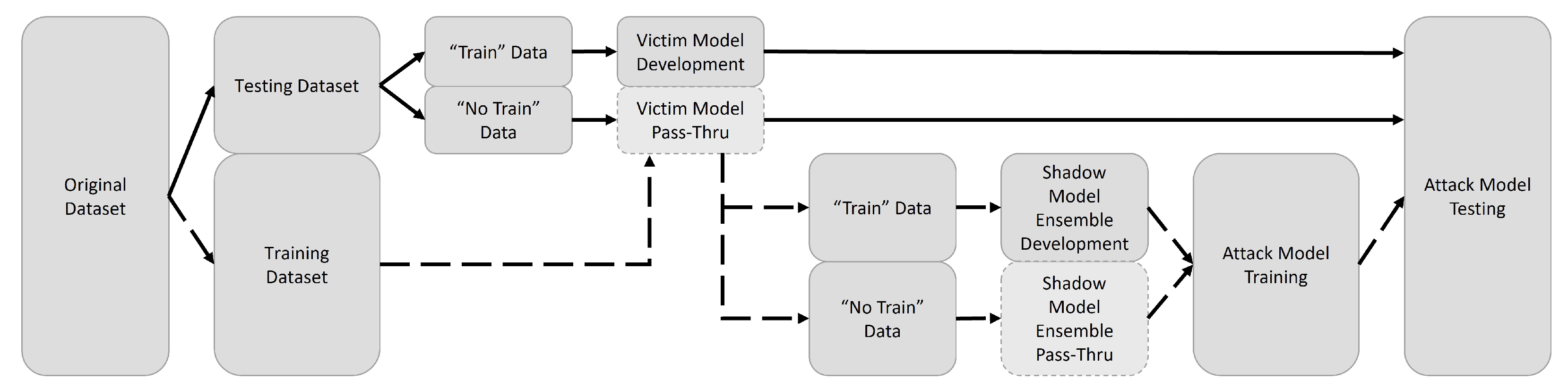
2.2. Membership Inference Attack

Membership inference attacks can be characterized based on adversarial knowledge of the model being attacked. This knowledge can be white-box, gray-box, or black box—listed in order of increasing difficulty. This study follows the same adversarial knowledge conventions as Truex et al. [20]. White-box knowledge indicates that the adversary has access to some portion or version of the real training data, gray-box indicates that the adversary has some statistical information on the training data, and black-box indicates that the adversary has nothing more than publicly available information on the training data.

This study assumes white-box knowledge of the training data. By erring to an easier attack by the adversary, the vulnerability-classification model developed will be based on the most vulnerable type of dataset. Anything other than white-box knowledge will result in a more secure dataset. Note that these definitions refer to the adversary’s training data knowledge and not their access or understanding of developed victim models. This study assumes black-box access to victim models, meaning that an adversary has access only to the inputs and results vectors of those models. This assumption is justified through the common use of black-box deployment for models when those models are open to access outside the parent organization.

The membership inference attack utilized to develop the vulnerability metric follows the shadow model methodology as developed by Shokri et al. and was chosen due to its general acceptance as a valid membership inference attack methodology as well its ability to successfully attack black-box models [65]. This attack begins with the development of a shadow model training dataset, which was developed through the utilization of some knowledge of the original training dataset—white-box knowledge of the training data—providing an easier situation for the attacker and, thus, a more reliable vulnerability metric.

In this effort, the shadow model training data was developed from a random extraction of 60% to $80\%$ from the original training dataset, dependent on the original size of the dataset. This left 20% to $40\%$ of the original data to be used as test data. For this study, one half of the test data was used to train the victim model and labeled as Trained. The other half of the test data was simply processed through the already trained model and labeled as Not-Trained. In this way, a test dataset of observations labeled as Trained/Not-Trained were developed to evaluate the performance of the attack model. Figure 1 provides a visual description of the data split.

Continuing with Figure 1, the training dataset was then passed through the victim model in order to obtain proper classification. No knowledge of the victim model was required—instead, simply access for input and receipt of output probability vectors (a black-box model) were needed. Next, one-half of this, now properly labeled, shadow model training dataset was utilized to train an ensemble of shadow models that seeks to mimic the characteristics of the victim model. Through the utilization of an ensemble of shadow models made up of various model types and hyperparameter settings, the ensemble can account for different possibilities of victim model architectures and behaviors. This shadow model ensemble development is discussed in greater detail below.

Once the shadow models were developed, the one-half of the training dataset that was utilized to train the shadow models, was labeled as Trained, and the half that was not used was labeled as Not-Trained. The entire shadow model training dataset was then passed through the shadow model ensemble in order to obtain an output probability vector. This vector along with the label of Trained/Not-Trained and the original set of dataset features were utilized as an attack model dataset in order to create a binary classification model that can determine whether an observation was utilized in training of the victim model as shown in Figure 2.

2.2.1. Development and Standardization of Victim Models

To maintain the concentration of the study on the vulnerability of the datasets themselves as opposed to the models, all victim models utilized in Table 1 were developed and standardized in the same way. The datasets utilized consisted of solely numerical and/or binary features, or if they contained categorical features, the categorical features were one-hot encoded. Prior to classification algorithm training, the datasets were standardized utilizing the default settings of the MinMaxScaler function of scikit-learn.

The following four classification algorithms were used, all from scikit-learn, and all utilizing their default settings with exceptions as noted in parenthesis: RandomForest (100 estimators and no preset depth), LogisticRegression (L2 penalty and lbfgs solver), SVC (rbf kernel and gamma scale), and NaiveBayesGB ($\alpha =1.0$ and “True” priors). In addition, a neural network classifier was utilized, which was again kept standard to include a single hidden layer with 128 nodes activated by a ReLu activation and a learning rate of 0.005. Given that all datasets were divided into individual classes within this study, all output layers were binary and were thus activated using a Sigmoid activation. Adam optimization was utilized with a binary crossentropy loss function and a 0.005 learning rate. The neural net classifier was implemented using the TensorFlow Python package.

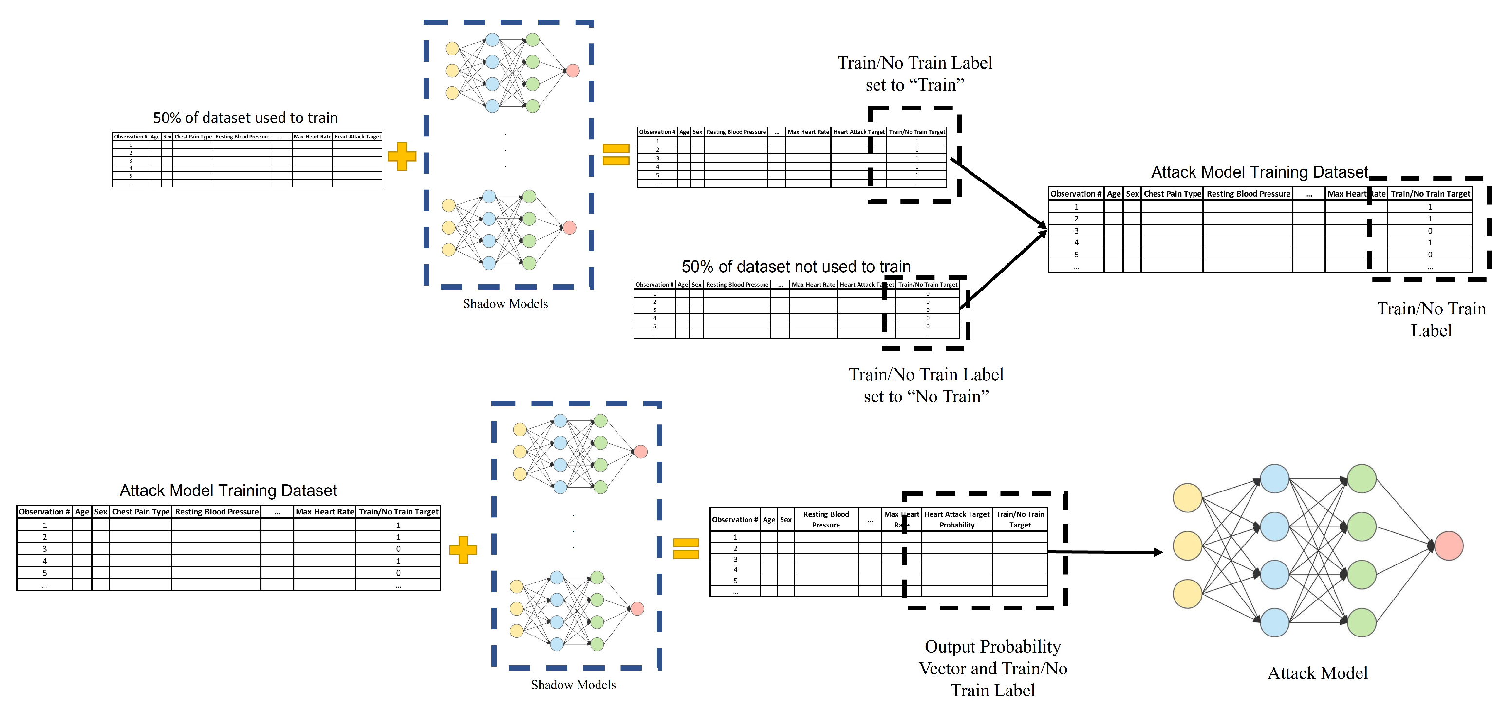
2.2.2. Development and Standardization of Shadow Models

In their seminal work using the shadow model membership inference attack, Shokri utilized neural networks for both the shadow model ensemble and the attack model [65]. In her work building on Shokri’s efforts, Truex found that the shadow model type and attack model type had little effect on the success of the attack but showed promising results through the use of decision trees [20]. However, in order to remove the effect of shadow and attack model type selection from the vulnerability metric, this study utilized combinations of shadow and attack models as described in Table 1. In addition, each shadow model has several hyperparameters, which were chosen at random—visualized in

Table 2. Hyperparameter variation within the shadow model ensemble.

Model Type	Hyperparameter	Potential Values
Random Forest	Number of Estimators	100, 500, 1000
	Depth	10, 50, 100, None
Neural Net	Number of Hidden Layers	1
	Number of Nodes in Layer	64, 128, 256
Logistic Regression	Penalty	L1, L2
	Solver	newton-cg, sag, lbfgs, saga
SVM	Kernel	rbf, poly, sigmoid
	Gamma	scale, auto
Naive Bayes	Alpha	1, 0
	Priors	True, False

—in order to develop an ensemble of models that can mimic the victim model.

As mentioned previously and depicted in Figure 1 and Figure 2, a portion (60–$80\%$) of the original dataset was set aside for attack model development. Of this, $50\%$ was used to train the shadow model ensemble and was subsequently labeled as Trained data to indicate that it was used to train the ensemble. The ensemble consisted of 20 models, each with an evenly weighted vote, and with a random selection of hyperparameters as described in Table 2.

The type of model used in the ensemble was determined based on the given combination as shown in Table 1. Using many different models with various, randomly selected hyperparameters in the ensemble provides for better capture of the intricacies of the victim model, thereby, allowing for a better understanding of how that model may be incorporating the training data within its structure. For each dataset, 13 different combinations of victim, shadow, and attack models were created and evaluated to provide emphasis on the dataset instead of the model combination.

2.2.3. Development and Standardization of the Attack Model

Figure 1 and Figure 2 provide a visual description of the development of the attack model. Following the development of the shadow model ensemble, the $50\%$ of data that was used to train the ensemble and labeled as Trained was recombined with the $50\%$ of the data that was withheld from the ensemble training and labeled Not-Trained. This new dataset was then passed through the shadow model ensemble in order to obtain the output probability vector. This new dataset consisting of the original dataset features, the Trained/Not-Trained label, and the output probability vector was subsequently utilized to train the attack model with the Trained/Not-Trained label as the target variable and the remaining features as the input. The specific model type was determined based on the combination being evaluated as shown in Table 1.

To maintain experimental control over the attack to provide a more universal vulnerability metric, the attack models were kept standard across all datasets as was done for the victim model development. The neural net model utilized a single hidden layer of 64 nodes and a binary output node. The hidden layer was activated using a ReLu activation and the output layer by a sigmoid activation. The model was optimized using an Adam optimizer, a binary cross-entropy loss function, and a learning rate of 0.0001.

The random forest model utilized 100 estimators, no predefined depth, and the remainder of the parameters set to the default settings from scikit-learn. The logistic regression model made use of an L2-penalty, an lbfgs solver, and the remainder of the parameters set to the default settings from scikit-learn. The support vector classifier model utilized an rbf kernel, a gamma scale, and the remainder of the parameters set to the default settings from scikit-learn. Finally, the Naive Bayes model was created using an $\alpha =1.0$, “True” priors, and the remainder of the parameters set to the default settings from scikit-learn.

While the other attack models could be directly trained on the attack model dataset, the use of the neural net model required a set of two models—one for each binary outcome for the class-based sub-dataset. The neural net models are more capable of capturing the subtleties of the Trained/Not-Trained observations when focused on a particular class and, therefore, require a hard-coded class selection protocol in order to assign the observation to the correct attack neural net based on the predicted class [65]. Given that this study divided the individual classes of each dataset into individual sub-datasets for disparate attack evaluation, the classes of a given subset consisted of the positive and negative Boolean evaluation of membership within the given class.

2.3. Understanding of Labeling

To develop the vulnerability-classification model, the data needed to be labeled.

Table 3. Descriptive statistics of the attack accuracies found within the training set of the current disparate attack study.

Statistic	Disparate Attack
Mean	0.617
Standard Deviation	0.111
Minimum	0.324
$25\%$ Quartile	0.530
$50\%$ Quartile	0.582
$75\%$ Quartile	0.697
Maximum	0.915

provides a statistical description of the average accuracy of attack found within the training dataset of this study—averaged across the various combinations of attacks as defined in Table 1. As the attack model was developed on an even class split of data—considering the Trained/Not-Trained label division—and with a binary target, accuracy was deemed to be the most relevant metric on which to develop the vulnerability label.

Additionally, given the relatively narrow interquartile range of accuracy—stretching from 0.530 to 0.697—as shown in Table 3, we decided that a binary vulnerable/secure label would best suit the study with the threshold of vulnerability set to the mean of the average attack accuracy. Using an attack accuracy of $62\%$, we established the guessing percentage as $53\%$. The labels and training were all confined to the training set in order to maintain complete neutrality of the test set. The test set labels were based on the same threshold as found in the training set in order to maintain consistency.

2.4. Development of Dataset Features

This study evaluated the vulnerability of datasets to disparate membership inference attacks, requiring a dataframe consisting of observations made of class-based sub-datasets and features describing those subsets. Therefore, 118 features were developed to describe each dataset and class-based sub-dataset within the study. The features developed were meant to capture as many statistical subtleties of the datasets as possible to explore what properties of a dataset could lead to disparate membership inference attack vulnerability. In addition to features developed by the team, inspiration for features were also derived from work by Brazdil et al. [66].

Among others, the features developed and integrated include measures of depth, width, entropy, correlation, skewness, kurtosis, mutual information, principal component explanation, number of classes, observation distances, and proportions of categorical, binary, and numerical features. Full descriptions of the developed and utilized features can be found in

Table A1. Dataset feature definitions. Features that were applied to both the macro and class-based subsets are defined with “(Macro and Disparate)”. Those without this designation were applied only to the macro dataset.

Feature	Description
Number of Observations (Macro and Disparate)	The quantity of observations within the original dataset.
Class Entropy	Entropy as defined through the number of observations in each class.
Number of Classes	The number of classes.
Number of Features	The number of features in the original dataset.
Number of Features After One Hot Encoding	The number of features after the dataset has been processed using one-hot encoding on categorical features.
Proportion of Categorical Features	The proportion of categorical features in respect to the original number of features.
Proportion of Binary Features	The proportion of binary features in respect to the original number of features.
Proportion of Numerical Features	The proportion of numerical features in respect to the original number of features.
Variance of the Entropy of Features (Macro and Disparate)	An entropy is calculated for each feature. This is the variance of that array.
Maximum of the Entropy of Features (Macro and Disparate)	An entropy is calculated for each feature. This is the maximum value of that array.
Minimum of the Entropy of Features (Macro and Disparate)	An entropy is calculated for each feature. This is the minimum value of that array.
Mean of the Entropy of Features (Macro and Disparate)	An entropy is calculated for each feature. This is the mean of that array.
Maximum of the Numerical Feature Range (Macro and Disparate)	The maximum range of values of the numerical features.
Minimum of the Numerical Feature Range (Macro and Disparate)	The minimum range of values of the numerical features.
Global Maximum of the Numerical Feature Range (Macro and Disparate)	The global maximum range of values of the numerical features as defined by the largest numerical value minus the smallest numerical value across all numerical features.
Global Minimum of the Numerical Feature Range (Macro and Disparate)	The global minimum range of values of the numerical features as defined by the smallest, upper numerical value minus the largest, lower numerical value across all numerical feature ranges.
Mean of Mean Label Distances	The distances of observations within each label were calculated using cityblock distances and then averaged within that label. This feature is the mean of those averages.
Variance of Mean Label Distances	The distances of observations within each label were calculated using cityblock distances and then averaged within that label. This feature is the variance of those averages.
Mean of Mean Label Minimum Distances	The distances of observations within each label were calculated using cityblock distances. This feature is the mean of the minimum of distances for each label.
Variance of Mean Label Minimum Distances	The distances of observations within each label were calculated using cityblock distances. This feature is the variance of the minimum of distances for each label.
Mean of Mean Label Maximum Distances	The distances of observations within each label were calculated using cityblock distances. This feature is the mean of the maximum of distances for each label.
Variance of Mean Label Maximum Distances	The distances of observations within each label were calculated using cityblock distances. This feature is the variance of the maximum of distances for each label.
Mean of Feature–Feature Correlation (Macro and Disparate)	This feature is the mean of feature to feature correlation values.
Maximum of Feature–Feature Correlation (Macro and Disparate)	This feature is the maximum value of feature to feature correlation values.
Minimum of Feature–Feature Correlation (Macro and Disparate)	This feature is the minimum value of feature to feature correlation values.
Mean of Variance of Feature–Feature Correlation (Macro and Disparate)	This feature is the mean of the variance of feature to feature correlation values.
Variance of the Mean of Feature–Feature Correlation (Macro and Disparate)	This feature is the variance of the means of feature to feature correlation values.
Number of PCAs Required to Explain $75\%$ Variance	The number of principal components required to explain $75\%$ of the variance of the dataset.
Cond num 2norm (Macro and Disparate)	Condition number of 2-norm.
Width Ratio (Macro and Disparate)	The ratio of the number of observations of the original dataset to the number of features of the original dataset.
Width Ratio of One Hot Encoding (Macro and Disparate)	The number of observations of the original dataset to the number of features after one-hot encoding the categorical variables.
Maximum Number of Categories (Macro and Disparate)	The maximum number of categories that any categorical feature in the original dataset contained.
Minimum Number of Categories (Macro and Disparate)	The minimum number of categories that any categorical feature in the original dataset contained.
Mean Number of Categories (Macro and Disparate)	The average number of categories for each categorical feature in the original dataset.
Variance of Number of Categories (Macro and Disparate)	The variance of the number of categories for each categorical feature in the original dataset.
Mean Feature–Feature Correlation Grouped by Label	The mean of the feature to feature correlation when grouped by label.
Maximum Feature–Feature Correlation Grouped by Label	The maximum of the feature to feature correlation when grouped by label.
Minimum Feature–Feature Correlation Grouped by Label	The minimum of the feature to feature correlation when grouped by label.
Mean of the Variance of Feature–Feature Correlation Grouped by Label	The average of the variance of feature to feature correlations when grouped by label.
Variance of the Means of Feature–Feature Correlation Grouped by Label	The variance of the means of the feature to feature correlations when grouped by label.
Canonical Correlation (Macro and Disparate)	Canonical correlation.
Maximum Feature Skewness (Macro and Disparate)	The maximum skewness of the features in the dataset.
Minimum Feature Skewness (Macro and Disparate)	The minimum skewness of the features in the dataset.
Mean Feature Skewness (Macro and Disparate)	The mean skewness of the features in the dataset.
Variance Feature Skewness (Macro and Disparate)	The variance skewness of the features in the dataset.
Maximum Feature Kurtosis (Macro and Disparate)	The maximum kurtosis of the features in the dataset.
Minimum Feature Kurtosis (Macro and Disparate)	The minimum kurtosis of the features in the dataset.
Mean Feature Kurtosis (Macro and Disparate)	The mean kurtosis of the features in the dataset.
Variance Feature Kurtosis (Macro and Disparate)	The variance kurtosis of the features in the dataset.
Standard Deviation Ratio of Features (Macro and Disparate)	The geometric mean ratio of standard deviations of the individual populations to the pooled standard deviation.
Maximum Standard Deviation Ratio of Features by Label	The maximum of the standard deviation ratios of features as described above but grouped by label.
Minimum Standard Deviation Ratio of Features by Label	The minimum of the standard deviation ratios of features as described above but grouped by label.
Mean of the Standard Deviation Ratio of Features by Label	The mean of the standard deviation ratios of features as described above but grouped by label.
Variance of the Standard Deviation Ratio of Features by Label	The variance of the standard deviation ratios of features as described above but grouped by label.
Mean Mutual Information of Features (Macro and Disparate)	The mean mutual information of features.
Maximum Mutual Information of Features (Macro and Disparate)	The maximum mutual information of features.
Minimum Mutual Information of Features (Macro and Disparate)	The minimum mutual information of features.
Variance of the Mutual Information of Features (Macro and Disparate)	The variance of the mutual information of features.
Mean Mutual Information of Features Grouped by Label	The mean mutual information of features grouped by label.
Maximum Mutual Information of Features Grouped by Label	The maximum mutual information of features grouped by label.
Minimum Mutual Information of Features Grouped by Label	The minimum mutual information of features grouped by label.
Variance of the Mutual Information of Features Grouped by Label	The variance of the mutual information of features grouped by label.
Equivalent Number of Attributes	Entropy of class divided by the mean mutual information of class and attributes.

located in Appendix A. These features were applied to the overall dataset and subsets of the macro dataset created for each class within the dataset as indicated by the feature description. For example, if a particular dataset had ten classes, then this study divided that dataset into ten separate datasets consisting of a binary label for the class being evaluated and then applied the features to that dataset.

Several features within the training dataset contained disperse distributions, which allowed for sub-samples of the dataset to fail Kolmogorov–Smirnov tests. However, given that the nature of the vulnerability metric requires such a diverse population of datasets, a methodology for standardizing these observations for modeling was required. We discovered that this dispersion of distributions was caused through several datasets having large outliers. The removal of these outliers could cause misleading results as these outliers and features could provide insight into potential vulnerabilities.

Therefore, to avoid the saturating effect of these features, the data was scaled using scikit-learn’s MinMaxScaler with its default settings. The scaling factor was generated using the training dataset and then applied to both the training set prior to model development and to the holdout test set prior to testing.

2.5. Feature Selection

As indicated below in Methodology: Vulnerability Classification, the resulting number of observations within the training dataset was 767. In order to avoid a wide dataset and potential overfitting or difficulty in classification, the feature set was reduced. Feature selection was performed utilizing an ensemble methodology of Pearson Correlation, ${\chi }^2$, and recursive feature selection was performed using logistic regression. Pearson Correlation selection was implemented using Numpy’s corrcoef function between the features and labels with default settings for each feature.

${\chi }^2$ selection was implemented by first scaling the data using scikit-learn’s MinMaxScaler with default settings. Then, scikit-learn’s SelectKBest function with the ${\chi }^2$ score function and other parameters set to default was fit to the data. Selections were returned using the SelectKBest’s $ge{t}_{s}upport$ function. Recursive feature selection was implemented using scikit-learn’s RFE, recursive feature elimination, function with a logistic regression estimator, number of features to select set to ten, and with the step set to ten. The Boolean result of keeping or removing the feature for each of these three methods was then placed in a dataframe in descending order based on the number of ”keep“ votes attributed to the feature.

This methodology was used to down-select the original 118 features to 15. These 15 features were then reduced to seven through an iterative modeling effort and are shown in

Table 4. The top seven features selected by the feature selection methodology, listed in order of importance based on the feature importance ranking of the feature selection ensemble.

Feature
Average of Label Minimum Distances
Variance of Label Minimum Distances
Variance of Label Mean Distances
Proportion of Binary Features
Average of Label Mean Distances
Average of Label Maximum Distances
Width Ratio After One Hot Encoding on Class Subsets

in order of importance based on feature importance ranking of the feature selection ensemble. This iterative modeling involved using the training data in various models with an array of hyperparameter settings in an effort to find the optimal mapping of observations and labels. This model then optimized the number of features by starting with the top 15 features and working down to the eventual seven features found as optimal as discussed in more detail below.

2.6. Vulnerability Classification

All methods up to this point were used to develop the vulnerability-classification dataset. This dataset consisting of observations of class-based sub-datasets, features detailing those subsets, and the labels associated with disparate membership inference attack accuracies averaged over various combinations of victim/shadow/attack models was then utilized to develop the vulnerability-classification model.

Several modeling methods were evaluated, including Random Forests, Logistic Regression, Decision Trees, Naive Bayes, and ensemble methodologies, to develop the vulnerability-classification model. These methods were evaluated with all top 15 features, as well as the top 10 and top five features. Ultimately, an ensemble model of a logistic regression model using a liblinear solver, a Naive Bayes model, and a random forest classifier using a minimum of five samples per leaf and 200 estimators was found to provide the best results.

Any hyperparameters not directly mentioned were set to the default scikit-learn settings. This model was then used to down-select the features to the seven shown in Table 4. The model was found utilizing leave-one-out cross validation (LOOCV) over the training dataset and resulted in the training and testing results as shown in

Table 5. Resulting metrics from the disparate vulnerability model development and testing for the ensemble model and seven features as shown in Table 4.

Metric	LOOCV Training Data	Test Data
Precision of Vulnerable Class	0.819	0.819
Recall of Vulnerable Class	0.762	0.759
F1 of Vulnerable Clas	0.789	0.788
Accuracy	0.846	0.845

.

Given the small size of the vulnerability metric training dataset, ADASYN (Adaptive Synthetic) data sampling was utilized to develop additional data observations [67]. The synthetic data were developed within each training fold through the use of the default settings of the ADASYN function in the imbalanced-learn library [68].

2.7. Hardening Exploration

Based on the results found in the vulnerability study and discussed in more detail below, four different methods of hardening against membership inference attack were chosen for exploration. These methods focused on the reduction of the width ratio, increase of feature entropy, and reduction of disparities in class size. Unlike in a macro-level vulnerability study, each dataset in this study consisted of only “one class” given that the datasets were actually class-based sub-datasets as described above. However, this “one class” was represented with a binary label of “represented by this class” or “not represented by this class”, and therefore class size disparity still existed and was still considered within the hardening process.

The first method was a feature reduction method, which removed features based on correlation. Features that were more than $80\%$ correlated with other features were removed. The second was a feature reduction method based on manifold theory. Using isometric mapping across a scale of increasing number of components up to a count equal to the original number of features, an elbow plot was created to determine the optimal number of components to maintain. This number of components was then used again in the isometric mapping process to reduce the feature size of the dataframe. Isometric mapping was applied using the default setting from the scikit-learn library for Python.

The third method was an oversampling method using a conditional tabular generative adversarial network (CTGAN) [69]. CTGAN was chosen for oversampling to provide an equal number of observations in classes through oversampling while maintaining the same data structure. Other methods, such as ADASYN and SMOTE, rely more on linear connections between observations, while CTGAN learns the original distribution of the subset of data to be sampled. The CTGAN method was implemented using the default settings with 100 epochs from the SDV library for Python.

The final approach was to use NearMiss version two undersampling implemented through the the imblearn library for Python, with version two selected and “not minority” as the sampling strategy. NearMiss version two was selected to provide an undersampling strategy that maintains the original data structure. Based on the efforts of the original developers of the NearMiss strategy, version two provided the best results for the requirements of this study [70].

3. Results of Vulnerability Classification

Shown below are the results of the vulnerability classification process, presented through an understanding of the features utilized in the classification model. Interestingly, macro-level dataset features were found to show higher importance in the determination of individual class vulnerability than those developed and processed solely on the class-based sub-datasets. Therefore, within the tables of descriptive statistics based on these macro dataset features shown below, some values are found to be the same across vulnerable and non-vulnerable splits because, within a given dataset, some classes may be vulnerable and others safe. This section presents the results as found within the study. Further discussion of these findings is provided in the Discussion section.

3.1. In-Label Distance Measures

In-label distance measures compute the distances between each observation within a class. This metric follows from insight found in work, such as that by Truex and Yaghini discussed above [20,21]. These measures first group observations by class and then determine the distances between each observation within the class using a city block, also known as a Manhattan, distance measurement as shown in Equation (3). This distance metric was utilized in agreement with Aggarwal et al. who found that this L1 norm metric provides better results in high dimensional datasets [71].

$$d=\sum _{i=1}^n|x_i-y_i$$

(3)

As discussed in the Introduction and reiterated above, it is understood that sparse class boundaries can lead to vulnerabilities within a class, and this is a driving factor for disparate vulnerability. Therefore, it is reasonable that five of the seven top features are related to in-label distance measures for the disparate attack vulnerability-classification model.

Table 6. Descriptive statistics of the in-label distance measure features for the overall dataset, the non-vulnerable observations, and the vulnerable observations.

Feature	Descriptive Statistic	Full Dataset	Non-Vulnerable	Vulnerable
Average of Label Minimum Distances	Mean	19.85	0.62	48.80
	Standard Deviation	41.13	5.41	52.95
	Minimum	0.00	0.00	0.00
	$\mathbf{25}\%$ Quartile	0.00	0.00	0.00
	$\mathbf{50}\%$ Quartile	0.00	0.00	4.15
	$\mathbf{75}\%$ Quartile	2.00	0.07	111.35
	Maximum	111.35	103.22	111.35
Variance of Label Minimum Distances	Mean	260.81	5.76	644.85
	Standard Deviation	552.29	91.81	711.89
	Minimum	0.00	0.00	0.00
	$\mathbf{25}\%$ Quartile	0.00	0.00	0.00
	$\mathbf{50}\%$ Quartile	0.00	0.00	0.19
	$\mathbf{75}\%$ Quartile	0.01	0.00	1409.65
	Maximum	1536.01	1536.01	1536.01
Variance of Label Mean Distances	Mean	293.26	9.08	721.16
	Standard Deviation	621.88	121.66	801.77
	Minimum	0.00	0.00	0.00
	$\mathbf{25}\%$ Quartile	0.47	0.22	1.11
	$\mathbf{50}\%$ Quartile	1.11	1.11	8.16
	$\mathbf{75}\%$ Quartile	8.16	1.11	1521.40
	Maximum	2282.77	2282.77	2282.77
Average of Label Mean Distances	Mean	41.39	8.04	91.60
	Standard Deviation	70.95	12.02	90.60
	Minimum	0.26	0.26	0.65
	$\mathbf{25}\%$ Quartile	7.15	4.20	8.73
	$\mathbf{50}\%$ Quartile	8.73	8.73	10.81
	$\mathbf{75}\%$ Quartile	10.92	8.73	191.09
	Maximum	191.51	191.51	191.51
Average of Label Maximum Distances	Mean	65.17	17.45	137.01
	Standard Deviation	101.79	19.58	129.68
	Minimum	2.14	2.14	2.31
	$\mathbf{25}\%$ Quartile	13.13	11.50	18.92
	$\mathbf{50}\%$ Quartile	18.92	18.92	23.77
	$\mathbf{75}\%$ Quartile	23.77	18.92	273.40
	Maximum	325.20	325.20	325.20

provides a summary of the descriptive statistics for each of the included in-label distance features. It can be seen that, for the average of the label minimum, mean, and maximum distances, the distance is significantly higher for vulnerable datasets when compared to their non-vulnerable counterparts. Furthermore, included as significant features are the variance of the label minimum and mean distances, which were also significantly higher for vulnerable datasets. The variance of label distance features and the average of label minimum distances show the most divergence in the upper $50\%$ of the data.

3.2. Width Ratio

The width ratio of a dataset can provide insight into an overabundance of information. The hypothesis being that the provision of many features in description of a limited set of observations can facilitate an adversary’s inference of training data membership through this overabundance of information. In this study, the width ratio was implemented as a ratio of the number of features to the number of observations, meaning that a higher width ratio indicates a wider dataset. The feature found to be the most prominent in this family of width ratios was calculated after one-hot encoding of categorical variables and completed on class-based data subsets.

Table 7. Descriptive statistics of the width ratio after one-hot encoding on the class-based data subset feature for the overall dataset, the non-vulnerable observations, and the vulnerable observations.

Descriptive Statistic	Full Dataset	Non-Vulnerable	Vulnerable
Mean	0.21	0.13	0.34
Standard Deviation	0.49	0.32	0.65
Minimum	0.00	0.00	0.01
$25\%$ Quartile	0.01	0.01	0.06
$50\%$ Quartile	0.05	0.02	0.24
$75\%$ Quartile	0.28	0.10	0.31
Maximum	5.36	4.32	5.36

shows that vulnerable datasets have significantly wider datasets than their non-vulnerable counterparts—in agreement with the stated hypothesis.

3.3. Proportion of Binary Features

The proportion of binary features was included in the dataset feature set to understand how different types of features and different ratios of feature types can affect dataset vulnerability to membership inference attacks. Understanding how these types and ratios of feature types relate to vulnerability can assist data owners in the development and setup of their datasets dependent on security vs. utility needs. The proportion of binary features provides the ratio of the number of binary features to the total number of features.

Table 8. Descriptive statistics of the proportion of binary features feature for the overall dataset, the non-vulnerable observations, and the vulnerable observations.

Descriptive Statistic	Full Dataset	Non-Vulnerable	Vulnerable
Mean	0.21	0.03	0.47
Standard Deviation	0.39	0.13	0.49
Minimum	0.00	0.00	0.00
$25\%$ Quartile	0.00	0.00	0.00
$50\%$ Quartile	0.00	0.00	0.13
$75\%$ Quartile	0.13	0.00	1.00
Maximum	1.00	1.00	1.00

shows that vulnerable datasets have, on average, a higher number of binary features. In addition, the largest diversion occurs in the upper $50\%$ of the data.

4. Results of Hardening Exploration

Following the discoveries from the vulnerability study above, exploratory efforts to harden the datasets based on these findings while maintaining utility were attempted. This exploration allowed for both a first approach to dataset hardening methodologies against disparate attacks and a deeper understanding of what methods work for different types of datasets. As mentioned in the Results of Vulnerability Classification section, this section provides the results as found in the study. Further explanation of these results is provided in the Discussion section.

Table 9. The results of hardening efforts showing the number of class-based subsets (along with the original number of datasets prior to class-based breakdown) and the results of each hardening method explored. These results include the number of subsets that remained the same, those that became more secure, and those that became more vulnerable, along with the changes in the victim model accuracy, F1 score, and attack accuracy on average.

Hardening Method	Class-Based Subsets Hardened (Original Datasets) $[\#]$	Subsets Unchanged $[\%]$	Subsets Which Became More Secure $[\%]$	Subsets Which Became More Vulnerable $[\%]$	Change in Victim Model Accuracy on Average	Change in Victim Model F1 Score on Average	Change in Disparate Attack Accuracy on Average
Feature Reduction via Correlation	439 (97)	85.9	7.5	6.6	Insignificant	Insignificant	−0.01
Feature Reduction via Manifold Theory	355 (77)	82.5	16.1	1.4	−0.03	−0.04	−0.04
Class Balancing via Oversampling	436 (96)	86.9	7.6	5.5	+0.02	+0.02	+0.01
Class Balancing via Undersampling	621 (102)	87.1	4.8	8.1	+0.02	+0.02	+0.02
Correlation-Based Feature Reduction with Oversampling	239 (63)	81.6	13.0	5.4	Insignificant	−0.01	−0.01
Manifold Theory-Based Feature Reduction with Oversampling	208 (57)	79.8	19.2	1.0	−0.01	Insignificant	−0.02

provides information on the number of datasets hardened; the number of class-based subsets within these datasets; the percent of subsets that were unchanged, made more secure, and made more vulnerable; and information on the changes in the victim model and attack accuracies. From this table, it can be seen that the two combinational hardening methods and the feature reduction via manifold theory performed the best in reducing the vulnerability to disparate membership inference attacks. Of these three, the two combinational hardening methods provided better maintenance of the original (victim) model utility, as evinced through the low/insignificant changes in the victim model accuracy and F1 score on average.

5. Discussion of Vulnerabilities to Disparate Membership Inference Attack

This section discusses the findings associated with the vulnerability classification of datasets to disparate membership inference attacks. As shown in Table 5, the developed vulnerability-classification model can determine the vulnerability of a dataset to disparate membership inference attacks with an accuracy of $84.5\%$. This model provides data owners with the ability to evaluate their datasets’ vulnerability to privacy leakage via this attack. Many datasets, including those with PII and PHI, such as medical datasets, and those that contain proprietary or confidential information, such as commercial and military datasets, can lead to individual, organizational, or national detrimental effects if their information is leaked. Therefore, having an understanding of this vulnerability to potential record discovery is of great importance to these data owners.

In addition to the vulnerability classification contribution, the features that make up this model equally contribute in their provision of understanding of this vulnerability. This section discusses these features and their importance to the understanding of this vulnerability.

Five of the seven features selected through the vulnerability-classification modeling effort were based on in-label observational distance measurements. This finding is in agreement with previous understandings that minority and sparsely populated classes tend to have higher vulnerability within a given dataset. Two main ideas are shown in the evaluation of the in-label distance features. The first is that the average label minimum, mean, and maximum distances are all greater for vulnerable datasets than for non-vulnerable datasets. This shows that sparse class regions are more prone to attack than their denser counterparts.

The second is that the variance of the minimum and mean distances—and for the non-included variance of the maximum distance feature—is greater for vulnerable datasets. These variances show the most diversity in the upper $50\%$ of the data. Therefore, it can be concluded that, in addition to the fact that more sparse class regions lead to more vulnerable data subsets, a lack of even distribution of observations within the class region can also lead to disparate vulnerability.

This is an important observation and contribution to the current understanding of vulnerability to both macro-level and disparate membership inference attacks. The current literature indicates the contribution of sparse class regions to attack vulnerability [19,20,21]. However, this finding demonstrates that not only can a lack of supporting members lead to the vulnerability of those subclasses but also a lack of uniformity in the density of observations within a particular class boundary region can lead to vulnerability.

The width ratio of class-based sub-datasets after one-hot encoding was also found to be an important feature in classifying disparate vulnerability. A wider dataset can result in an over explanation of observations by providing more information than is necessary for the feature-to-label mapping. This overabundance of information creates opportunities for membership inference attack. The fact that this was a feature developed on the class sub-sets as opposed to the macro dataset—resulting in wider datasets for those less populated class-based subsets—agrees with previous understandings that under-represented portions of a dataset, such as less populated classes, are more vulnerable to attack.

Finally, the proportion of binary features was found to be an important factor in determining disparate vulnerability. While this feature was developed on the macro dataset, dividing the dataset into class-based subsets would not change its value, given that it is the proportion of binary features to the total number of features. When exploring the reasoning of importance behind the inclusion of this feature, it is interesting to consider the width ratio after one-hot encoding as discussed above. Binary features are, by nature, “on” or “off”.

One-hot encoding of categorical features creates a set of binary features indicating “on” or “off” for each element within the encoded categorical variable. Therefore, one-hot encoding of categorical variables will increase the proportion of binary features within the dataset, while the method for calculating the proportion of binary features was coded to not include the categorically one-hot encoded features. The idea that both of these “on/off” features are included as important for determining vulnerability leads to an understanding of how these discrete attributes can lead to vulnerability.

When considering that, within the literature on algorithmic and model vulnerability as discussed in the Introduction: Previous Work, entropy and correlation themes were seen as the most important, it can be speculated that features that include more entropy within the observational attribute itself could be more secure. In other words, features that are binary and one-hot encoded categorical features provide only two states in comparison to the infinite number of states one may find when a feature can take on a continuous value, such as between 0 and 1.

This, as described above for the uniformity of class regions, is an important contribution to the current understanding of the vulnerability of datasets to not only disparate membership inference attack but also membership inference attack in general—namely, that datasets with a larger proportion of continuous variables as opposed to discrete variables are more secure against membership inference attack due to the increase in entropy within those features.

6. Discussion of Hardening Exploration

This section discusses the results associated with the hardening exploration efforts. While the impetus of the article focuses on the understanding of dataset vulnerability to disparate membership inference attack, an exploration into hardening techniques based on these discovered vulnerabilities can assist in this understanding while also offering an introduction to mitigation strategies for the dataset owner.

These hardening explorations were developed based on the features found to contribute to vulnerability, which can be summarized into an over-abundance of information relating to the width-ratio feature, sparse and unevenly distributed class regions relating to the in-label distance features, and a lack of entropy within individual feature realization possibilities as found in the proportion of binary features and one-hot encoded categorical variables. This study focused on the former two vulnerabilities through feature reduction efforts based on correlation and manifold theory and through class-balance methods based on oversampling via CTGAN and undersampling using NearMiss methodologies. In addition, combinations of feature reduction and oversampling methods were also explored given their more promising results to evaluate if further hardening could be accomplished.

Feature reduction based in manifold theory provided better results than using correlation thresholds. Given that manifold theory finds a lower dimensional representation of the information contained within the feature set, this reduction to a more base layer could provide a perturbation effect on the membership inference attack attempt. In addition, by condensing the feature set, this hardening method could have changed the uniformity of in-region observational distribution to be more uniform and thus provided protection in this manner.

However, end-users may find hardening via manifold theory to be less appealing due to the increased difficulty in understanding and explanation of the results of the classification exercise given the decreased definition of what is contained within a particular feature of importance within their ultimate algorithm.

Oversampling provided for a larger increase in the percent of secured datasets and a lower percent in the number of datasets, which increased in vulnerability as compared to undersampling, while both methods attempted to balance classes, oversampling increased the fortification of existing observations. Therefore, it is reasonable that this increase in supporting members—and thus entropy—would reduce the ability of an attack to discern if an observation was or was not a part of the original training dataset. However, the oversampling method did not provide the level of improvement seen in the manifold theory-based feature reduction method. Given that the oversampling technique utilized maintained the original distributions, there would still be a similar non-uniformity of the in-class region distribution of observations, therefore, leaving this vulnerability-contributing factor unresolved.

However, the best results were found with a combination of the two best-performing methods of feature reduction and class balancing efforts—a manifold theory-based feature reduction with CTGAN oversampling. This provided an effectively insignificant change in the victim model performance while reducing the disparate attack accuracy by 0.02 on average. A total of $19\%$ of class subsets were made more secure, and only $1\%$ were more vulnerable. This elevated protection can be attributed to the perturbing effect and increase of uniformity of the in-class region observational distribution of the manifold-theory-based feature reduction as well as the increase of supporting observations and entropy of the oversampling method.

7. Summary and Future Efforts

This study provides an in-depth look at the vulnerability of datasets themselves to disparate membership inference attacks—those that focus on attacking individual classes as opposed to the overall dataset—contributing an addition to the current literature that focuses on model vulnerability. This understanding was accomplished through the creation of a vulnerability-classification model based on over 100 datasets—including frequently cited datasets within the AI security literature. The vulnerability-classification dataset used to create this classification model consisted of 118 features and a set of victim, shadow, and attack model accuracies, all used to describe and understand the vulnerability of these datasets to disparate membership inference attacks.

The resulting ensemble model, consisting of a logistic regression model, Naive Bayes model, and a random forest model, obtained a testing accuracy of $84.5\%$ in classifying datasets as vulnerable or secure to these disparate membership inference attacks. Of the seven features used in the classification model, five were based on in-label observational distance measurements. This heavy reliance on observational distances within class regions is consistent with other findings in the literature, which state that minority and sparsely populated classes tend to increase vulnerability.

In addition to the vulnerability-classification model, this study also provided an increased understanding of the vulnerability of datasets to these attacks. First, it was shown that the uniformity of the in-class region distribution is an important factor in dataset vulnerability. Those datasets with a less uniform distribution of in-class observational distances were proven to be more vulnerable to attack. Second, it was shown that an increased proportion of binary features can result in an increase in vulnerability.

This finding was established through the width ratio after one-hot encoding and the proportion of binary features exclusive of categorical one-hot encoded features (both of which indicated an increase in vulnerability with the increase of either the width of the dataset after one-hot encoding) or the increase in the proportion of binary features, while wider datasets in general can contribute to an overabundance of information and, therefore, an adversarial advantage for membership inference. Of particular interest was the inclusion of the post-one-hot encoding aspect. One-hot encoding results in a binary feature indicating a categorical response and is a common preprocessing step for datasets.

Given understandings of entropic contributions to membership inference vulnerability and previous findings of low entropy features causing an increase in vulnerability, we concluded that these binary features, due to their low inherent entropy, result in an increase in attack success. Non-binary features can take on an infinite number of values and, thus, provide more entropy-influenced security compared with two-state binary features.

To further understand these vulnerabilities and to provide exploratory mitigation strategies, we investigated preliminary hardening strategies based on the vulnerabilities discovered in the vulnerability classification process. In particular, feature reduction methods were used to treat an overabundance of information and intelligent over- and undersampling methods were used to treat class-region sparsity and imbalances. The best-performing method proved to be a manifold theory-based feature reduction combined with a CTGAN-based oversampling strategy.

This hardening process resulted in a reduction in disparate attack accuracy of 0.02 on average and an effectively insignificant change in the victim model performance. Using this method, $19\%$ of class-based sub-datasets were made more secure, and only $1\%$ were more vulnerable.

We concluded that manifold theory-based feature reduction provided improved results over correlation-based feature reduction due to the perturbing effects resulting from the consolidation of the feature set into a lower dimension as well as the potential densification and increased uniformity of in-class observational distances due to the re-mapping of labels to this new, reduced feature set. CTGAN oversampling’s increased success over NearMiss version two undersampling was attributed to the increase in fortifying observations in contrast to a general reduction in majority class size, as well as through an increase in the entropy of affected features and classes through the increase of observations.

This work provides data owners with the ability to classify their datasets’ vulnerability to disparate membership inference attacks. In addition, this provides an understanding of this vulnerability and provides exploratory mitigation methods. Most notably, this is the first work to exclusively study dataset vulnerability to these attacks as opposed to model vulnerability. Through this effort, additional investigations, such as the in-class uniformity of observational distance and binary vs. continuous feature contributions to vulnerability were provided for a broader understanding of membership inference attacks. Future development efforts should be focused on understanding how hardening at the class level affects hardening at the macro level, as well as deeper investigations into other hardening methods, which may provide even better results.

References

1. Veale, M.; Binns, R.; Edwards, L. Algorithms that remember: Model inversion attacks and data protection law. Philos. Trans. R. Soc. A Math. Phys. Eng. Sci. 2018, 376, 20180083. [Google Scholar] [CrossRef] [PubMed] [Green Version]
2. Chakraborty, A.; Alam, M.; Dey, V.; Chattopadhyay, A.; Mukhopadhyay, D. Adversarial attacks and defences: A survey. arXiv 2018, arXiv:1810.00069. [Google Scholar] [CrossRef]
3. He, Y.; Meng, G.; Chen, K.; Hu, X.; He, J. Towards Privacy and Security of Deep Learning Systems: A Survey. arXiv 2019, arXiv:1911.12562. [Google Scholar]
4. Qiu, S.; Liu, Q.; Zhou, S.; Wu, C. Review of artificial intelligence adversarial attack and defense technologies. Appl. Sci. 2019, 9, 909. [Google Scholar] [CrossRef] [Green Version]
5. Calandrino, J.A.; Kilzer, A.; Narayanan, A.; Felten, E.W.; Shmatikov, V. “You might also like:” Privacy risks of collaborative filtering. In Proceedings of the 2011 IEEE Symposium on Security and Privacy, Washington, DC, USA, 22–25 May 2011; pp. 231–246. [Google Scholar]
6. Sweeney, L. k-anonymity: A model for protecting privacy. Int. J. Uncertain. Fuzziness Knowl.-Based Syst. 2002, 10, 557–570. [Google Scholar] [CrossRef] [Green Version]
7. Fredrikson, M.; Lantz, E.; Jha, S.; Lin, S.; Page, D.; Ristenpart, T. Privacy in pharmacogenetics: An end-to-end case study of personalized warfarin dosing. In Proceedings of the 23rd USENIX Security Symposium (USENIX Security 14), San Diego, CA, USA, 20–22 August 2014; pp. 17–32. [Google Scholar]
8. Narayanan, A.; Shmatikov, V. Robust De-anonymization of Large Datasets (How to Break Anonymity of the Netflix Prize Dataset). The University of Texas at Austin. In Proceedings of the 29th IEEE Symposium on Security and Privacy, Oakland, CA, USA, 18–21 May 2008; pp. 111–125. [Google Scholar]
9. Salem, A.; Zhang, Y.; Humbert, M.; Berrang, P.; Fritz, M.; Backes, M. Ml-leaks: Model and data independent membership inference attacks and defenses on machine learning models. arXiv 2018, arXiv:1806.01246. [Google Scholar]
10. Hilprecht, B.; Härterich, M.; Bernau, D. Monte carlo and reconstruction membership inference attacks against generative models. Proc. Priv. Enhancing Technol. 2019, 2019, 232–249. [Google Scholar] [CrossRef] [Green Version]
11. Fredrikson, M.; Jha, S.; Ristenpart, T. Model inversion attacks that exploit confidence information and basic countermeasures. In Proceedings of the 22nd ACM SIGSAC Conference on Computer and Communications Security, Denver, CO, USA, 12–16 October 2015; pp. 1322–1333. [Google Scholar]
12. Kuppa, A.; Le-Khac, N.A. Adversarial xai methods in cybersecurity. IEEE Trans. Inf. Forensics Secur. 2021, 16, 4924–4938. [Google Scholar] [CrossRef]
13. Huang, W.; Zhou, S.; Liao, Y. Unexpected Information Leakage of Differential Privacy Due to the Linear Property of Queries. IEEE Trans. Inf. Forensics Secur. 2021, 16, 3123–3137. [Google Scholar] [CrossRef]
14. Rezaei, S.; Liu, X. An Efficient Subpopulation-based Membership Inference Attack. arXiv 2022, arXiv:2203.02080. [Google Scholar]
15. Tan, J.; Mason, B.; Javadi, H.; Baraniuk, R.G. Parameters or Privacy: A Provable Tradeoff between Overparameterization and Membership Inference. arXiv 2022, arXiv:2202.01243. [Google Scholar]
16. Ateniese, G.; Mancini, L.V.; Spognardi, A.; Villani, A.; Vitali, D.; Felici, G. Hacking smart machines with smarter ones: How to extract meaningful data from machine learning classifiers. Int. J. Secur. Netw. 2015, 10, 137–150. [Google Scholar] [CrossRef]
17. Long, Y.; Bindschaedler, V.; Wang, L.; Bu, D.; Wang, X.; Tang, H.; Gunter, C.A.; Chen, K. Understanding membership inferences on well-generalized learning models. arXiv 2018, arXiv:1802.04889. [Google Scholar]
18. Long, Y.; Wang, L.; Bu, D.; Bindschaedler, V.; Wang, X.; Tang, H.; Gunter, C.A.; Chen, K. A Pragmatic Approach to Membership Inferences on Machine Learning Models. In Proceedings of the 2020 IEEE European Symposium on Security and Privacy (EuroS&P), Genoa, Italy, 7–11 September 2020; pp. 521–534. [Google Scholar]
19. Tonni, S.M.; Farokhi, F.; Vatsalan, D.; Kaafar, D. Data and Model Dependencies of Membership Inference Attack. arXiv 2020, arXiv:2002.06856. [Google Scholar]
20. Truex, S.; Liu, L.; Gursoy, M.E.; Yu, L.; Wei, W. Demystifying membership inference attacks in machine learning as a service. IEEE Trans. Serv. Comput. 2019, 14, 2073–2089. [Google Scholar] [CrossRef]
21. Yaghini, M.; Kulynych, B.; Troncoso, C. Disparate vulnerability: On the unfairness of privacy attacks against machine learning. arXiv 2019, arXiv:1906.00389. [Google Scholar]
22. Bagdasaryan, E.; Poursaeed, O.; Shmatikov, V. Differential privacy has disparate impact on model accuracy. In Proceedings of the Advances in Neural Information Processing Systems, Vancouver, BC, Canada, 8–14 December 2019; pp. 15479–15488. [Google Scholar]
23. Chang, H.; Shokri, R. On the Privacy Risks of Algorithmic Fairness. arXiv 2020, arXiv:2011.03731. [Google Scholar]
24. Dua, D.; Graff, C. UCI Machine Learning Repository. 2019. Available online: http://archive.ics.uci.edu/ml (accessed on 30 April 2021).
25. Abdelhamid, N.; Ayesh, A.; Thabtah, F. Phishing detection based associative classification data mining. Expert Syst. Appl. 2014, 41, 5948–5959. [Google Scholar] [CrossRef]
26. Abid, F.; Izeboudjen, N. Predicting Forest Fire in Algeria Using Data Mining Techniques: Case Study of the Decision Tree Algorithm. In Proceedings of the International Conference on Advanced Intelligent Systems for Sustainable Development, Marrakech, Morocco, 8–11 July 2019; Springer: Berlin/Heidelberg, Germany, 2019; pp. 363–370. [Google Scholar]
27. Abreu, N.G.C.F.M. Análise do Perfil do Cliente Recheio e Desenvolvimento de um Sistema Promocional. Ph.D. Thesis, Iscte-Instituto Universitário de Lisboa, Lisbon, Portugal, 2011. Available online: http://hdl.handle.net/10071/4097 (accessed on 5 October 2022).
28. Adak, M.F.; Lieberzeit, P.; Jarujamrus, P.; Yumusak, N. Classification of alcohols obtained by QCM sensors with different characteristics using ABC based neural network. Eng. Sci. Technol. Int. J. 2020, 23, 463–469. [Google Scholar] [CrossRef]
29. Ahmed, M.; Jahangir, M.; Afzal, H.; Majeed, A.; Siddiqi, I. Using crowd-source based features from social media and conventional features to predict the movies popularity. In Proceedings of the 2015 IEEE International Conference on Smart City/SocialCom/SustainCom (SmartCity), Chengdu, China, 19–21 December 2015; pp. 273–278. [Google Scholar]
30. Alzahrani, A.; Sadaoui, S. Clustering and labeling auction fraud data. In Data Management, Analytics and Innovation; Springer: Berlin/Heidelberg, Germany, 2020; pp. 269–283. [Google Scholar]
31. Antal, B.; Hajdu, A. An ensemble-based system for automatic screening of diabetic retinopathy. Knowl.-Based Syst. 2014, 60, 20–27. [Google Scholar] [CrossRef] [Green Version]
32. Benítez-Mata, B.; Castro, C.; Castañeda, R.; Vargas, E.; Flores, D.L. Prediction of Breast Cancer Diagnosis by Blood Biomarkers Using Artificial Neural Networks. In Proceedings of the VIII Latin American Conference on Biomedical Engineering and XLII National Conference on Biomedical Engineering, Cancún, Mexico, 2–5 October 2020; González Díaz, C.A., Chapa González, C., Laciar Leber, E., Vélez, H.A., Puente, N.P., Flores, D.L., Andrade, A.O., Galván, H.A., Martínez, F., García, R., et al., Eds.; Springer International Publishing: Cham, Switzerland, 2020; pp. 47–55. [Google Scholar]
33. Blachnik, M.; Sołtysiak, M.; Dąbrowska, D. Predicting Presence of Amphibian Species Using Features Obtained from GIS and Satellite Images. ISPRS Int. J. Geo-Inf. 2019, 8, 123. [Google Scholar] [CrossRef] [Green Version]
34. Chicco, D.; Jurman, G. Machine learning can predict survival of patients with heart failure from serum creatinine and ejection fraction alone. BMC Med. Informatics Decis. Mak. 2020, 20, 1–16. [Google Scholar] [CrossRef] [PubMed] [Green Version]
35. Cortez, P.; Cerdeira, A.; Almeida, F.; Matos, T.; Reis, J. Modeling wine preferences by data mining from physicochemical properties. Decis. Support Syst. 2009, 47, 547–553. [Google Scholar] [CrossRef] [Green Version]
36. De Stefano, C.; Maniaci, M.; Fontanella, F.; di Freca, A.S. Reliable writer identification in medieval manuscripts through page layout features: The “Avila” Bible case. Eng. Appl. Artif. Intell. 2018, 72, 99–110. [Google Scholar] [CrossRef]
37. Elter, M.; Schulz-Wendtland, R.; Wittenberg, T. The prediction of breast cancer biopsy outcomes using two CAD approaches that both emphasize an intelligible decision process. Med. Phys. 2007, 34, 4164–4172. [Google Scholar] [CrossRef] [PubMed]
38. Fehrman, E.; Muhammad, A.K.; Mirkes, E.M.; Egan, V.; Gorban, A.N. The five factor model of personality and evaluation of drug consumption risk. In Data Science; Springer: Berlin/Heidelberg, Germany, 2017; pp. 231–242. [Google Scholar]
39. Fernandes, K.; Vinagre, P.; Cortez, P. A proactive intelligent decision support system for predicting the popularity of online news. In Proceedings of the Portuguese Conference on Artificial Intelligence, Coimbra, Portugal, 8–11 September 2015; Springer: Berlin/Heidelberg, Germany, 2015; pp. 535–546. [Google Scholar]
40. Fernandes, K.; Cardoso, J.S.; Fernandes, J. Transfer learning with partial observability applied to cervical cancer screening. In Proceedings of the Iberian Conference on Pattern Recognition and Image Analysis, Faro, Portugal, 20–23 June 2017; Springer: Berlin/Heidelberg, Germany, 2017; pp. 243–250. [Google Scholar]
41. Guyon, I.; Gunn, S.; Ben-Hur, A.; Dror, G. Result analysis of the nips 2003 feature selection challenge. Adv. Neural Inf. Process. Syst. 2004, 17, 545–552. [Google Scholar]
42. Gyamfi, K.S.; Brusey, J.; Hunt, A.; Gaura, E. Linear dimensionality reduction for classification via a sequential Bayes error minimisation with an application to flow meter diagnostics. Expert Syst. Appl. 2018, 91, 252–262. [Google Scholar] [CrossRef]
43. Higuera, C.; Gardiner, K.J.; Cios, K.J. Self-organizing feature maps identify proteins critical to learning in a mouse model of down syndrome. PLoS ONE 2015, 10, e0129126. [Google Scholar] [CrossRef]
44. Hussain, S.; Atallah, R.; Kamsin, A.; Hazarika, J. Classification, clustering and association rule mining in educational datasets using data mining tools: A case study. In Proceedings of the Computer Science On-line Conference, Vsetin, Czech Republic, 25–28 April 2018; Springer: Berlin/Heidelberg, Germany, 2018; pp. 196–211. [Google Scholar]
45. Hussain, S.; Dahan, N.A.; Ba-Alwib, F.M.; Ribata, N. Educational data mining and analysis of students’ academic performance using WEKA. Indones. J. Electr. Eng. Comput. Sci. 2018, 9, 447–459. [Google Scholar] [CrossRef]
46. Johnson, B.A. High-resolution urban land-cover classification using a competitive multi-scale object-based approach. Remote Sens. Lett. 2013, 4, 131–140. [Google Scholar] [CrossRef]
47. Johnson, B.A.; Iizuka, K. Integrating OpenStreetMap crowdsourced data and Landsat time-series imagery for rapid land use/land cover (LULC) mapping: Case study of the Laguna de Bay area of the Philippines. Appl. Geogr. 2016, 67, 140–149. [Google Scholar] [CrossRef]
48. Johnson, B.; Tateishi, R.; Xie, Z. Using geographically weighted variables for image classification. Remote Sens. Lett. 2012, 3, 491–499. [Google Scholar] [CrossRef]
49. Johnson, B.; Xie, Z. Classifying a high resolution image of an urban area using super-object information. ISPRS J. Photogramm. Remote Sens. 2013, 83, 40–49. [Google Scholar] [CrossRef]
50. Kahraman, H.T.; Sagiroglu, S.; Colak, I. The development of intuitive knowledge classifier and the modeling of domain dependent data. Knowl.-Based Syst. 2013, 37, 283–295. [Google Scholar] [CrossRef]
51. Khomtchouk, B.B. Codon usage bias levels predict taxonomic identity and genetic composition. bioRxiv 2020. [Google Scholar] [CrossRef]
52. Koklu, M.; Ozkan, I.A. Multiclass classification of dry beans using computer vision and machine learning techniques. Comput. Electron. Agric. 2020, 174, 105507. [Google Scholar] [CrossRef]
53. Moro, S.; Cortez, P.; Rita, P. A data-driven approach to predict the success of bank telemarketing. Decis. Support Syst. 2014, 62, 22–31. [Google Scholar] [CrossRef] [Green Version]
54. Palechor, F.M.; de la Hoz Manotas, A. Dataset for estimation of obesity levels based on eating habits and physical condition in individuals from Colombia, Peru and Mexico. Data Brief 2019, 25, 104344. [Google Scholar] [CrossRef]
55. Sakar, C.O.; Polat, S.O.; Katircioglu, M.; Kastro, Y. Real-time prediction of online shoppers’ purchasing intention using multilayer perceptron and LSTM recurrent neural networks. Neural Comput. Appl. 2019, 31, 6893–6908. [Google Scholar] [CrossRef]
56. Sikora, M. Application of rule induction algorithms for analysis of data collected by seismic hazard monitoring systems in coal mines. Arch. Min. Sci. 2010, 55, 91–114. [Google Scholar]
57. Tsanas, A.; Xifara, A. Accurate quantitative estimation of energy performance of residential buildings using statistical machine learning tools. Energy Build. 2012, 49, 560–567. [Google Scholar] [CrossRef]
58. Velloso, E.; Bulling, A.; Gellersen, H.; Ugulino, W.; Fuks, H. Qualitative activity recognition of weight lifting exercises. In Proceedings of the fourth Augmented Human International Conference, Stuttgart, Germany, 7–8 March 2013; pp. 116–123. [Google Scholar]
59. Wang, T.; Rudin, C.; Doshi-Velez, F.; Liu, Y.; Klampfl, E.; MacNeille, P. A bayesian framework for learning rule sets for interpretable classification. J. Mach. Learn. Res. 2017, 18, 2357–2393. [Google Scholar]
60. Yeh, I.C.; Lien, C.h. The comparisons of data mining techniques for the predictive accuracy of probability of default of credit card clients. Expert Syst. Appl. 2009, 36, 2473–2480. [Google Scholar] [CrossRef]
61. Yeh, I.C.; Yang, K.J.; Ting, T.M. Knowledge discovery on RFM model using Bernoulli sequence. Expert Syst. Appl. 2009, 36, 5866–5871. [Google Scholar] [CrossRef]
62. Zikeba, M.; Tomczak, J.M.; Lubicz, M.; Świkatek, J. Boosted SVM for extracting rules from imbalanced data in application to prediction of the post-operative life expectancy in the lung cancer patients. Appl. Soft Comput. 2014, 14, 99–108. [Google Scholar]
63. Zikeba, M.; Tomczak, S.K.; Tomczak, J.M. Ensemble Boosted Trees with Synthetic Features Generation in Application to Bankruptcy Prediction. Expert Sys. Appl. 2016, 58, 93–101. [Google Scholar]
64. Pedregosa, F.; Varoquaux, G.; Gramfort, A.; Michel, V.; Thirion, B.; Grisel, O.; Blondel, M.; Prettenhofer, P.; Weiss, R.; Dubourg, V.; et al. Scikit-learn: Machine Learning in Python. J. Mach. Learn. Res. 2011, 12, 2825–2830. [Google Scholar]
65. Shokri, R.; Stronati, M.; Song, C.; Shmatikov, V. Membership inference attacks against machine learning models. In Proceedings of the 2017 IEEE Symposium on Security and Privacy (SP), San Jose, CA, USA, 22–24 May 2017; pp. 3–18. [Google Scholar]
66. Brazdil, P.; Gama, J.; Henery, B. Characterizing the applicability of classification algorithms using meta-level learning. In Proceedings of the European Conference on Machine Learning, Catania, Italy, 6–8 April 1994; Springer: Berlin/Heidelberg, Germany, 1994; pp. 83–102. [Google Scholar]
67. He, H.; Bai, Y.; Garcia, E.A.; Li, S. ADASYN: Adaptive synthetic sampling approach for imbalanced learning. In Proceedings of the 2008 IEEE International Joint Conference on Neural Networks (IEEE World Congress on Computational Intelligence), Hong Kong, China, 1–8 June 2008; pp. 1322–1328. [Google Scholar]
68. Lemaître, G.; Nogueira, F.; Aridas, C.K. Imbalanced-learn: A Python Toolbox to Tackle the Curse of Imbalanced Datasets in Machine Learning. J. Mach. Learn. Res. 2017, 18, 1–5. [Google Scholar]
69. Xu, L.; Skoularidou, M.; Cuesta-Infante, A.; Veeramachaneni, K. Modeling tabular data using conditional gan. In Proceedings of the Advances in Neural Information Processing Systems, Vancouver, BC, Canada, 8–14 December 2019; pp. 7335–7345. [Google Scholar]
70. Mani, I.; Zhang, I. kNN approach to unbalanced data distributions: A case study involving information extraction. In Proceedings of the Workshop on Learning from Imbalanced Datasets, ICML, 2003, Washington, DC, USA, 21–24 August 2003; Volume 126, pp. 1–7. [Google Scholar]
71. Aggarwal, C.C.; Hinneburg, A.; Keim, D.A. On the surprising behavior of distance metrics in high dimensional space. In Proceedings of the International Conference on Database Theory, London, UK, 1–4 January 2001; Springer: Berlin/Heidelberg, Germany, 2001; pp. 420–434. [Google Scholar]
Figure 1. Diagram illustrating the flow of data through the attack process. The original dataset is divided into a training (60– 80 % ) and testing dataset (20– 40 % ). One half of the training data is used to develop the shadow model ensemble and is labeled as Trained data given that it is used to train the ensemble. The other half of the training data is labeled as Not-Trained data since it is not used to develop the ensemble but is instead simply passed through the ensemble for the retrieval of output vectors. These two halves are then recombined as a labeled Trained/Not-Trained dataset that is used to train the attack model, which can classify if an observation was used to train the ensemble or not. Finally, this attack model was tested on the victim model with the previous testing dataset—half of which was used to train the victim model and labeled Trained data, and the other half of which was simply passed through the victim model to obtain the output vectors.
Jcp 02 00045 g001
Figure 2. Visual description of the shadow model ensemble and attack model development. The dataset used to train shown in the upper half of the image was passed through the victim model prior to this process in order to obtain proper labeling as described in Figure 1. The upper portion of this image shows the split of the data so that 50 % is for training the shadow model ensemble, and the other 50 % is not. These two halves were then recombined into the attack model training dataset. The lower half of the image completes the series, showing the passing of the entire attack model training dataset through the shadow model ensemble to acquire the output probability vector from the ensemble. This finalized attack model dataset, consisting of the original dataset features, the output probability vector from the shadow model ensemble, and the Trained/Not-Trained label, was then used to train the attack model.
Jcp 02 00045 g002