Calibrating the Attack to Sensitivity in Differentially Private Mechanisms

Abstract

This work studies the power of adversarial attacks against machine learning algorithms that use differentially private mechanisms as their weapon. In our setting, the adversary aims to modify the content of a statistical dataset via insertion of additional data without being detected by using the differential privacy to her/his own benefit. The goal of this study is to evaluate how easy it is to detect such attacks (anomalies) when the adversary makes use of Gaussian and Laplacian perturbation using both statistical and information-theoretic tools. To this end, firstly via hypothesis testing, we characterize statistical thresholds for the adversary in various settings, which balances the privacy budget and the impact of the attack (the modification applied on the original data) in order to avoid being detected. In addition, we establish the privacy-distortion trade-off in the sense of the well-known rate-distortion function for the Gaussian mechanism by using an information-theoretic approach. Accordingly, we derive an upper bound on the variance of the attacker’s additional data as a function of the sensitivity and the original data’s second-order statistics. Lastly, we introduce a new privacy metric based on Chernoff information for anomaly detection under differential privacy as a stronger alternative for the $(ϵ,\delta )$-differential privacy in Gaussian mechanisms. Analytical results are supported by numerical evaluations.

1. Introduction

The major issue in terms of data privacy in today’s world stems from the fact that machine learning (ML) algorithms strongly depend on the use of large datasets to work efficiently and accurately. Along with the highly increased deployment of ML, its privacy aspect rightfully became a cause of concern, since the collection of such large datasets makes users vulnerable to fraudulent use of personal, (possibly) sensitive information. This vulnerability is aimed to be mitigated by privacy enhancing technologies that are designed to protect data privacy of users.

Differential privacy (DP) has been proposed to address this vulnerability and it has furthermore been used to develop practical methods for protecting private user-data. Dwork’s original definition of DP in [1] emanates from a notion of statistical indistinguishability of two different probability distributions which is achieved through randomization of the data prior to their publication. The outputs of two differentially private mechanisms are indistinguishable for two datasets that only differ in one user’s data, i.e., neighbors. In other words, DP guarantees that the output of the mechanism is statistically indifferent to changes made in a single row of the dataset proportional to its privacy budget. The reader is referred to [2,3,4] for surveys of results.

Let us imagine a scenario where it is possible to weaponize privacy protection methods by adversaries in order to avoid being detected by the defender. Adversarial classification/anomaly detection is an application of the ML approach, statistical classification, to detect misclassification attacks where adversaries shield themselves by using DP to remain undetected. This paper studies adversarial classification in differentially private mechanisms to establish the trade-off between the probability distribution of the noise and the impact of the attack to remain indistinguishable. This is achieved by employing both statistical and information-theoretic tools. In this setting, we consider an adversary who not only aims to discover the information of a dataset but also wants to harm it by inserting data into the original dataset. Accordingly, we establish stochastic and information-theoretic relations between the impact of the adversary’s attack and the privacy budget of the DP mechanism.

1.1. Related Work and Methodology

This part is reserved for a discussion on related work and background of the addressed problem emphasizing the differences between the existing literature and the current paper along with the methodology that is used in this paper.

The addressed problem in this work differs from existing work on DP which considers an adversary model where the goal of the attacker is to solely discover some information about the dataset. For instance, the assumption in [5] is that the adversary has the knowledge of the entire dataset except for one entry. This translates to the implicit strong adversary assumption. In this paper, our aim is to extend this model with a stronger adversary who also wants to harm the dataset and the output of the mechanism. We consider an adversary who is able to modify (add, replace, delete, etc.) the published information from a differentially private mechanism which is a noisy version of the output. The adversary’s goal in this model is to maximize the possible damage (the induced bias or additional variance) while remaining undetected. Thus, there are two sides of what the adversary wants to achieve: (i) s/he gives false data with the biggest possible difference from the real data, (ii) this modification has to be achieved without being detected. On the defender’s end, the mechanism wants to preserve DP and correctly detect the attack.

A simpler version of the described problem is addressed by [6] from an adversarial perspective and the two conflicting goals of the adversary is formulated as an optimization problem where maximizing the bias induced by the adversary is the objective function. However, the privacy parameter does not take part in the formulation of this optimization problem, instead, DP is used in conjunction with anomaly detection for preserving privacy afterward. We seek a characterization of the trade-off between the attack (the change in the output induced by the adversary) and the privacy parameter. On the other hand, in [7], the authors show that the sensitivity of a mechanism has also an impact on the differentially private output. The noise to be added on the output is calibrated accordingly as a function of the noise distribution. Such a characterization of the problem described in this paper introduces a third element as the value of the attack to be included in this adjustment of the DP noise with respect to (w.r.t.) the sensitivity of the system. This will allow us to be able to determine a threshold for detecting the attacker, alternatively, for the attacker to remain undetected.

As for the methodology, we will use the framework of statistical hypothesis testing in a similar vein to [8] where the authors determine an appropriate value of the privacy parameter as a function of false alarm and mis-detection probabilities in deciding on the presence or absence of a particular record in a dataset. Similarly, in [9], the author studies the differentially private hypothesis testing in the local setting where users locally add the DP noise on their personal data before submitting them to the dataset. In this paper, we tailor this approach as a first attempt for a solution for anomaly detection in Laplace and Gaussian mechanisms under global DP where the personal sensitive data are transmitted to a central server by the users and the server applies DP noise on the data before their release. The major difference from the existing literature that employs statistical inference to differential privacy lies in our new attacker model which considers an adversary who not only aims to discover but also wants to alter the information in the dataset. We present a statistical threshold of detecting the attacker as a function of the impact of the attack (the effect of the additional data on the overall dataset) and the privacy parameter(s). Additionally, in the case of Laplace mechanism, we propose an interval for the privacy budget, so that the defender detects the attack.

For the case of Gaussian mechanism, besides the aforementioned statistical approach, we also derive the mutual information between the datasets before and after the attack (considered as neighbors) in order to bound the second-order statistics of the additional data. This yields an information-theoretic threshold for correctly detecting the attack. Originally, the lossy source-coding approach in the information-theoretic DP literature has mostly been used to quantify the privacy guarantee [10] or the leakage [11,12]. Ref. 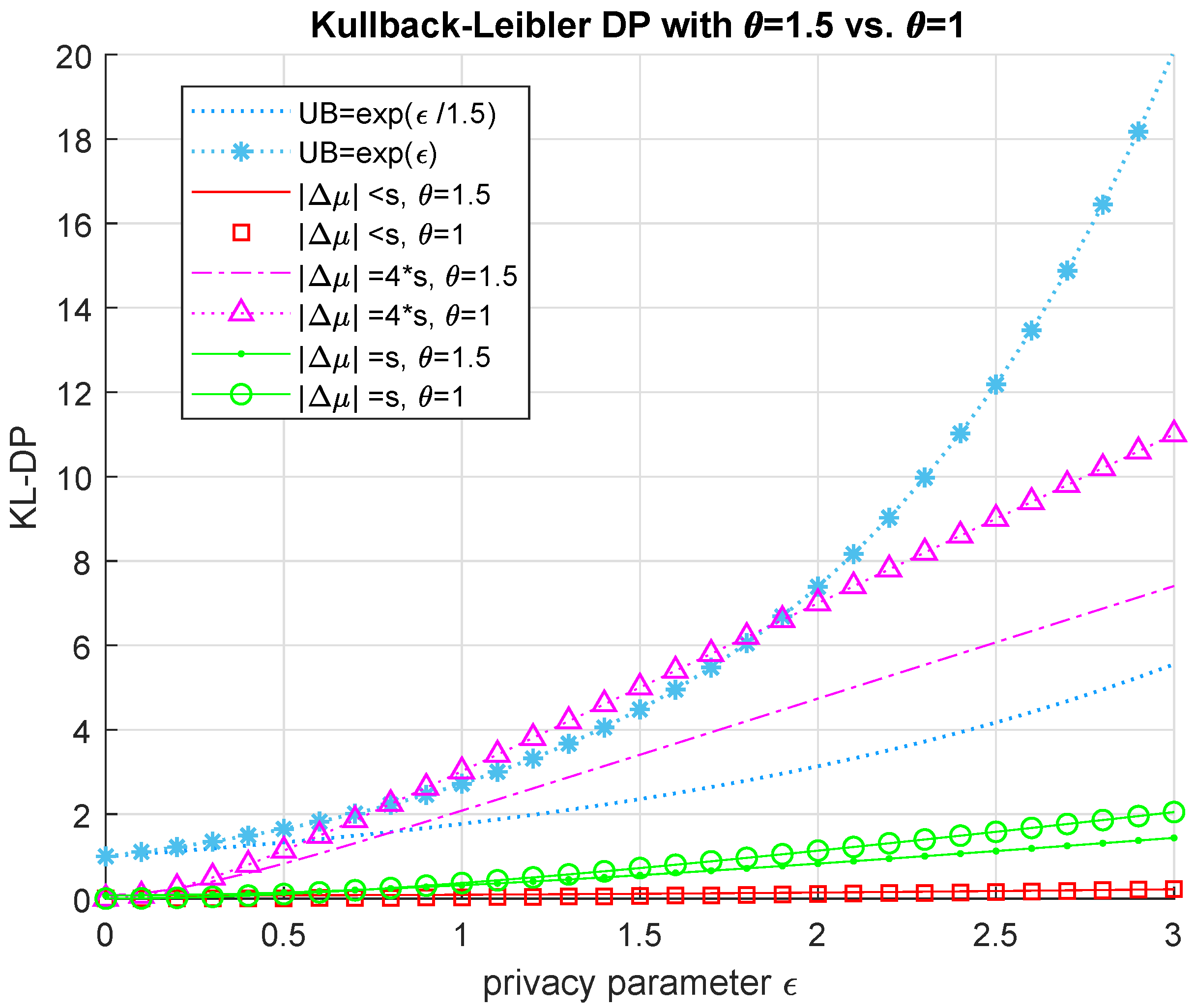[13] stands out in the way that the rate-distortion perspective is applied to DP, where various fidelity criteria is set to determine how fast the empirical distribution converges to the actual source distribution. We present an adaptation of the so-called Kullback–Leibler (KL)-DP [5] for detecting misclassification attacks in Laplace and Gaussian mechanisms, where the corresponding distributions in relative entropy were considered as the differentially private noise with and without the adversary’s advantage. Lastly, this work introduces a novel DP metric based on Chernoff information along with its application to adversarial classification.

Aside from statistical and information-theoretic approaches as employed in this paper, the literature on adversarial examples and attempts to correctly classify and detect them is rather rich. For instance, ref. [14] offers a game-theory-based risk analysis approach that was originally introduced by [15], whereas [16] introduce efficient algorithms for reverse engineering linear classifiers for adversarial classification. Adversarial classification dates back to [17], which assumes (somewhat unrealistically) that the adversary has the perfect knowledge of the classifier and attempt to detect these attacks by computation of the adversary’s optimal strategy. The novelty of the current paper lies in its methodology that makes use of information-theoretic quantities to solve a privacy and security problem.

1.2. Contributions and Outline

Our contributions are summarized in the following list.

• We consider a new attacker model whereby the adversary takes advantage of the underlying differentially private mechanism in order to remain undetected.
• We derive a trade-off between the privacy protected adversary’s advantage and the security of the system for the adversary to remain undetected while giving as much damage as possible to the system or, alternatively, for the defender to preserve the privacy of the system and detect the attacker. This trade-off is defined in the framework of statistical hypothesis testing similarly to [8].
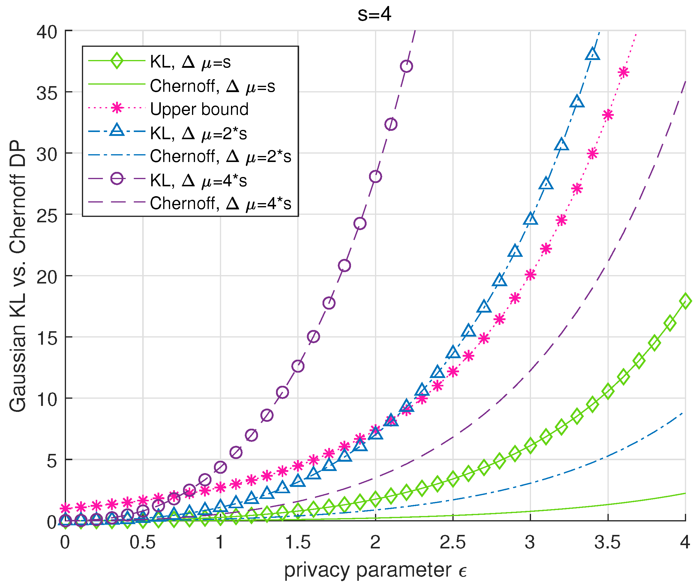
• We adopt the Kullback–Leibler DP definition of [5] to the addressed problem for adversarial classification in differentially private mechanisms and present numerical comparisons of different cases where the sensitivity of the system is less and greater than the bias induced by the adversary on the published information.
• We apply a source-coding approach to anomaly detection under differential privacy to bound the variance of the additional data by the sensitivity of the mechanism and the original data’s statistics by deriving the mutual information between the neighboring datasets.
• We introduce a new DP metric, that is called Chernoff DP, as a stronger alternative to the well-known $(ϵ,\delta )$-DP and KL-DP for the Gaussian mechanism. Chernoff DP is also adapted for adversarial classification and numerically shown to outperform KL-DP.

The outline of the paper is as follows. In the upcoming section, we remind the reader of some important preliminaries from the DP literature which will be used throughout this paper along with the detailed problem definition and performance criteria. In Section 3 and Section 4, we present statistical and information-theoretic thresholds for anomaly detection in Laplace and Gaussian mechanisms, respectively. Section 5 introduces divergence-based definitions of DP adapted for anomaly detection. We present numerical evaluation results in Section 6 and draw our final conclusions in Section 7.

2. System Model and Its Components

In this part, we revisit certain notions from the literature on DP which will also be employed in this paper. These preliminaries will be followed by a detailed definition of the addressed problem. We begin with defining the notion of neighborhood between datasets and sensitivity of DP.

Definition 1

(Neighboring datasets). Any two datasets that differ only in one row are called neighbors [4]. For two neighboring datasets, the following equality holds

$$d(x,\tilde{x})=1$$

(1)

where $d(.,.)$ denotes the Hamming (or $l_1$) distance between two datasets.

Definition 2

($L_1$ norm sensitivity [7]). Global sensitivity, denoted by s of a function (or a query) q: $D\to {\mathbb{R}}^k$ is the smallest possible upper bound on the distance between the images of q when applied to two neighboring datasets, i.e., the $l_1$ distance is bounded by $\parallel q\left(x\right)-q\left(\tilde{x}\right){\parallel }_1\le s$.

Basically, sensitivity of a DP mechanism is the smallest possible upper bound on the images of a query function for neighbors. Hence it is a function of the type of the query having an opposite relationship with the privacy. Higher sensitivity of the query refers to a stronger requirement for privacy guarantee, consequently more noise is needed to achieve that guarantee.

Definition 3

($(ϵ,\delta )$-DP [4]). A randomized algorithm $\mathcal{Y}$ is $(ϵ,\delta )$-differentially private if $\forall S\subseteq Range\left(\mathcal{Y}\right)$ and for all neighboring datasets x and $\tilde{x}$ within the domain of $\mathcal{Y}$ the following inequality holds.

$$Pr\left[\mathcal{Y}\left(x\right)\in S\right]\le Pr\left[\mathcal{Y}\left(\tilde{x}\right)\in S\right]exp\left\{ϵ\right\}+\delta$$

(2)

Next, we remind the reader of the Laplace distribution and Laplace mechanism. A differentially private system is named after the probability distribution of the perturbation applied onto the query output in the global setting. The Laplace distribution, also known as the double exponential distribution, is defined as

$$Lap(x;\mu ,b)=\frac{1}{2b}exp\left\{-\frac{|x-\mu |}{b}\right\}$$

(3)

with the location parameter equal to its mean $\mu \in \mathbb{R}$ and variance $2b^2$ where $b>0$ denotes the scale parameter.

Definition 4.

Laplace mechanism [7] is defined for a function (or a query) $q:D\to {\mathbb{R}}^k$ as follows

$$\mathcal{Y}(x,q(.),ϵ)=q\left(x\right)+(Z_1,\cdots ,Z_k)$$

(4)

where $Z_i\sim Lap(b=s/ϵ)$, $i=1,\cdots ,k$ denote i.i.d. Laplace random variables.

We will refer to the parameters $ϵ$ and $\delta$ as privacy budget throughout the paper. Next definition reminds the reader of the $L_2$ norm global sensitivity.

Definition 5.

$L_2$ norm sensitivity denoted s refers to the smallest possible upper bound on the $L_2$ distance between the images of a query $q:D\to {\mathbb{R}}^k$ when applied to two neighboring datasets $\mathbf{X}$ and $\tilde{\mathbf{X}}$ as

$$s=\underset{d(\mathbf{X},\tilde{\mathbf{X}})=1}{sup}\left|\right|q(\mathbf{X})-q(\tilde{\mathbf{X}}){\left|\right|}_2.$$

(5)

Definition 6.

Gaussian mechanism [7] is defined for a function (or a query) $q:D\to {\mathbb{R}}^k$ as follows

$$\mathcal{M}(\mathbf{X},q(.),ϵ,\delta )=q\left(\mathbf{X}\right)+(Z_1,\cdots ,Z_k)$$

(6)

where $Z_i\sim \mathcal{N}(0,{\sigma }^2)$, $i=1,\cdots ,k$ denote independent and identically distributed (i.i.d.) Gaussian random variables with the variance ${\sigma }_z^2=\frac{2s^{2}log(1.25/\delta )}{{ϵ}^2}$.

Theorem 1

([4]). The Laplace mechanism satisfies $(ϵ,0)$-differential privacy.

Theorem 2

([4]). For any $ϵ,\delta \in (0,1)$, the Gaussian mechanism satisfies $(\epsilon ,\delta )$-differential privacy.

Application of Gaussian noise results in a more relaxed privacy guarantee contrary to Laplace mechanism, which brings about $(ϵ,0)$-DP.

2.1. Problem Definition

Within the scope of this paper, we use two different approaches to study adversarial classification under differential privacy, namely the statistical approach to bound the first-order statistics of the additional data and an information-theoretic approach to characterize the second-order statistics of the attack. We define the original dataset in the following form $\mathbf{X}=X^n=\{X_1,\cdots ,X_n\}$. The query function takes the aggregation of this dataset as $q\left(\mathbf{X}\right)={\sum }_i^n{X}_i$ and the DP-mechanism adds Laplacian or Gaussian noise Z on the query output leading to the noisy output in the following form $\mathcal{M}(\mathbf{X},q(.),ϵ,\delta )=Y={\sum }_i^n{X}_i+Z$. This public information is altered by an adversary, who adds a single record denoted $X_a$ to this dataset. The modified output of the DP-mechanism becomes ${\sum }_i^n{X}_i+X_a+Z$. The reader should note that, we do not make any assumptions on the value of $X_a$.

2.1.1. First-Order Statistics of $X_a$

Our first approach is inspired by [8] where the authors determine statistical thresholds for the adversary’s hypothesis problem which is set to decide a given dataset entry is included in a dataset D or its neighbor $\tilde{D}$. This approach is adapted to the problem of detecting a strong adversary who does not only want to discover all the entries of a dataset but also wants to harm it. Accordingly, we set the following hypotheses where the null and alternative hypotheses are respectively translated into DP noise distribution with and without the bias induced by the attacker.

$$\begin{array}{cc}\hfill H_0& :\mathrm{defender}\mathrm{fails}\mathrm{to}\mathrm{detect}\mathrm{the}\mathrm{attack}\hfill \\ \hfill H_1& :\mathrm{defender}\mathrm{detects}\mathrm{the}\mathrm{attack}\hfill \end{array}$$

(7)

The hypothesis testing problem defined above in (7) can be translated into deciding on the DP noise distribution with its parameters. Here $H_0$ and $H_1$ correspond to DP noise following the probability distributions $p_0$ with mean ${\mu }_0$ and $p_1$ with mean ${\mu }_1$, respectively. Therefore, the decision boils down to choosing between $Y_0-{\sum }_{i=1}^n{X}_i=Z$ and $Y_0-\left[{\sum }_{i=1}^n{X}_i+X_a\right]$. Hence the shift in the location due to the addition of $X_a$ to the dataset is $\Delta \mu ={\mu }_1-{\mu }_0$. The corresponding likelihood ratio for this problem yields.

(8)

where $\mathcal{L}(.)$ denotes the likelihood function for the corresponding hypothesis and $\kappa$ is some positive number to be determined. Such a threshold defines the critical region in statistical hypothesis tests where the null hypothesis is rejected. This approach results in a precise trade-off between the attacker’s advantage (or the bias induced by the adversary) $\Delta \mu$, the sensitivity s and the privacy parameter $ϵ$ of the differentially private mechanism to characterize the threshold for rejecting the null hypothesis, i.e., detecting the attack, as a function of the error probabilities.

$\alpha$ and $\beta$ respectively denote type I and type II error probabilities which are defined for the hypothesis testing problem in (7) as follows:

$$\begin{array}{cc}\hfill P_{FA}=\alpha & =Pr\left[H_0\mathrm{reject}|H_0\mathrm{is}\mathrm{true}\right]\hfill \end{array}$$

(9)

$$\begin{array}{cc}\hfill P_{MD}=\beta & =Pr\left[H_1\mathrm{reject}|H_1\mathrm{is}\mathrm{true}\right].\hfill \end{array}$$

(10)

Based on the definition of $\alpha$, also called the probability of false-alarm, we denote its complement by $\overline{\alpha }=1-\alpha$. Similarly, due to (10), the complement of type II error probability (or the probability of mis-detection) is denoted by $\overline{\beta }=1-\beta$. The probability of detection $\overline{\beta }$ (i.e., correctly deciding $H_1$) is also called the power of the test in the statistics or the recall in machine learning terminology.

According to the Neyman–Pearson Theorem [18], the likelihood ratio compared against some positive integer defines the best critical region of size $\alpha$ for testing a simple hypothesis against an alternative simple hypothesis with the largest (or equally largest) power of the test. An extension of this result to testing against a composite alternative hypothesis is also possible. Such an extension is called uniformly most powerful test since such a test with the best critical region of size $\alpha$ is conducted for each possible value of the alternative hypothesis. Once we define the critical region for deciding between $H_0$ and $H_1$ in (7) as a function of $\Delta \mu$, the privacy parameter $ϵ$ and the sensitivity s, we will derive the error probabilities and the power of the test analytically as well as compute and depict them numerically.

2.1.2. Second-Order Statistics of $X_a$-Information-Theoretic Approach

Our second approach is inspired by rate-distortion theory. For Gaussian mechanism, we employ the biggest possible difference between the images of the query for the datasets with and without the additional data $X_a$ (i.e., neighboring inputs) as the fidelity criterion (Definition 5). Accordingly, we derive the mutual information between the original dataset and its neighbor in order to bound the additional data’s second-order statistics so that the defender fails to detect the attack. We assume that $X_a$ follows a normal distribution with the variance ${\sigma }_{X_a}^2$. To simplify our derivations, we also assume that the original dataset $X^n=\{X_1,X_2,\cdots ,X_i,\cdots ,X_n\}$ and its neighbor ${\tilde{X}}^n=\{X_1,X_2,\cdots ,X_i,\cdots ,X_n+X_a\}$ have the same dimension n. Alternatively, the attack would change the size of the dataset as $n+1$ where the additional data are not added to either of the $X_i$’s.

3. Adversarial Classification in Laplace Mechanisms

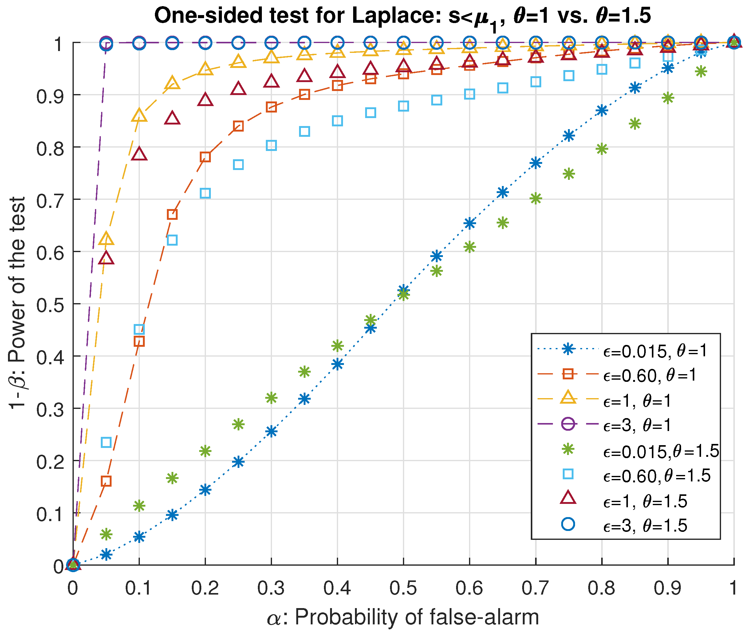
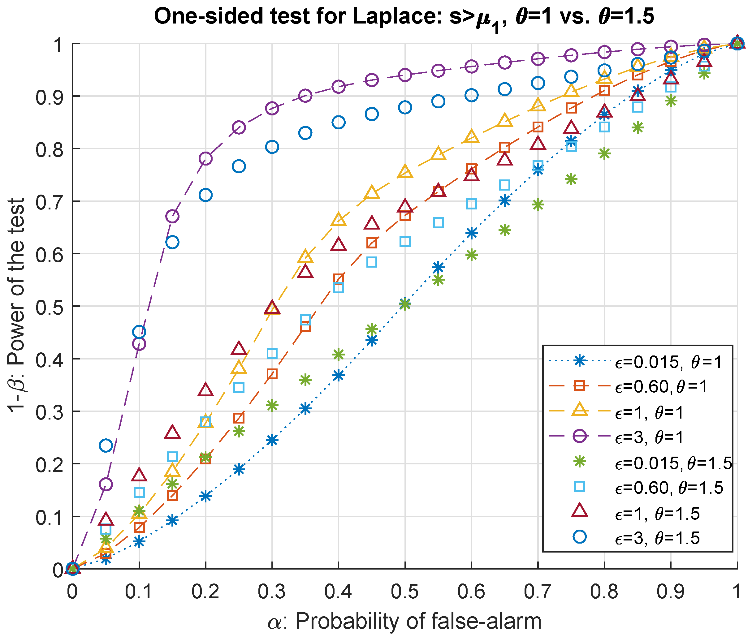
We separate our results in two main groups for $(ϵ,0)$-DP in Laplace mechanisms for one-sided and two-sided hypothesis tests.

• One-Sided Test

We will investigate both cases of setting the alternative hypothesis $H_1$ as either ${\mu }_1>{\mu }_0$ (i.e., $\Delta \mu >0$) or ${\mu }_1<{\mu }_0$ (i.e., $\Delta \mu <0$). This corresponds to a one-sided hypothesis testing problem. The decision of choosing between the hypotheses in (7) boils down to deciding between $Y_0-{\sum }_{i=1}^n{X}_i=Z\sim Lap(z;{\mu }_0,s/ϵ)$ and $Y_0-\left[{\sum }_{i=1}^n{X}_i+X_a\right]=Z\sim Lap(z;{\mu }_1,\theta (s/ϵ))$ where $\theta \ge 1$ as the measure of the change in the privacy budget of the system whereas s and $ϵ$ denote the sensitivity and privacy parameter, respectively. It should be noted that setting $\theta =1$ translates the hypothesis test in (7) into testing only the location parameter of the Laplacian DP noise. Our goal is to derive a relationship between the privacy parameter, the significance level (or the probability of false alarm), type II error probability (or the probability of mis-detection) for the attacker to be successful, i.e., to fail to reject $H_0$, as a function of the bias $\Delta \mu$. The corresponding likelihood ratio to (7) is given by

(11)

where $\kappa$ is some positive number to be determined and $({\mu }_i,b_i)$ for $i=0,1$ represent the location and scale parameters of the distributions to be tested.

The next theorem states our first main result which presents a threshold of correctly detecting the adversary for a given level of privacy budget, sensitivity and type I error probability.

Theorem 3.

The threshold of the best critical region of size α defined in (9) for deciding between the null hypothesis and its alternative of the one-sided hypothesis testing problem in (7) for a Laplace mechanism with the largest power $\overline{\beta }$ is given as a function of the probability of false alarm α, privacy parameter ϵ and global sensitivity s as follows

$$k=\left\{\begin{array}{cc}{\mu }_0+\frac{s}{ϵ}ln\left(2(1-\alpha )\right)\hfill & if\alpha \in [0,0.5]\hfill \\ {\mu }_0-\frac{s}{ϵ}ln\left(2\alpha \right)\hfill & if\alpha \in [0.5,1]\hfill \end{array}\right.$$

(12)

Then according to the adversary’s hypothesis testing problem, the defender detects the attack for $\Delta \mu >0$ if the output of the Laplace mechanism $Y_0$ exceeds $(k+q(x\left)\right)$ where $q(.)$ is the noiseless query output. Similarly, for $\Delta \mu <0$, the attack is detected if $Y_0<q\left(x\right)+k$.

Remark 1.

The decision rule given by Theorem 3 is equivalent to comparing the Laplace noise to the threshold k as it will be shown by the following proof. For positive bias, the critical region becomes $(k,\infty )$ thus, . By analogy if $\Delta \mu <0$, the critical region for the Laplace noise becomes $(-\infty ,k)$.

Proof. 

According to the Neyman–Pearson theorem [18], each point where $\Lambda \ge \kappa$ composes the best critical region of size α as defined in (9) for this simple hypothesis testing problem. Using the ratio in (11), we will determine the threshold k as a function of the best critical region, the power of the test, the privacy budget and lastly, the attack.

We expand Λ as follows.

$$\begin{array}{cc}\hfill \Lambda & =\frac{\frac{1}{2\theta (s/ϵ)}exp\left\{-\frac{|z-{\mu }_1|}{\theta (s/ϵ)}\right\}}{\frac{1}{2s/ϵ}exp\left\{-\frac{|z-{\mu }_0|}{s/ϵ}\right\}}\hfill \end{array}$$

(13)

$$\begin{array}{cc}\hfill & =\frac{1}{\theta }exp\left\{\frac{ϵ|z-{\mu }_0|}{s}-\frac{ϵ|z-{\mu }_1|}{\theta s}\right\}\hfill \end{array}$$

(14)

The likelihood ratio in (13) can be summarized by the following piecewise function based on the possible relationships between ${\mu }_1$ and z due to the absolute value in the exponent of the probability distribution for ${\mu }_1<{\mu }_0$.

$${\Lambda }_I=\left\{\begin{array}{cc}\frac{1}{\theta }exp\left\{\frac{ϵ}{\theta s}\left(z(1-\theta )+\theta {\mu }_0-{\mu }_1\right)\right\}\hfill & \mathrm{if}z<{\mu }_1\hfill \\ \frac{1}{\theta }exp\left\{-\frac{ϵ}{\theta s}(z(1+\theta )-\theta {\mu }_0-{\mu }_1)\right\}\hfill & \mathrm{if}z\in [{\mu }_1,{\mu }_0]\hfill \\ \frac{1}{\theta }exp\left\{-\frac{ϵ}{\theta s}(z(1-\theta )+\theta {\mu }_0-{\mu }_1)\right\}\hfill & \mathrm{if}z\ge {\mu }_0\hfill \end{array}\right.$$

(15)

Equivalently, ${\Lambda }_I$ is confined in the interval

$$\left[\frac{1}{\theta }exp\left\{-\frac{ϵ}{\theta s}\left(z(1-\theta )+\theta {\mu }_0-{\mu }_1\right)\right\},\frac{1}{\theta }exp\left\{\frac{ϵ}{\theta s}\left(z(1-\theta )+\theta {\mu }_0-{\mu }_1\right)\right\}\right].$$

On the other hand, for ${\mu }_1>{\mu }_0$, the corresponding likelihood ratio for the hypotheses in (7) yields

$${\Lambda }_{II}=\left\{\begin{array}{cc}\frac{1}{\theta }exp\left\{\frac{ϵ}{\theta s}(z(1-\theta )+\theta {\mu }_0-{\mu }_1)\right\}\hfill & \mathrm{if}z<{\mu }_0\hfill \\ \frac{1}{\theta }exp\left\{\frac{ϵ}{\theta s}(z(1+\theta )-\theta {\mu }_0-{\mu }_1)\right\}\hfill & \mathrm{if}z\in [{\mu }_0,{\mu }_1]\hfill \\ \frac{1}{\theta }exp\left\{-\frac{ϵ}{\theta s}(z(1-\theta )+\theta {\mu }_0-{\mu }_1)\right\}\hfill & \mathrm{if}z\ge {\mu }_1\hfill \end{array}\right.$$

(16)

To be able to determine a threshold for deciding between the hypotheses in (7), we compute the false alarm rate α and the mis-detection error β (and the power of the test, that is $1-\beta$) applying the Neyman–Pearson lemma that guarantees maximizing the power of the hypothesis test for a given false alarm rate α.

• Derivation of $\alpha$:

Based on the definition in (9), for $\Delta \mu >0$ the probability of raising a false-alarm is derived by integrating the following probability distribution over the critical region

$$\begin{array}{cc}\hfill \alpha & =Pr\left[H_0\mathrm{reject}\right|H_0\mathrm{is}\mathrm{true}]\hfill \end{array}$$

(17)

$$\begin{array}{cc}\hfill & ={\int }_k^{\infty }\frac{ϵ}{2s}exp\left\{-\frac{ϵ|z-{\mu }_0|}{s}\right\}dz,\hfill \end{array}$$

(18)

which is further expanded out in two possible ways. First for $k<{\mu }_0$, we get

$$\begin{array}{cc}\hfill \alpha & =1-{\int }_{-\infty }^k\frac{ϵ}{2s}exp\left\{\frac{ϵ}{s}(z-{\mu }_0)\right\}dz\hfill \end{array}$$

(19)

$$\begin{array}{cc}\hfill & =1-\frac{1}{2}exp\left\{\frac{ϵ}{s}(k-{\mu }_0)\right\}\hfill \end{array}$$

(20)

Second, we have for $k\ge {\mu }_0$

$$\begin{array}{cc}\hfill \alpha & ={\int }_k^{\infty }\frac{ϵ}{2s}exp\left\{-\frac{ϵ}{s}(z-{\mu }_0)\right\}dz\hfill \end{array}$$

(21)

$$\begin{array}{cc}\hfill & =\frac{1}{2}exp\left\{-\frac{ϵ}{s}(k-{\mu }_0)\right\}\hfill \end{array}$$

(22)

Rewriting (20) and (22) as an equality for k, we obtain the piecewise function (12) as the threshold in Theorem 3 as a function of α. If the bias induced by the adversary is negative, i.e., $\Delta \mu <0$, then the conditions to obtain (20) and (22) are swapped. For $\Delta \mu <0$ and $k<{\mu }_0$, we get (22) for the probability of false-alarm.

• How to determine $\kappa$?:

According to the piecewise expansions of likelihood ratio functions in (16) and (15) respectively for $\Delta \mu <0$ and $\Delta \mu >0$, we have the intervals for κ given by (23) and (24) on top of the next page since .

$$\begin{array}{cc}\hfill \frac{1}{\theta }exp\left\{-\frac{ϵ}{\theta s}(z(1-\theta )+\theta {\mu }_0-{\mu }_1\right\}& <\kappa <\frac{1}{\theta }exp\left\{\frac{ϵ}{\theta s}\left(z(1-\theta )+\theta {\mu }_0-{\mu }_1\right)\right\},\mathrm{for}\Delta \mu <0\hfill \end{array}$$

(23)

$$\begin{array}{cc}\hfill \frac{1}{\theta }exp\left\{\frac{ϵ}{\theta s}(z(1-\theta )+\theta {\mu }_0-{\mu }_1)\right\}& <\kappa <\frac{1}{\theta }exp\left\{-\frac{ϵ}{\theta s}(z(1-\theta )+\theta {\mu }_0-{\mu }_1)\right\},\mathrm{for}\Delta \mu >0\hfill \end{array}$$

(24)

Therefore, the null hypothesis is rejected for

$$\frac{1}{\theta }exp\left\{-\frac{ϵ}{\theta s}(z(1+\theta )-\theta {\mu }_0-{\mu }_1)\right\}<\kappa \mathrm{for}\Delta \mu <0$$

(25)

or

$$\frac{1}{\theta }exp\left\{\frac{ϵ}{\theta s}(z(1+\theta )-\theta {\mu }_0-{\mu }_1)\right\}>\kappa \mathrm{for}\Delta \mu >0$$

(26)

Due to the threshold of the critical region defined in Theorem 3, we finally get κ as follows

$$\begin{array}{cc}\hfill \kappa & =\frac{1}{\theta }exp\left\{-\frac{ϵ}{\theta s}(k(1+\theta )-\theta {\mu }_0-{\mu }_1)\right\}\mathrm{for}\Delta \mu <0\hfill \end{array}$$

(27)

$$\begin{array}{cc}\hfill \kappa & =\frac{1}{\theta }exp\left\{\frac{ϵ}{\theta s}(k(1+\theta )-\theta {\mu }_0-{\mu }_1)\right\}\mathrm{for}\Delta \mu >0\hfill \end{array}$$

(28)

□

• Derivation of the power of the test:

The power of the hypothesis test is the probability of rejecting the null hypothesis $H_0$ given that the alternative hypothesis $H_1$ is true. Let $\overline{\beta }$ denote the complement of the type II error β, we have using the definition in (10) for $\Delta \mu >0$ and $k<{\mu }_1$

$$\begin{array}{cc}\hfill \overline{\beta }& =1-Pr\left[H_1\mathrm{reject}|H_1\mathrm{is}\mathrm{true}\right]\hfill \end{array}$$

(29)

$$\begin{array}{cc}\hfill & ={\int }_k^{\infty }\frac{ϵ}{2\theta s}exp\left\{\frac{ϵ({\mu }_1-z)}{\theta s}\right\}dz\hfill \end{array}$$

(30)

$$\begin{array}{cc}\hfill & =\frac{1}{2}exp\left\{\frac{ϵ({\mu }_1-k)}{\theta s}\right\}\hfill \end{array}$$

(31)

As for $k>{\mu }_1$, the power function becomes

$$\begin{array}{cc}\hfill \overline{\beta }& =1-{\int }_{-\infty }^k\frac{ϵ}{2\theta s}exp\left\{\frac{ϵ(z-{\mu }_1)}{\theta s}\right\}dz\hfill \end{array}$$

(32)

$$\begin{array}{cc}\hfill & =1-\frac{1}{2}exp\left\{\frac{ϵ(k-{\mu }_1)}{\theta s}\right\}\hfill \end{array}$$

(33)

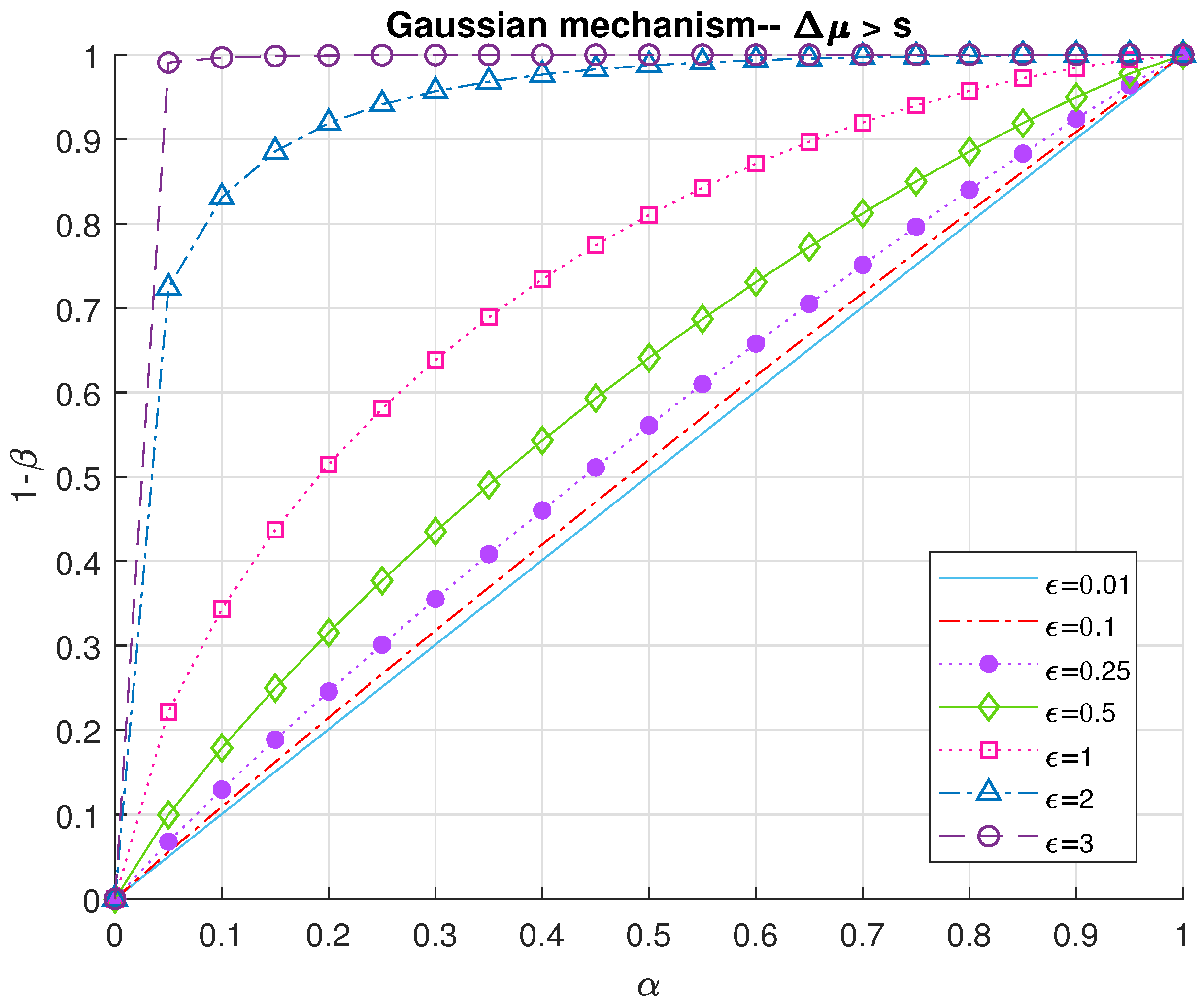
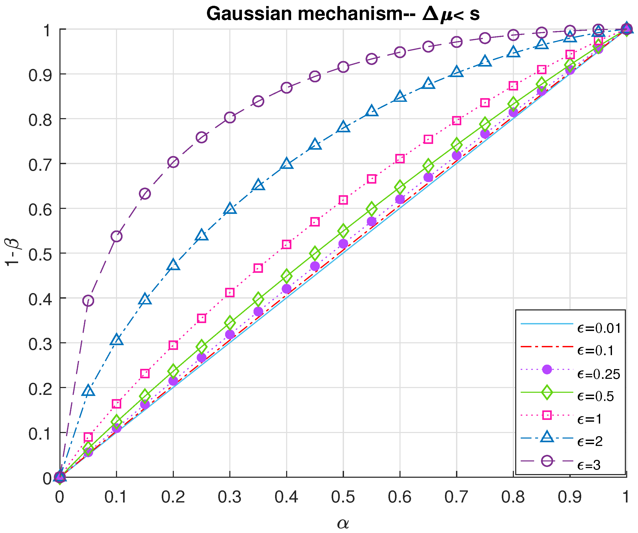
On the contrary for negative bias $\Delta \mu <0$, the conditions based on k and ${\mu }_1$ to obtain (29) and (32) are swapped. In Section 6, we present numerical evaluation results for Theorem 3 using the probability of false-alarm $P_{FA}$ and power of the test $1-P_{MD}=\overline{\beta }$ to draw receiving operating characteristic curves (ROC) as performance analysis.

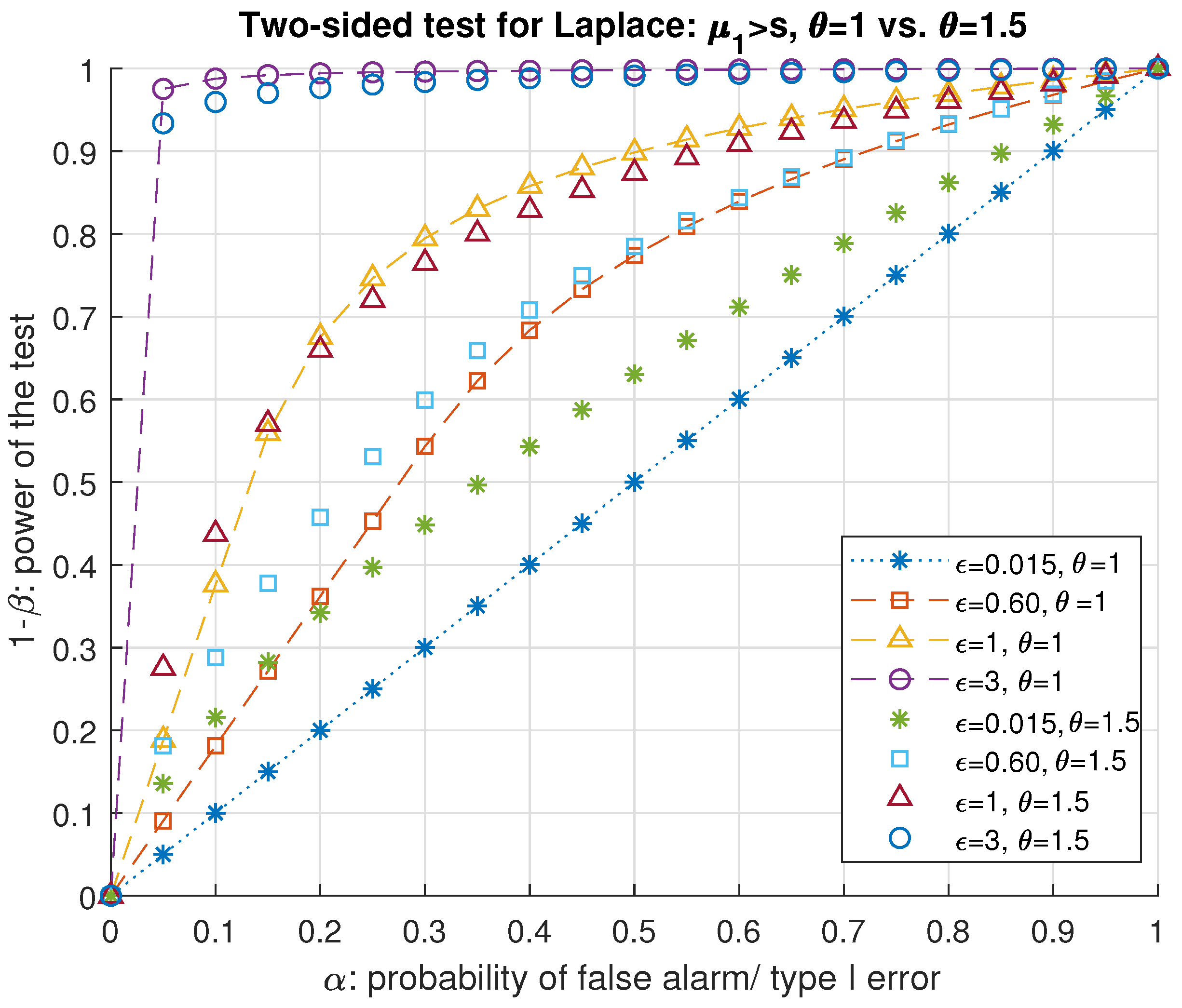
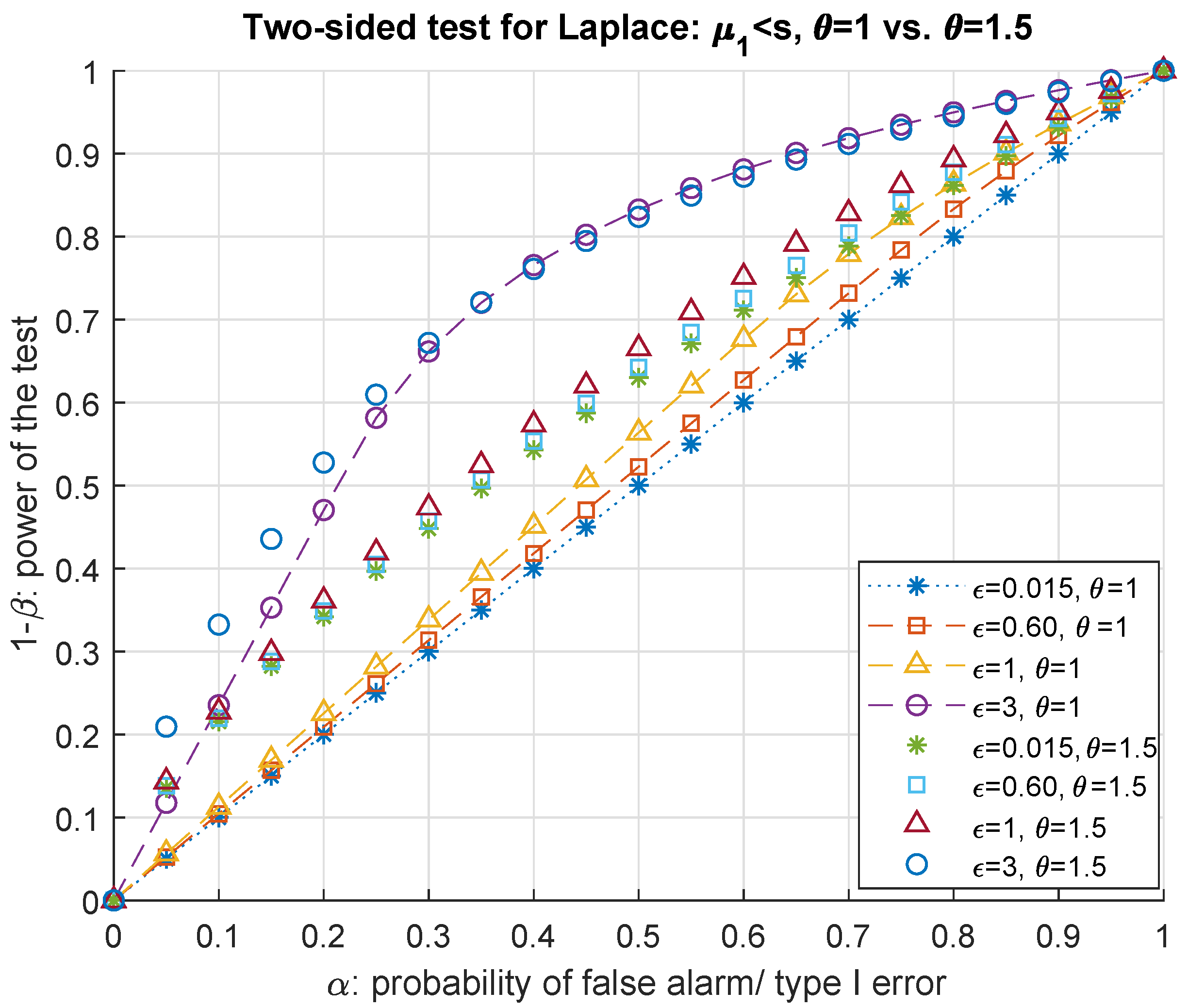
Remark 2.

Special case of $\theta =1$ and $|\Delta {\mu }_1|\le s$: Setting $\theta =1$ in (13), it can be easily observed that both likelihood ratios ${\Lambda }_I$ in (15) and ${\Lambda }_{II}$ in (16) are included in the following interval $[exp\left\{-\Delta \mu \frac{ϵ}{s}\right\},exp\left\{\Delta \mu \frac{ϵ}{s}\right\}]$. Applying also $|\Delta {\mu }_1|\le s$ onto the likelihood ratio Λ in (13), we get $exp\{-ϵ\}\le \Lambda \le exp\left\{ϵ\right\}$ which is the $(ϵ,0)$-DP.

3.1. Two-Sided Test

As an alternative solution to the same problem of detecting the attacker through determining the shifts and changes in the location and deviation of the DP noise using a one-sided hypothesis test, a two-sided test could provide a more realistic solution where it is not possible to assume the direction of the shift induced by the adversary. Hence the hypothesis test in (7) can be conducted for determining the (possible) change in the distribution of the DP noise in both directions where the null hypothesis remains the same as $H_0:Z\sim Lap({\mu }_0,s/ϵ)$ to test against the alternative $H_1:Z\sim Lap({\mu }_1,\theta s/ϵ)$.

This translates to choosing between

$$\begin{array}{cc}\hfill H_0& :\mu ={\mu }_0,b=s/ϵ\hfill \end{array}$$

(34)

$$\begin{array}{cc}\hfill H_1& :\mathrm{at}\mathrm{least}\mathrm{one}\mathrm{of}\mathrm{the}\mathrm{equalities}\mathrm{does}\mathrm{not}\mathrm{hold}\hfill \end{array}$$

(35)

where μ denotes the location parameter and b denoted the scale parameter of any Laplace distribution. The alternative hypothesis can also be stated with the parameters $\mu ={\mu }_1$, $b=\theta s/ϵ$ where $\theta \ge 1$.

In this two-sided test, there are two thresholds on each side of the origin to be determined for the critical region each with a size of $\alpha /2$. Let $k_1$ and $k_2$ denote the threshold greater and smaller than the origin, respectively. The next theorem presents the thresholds for detecting the attack as a function of the probability of false-alarm and the privacy budget of the differentially private mechanism as its one-sided counterpart given by Theorem 3.

Theorem 4.

The threshold of the best critical region of size α defined in (9) for choosing between the null hypothesis and its alternative of the two-sided hypothesis testing problem in (34) and (35) for a Laplace mechanism with the largest power $\overline{\beta }$ is

$$\begin{array}{ccc}\hfill k_1& =& {\mu }_0-(s/ϵ)log\alpha \hfill \end{array}$$

(36)

$$\begin{array}{ccc}\hfill k_2& =& {\mu }_0+(s/ϵ)log\alpha \hfill \end{array}$$

(37)

Then according to the adversary’s hypothesis testing problem, the defender fails to detect the attack when the output of the Laplace mechanism $Y_0$ is confined in $(q\left(x\right)+k_2,q\left(x\right)+k_1)$ where $q(.)$ is the noiseless query output.

Proof. 

The null hypothesis cannot be rejected if the noisy output of the Laplace mechanism is confined in the interval $(k_2,k_1)$. First, we begin with the derivation of threshold for the output of the DP mechanism. The probability of raising a false-alarm or having a type I error is derived as follows.

$$\begin{array}{cc}\hfill \alpha & =Pr\left[H_0\mathrm{reject}\right|H_0\mathrm{is}\mathrm{true}]\hfill \end{array}$$

(38)

$$\begin{array}{cc}\hfill & ={\int }_{-\infty }^{k_2}\frac{ϵ}{2s}exp\left\{\frac{ϵ(z-{\mu }_0)}{s}\right\}dz+{\int }_{k_1}^{\infty }\frac{ϵ}{2s}exp\left\{-\frac{ϵ(z-{\mu }_0)}{s}\right\}dz\hfill \end{array}$$

(39)

Each addend of α corresponds to one half of the probability of false-alarm. Equating each integral to $\alpha /2$ and rewriting the equalities in terms of $k_1$ and $k_2$, we get the thresholds in (37). □

3.2. A Trade-off between ${\mu }_1$, s and $ϵ$ for Detecting the Attacker-Two-Sided Test

Using the threshold presented in Theorem 4, we can determine an interval to confine the mean of the attacker’s advantage to be detected by the DP mechanism, i.e., for the null hypothesis $H_0$ to be rejected. Alternatively, such an interval can be converted for the privacy parameter ϵ as a function of error probabilities, the attack and the sensitivity. The following result, Corollary 1, presents upper and lower bounds on the attacker’s advantage so that the defender detects the attack.

There are two possible cases w.r.t. the relationship between ${\mu }_0$ and ${\mu }_1$. The alternative hypothesis in this two-sided test also states that these two parameters are unequal. As we have discussed earlier in the derivation of the threshold for determining the critical region in Laplace mechanisms, whether ${\mu }_0>{\mu }_1$ or ${\mu }_1>{\mu }_0$ directly effects the likelihood ratio function, and thus the condition to reject the null hypothesis. Let us then consider the first possible case of ${\mu }_0<{\mu }_1$. In this case, we have either $k_2<{\mu }_0<k_1<{\mu }_1$ or $k_2<{\mu }_0<{\mu }_1<k_1$. On the contrary for ${\mu }_1<{\mu }_0$, we have for the thresholds either of the cases ${\mu }_1<k_2<{\mu }_0<k_1$ or $k_2<{\mu }_1<{\mu }_0<k_1$. These different cases can be used for deriving an interval to include $\Delta \mu$ as a function of the error probabilities, privacy budget and the sensitivity.

Corollary 1.

The absolute bias $|\Delta \mu |=|{\mu }_1-{\mu }_0|$ induced by the adversary is confined in the following interval so that the defender detects $X_a$ and preserves $(ϵ,0)$- DP

$$\frac{s}{ϵ}log\left(\alpha {\overline{\beta }}^{\theta }\right)<\Delta \mu <\frac{s}{ϵ}log\left(\frac{1}{\alpha {\overline{\beta }}^{\theta }}\right)$$

(40)

for $\theta \ge 1$ where α and $\overline{\beta }$ respectively are the significance level and the power of the test of (35).

Proof. 

We begin with deriving the power of the two-sided test (35) as a function of the thresholds of the critical region. The probability of correctly detecting the attacker is as follows.

$$\begin{array}{cc}\hfill \overline{\beta }& ={\int }_{-\infty }^{k_2}\frac{ϵ}{2\theta s}exp\left\{\frac{ϵ(z-{\mu }_1)}{\theta s}\right\}dz+{\int }_{k_1}^{\infty }\frac{ϵ}{2\theta s}exp\left\{-\frac{ϵ(z-{\mu }_1)}{\theta s}\right\}dz\hfill \end{array}$$

(41)

$$\begin{array}{cc}\hfill & =\frac{1}{2}exp\left\{\frac{ϵ(k_2-{\mu }_1)}{\theta s}\right\}+\frac{1}{2}exp\left\{-\frac{ϵ(k_1-{\mu }_1)}{\theta s}\right\}\hfill \end{array}$$

(42)

Each addend in (41) corresponds to $\overline{\beta }/2$ and can be rewritten for the thresholds as functions of the power of the test as $k_1={\mu }_1-\frac{s}{ϵ}log{\left(\overline{\beta }\right)}^{\theta }$ and $k_2={\mu }_1+\frac{s}{ϵ}log{\left(\overline{\beta }\right)}^{\theta }$. Combining this with $k_2<k_1$ for the case ${\mu }_0<{\mu }_1$, the bias is lower bounded as follows

$$\begin{array}{cc}\hfill {\mu }_0+\frac{s}{ϵ}log\alpha & <{\mu }_1-\frac{\theta s}{ϵ}log\overline{\beta }\hfill \end{array}$$

(43)

$$\begin{array}{cc}\hfill \frac{s}{ϵ}log\left(\alpha {\overline{\beta }}^{\theta }\right)& <\Delta \mu \hfill \end{array}$$

(44)

As for the upper bound we have

$$\begin{array}{cc}\hfill {\mu }_1+\frac{\theta s}{ϵ}log\overline{\beta }& <{\mu }_0-\frac{s}{ϵ}log\alpha \hfill \end{array}$$

(45)

$$\begin{array}{cc}\hfill \Delta \mu & <\frac{s}{ϵ}log\left(\frac{1}{\alpha {\overline{\beta }}^{\theta }}\right)\hfill \end{array}$$

(46)

By analogy, we get the swapped upper and lower bound for $-\Delta \mu$ for the second case of ${\mu }_1<{\mu }_0$. Finally, we get the interval for the absolute bias as given by (40). This concludes the proof of the corollary. □

4. Adversarial Classification in Gaussian Mechanisms

Next, we apply a source-coding approach to anomaly detection under DP, which results in an upper bound on the variance of the additional data $X_a$ as a function of the sensitivity of the mechanism and the original data’s statistics. Additionally, we present a statistical trade-off between the probability of false alarm, privacy budget and the impact of the attack for the first-order statistics of the data in Section 4.2.

4.1. Privacy-Distortion Trade-off for Second-Order Statistics

The idea applied here is to render the problem of adversarial classification under DP as a lossy source-coding problem. Instead of using the mutual information between the input and output (or the input’s estimate obtained via the output), considering the adversary’s conflicting goals we derive the mutual information between the datasets before and after the attack. We present the main result for Gaussian mechanism by the following theorem.

Theorem 5.

The privacy-distortion function for a dataset $X^n$ and Gaussian mechanism as defined by (6) is

$$P\left(s\right)=\frac{1}{2}log\left(f_n\left(1+\prod _i^n{\sigma }_{X_i}^2/s^2\right)\right),$$

(47)

for $s\in \left[0,{\prod }_i^n{\sigma }_{X_i}^2\right]$ and zero elsewhere. ${\sigma }_{X_i}$ denotes the standard deviation of $X_i$ for $i=1,\cdots ,n$, $f_n$ is some constant dependent on the size of the dataset n and ${\sigma }_{X_i}$ is the standard deviation of the additional data.

Proof. 

The first expansion of $I(X^n;{\tilde{X}}^n)$ proceeds as follows

$$\begin{array}{cc}\hfill & I(X^n;{\tilde{X}}^n)=h(X^n)-h(X^n|{\tilde{X}}^n)\hfill \end{array}$$

(48)

$$\begin{array}{cc}\hfill & \ge h(X^n)-h(q(X^n)-{\tilde{X}}^n|{\tilde{X}}^n)\hfill \end{array}$$

(49)

$$\begin{array}{cc}\hfill & =h(X^n)-h(q(X^n)-q({\tilde{X}}^n)|{\tilde{X}}^n)\hfill \end{array}$$

(50)

$$\begin{array}{cc}\hfill & \ge h(X^n)-h(q(X^n)-q({\tilde{X}}^n))\hfill \end{array}$$

(51)

$$\begin{array}{cc}\hfill & \ge \frac{1}{2}\sum _{i=1}^{n}log\left(\left(2\pi \mathrm{e}\right){\sigma }_{X_i}^2\right)-\frac{1}{2}log\left(2\pi \mathrm{e}{s}^2\right)\hfill \end{array}$$

(52)

$$\begin{array}{cc}\hfill & =\frac{1}{2}log\left({(2\pi \mathrm{e})}^{n-1}\prod _i^n{\sigma }_{X_i}^2/s^2\right)\hfill \end{array}$$

(53)

In (51), we apply the following property due to concavity of entropy function, $h(g(x))\le h(x)$ for any function $g(.)$ and introduce the lower bound since the condition conditioning reduces entropy. In (52), we plug in Definition 5 into the second term after bounding it by Gaussian entropy. □

It is worth noting that the additional factor $2\pi \mathrm{e}$ appears here as opposed to the original rate-distortion function due to the choice of the query function that aggregates the entire dataset and returns an output of size 1.

Corollary 2.

The second order statistics of the additional data inserted into the dataset by the adversary is upper bounded by a function of the privacy budget $(ϵ,\delta )-$ and the statistics of the original dataset as follows

$${\sigma }_{X_a}^2\le \frac{1}{{(2\pi \mathrm{e})}^{n-1}}\left[\frac{s^2}{1-s^2/{\sigma }_{X_n}^2}\right]$$

(54)

where $s^2=\frac{{\sigma }_z^2{ϵ}^2}{2log(1.25/\delta )}$ due to Definition 6 for $n\ge 2$.

Proof. 

For the second expansion of $I(X^n;{\tilde{X}}^n)$, we have the following considering the neighbor that includes $X_a$ has now $(n+1)$ entries over n rows as ${\tilde{X}}^n=\{X_1,X_2,\cdots ,X_n+X_a\}$.

$$\begin{array}{cc}\hfill & I(X^n;{\tilde{X}}^n)=h({\tilde{X}}^n)-h({\tilde{X}}^n|X^n)\hfill \end{array}$$

(55)

$$\begin{array}{cc}\hfill & \le \sum _{i=1}^n\frac{1}{2}log{\left(2\pi \mathrm{e}\right)}^n{\sigma }_{X_i}^2-\frac{1}{2}log\left({(2\pi \mathrm{e})}^n{\sigma }_{X_a}^2\right)\hfill \end{array}$$

(56)

$$\begin{array}{cc}\hfill & =\frac{1}{2}log\left({(2\pi \mathrm{e})}^n\prod _{i=1}^{n-1}{\sigma }_{X_i}^2({\sigma }_{X_n}^2+{\sigma }_{X_a}^2)\right)-\frac{1}{2}log\left({(2\pi \mathrm{e})}^n{\sigma }_{X_a}^2\right)\hfill \end{array}$$

(57)

$$\begin{array}{cc}\hfill & =\frac{1}{2}log\prod _{i=1}^{n-1}{\sigma }_{X_i}^2\left(1+\frac{{\sigma }_{X_n}^2}{{\sigma }_{X_a}^2}\right)\hfill \end{array}$$

(58)

Due to the adversary’s attack, in the first term of (56), we add up the variances of $(n+1)$ $X_i$’s including $X_a$. Since (58) ≥ (53), global sensitivity is bounded as follows in terms of the second-order statistics of the original data and those of the additional data $X_a$.

$$s\ge {(2\pi \mathrm{e})}^{\frac{n-1}{2}}\frac{{\sigma }_{X_n}·{\sigma }_{X_a}}{{\left({\sigma }_{X_n}^2+{\sigma }_{X_a}^2\right)}^{1/2}}$$

(59)

Alternatively, the lower bound on the sensitivity of the Gaussian mechanism can be used as an upper bound on ${\sigma }_{X_a}^2$ to yield a threshold in terms of the additional data $X_a$’s variance as a function of the privacy budget and the original data $X_n$’s statistics to guarantee that the adversary avoids being detected. □

Remark 3.

The second expansion of the mutual information between neighboring datasets derived in (53), can be related to the well-knownrate-distortion function of the Gaussian sourcewhich, originally, provides the minimum possible transmission rate for a given distortion balancing (mostly for the Gaussian case) the squared-error distortion with the source variance. This is in line with the adversary’s goal in our setting, where the adversary aims to maximize the damage that s/he inflicts on the DP-mechanism. However, at the same time, to avoid being detected the attack is calibrated according to the sensitivity which here replaces the distortion. Thus, similar to the classical rate-distortion theory, here the mutual information between the neighbors is minimized for a given sensitivity to simultaneously satisfy adversary’s conflicting goals for the problem of adversarial classification under Gaussian DP-mechanism.

4.2. A Statistical Threshold-First-Order Statistics

Next, we present a statistical trade-off between the privacy budget of the Gaussian mechanism and the adversary’s advantage.

Theorem 6.

The adversary avoids being correctly detected by the defender with the largest possible power of the test $\overline{\beta }=1-\beta$ and the best critical region of size $\alpha =1-\overline{\alpha }$ for positive bias, if the following inequality holds

$$\Delta \mu \le \left(Q^{-1}(\alpha )-Q^{-1}(\overline{\beta })\right){\sigma }_z$$

(60)

where $Q(.)$ denotes the Gaussian Q-function defined as $Pr[T>t]$ and for ${\sigma }_z=\frac{\sqrt{2}·s·.5·log(1.25/\delta )}{ϵ}$. By analogy, for negative bias, we have

$$\Delta \mu \ge \left(Q^{-1}(\overline{\alpha })-Q^{-1}(\beta )\right){\sigma }_Z$$

(61)

Proof. 

Likelihood ratio function Λ to choose between $Y-{\sum }_i^n{X}_i$ and $Y-{\sum }_i^n{X}_i-X_a$ results in $z>\tilde{k}$ where $\tilde{k}=\frac{{\sigma }_z^{2}logk}{\Delta \mu }+\frac{{\mu }_1+{\mu }_0}{2}$ by setting $p_0$ and $p_1$ as Gaussian distributions with respective location parameters ${\mu }_0$ and ${\mu }_1$ and the mutual scale parameter ${\sigma }_z$. Probability of rejecting $H_0$ in case of an attack is derived using this condition as

$$\alpha =\left\{\begin{array}{c}Q\left(\frac{{\sigma }_{z}logk}{\Delta \mu }+\frac{\Delta \mu }{2{\sigma }_z}\right)\Delta \mu >0,\hfill \\ 1-Q\left(\frac{{\sigma }_{z}logk}{\Delta \mu }+\Delta \mu /(2{\sigma }_z)\right)\hfill \end{array}\right.$$

(62)

where $Q(.)$ denotes the Gaussian Q-function defined as $Pr[T>t]$ for standard Gaussian random variables. The threshold of the critical region k for $\Delta \mu >0$ is obtained as a function of the probability of false-alarm as $k=exp\left\{\frac{\Delta \mu }{{\sigma }_z}\left(Q^{-1}(\alpha )-\Delta \mu /2{\sigma }_z\right)\right\}$. The second threshold for negative bias can be obtained similarly. The defender fails to detect the attack if $Y<k+q(\mathbf{X})$, where $q(.)$ is the noiseless query output. By analogy, for $\Delta \mu <0$, the attack is not detected if the DP output exceeds $\overline{k}+q(\mathbf{X})$ where $\overline{k}=exp\left\{\frac{\Delta \mu }{{\sigma }_z}\left(Q^{-1}(\overline{\alpha })-\frac{\Delta \mu }{2{\sigma }_z}\right)\right\}$. The power of the test for both cases is obtained as follows

$$\overline{\beta }=\left\{\begin{array}{c}Q\left(Q^{-1}(\alpha )-\Delta \mu /{\sigma }_z\right),\mathrm{for}\Delta \mu >0,\hfill \\ 1-Q\left(Q^{-1}(\overline{\alpha })-\Delta \mu /{\sigma }_z\right)\mathrm{for}\Delta \mu <0.\hfill \end{array}\right.$$

(63)

Rewriting (62) and (63), we obtain (60) and (61). □

5. Kullback–Leibler DP and Chernoff DP for Adversarial Classification

This part is reserved for adaptation of existing quantities from information theory such as the relative entropy or Kullback–Leibler (KL) divergence and Chernoff information to adversarial classification under DP. In [5], KL-DP is defined as follows.

Definition 7

(KL-DP, [5]). For a randomized mechanism $P_{Y|X}$ that guarantees ϵ-KL-DP, if the following inequality holds for all its neighboring datasets x and $\tilde{x}$.

$$D(P_{Y|X=x}||P_{Y|X=\tilde{x}})\le exp\left\{ϵ\right\}$$

(64)

In [5] (Theorem 1), KL-DP is proven to satisfy the following chain of inequalities

$$(ϵ,0)-\mathrm{DP}\ge \mathrm{KL}-\mathrm{DP}\ge (ϵ,\delta )-\mathrm{DP}$$

(65)

In the upcoming part, we derive KL-DP in Laplace mechanisms. Additionally, in Section 5.2, we introduce a new metric of DP based on Chernoff information for adversarial classification under Gaussian mechanisms.

5.1. Laplace Mechanisms

This section is dedicated to the derivation of relative entropy or Kullback–Leibler (KL) divergence between two Laplace distributions and its adaptation to adversarial classification through KL-DP. For the described problem and the associated model described in Section 2.1, the neighboring datasets could be imagined as those where the output of the query is ${\sum }_{i=1}^n{X}_i$ before the attack and $({\sum }_{i=1}^n{X}_i+X_a)$ after the attack in both cases of Laplace and Gaussian mechanisms.The corresponding distributions are considered as the DP noise with and without the induced value of $X_a$ by the attacker as in our original hypothesis testing problem in (7). To be consistent with the hypotheses in (7), we set $P_{Y|X=x}Lap({\mu }_0,s/ϵ)$ and for the neighbor, we have $Lap({\mu }_1,\theta s/ϵ)$.

Hereafter, we derive the relative entropy between $p_0\sim Lap({\mu }_0,b_0)$ and $p_1\sim Lap({\mu }_1,b_1)$.

$$\begin{array}{cc}\hfill & D(p_0\left|\right|p_1)=\int p_0(z)log\frac{p_0(z)}{p_1(z)}dz\hfill \end{array}$$

(66)

$$\begin{array}{cc}\hfill & ={\mathbb{E}}_{p_0}\left[log\frac{1/2b_{0}exp\left\{-\frac{|z-{\mu }_0|}{b_0}\right\}}{1/2b_{1}exp\left\{-\frac{|z-{\mu }_1|}{b_1}\right\}}\right]\hfill \end{array}$$

(67)

$$\begin{array}{cc}\hfill & =log\left(\frac{b_1}{b_0}\right)-\frac{1}{b_0}{\mathbb{E}}_{p_0}\left[\right|z-{\mu }_0\left|\right]+\frac{1}{b_1}{\mathbb{E}}_{p_0}\left[\right|z-{\mu }_1\left|\right]\hfill \end{array}$$

(68)

$$\begin{array}{cc}\hfill & \stackrel{(a)}{=}log\left(\frac{b_1}{b_0}\right)-1+\frac{1}{b_1}{\mathbb{E}}_{p_0}\left[\right|z-{\mu }_1\left|\right]\hfill \end{array}$$

(69)

In step (a), we substituted ${\mathbb{E}}_{p_0}\left[\right|z-{\mu }_0\left|\right]$ by $b_0$ since for $z\sim Lap(\mu ,b)$ then $|z-\mu |\sim Exp(1/b)$ and the corresponding mean for the exponential random variable is the inverse of its parameter. For the last term, $\frac{1}{b_1}{\mathbb{E}}_{p_0}\left[\right|z-{\mu }_1\left|\right]$, we must consider two different cases due to the absolute value in the exponent of the Laplace distribution. In the following first expansion, the two distributions are centered around ${\mu }_0$ and ${\mu }_1$ where ${\mu }_0<{\mu }_1$.

$$\begin{array}{cc}\hfill \frac{1}{b_1}{\mathbb{E}}_{p_0}\left[\right|z-{\mu }_1\left|\right]& =\frac{1}{b_1}{\int }_{p_0}|z-{\mu }_1|\frac{1}{2b_0}exp\left\{-\frac{|z-{\mu }_0|}{b_0}\right\}dz\hfill \end{array}$$

(70)

$$\begin{array}{cc}\hfill & =\frac{b_0}{2b_1}exp\left\{\frac{{\mu }_0-{\mu }_1}{b_0}\right\}+\frac{{\mu }_1-{\mu }_0}{b_1}\hfill \end{array}$$

(71)

Substituting (71) into (69), we finally get the KL divergence between two Laplacians as

$$D_I(p_0\left|\right|p_1)=log\left(\frac{b_1}{b_0}\right)-1+\frac{b_0}{b_1}exp\left\{\frac{{\mu }_0-{\mu }_1}{b_0}\right\}-\frac{{\mu }_0-{\mu }_1}{b_1}$$

(72)

Simplifying (72) for $b_0=s/ϵ$ and $b_1=\theta (s/ϵ)$ and ${\mu }_1-{\mu }_0=\Delta \mu$ for the hypothesis testing problem defined in (7), we finally get

$$D_I(p_0\left|\right|p_1{)}_{\Delta \mu >0}=log\theta -1+\frac{1}{\theta }exp\left\{-\frac{\Delta \mu ϵ}{s}\right\}+\frac{\Delta \mu ϵ}{\theta s}$$

(73)

As for the case of ${\mu }_0>{\mu }_1$, we have

$$\begin{array}{cc}\hfill \frac{1}{b_1}{\mathbb{E}}_{p_0}\left[\right|z-{\mu }_1\left|\right]& =\frac{1}{b_1}{\int }_{p_0}|z-{\mu }_1|\frac{1}{2b_0}exp\left\{-\frac{|z-{\mu }_0|}{b_0}\right\}dz\hfill \end{array}$$

(74)

$$\begin{array}{cc}\hfill & =\frac{b_0}{b_1}exp\left\{\frac{{\mu }_1-{\mu }_0}{b_0}\right\}+\frac{b_0}{b_1}\hfill \end{array}$$

(75)

Finally, substituting (74) into (69), we get the KL divergence between $p_0$ and $p_1$ for positive ${\mu }_0$ where ${\mu }_0>{\mu }_1$ as follows.

$$D_{II}(p_0\left|\right|p_1)=log\left(\frac{b_1}{b_0}\right)-1+\frac{b_0}{b_1}exp\left\{\frac{{\mu }_1-{\mu }_0}{b_0}\right\}+\frac{b_0}{b_1}$$

(76)

Setting ${\mu }_1-{\mu }_0=\Delta \mu$, $b_0=s/ϵ$ and $b_1=\theta (s/ϵ)$ in (76), $D_{II}(p_0\left|\right|p_1)$ yields

$$D_{II}(p_0\left|\right|p_1{)}_{\Delta \mu <0}=log\theta -1+\frac{1}{\theta }exp\left\{-\frac{ϵ\Delta \mu }{s}\right\}+\frac{1}{\theta }$$

(77)

Remark 4.

Authors of [6] also seek the maximum bias induced by the adversary where the objective function is the minimum relative entropy between the probability distribution of the dataset before ($p_0$) and after the attack ($p_1$). Nevertheless, the choice of the objective function is set as $D(p_1||p_0)\le \gamma$ for some γ. For the Laplace distribution, KL divergence is not symmetric, hence $D(p_0\left|\right|p_1)\ne D(p_1\left|\right|p_0)$. Therefore, due to Stein’s lemma [19], (72) and (76) should be used instead.

In Section 6, we present numerical evaluation results of (73) for different values privacy parameter as well as various levels of attack.

5.2. Chernoff DP for Gaussian Mechanism

In the classical approach, the best error exponent in hypothesis testing for choosing between two probability distributions is the Kullback–Leibler divergence between these two distributions due to Stein’s lemma [19]. In the Bayesian setting, however, assigning prior probabilities to each of the hypotheses in a binary hypothesis testing problem minimizes the best error exponent when the weighted sum probability of error, i.e., $\pi =a\alpha +b\beta$ for $b=1-a$ and $a\in (0,1)$ which corresponds to the Chernoff information/divergence. The Chernoff information between two probability distributions $f_0$ and $f_1$ with prior probabilities a and b is defined as

$$C_a(f_0\left|\right|f_1)=log{\int }_x{f}_0{(x)}^a{f}_1^b(x)dx$$

(78)

The Renyi divergence denoted $D_a(f_0\left|\right|f_1)$ between two Gaussian distributions with parameters $\mathcal{N}({\mu }_0,{\sigma }_0^2)$ and $\mathcal{N}({\mu }_1,{\sigma }_1^2)$ is given in [20] by

$$D_a(f_0\left|\right|f_1)=ln\frac{{\sigma }_1}{{\sigma }_0}+\frac{1}{2(a-1)}ln\left(\frac{{\sigma }_1^2}{{({\sigma }^2)}_a^{*}}\right)+\frac{1}{2}\frac{a{({\mu }_0-{\mu }_1)}^2}{{({\sigma }^2)}_a^{*}}$$

(79)

where ${({\sigma }^2)}_a^{*}=a{\sigma }_1^2+b{\sigma }_0^2$. Using the following relation between Chernoff information and Renyi divergence $D_a(f_0\left|\right|f_1)=\frac{1}{1-a}{C}_a(f_0\left|\right|f_1)$, we obtain the Gaussian univariate Chernoff information with different standard deviations ${\sigma }_i$ for $i=0,1$ as follows.

$$C(f_0\left|\right|f_1)=bln\frac{{\sigma }_1}{{\sigma }_0}+\frac{1}{2}ln\frac{{\sigma }_1^2}{a{\sigma }_1^2+b{\sigma }_0^2}+\frac{a·b}{2}\frac{{({\mu }_0-{\mu }_1)}^2}{a{\sigma }_1^2+b{\sigma }_0^2}.$$

On the other hand, KL divergence between two Gaussian distributions denoted $D_{KL}(f_0\left|\right|f_1)$ is derived as $log\left(\frac{{\sigma }_1}{{\sigma }_0}\right)+\frac{1}{2}\frac{{\sigma }_0^2}{{\sigma }_1^2}+\frac{{({\mu }_1-{\mu }_0)}^2}{2{\sigma }_1^2}-\frac{1}{2}$.

The next definition provides an adaptation of Chernoff information to quantify DP guarantee as a stronger alternative to KL-DP of Definition 7 and $(ϵ,\delta )$-DP for Gaussian mechanisms. We apply this to our problem setting for adversarial classification under Gaussian mechanisms, where the query output before and after the attack are ${\sum }_i^n{X}_i$ and ${\sum }_i^n{X}_i+X_a$, respectively. The corresponding distributions are considered as the DP noise with and without the induced value of $X_a$ by the attacker as in our original hypothesis testing problem in (7) in Section 2.1.1.

Definition 8 (Chernoff DP).

For a randomized mechanism $P_{Y|X}$ guarantees $ϵ-$ Chernoff-DP, if the following inequality holds for all its neighboring datasets x and $\tilde{x}$

$$C_a(P_{Y|X=x}\left|\right|P_{Y|X=\tilde{x}})\le exp(ϵ)$$

(80)

where $C_a(.||.)$ is defined by (78).

Ref. [5] (Theorem 1) proves that KL-DP defined in Definition 7 is a stronger privacy metric than $(ϵ,\delta )$-DP that is achieved by Gaussian mechanism. Accordingly, the following chain of inequalities are proven to hold for various definitions of DP

$$ϵ-\mathrm{DP}\stackrel{a}{⪰}\mathrm{KL}-\mathrm{DP}\stackrel{b}{⪰}\mathrm{MI}-\mathrm{DP}\stackrel{c}{⪰}\delta -\mathrm{DP}\stackrel{d}{=}(ϵ,\delta )-\mathrm{DP}$$

where MI-DP refers to the mutual information DP defined by ${\displaystyle \underset{i,P_{X^n}}{sup}}I(X_i;Y|X^{-i})\le ϵ\mathrm{nats}$ for a dataset $X^n=\{X_1,\cdots ,X_n\}$ with the corresponding output Y according to the randomized mechanism represented by $P_{Y|X^n}$ where $X^{-i}$ denotes the dataset entries excluding $X_i$. δ-DP represents the case when $ϵ=0$ in $(ϵ,\delta )$-DP.

Chernoff-information-based definition of DP is a stronger privacy metric than KL-DP, and thus $(ϵ,\delta )$-DP for the Gaussian mechanism due to prior probabilities. Such a comparison is presented numerically in Section 6. For the special case of equal standard deviation of both distributions, Chernoff information $C(f_0||f_1)$ is exactly $a·b·D_{KL}(f_0\left|\right|f_1)$.

6. Numerical Evaluation Results

6.1. ROC Curves for Laplace Mechanism

Figure 1 and Figure 2 present the numerical evaluation results of the one-sided hypothesis test for the Laplace DP noise parameters. The plots depict two different possible scenarios where the induced bias by the adversary is above and below the sensitivity of the system. ${\mu }_0$ is set equal to 0 hence $\Delta \mu ={\mu }_1$. As highlighted in the legend, we plot the ROC curves for different values of ϵ and θ. We observe that when the privacy parameter ϵ is very small (e.g., $ϵ=0.015$), the test is no longer accurate and detecting the adversary can be considered similar to random guessing. On the other hand, when the privacy parameter is very large, the accuracy of the test becomes higher in the expense of the privacy guarantee. Furthermore, as opposed to [8] (Theorem 5), we notice that ROC curves strongly depend on the sensitivity s, hence the mapping function (query) applied on the input. Indeed, when ${\mu }_1>s$ the accuracy of the test becomes less important as the adversary is trying to harm the system. Figure 1 and Figure 2 also show that the choice of θ affects the power of the test. When $\theta =1$, the test only consists in choosing between two location parameters. W.r.t. to the choice of θ, numerical evaluation shows that the power of the test on the y-axis decreases with θ. For each value of ϵ, ROC curves that correspond to $\theta =1$ outperform those with bigger variance as of a certain level of α and as the privacy is decreased (or equivalently when ϵ is increased) this flip in performance occurs for much smaller choices of the probability of false alarm.

The ROC curves corresponding to two-sided hypothesis test (35) are depicted in Figure 3 and Figure 4 for same values of privacy budget and θ used in the previous case. As expected, ROC curves for the two-tailed test show the same behavior as in Figure 1 and Figure 2 w.r.t. the effect of the change in the privacy budget on the accuracy of the test ($\overline{\beta }$ increases with ϵ). On the other hand, we observe that in the second case the test is less accurate. This is justified by the lack of knowledge on the sign of $\Delta \mu$. Indeed, the previous test is considered as being more precise ($\Delta \mu >0$).

6.2. KL-DP for Adversarial Classification

KL-DP (73) derived in Section 5.1 is numerically evaluated in Figure 5 for different levels of attack in comparison to the sensitivity of the system for both $\theta =1$ and $\theta =1.5$. Accordingly, the effect of the attack is compared with the upper bound $exp\left\{ϵ\right\}$ in (64). Figure 5 shows that increasing the impact the attack w.r.t. the sensitivity, closes the gap with the upper bound and for the case $|\Delta \mu |=4·s$. As for moderate privacy budget, KL-DP upper bound is violated.

6.3. Numerical Evaluation Results for the Gaussian Mechanism

Figure 6 and Figure 7 present ROC curves computed using the threshold of (60) for adversarial classification under Gaussian DP for two different scenarios where the impact of the attack is greater and less than the $L_2$ norm global sensitivity (in this order) for various levels of privacy budget. We observe that in the low privacy regime (i.e., when ϵ is large) the accuracy of the test is high which comes at the expense of the privacy guarantee since as the privacy budget is decreased (higher privacy) the test is no longer accurate and the adversary cannot be correctly detected with high probability. Another observation can be made based on the effect of the relationship between the attack and sensitivity. Unsurprisingly, increasing the bias $\Delta \mu$ as opposed to s also increases the probability of correctly detecting the attacker.

6.3.1. Privacy-Distortion Trade-Off

The upper bound (54) on the additional data’s variance presented in Corollary 2, is tested for two opposing hypothesis in (7) and the corresponding thresholds of the critical region (to be compared to the chi-square table values) are depicted in Figure 8. Here the null hypothesis that states that the defender fails to detect the attack corresponds to the case where ${\sigma }_{X_a}^2$ respects the upper bound (54) whereas the alternative hypothesis claims the variance of $X_a$ exceeds the proposed bound by factors stated in the legend of the figure. Increasing the privacy budget also increases the threshold and $\theta {\sigma }_{X_a}^2$ violates the upper bound for $\theta >1$. This is consistent with Figure 8.

6.3.2. KL-DP vs. Chernoff DP

Figure 9 depicts Chernoff DP and KL-DP for various levels of privacy and the impact of the attack which were set as a function of the global sensitivity. Accordingly, the attack is compared to the privacy constraint in Definition 8, which is referred as the upper bound in the legend. Due to prior probabilities, Chernoff information is tighter than KL divergence consequently, it provides a more strict privacy constraint. Figure 9 confirms that increasing the impact of the attack as a function of the sensitivity closes the gap with the upper bound for Chernoff-DP. Additionally, the KL-DP does not violate the upper bound of the privacy budget only in the high privacy regime (when ϵ is small) for the cases of $\Delta \mu =2·s$ and $\Delta \mu =4·s$.

7. Conclusions

We characterized statistical trade-offs between the security of the Laplace mechanism and the privacy protected adversary’s advantage for adversarial classification using one and two-tailed hypothesis testing. In both settings, we established trade-offs between the sensitivity of the system, privacy parameter and the damage caused by the attack (that is the bias due to the attack) using the threshold(s) of the critical region in choosing between the hypotheses whether or not the defender detects the attack. Such trade-offs are presented as functions of corresponding error probabilities. Numerical evaluation results show that increasing the privacy parameter also increases the accuracy of the hypothesis test. Additionally, we derived KL-DP for adversarial classification in Laplace mechanism. According to the numerical evaluation results, the effect of increasing the impact of the attack closes the gap with the DP upper bound $exp\left\{ϵ\right\}$ and some even violates it for moderate privacy budget.

We established statistical and information-theoretic trade-offs between the security of the Gaussian DP-mechanism and the adversary’s advantage who aims to trick the classifier that detects anomalies. Accordingly, we determined a statistical threshold that offsets the DP-mechanism’s privacy budget against the impact of the adversary’s attack to remain undetected and introduced the privacy-distortion function which we used for bounding the impact of the adversary’s modification on the original data. We introduced Chernoff DP and its application to adversarial classification which turned out to be a stronger privacy metric than KL-DP and $(ϵ,\delta )$-DP for the Gaussian mechanism.

References

1. Dwork, C. Differential Privacy. In Proceedings of the Automata, Languages and Programming, Venice, Italy, 10–14 July 2006; pp. 1–12. [Google Scholar]
2. Dwork, C. Differential Privacy: A Survey of Results. In Proceedings of the International Conference on Theory and Applications of Models of Computation TAMC 2008, LNCS 4978, Xi’an, China, 25–29 April 2008; pp. 1–19. [Google Scholar]
3. Dwork, C.; Smith, A. Differential Privacy for Statistics: What we Know and What we Want to Learn. J. Priv. Confid. 2010, 1, 135–154. [Google Scholar] [CrossRef] [Green Version]
4. Dwork, C.; Roth, A. The Algorithmic Foundations of Differential Privacy. Found. Trends Theor. Comput. Sci. 2014, 9, 211–407. [Google Scholar] [CrossRef]
5. Cuff, P.; Yu, L. Differential Privacy as a Mutual Information Constraint. In Proceedings of the CCS 2016—23rd ACM Conference on Computer and Communication Security, Vienna, Austria, 24–28 October 2016. [Google Scholar]
6. Giraldo, J.; Cardenas, A.A.; Kantarcioglu, M.; Katz, J. Adversarial Classification Under Differential Privacy. In Proceedings of the NDSS 2020, Network and Distributed Systems Security Symposium, San Diego, CA, USA, 23–26 February 2020. [Google Scholar]
7. Dwork, C.; McSherry, F.; Nissim, K.; Smith, A. Calibrating Noise to Sensitivity in Private Data Analysis. In Proceedings of the Theory of Cryptography Conference, New York, NY, USA, 4–7 March 2006; pp. 265–284. [Google Scholar]
8. Liu, C.; He, X.; Chanyaswad, T.; Wang, S.; Mittal, P. Investigating Statistical Privacy Frameworks from the Perspective of Hypothesis Testing. In Proceedings of the PETS 2019—Privacy Enhancing Technologies, Stockholm, Sweden, 16–20 July 2019; pp. 233–254. [Google Scholar]
9. Sheffet, O. Locally Private Hypothesis Testing. In Proceedings of the Machine Learning Research, Beijing, China, 14–16 November 2018. [Google Scholar]
10. Wang, W.; Ying, L.; Zhang, J. On the Relation Between Identifiability, Differential Privacy and Mutual Information Privacy. IEEE Trans. Inf. Theory 2016, 62, 5018–5029. [Google Scholar] [CrossRef] [Green Version]
11. Sarwate, A.; Sankar, L. A Rate-Distortion Perspective on Local Differential Privacy. In Proceedings of the Fiftieth Annual Allerton Conference, Monticello, IL, USA, 1–3 October 2014; pp. 903–908. [Google Scholar]
12. du Pin Calmon, F.; Fawaz, N. Privacy against Statistical Inference. In Proceedings of the Fiftieth Annual Allerton Conference, Monticello, IL, USA, 1–5 October 2012; pp. 1401–1408. [Google Scholar]
13. Pastore, A.; Gastpar, M. Locally Differentially Private Randomized Response for Discrete Distribution Learning. J. Mach. Learn. Res. 2021, 22, 1–56. [Google Scholar]
14. Naveiro, R.; Redondo, A.; Rios Insua, D.; Ruggeri, F. Adversarial Classification: An adversarial risk analysis. Int. J. Approx. Reason. 2019, 113, 133–148. [Google Scholar] [CrossRef] [Green Version]
15. Insua, I.R.; Rios, J.; Banks, D. Adversarial Risk Analysis. J. Am. Stat. Assoc. 2009, 104, 841–854. [Google Scholar] [CrossRef]
16. Lowd, D.; Meek, C. Adversarial Learning. In Proceedings of the Eleventh ACM SIGKDD International Conference on Knowledge Discovery in Data Mining KDD’05, Chicago, IL, USA, 21–24 August 2005; pp. 641–647. [Google Scholar]
17. Dalvi, N.; Domingos, P.; Mausam; Sanghai, S.; Verma, D. Adversarial Classification. In Proceedings of the Tenth ACM SIGKDD International Conference on Knowledge Discovery and Data Mining, KDD’04, Seattle, WA, USA, 22–25 August 2004; pp. 99–108. [Google Scholar] [CrossRef] [Green Version]
18. Neyman, J.; Pearson, E. On the Problem of the Most Efficient Tests of Statistical Hypotheses. Philos. Trans. R. Soc. A 1933, 231, 289–337. [Google Scholar]
19. Cover, T.; Thomas, J.A. Elements of Information Theory; Wiley Series in Telecommunications; Wiley: Hoboken, NJ, USA, 1991. [Google Scholar]
20. Gil, M.; Alajaji, F.; Linder, T. Renyi Divergence Measures for Commonly Used Univariate Continuous Distributions. Inf. Sci. 2013, 249, 124–131. [Google Scholar] [CrossRef]
Figure 1. ROC curves for the one-sided hypothesis test ( Δ μ = μ 1 > 0 ): (20) vs. (29) and (22) vs. (32) for different values of privacy parameter and s < Δ μ where μ 0 = 0 .
Jcp 02 00042 g001
Figure 2. ROC curves for the one-sided hypothesis test ( Δ μ = μ 1 > 0 ): (20) vs. (29) and (22) vs. (32) for different values of privacy parameter and s > Δ μ where μ 0 = 0 .
Jcp 02 00042 g002
Figure 3. ROC curves for the two-sided hypothesis test ( Δ μ = μ 1 > 0 ): (39) vs. (42) depicted for different values of privacy parameter, s < Δ μ and θ = 1 vs. θ = 1.5 .
Jcp 02 00042 g003
Figure 4. ROC curves for the two-sided hypothesis test ( Δ μ = μ 1 > 0 ): (39) vs. (42) depicted for different values of privacy parameter, s > Δ μ and θ = 1 vs. θ = 1.5 .
Jcp 02 00042 g004
Figure 5. KL-DP for different values of privacy parameter and θ = 1 vs. θ = 1.5 .
Jcp 02 00042 g005
Figure 6. Equations (62) and (63) for various values of ϵ , Δ μ > s and δ = ϵ / 20 .
Jcp 02 00042 g006
Figure 7. Equations (62) and (63) for various values of ϵ , Δ μ < s and δ = ϵ / 20 .
Jcp 02 00042 g007
Figure 8. The upper bound (54) on the additional data’s variance vs. the chi-square table values for various values of θ .
Jcp 02 00042 g008
Figure 9. KL-DP vs. Chernoff DP for various levels of privacy budget with global sensitivity s = 4 .
Jcp 02 00042 g009
Publisher’s Note: MDPI stays neutral with regard to jurisdictional claims in published maps and institutional affiliations.