
Attempt to Model Lava Flow Faster Than Real Time: An Example of La Palma Using VolcFlow

Abstract
:1. Introduction
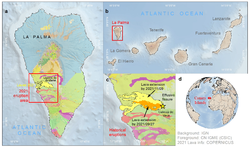
La Palma Island and Its 2021 Eruption
2. Materials: Geospatial Information
3. Methods
3.1. Inferring Lava Flow Rheology
3.2. Numerical Approach and Simulation of Lava Flow
3.3. CFL Adjustment Condition for Digital Terrain Model
3.4. Calibration Criteria
3.5. Simulations Set-Up
4. Results
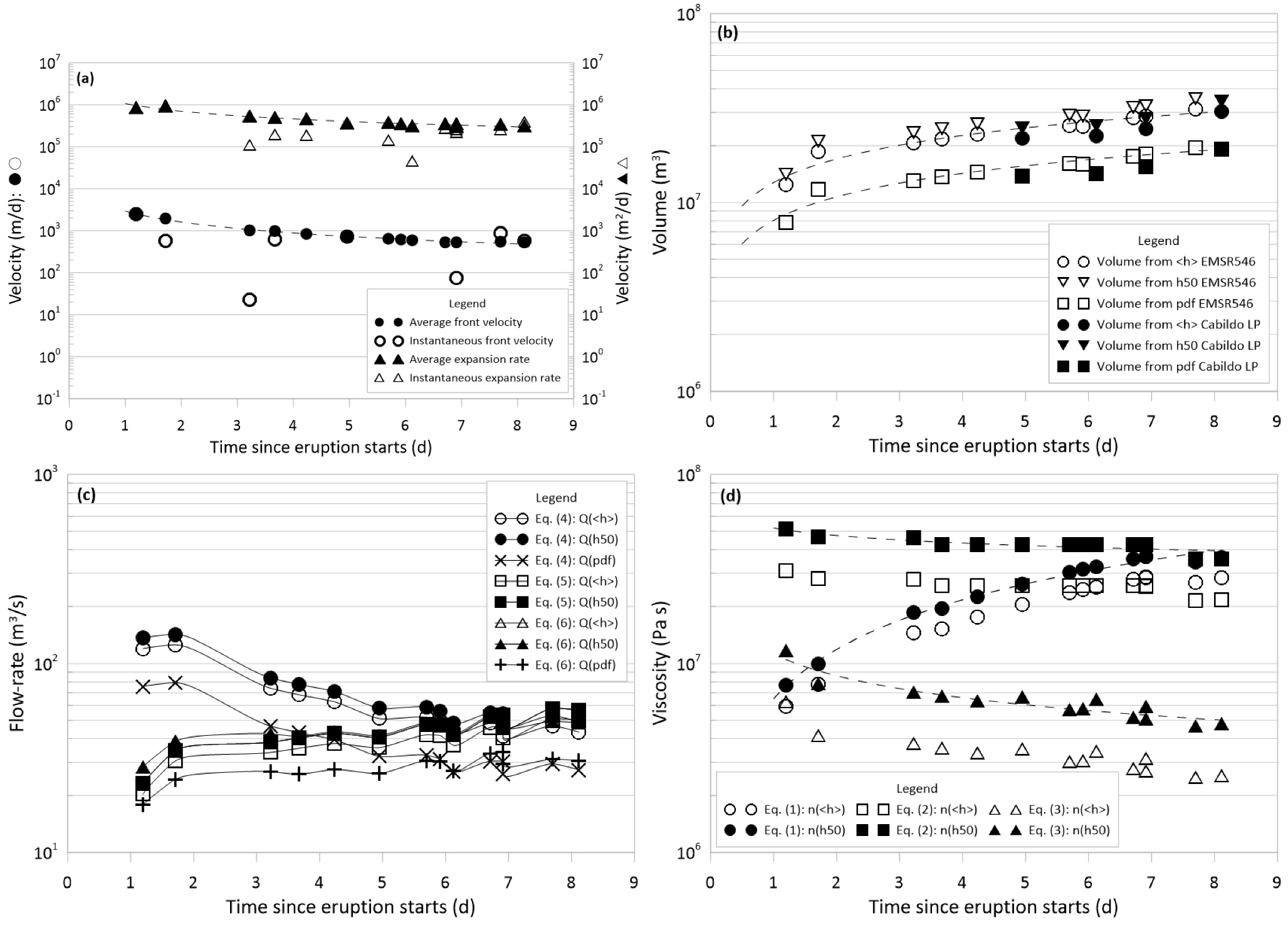
4.1. Flow Rate and Rheology Estimation from Morphometry
4.2. Numerical Simulation and Calibration Results
5. Discussion
6. Conclusions
Author Contributions
Funding
Acknowledgments
Conflicts of Interest
Abbreviations
| ASI | Agenzia Spaziale Italiana (Italy) |
| CFL | Courant–Friedrichs–Lewy |
| CNES | Centre national d’études spatiales (France) |
| CPU | Central Processing Unit or main processor |
| CSIC | Consejo Superior de Investigaciones Científicas (Spain) |
| DEM | Digital elevation model |
| DSM | Digital surface model |
| DTM | Digital terrain model |
| ESA | European Space Agency |
| GSD | Ground Sampling Distance |
| IGME | Instituto Geológico y Minero de España (Spain) |
| IGN | Instituto Geográfico Nacional (Spain) |
| INTA | Instituo Nacional Técnica Aeroespacial Esteban Terradas (Spain) |
| LiDAR | Laser Imaging Detection and Ranging |
| PEVOLCA | Plan de Emergencias Volcánicas de Canarias (Spain) |
| PNOA | Plan Nacional de Ortofotografía Aérea (Spain) |
| UAV | Unnamed Air Vehicle |
| UPM | Universidad Politécnica de Madrid (Spain) |
| UTM | Universal Transverse Mercator |
| MM | Marcos David Marquez (author) |
| CP | Carlos Paredes (author) |
| ML | Miguel Llorente (author) |
References
- Cardwell, R.; McDonald, G.; Wotherspoon, L.; Lindsay, J. Simulation of post volcanic eruption land use and economic recovery pathways over a period of 20 years in the Auckland region of New Zealand. J. Volcanol. Geotherm. Res. 2021, 415, 107253. [Google Scholar] [CrossRef]
- Deligne, N.I.; Jenkins, S.F.; Meredith, E.S.; Williams, G.T.; Leonard, G.S.; Stewart, C.; Wilson, T.M.; Biass, S.; Blake, D.M.; Blong, R.; et al. From anecdotes to quantification: Advances in characterizing volcanic eruption impacts on the built environment. Bull. Volcanol. 2022, 84, 7. [Google Scholar] [CrossRef]
- Del Negro, C.; Cappello, A.; Bilotta, G.; Ganci, G.; Hérault, A.; Zago, V. Living at the edge of an active volcano: Risk from lava flows on Mt. Etna. GSA Bull. 2020, 132, 1615–1625. [Google Scholar] [CrossRef]
- Tsang, S.W.R.; Lindsay, J.M.; Kennedy, B.; Deligne, N.I. Thermal impacts of basaltic lava flows to buried infrastructure: Workflow to determine the hazard. J Appl. Volcanol. 2020, 9, 8. [Google Scholar] [CrossRef]
- Wilson, G.; Wilson, T.M.; Deligne, N.I.; Cole, J.W. Volcanic hazard impacts to critical infrastructure: A review. J. Volcanol. Geotherm. Res. 2014, 286, 148–182. [Google Scholar] [CrossRef] [Green Version]
- Blong, R.J. Volcanic Hazards. A Sourcebook on the Effects of Eruptions. United States. 1984. Available online: https://www.osti.gov/biblio/7057586 (accessed on 22 November 2022).
- Blong, R.J. Volcanic hazards risk assessment. In Monitoring and Mitigation of Volcano Hazards; Scarpa, R., Tilling, R.I., Eds.; Springer: Berlin, Germany, 1996; pp. 675–698. [Google Scholar]
- Brown, S.K.; Jenkins, S.F.; Sparks, R.S.J.; Odbert, H.; Auker, M.R. Volcanic fatalities database: Analysis of volcanic threat with distance and victim classification. J. Appl. Volcanol. 2017, 6, 1–20. [Google Scholar] [CrossRef]
- Stewart, C.; Damby, D.E.; Horwell, C.J.; Elias, T.; Ilyinskaya, E.; Tomašek, I.; Longo, B.M.; Schmidt, A.; Carlsen, H.K.; Mason, E.; et al. Volcanic air pollution and human health: Recent advances and future directions. Bull. Volcanol. 2022, 84, 11. [Google Scholar] [CrossRef]
- Kilburn, C.R. Lava flow hazards and modeling. In The Encyclopedia of Volcanoes; Academic Press: London, UK, 2015; pp. 957–969. [Google Scholar] [CrossRef]
- Lekkas, E.; Meletlidis, S.; Kyriakopoulos, K.; Manousaki, M.; Mavroulis, S.; Kostaki, E.; Michailidis, A.; Gogou, M.; Mavrouli, M.; Castro-Melgar, I.; et al. The 2021 Cumbre Vieja volcano eruption in La Palma (Canary Islands). Newsl. Environ. Disaster Cris. Manag. Strateg. 2021, 26. [Google Scholar] [CrossRef]
- Barr, I.D.; Lynch, C.M.; Mullan, D.; De Siena, L.; Spagnolo, M. Volcanic impacts on modern glaciers: A global synthesis. Earth-Sci. Rev. 2018, 182, 186–203. [Google Scholar] [CrossRef]
- Delgado Granados, H.; Julio Miranda, P.; Carrasco Núñez, G.; Pulgarín Alzate, B.; Mothes, P.; Moreno Roa, H.; Cáceres Correa, B.E.; Cortés Ramos, J. Chapter 17—Hazards at ice-clad volcanoes: Phenomena, processes and examples from Mexico, Colombia, Ecuador and Chile. In Hazards and Disasters Series Snow and Ice-Related Hazards, Risks and Disasters, 2nd ed.; Haeberli, W., Whiteman, C., Eds.; Elsevier: Amsterdam, The Netherlands, 2021; pp. 597–639. ISBN 9780128171295. [Google Scholar]
- Major, J.J.; Newhall, C.G. Snow and ice perturbation during historical volcanic eruptions and the formation of lahars and floods. Bull. Volcanol. 1989, 52, 1–27. [Google Scholar] [CrossRef]
- Waythomas, C.F. Water, ice and mud: Lahars and lahar hazards at ice- and snow-clad volcanoes. Geol. Today 2014, 30, 34–39. [Google Scholar] [CrossRef]
- Mason, E.; Wieser, P.E.; Liu, E.J.; Edmonds, M.; Ilyinskaya, E.; Whitty, R.C.W.; Mather, T.A.; Elias, T.; Nadeau, P.A.; Wilkes, T.C.; et al. Volatile metal emissions from volcanic degassing and lava-seawater interactions at Kīlauea Volcano, Hawai’i. Commun. Earth Environ. 2021, 2, 79. [Google Scholar] [CrossRef]
- Boreham, F.; Cashman, K.; Rust, A. Hazards from lava–river interactions during the 1783–1784 Laki fissure eruption. GSA Bull. 2020, 132, 2651–2668. [Google Scholar] [CrossRef]
- Kim, J.; Lin, S.-Y.; Oh, J. Quaternary lava tubes distribution in Jeju Island and their potential deformation risks. Nat. Hazards Earth Syst. Sci. Discuss. 2022. [Google Scholar] [CrossRef]
- Sauro, F.; Pozzobon, R.; Massironi, M.; De Berardinis, P.; Santagata, T.; De Waele, J. Lava tubes on Earth, Moon and Mars: A review on their size and morphology revealed by comparative planetology. Earth-Sci. Rev. 2020, 209, 103288. [Google Scholar] [CrossRef]
- Titos, M.; Martínez Montesinos, B.; Barsotti, S.; Sandri, L.; Folch, A.; Mingari, L.; Macedonio, G.; Costa, A. Long-term hazard assessment of explosive eruptions at Jan Mayen (Norway) and implications for air traffic in the North Atlantic. Nat. Hazards Earth Syst. Sci. 2022, 22, 139–163. [Google Scholar] [CrossRef]
- Harris, A.J.L.; Carn, S.; Dehn, J.; Del Negro, C.; Guđmundsson, M.T.; Cordonnier, B.; Barnie, T.; Chahi, E.; Calvari, S.; Catry, T.; et al. Conclusion: Recommendations and findings of the RED SEED working group. Detect. Model. Responding Effusive Erupt. Geol. Soc. 2016, 426, 567–648. [Google Scholar] [CrossRef]
- Latutrie, B.; Andredakis, I.; De Groeve, T.; Harris, A.J.L.; Langlois, E.; van Wyk de Vries, B.; Saubin, E.; Bilotta, G.; Cappello, A.; Crisci, G.M.; et al. Testing a geographical information system for damage and evacuation assessment during an effusive volcanic crisis. Detect. Model. Responding Effusive Erupt. Geol. Soc. 2016, 426, 649–672. [Google Scholar] [CrossRef]
- Chester, D. Volcanoes and Society; Edward Arnold: London, UK, 1993; xii + 356p. [Google Scholar]
- Cappello, A.; Vicari, A.; Del Negro, C. Retrospective validation of a lava-flow hazard map for Mount Etna volcano. Ann. Geophys. 2011, 54, 634–640. [Google Scholar] [CrossRef]
- Cappello, A.; Ganci, G.; Calvari, S.; Pérez, N.M.; Hernández, P.A.; Silva, S.V.; Cabral, J.; Del Negro, C. Lava flow hazard modeling during the 2014–2015 Fogo eruption, Cape Verde. J. Geophys. Res. Solid Earth 2016, 121, 2290–2303. [Google Scholar] [CrossRef] [Green Version]
- Crisci, G.M.; Rongo, R.; Di Gregorio, S.; Spataro, W. The simulation model SCIARA: The 1991 and 2001 lava flows at Mount Etna. J. Volcanol. Geotherm. Res. 2004, 132, 253–267. [Google Scholar] [CrossRef]
- Rowland, S.K.; Garbeil, H.; Harris, A.J.L. Lengths and hazards from channel-fed lava flows on Mauna Loa, Hawai’i, determined from thermal and downslope modeling with FLOWGO. Bull. Volcanol. 2005, 67, 634–647. [Google Scholar] [CrossRef]
- Chevrel, M.O.; Favalli, M.; Villeneuve, N.; Harris, A.J.L.; Fornaciai, A.; Richter, N.; Derrien, A.; Boissier, P.; Di Muro, A.; Peltier, A. Lava flow hazard map of Piton de la Fournaise volcano. Nat. Hazards Earth Syst. Sci. 2021, 21, 2355–2377. [Google Scholar] [CrossRef]
- Crisci, G.M.; Di Gregorio, S.; Rongo, R.; Scarpelli, M.; Spataro, W.; Calvari, S. Revisiting the 1669 Etnean eruptive crisis using a cellular automata model and implications for volcanic hazard in the Catania area. J. Volcanol. Geotherm. Res. 2003, 123, 211–230. [Google Scholar] [CrossRef]
- Favalli, M.; Tarquini, S.; Fornaciai, A.; Boschi, E. A new approach to risk assessment of lava flow at Mt. Etna. Geology 2009, 37, 1111–1114. [Google Scholar] [CrossRef]
- Harris, A.J.L.; Favalli, M.; Wright, R.; Garbiel, H. Hazard assessment at Mount Etna using a hybrid lava flow inundation model and satellite-based land classification. Nat. Hazards 2011, 58, 1001–1027. [Google Scholar] [CrossRef]
- Kauahikaua, J.; Margriter, S.; Lockwood, J.; Trusdell, F. Applications of GIS to the estimation of lava flow hazards on Mauna Loa Volcano, Hawai’i. In Mauna Loa Revealed: Structure, Composition, History and Hazards; Rhodes, J.M., Lockwood, J.P., Eds.; American Geophysical Union, Geophysical Monographs: Washington, DC, USA, 1995; Volume 92, pp. 315–325. [Google Scholar]
- Kelfoun, K.; Vargas, S.V. VolcFlow capabilities and perspectives of development for the simulation of lava flows. In Detecting, Modelling and Responding to Effusive Eruptions; Special Publications; Harris, A.J.L., De Groeve, T., Garel, F., Carn, S.A., Eds.; Geological Society: London, UK, 2015; Volume 426. [Google Scholar] [CrossRef]
- Rongo, R.; Avolio, M.V.; Behncke, B.; D’Ambrosio, D.; Di Gregorio, S.; Lupiano, V.; Neri, M.; Spataro, W.; Crisci, G.M. Defining high-detail hazard maps by a cellular automata approach: Application to Mount Etna (Italy). Ann. Geophys. 2011, 54. [Google Scholar] [CrossRef]
- Marzocchi, W.; Newhall, C.; Woo, G. The scientific management of volcanic crises. J. Volcanol. Geotherm. Res. 2012, 247–248, 181–189. [Google Scholar] [CrossRef]
- Sheridan, M.; Malin, M. Application of computer-assisted mapping to volcanic hazard evaluation of surge eruptions: Vulcano, Lipari, and Vesuvius. J. Volcanol. Geotherm. Res. 1983, 17, 187–202. [Google Scholar] [CrossRef]
- Crisci, G.M.; Avolio, M.V.; Behncke, B.; D’Ambrosio, D.; Di Gregorio, S.; Lupiano, V.; Neri, M.; Rongo, R.; Spataro, W. Predicting the impact of lava flows at Mount Etna, Italy. J. Geophys. Res. 2010, 115, B04203. [Google Scholar] [CrossRef] [Green Version]
- Ishihara, K.; Iguchi, M.; Kamo, K. Numerical simulation of lava flows on some volcanoes in Japan. In Lava Flows and Domes. IAVCEI Proceedings in Volcanology, 2; Fink, D.J.H., Ed.; Springer: Berlin, Germany, 1990; pp. 174–207. [Google Scholar]
- Vicari, A.; Alexis, H.; Del Negro, C.; Coltelli, M.; Marsella, M.; Proietti, C. Modeling of the 2001 lava flow at Etna volcano by a Cellular Automata approach. Environ. Model. Softw. 2007, 22, 1465–1471. [Google Scholar] [CrossRef]
- Vicari, A.; Ganci, G.; Behncke, B.; Cappello, A.; Neri, M.; Del Negro, C. Near-real-time forecasting of lava flow hazards during the 12–13 January 2011 Etna eruption. Geophys. Res. Lett. 2011, 38. [Google Scholar] [CrossRef] [Green Version]
- Fujita, E.; Hidaka, M.; Goto, A.; Umino, S. Simulations of measures to control lava flows. Bull. Volcanol. 2009, 71, 401–408. [Google Scholar] [CrossRef]
- Scifoni, S.; Coltelli, M.; Marsella, M.; Proietti, C.; Napoleoni, Q.; Vicari, A.; Del Negro, C. Mitigation of lava flow invasion hazard through optimized barrier configuration aided by numerical simulation: The case of the 2001 Etna eruption. J. Volcanol. Geotherm. Res. 2010, 192, 16–26. [Google Scholar] [CrossRef]
- Chirico, G.D.; Favalli, M.; Papale, P.; Boschi, E.; Pareschi, M.T.; Mamou-Mani, A. Lava flow hazard at Nyiragongo volcano, D.R.C. 2. Hazard reduction in urban areas. Bull. Volcanol. 2009, 71, 375–387. [Google Scholar] [CrossRef]
- Becerril, L.; Bartolini, S.; Sobradelo, R.; Martí, J.; Morales, J.M.; Galindo, I. Long-term volcanic hazard assessment on El Hierro (Canary Islands). Nat. Hazards Earth Syst. Sci. 2014, 14, 1853–1870. [Google Scholar] [CrossRef] [Green Version]
- Becerril, L.; Martí, J.; Bartolini, S.; Geyer, A. Assessing qualitative long-term volcanic hazards at Lanzarote Island (Canary Islands). Nat. Hazards Earth Syst. Sci. 2017, 17, 1145–1157. [Google Scholar] [CrossRef] [Green Version]
- Felpeto, A.; Araña, V.; Ortiz, R.; Astiz, M.; García, A. Assessment and modelling of lava flow hazard on Lanzarote (Canary Islands). Nat. Hazards 2001, 23, 247–257. [Google Scholar] [CrossRef]
- Rodriguez-Gonzalez, A.; Aulinas, M.; Mossoux, S.; Perez-Torrado, F.J.; Fernandez-Turiel, J.L.; Cabrera, M.; Prieto-Torrell, C. Comparison of real and simulated lava flows in the Holocene volcanism of Gran Canaria (Canary Islands, Spain) with Q-LavHA: Contribution to volcanic hazard management. Nat. Hazards 2021, 107, 1785–1819. [Google Scholar] [CrossRef]
- Prieto-Torrell, C.; Rodriguez-Gonzalez, A.; Aulinas, M.; Fernandez-Turiel, J.L.; Cabrera, M.C.; Criado, C.; Perez-Torrado, F.J. Modelling and simulation of a lava Flow affecting a shore platform: A case study of Montaña de Aguarijo eruption, El Hierro (Canary Islands, Spain). J. Maps 2021, 17, 516–525. [Google Scholar] [CrossRef]
- Marrero, J.M.; García, A.; Berrocoso, M.; Llinares, A.; Rodríguez-Losada, A.; Ortiz, R. Strategies for the development of volcanic hazard maps in monogenetic volcanic fields: The example of La Palma (Canary Islands). J. Appl. Volcanol. 2019, 8, 6. [Google Scholar] [CrossRef] [Green Version]
- Martin-Naya, N. Análisis del Trazado de las Coladas de Lava a Través de Simulaciones en Cumbre Vieja, La Palma. Bachelor’s Thesis, Universidad de La Laguna, La Laguna, Spain, 2020; 70p. Available online: http://riull.ull.es/xmlui/handle/915/20842 (accessed on 22 November 2022). (In Spanish).
- Carracedo, J.C.; Troll, V.R.; Day, J.M.D.; Geiger, H.; Aulinas, M.; Soler, V.; Deegan, F.M.; Perez-Torrado, F.J.; Gisbert, G.; Gazel, E.; et al. The 2021 eruption of the Cumbre Vieja volcanic ridge on La Palma, Canary Islands. Geol. Today 2022, 38, 94–107. [Google Scholar] [CrossRef]
- Lev, E.; Birnbaum, J.; Hernandez, P.; Barrancos, J.; Tramontano, S.; Connor, L.; Connor, C.; Gabriel, J. Lava flow dynamics during the 2021 Cumbre Vieja eruption, La Palma, Spain. In Proceedings of the EGU General Assembly 2022, Vienna, Austria, 23–27 May 2022. EGU22-10531. [Google Scholar] [CrossRef]
- Román, A.; Tovar-Sánchez, A.; Roque-Atienza, D.; Huertas, I.E.; Caballero, I.; Fraile-Nuez, E.; Navarro, G. Unmanned aerial vehicles (UAVs) as a tool for hazard assessment: The 2021 eruption of Cumbre Vieja volcano, La Palma Island (Spain). Sci. Total Environ. 2022, 843, 157092. [Google Scholar] [CrossRef] [PubMed]
- Bernabeu, N.; Saramito, P.; Smutek, C. Modelling lava flow advance using a shallow-depth approximation for threedimensional cooling of viscoplastic flows. Geol. Soc. London, Spec. Publ. 2016, 426, 409–423. [Google Scholar] [CrossRef]
- Hunt, J.E.; Talling, P.J.; Clare, M.A.; Jarvis, I.; Wynn, R.B. Long-term (17 Ma) turbidite record of the timing and frequency of large flank collapses of the Canary Islands, Geochem. Geophys. Geosyst. 2014, 15, 3322–3345. [Google Scholar] [CrossRef] [Green Version]
- Romero, C. The Historical Volcanic Manifestations of the Canary Archipelago; Government of the Canary Islands (Department of Territorial Policy): Tenerife, Spain, 1991; Volume I, 695p. [Google Scholar]
- Carracedo, J.C.; Rodríguez Badiola, E.; Gouillou, H.; De La Nuez, J.; Pérez Torrado, F.J. Geology and volcanology of La Palma and El Hierro, Western Canaries. Estudios Geológicos 2001, 57, 175–273. [Google Scholar] [CrossRef] [Green Version]
- González-Alonso, E.; Lamolda, H.; Quirós, F.; Molina, A.J.; Fernández-García, A.; García-Cañada, L.; Pereda de Pablo, J.; Domínguez-Valbuena, J.; Prieto-Llanos, F.; Sáez-Gabarrón, L. Combination of geodetic techniques for deformation monitoring during 2021 La Palma eruption. In Proceedings of the EGU General Assembly 2022, Vienna, Austria, 23–27 May 2022. EGU22-10465. [Google Scholar] [CrossRef]
- Lopez, C.; Blanco, M.J.; Team, I. Instituto Geográfico Nacional Volcano Monitoring of the 2021 La Palma eruption (Canary Islands, Spain). In Proceedings of the EGU General Assembly 2022, Vienna, Austria, 23–27 May 2022. EGU22-11549. [Google Scholar] [CrossRef]
- Copernicus EMSR546, EMSN112, EMSN119, EMS INFORMATION BULLETIN Nr 151. Mobilisation and response of Copernicus Emergency Management Service for the Volcanic Eruption in La Palma (Spain). 2022. Available online: https://emergency.copernicus.eu/mapping/list-of-components/EMSR546/ (accessed on 22 November 2022).
- Farrell, J.A. Mapping the four-dimensional viscosity field of an experimental lava flow. J. Geophys. Res. Solid Earth 2020, 125, e2019JB018815. [Google Scholar] [CrossRef]
- Starodubtseva, Y.V.; Starodubtsev, I.S.; Ismail-Zadeh, A.T.; Tsepelev, I.A.; Melnik, O.E.; Korotkii, A.I. A method for magma viscosity assessment by lava dome morphology. J. Volcanol. Seismol. 2021, 15, 159–168. [Google Scholar] [CrossRef]
- Zeinalova, N.; Ismail-Zadeh, A.; Melnik, O.; Tsepelev, I.; Zobin, V. Lava Dome Morphology and Viscosity Inferred From Data-Driven Numerical Modeling of Dome Growth at Volcán de Colima, Mexico During 2007–2009. Front. Earth Sci. 2021, 9, 735914. [Google Scholar] [CrossRef]
- Lorite, S.; Ojeda, J.C.; Rodriguez-Cuenca, B.; González, C.; Muñoz, P. Procesado y distribución de nubes de puntos en el proyecto PNOA-LiDAR. Proceedingns of the XVII Congreso de la Asociación Española de Teledetección, Nuevas Plataformas y Sensores de Teledetección, Murcia, Spain, 3–7 October 2017. [Google Scholar]
- Castro, J.M.; Feisel, Y. Eruption of ultralow-viscosity basanite magma at Cumbre Vieja, La Palma, Canary Islands. Nat. Commun. 2022, 13, 3174. [Google Scholar] [CrossRef]
- Ganci, G.; Vicari, A.; Cappello, A.; Del Negro, C. An emergent strategy for volcano hazard assessment: From thermal satellite monitoring to lava flow modeling. Remote Sens. Environ. 2012, 119, 197–207. [Google Scholar] [CrossRef]
- Cordonnier, B.; Lev, E.; Garel, F. Benchmarking lava-flow models. Geol. Soc. Lond. Spec. Publ. 2016, 426, 425–445. [Google Scholar] [CrossRef]
- Dietterich, H.R.; Lev, E.; Chen, J.; Richardson, J.A.; Cashman, K.V. Benchmarking computational fluid dynamics models of lava flow simulation for hazard assessment, forecasting, and risk management. J. Appl. Volcanol. 2017, 6, 9. [Google Scholar] [CrossRef] [Green Version]
- Kavanagh, J.L.; Engwell, S.L.; Martin, S.A. A review of laboratory and numerical modelling in volcanology. Solid Earth 2018, 9, 531–571. [Google Scholar] [CrossRef] [Green Version]
- Cappello, A.; Hérault, A.; Bilotta, G.; Ganci, G.; Del Negro, C. MAGFLOW: A physics-based model for the dynamics of lava-flow emplacement. Geol. Soc. Lond. Spec. Publ. 2016, 426, 357–373. [Google Scholar] [CrossRef]
- Del Negro, C.; Fortuna, L.; Herault, A.; Vicari, A. Simulations of the 2004 lava flow at Etna volcano using the magflow cellular automata model. Bull. Volcanol. 2008, 70, 805–812. [Google Scholar] [CrossRef] [Green Version]
- Rongo, R.; Valeria, L.; Spataro, W.; D’Ambrosio, D.; Iovine, G.; Crisci, G. SCIARA: Cellular automata lava flow modelling and applications in hazard prediction and mitigation. Geol. Soc. Lond. Spec. Publ. 2015, 426. [Google Scholar] [CrossRef]
- Wadge, G.; Young, P.A.V.; McKendrick, I.J. Mapping lava flow hazards using computer simulation. J. Geophys. Res. Solid Earth 1994, 99, 489–504. [Google Scholar] [CrossRef]
- Young, P.; Wadge, G. FLOWFRONT: Simulation of a lava flow. Comput. Geosci. 1990, 16, 1171–1191. [Google Scholar] [CrossRef]
- Gallant, E.; Richardson, J.; Connor, C.; Wetmore, P.; Connor, L. A new approach to probabilistic lava flow hazard assessments, applied to the Idaho National Laboratory, eastern Snake River. Geology 2018, 46, 895–898. [Google Scholar] [CrossRef] [Green Version]
- Harris, A.; Rowland, S. FLOWGO: A kinematic thermorheological model for lava flowing in a channel. Bull. Volcanol. 2001, 63, 20–44. [Google Scholar] [CrossRef]
- Harris, A.J.L.; Rowland, S.K. FLOWGO 2012: An Updated Framework for Thermorheological Simulations of Channel-Contained Lava. In Hawaiian Volcanoes: From Source to Surface; Carey, R., Cayol, V., Poland, M., Weis, D., Eds.; John Wiley and Sons: Hoboken, NY, USA, 2015; pp. 457–482. [Google Scholar] [CrossRef]
- Proietti, C.; Coltelli, M.; Marsella, M.; Fujita, E. A quantitative approach for evaluating lava flow simulation reliability: LavaSIM code applied to the 2001 Etna eruption. Geochem. Geophys. Geosyst. 2009, 10, Q09003. [Google Scholar] [CrossRef]
- Tarquini, S.; Favalli, M. Mapping and DOWNFLOW simulation of recent lava flow fields at Mount Etna. J. Volcanol. Geotherm. Res. 2011, 204, 27–39. [Google Scholar] [CrossRef]
- Kelfoun, K.; Druitt, T.H. Numerical modelling of the emplacement of the 7500 BP Socompa rock avalanche. Chile J. Geophys. Res. 2005, 110, B12202. [Google Scholar] [CrossRef]
- Kelfoun, K.; Samaniego, P.; Palacios, P.; Barba, D. Testing the suitability of frictional behaviour for pyroclastic flow simulation by comparison with a well-constrained eruption at Tungurahua volcano (Ecuador). Bull. Volcanol. 2009, 71, 1057–1075. [Google Scholar] [CrossRef]
- De’ Michieli Vitturi, M.; Esposti Ongaro, T.; Lari, G.; Aravena, A. IMEX-SfloW2D 1.0: A depth-averaged numerical flow model for pyroclastic avalanches. Geosci. Model Dev. 2019, 12, 581–595. [Google Scholar] [CrossRef] [Green Version]
- Jasak, H.; Jemcov, A.; Tukovic, Z. OpenFOAM: A C++ library for complex physics simulations. In Proceedings of the International Workshop on Coupled Methods in Numerical Dynamics, Dubrovnik, Croatia, 19–21 September 2007; Terze, Z., Ed.; IUC: Dubrovnik, Croatia, 2007; pp. 1–20. [Google Scholar]
- Hérault, A.; Vicari, A.; Del Negro, C. A SPH thermal model for the cooling of a lava lake. In Proceedings of the 3rd International SPHERIC Workshop, Rome, Italy, 4–6 June 2008; pp. 4–6. [Google Scholar]
- Zago, V.; Bilotta, G.; Cappello, A.; Dalrymple, R.A.; Fortuna, L.; Ganci, G.; Hérault, A.; Del Negro, C. Preliminary validation of lava benchmark tests on the GPUSPH particle engine. Ann. Geophys. 2019, 62, VO224. [Google Scholar] [CrossRef]
- D’Ambrosio, D.; Filippone, G.; Rongo, R.; Spataro, W.; Trunfio, G.A. Cellular automata and GPGPU: An application to lava flow modeling. Int. J. Grid High Perform. Comput. 2012, 4, 30–47. [Google Scholar] [CrossRef] [Green Version]
- Saint-Venant, A.J.C. Théorie du mouvement non permanent des eaux, avec application aux crues des rivières et a l’introduction de marées dans leurs lits. Comptes Rendus Séances Acad. Sci. 1871, 73, 147–237. [Google Scholar]
- Walker, G.P.L. Lengths of lava flows. R. Soc. Lond. Philos. Transact. A 1973, 274, 107–118. [Google Scholar] [CrossRef]
- Lesher, C.E.; Spera, F.J. Thermodynamic and Transport Properties of Silicate Melts and Magma. In The Encyclopedia of Volcanoes, 2nd ed.; Elsevier Inc.: London, UK, 2015; pp. 113–141. [Google Scholar] [CrossRef]
- Harris, A.J.L.; Rowland, S.K. Effusion rate controls on lava flow length and the role of heat loss: A review. In Studies in Volcanology: The Legacy of George Walker; Special Publications of IAVCEI; Thordarson, T., Self, S., Larsen, G., Rowland, S.K., Hoskuldsson, A., Eds.; Geological Society: London, UK, 2009; Volume 2, pp. 33–51. [Google Scholar]
- Hon, K.; Gansecki, C.; Kauahikaua, J. The Transition from ‘A‘ā to Pāhoehoe crust on flows emplaced during the Pu‘u ‘Ō ‘ō -Kūpaianaha eruption. In The Pu‘u ‘Ō‘ō-Kūpaianaha Eruption of Kīlauea Volcano, Hawai‘i: The First 20 Years; U.S. Geological Survey Professional Paper 1676; Heliker, C., Swanson, D.A., Takahashi, T.J., Eds.; U.S. Geological Survey: Reston, VA, USA, 2003; pp. 89–103. [Google Scholar]
- Spera, F.J. Physical Properties of Magma. In Encyclopedia of Volcanoes; Sigurdsson, H., Ed.; Academic Press: San Diego, CA, USA, 2000; pp. 171–189. [Google Scholar]
- Hulme, G. The interpretation of lava flow morphology. Geophys. J. R. Astr. Soc. 1974, 39, 361–383. [Google Scholar] [CrossRef] [Green Version]
- McBirney, A.R.; Murase, T. Rheological properties of magmas. Annu. Rev. Earth Sci. 1984, 12, 337–357. [Google Scholar] [CrossRef]
- Shaw, H.R.; Wright, T.L.; Peck, D.L.; Okamura, R. The viscosity of basaltic magma: An analysis of field measurements in Makaopuhi lava lake, Hawaii. Am. J. Sci. 1968, 266, 255–265. [Google Scholar] [CrossRef]
- Pinkerton, H.; Sparks, R.S.J. Field measurements of the rheology of lava. Nature 1978, 276, 383–385. [Google Scholar] [CrossRef]
- Lev, E.; Spiegelman, M.; Wysocki, R.J.; Karson, J.A. Investigating Lava Flow Rheology Using Video Analysis and Numerical Flow Models. J. Volcanol. Geotherm. Res. 2012, 247–248, 62–73. [Google Scholar] [CrossRef] [Green Version]
- Robert, B.; Harris, A.; Gurioli, L.; Médard, E.; Sehlke, A.; Whittington, A. Textural and rheological evolution of basalt flowing down a lava channel. Bull. Volcanol. 2014, 76, 1–21. [Google Scholar] [CrossRef]
- Pinkerton, H.; Stevenson, R.J. Methods of determining the rheological properties of magmas at sub-liquidus temperatures. J. Volcanol. Geotherm. Res. 1992, 53, 47–66. [Google Scholar] [CrossRef]
- Roscoe, R. The viscosity of suspensions of rigid spheres. Br. J. Appl. Phys. 1952, 3, 267–269. [Google Scholar] [CrossRef]
- Griffiths, R.W. The dynamics of lava flows. Annu. Rev. Fluid Mech. 2000, 32, 477–518. [Google Scholar] [CrossRef]
- Belousov, A.; Belousova, M. Dynamics and viscosity of ‘aa’ and pahoehoe lava flows of the 2012–2013 eruption of Tolbachik volcano, Kamchatka (Russia). Bull. Volcanol. 2018, 80, 1–23. [Google Scholar] [CrossRef] [Green Version]
- Chevrel, M.O.; Pinkerton, H.; Harris, A.J. Measuring the viscosity of lava in the field: A review. Earth-Sci. Rev. 2019, 196, 102852. [Google Scholar] [CrossRef]
- Chevrel, M.O.; Cimarelli, C.; deBiasi, L.; Hanson, J.B.; Lavallée, Y.; Arzilli, F.; Dingwell, D.B. Viscosity measurements of crystallizing andesite from Tungurahua volcano (Ecuador). Geochem. Geophys. Geosyst. 2015, 16, 870–889. [Google Scholar] [CrossRef] [Green Version]
- Ishibashi, H. Non-Newtonian behavior of plagioclase-bearing basaltic magma: Subliquidus viscosity measurement of the 1707 basalt of Fuji volcano, Japan. J. Volcanol. Geotherm. Res. 2009, 181, 78–88. [Google Scholar] [CrossRef]
- Kolzenburg, S.; Giordano, D.; Cimarelli, C.; Dingwell, D.B. In situ thermal characterization of cooling/crystallizing lavas during rheology measurements and implications for lava flow emplacement. Geochim. Cosmochim. Acta 2016, 195, 244–258. [Google Scholar] [CrossRef]
- Sehlke, A.; Whittington, A.; Robert, B.; Harris, A.; Gurioli, L.; Médard, E. Pahoehoe to ‘a‘a transition of Hawaiian lavas: An experimental study. Bull. Volcanol. 2014, 76, 1–20. [Google Scholar] [CrossRef]
- Vetere, F.; Sato, H.; Ishibashi, H.; De Rosa, R.; Donato, P. Viscosity changes during crystallization of a shoshonitic magma: New insights on lava flow emplacement. J. Mineral. Petrol. Sci. 2013, 108, 144–160. [Google Scholar] [CrossRef] [Green Version]
- Vona, A.; Romano, C.; Dingwell, D.B.; Giordano, D. The rheology of crystal-bearing basaltic magmas from Stromboli and Etna. Geochim. Cosmochim. Acta 2011, 75, 3214–3236. [Google Scholar] [CrossRef]
- Nichols, R.L. Viscosity of Lava. J. Geol. 1939, 47, 290–302. Available online: http://www.jstor.org/stable/30056598 (accessed on 22 November 2022). [CrossRef]
- Jeffreys, H. The flow of water in an inclined channel of rectangular section. Phil. Mag. 1925, 49, 793–807. [Google Scholar] [CrossRef]
- Warner, N.H.; Gregg, T.K.P. Evolved lavas on Mars? Observations from southwest Arsia Mons and Sabancaya volcano, Peru. J. Geophys. Res. 2003, 108. [Google Scholar] [CrossRef]
- Fink, J.H.; Griffiths, R.W. Radial spreading of viscous-gravity cur-rents with solidifying crust. J. Fluid Mech. 1990, 221, 485–500. [Google Scholar] [CrossRef]
- Guest, J.E.; Kilburn, C.R.J.; Pinkerton, H.; Duncan, A.M. The evolution of lava flow-fields: Observations of the 1981 and 1983 eruptions of Mount Etna, Sicily. Bull. Volcanol. 1987, 49, 527–540. [Google Scholar] [CrossRef]
- Harris, A.J.; Dehn, J.; Calvari, S. Lava effusion rate definition and measurement: A review. Bull. Volcanol. 2007, 70, 1–22. [Google Scholar] [CrossRef]
- Pinkerton, H.; Sparks, R.S.J. The 1975 sub-terminal lavas, mount etna: A case history of the formation of a compound lava field. J. Volcanol. Geotherm. Res. 1976, 1, 167–182. [Google Scholar] [CrossRef]
- Moore, H.J.; Schaber, G.G. An estimate of the yield strength of the Imbrium flows. In Proceedings of the 6th Lunar Science Conference, Houston, TX, USA, 17–21 March 1975; pp. 101–118. [Google Scholar]
- Kilburn, C.R.J.; Lopes, R.M.C. The growth of aa lava fields on Mount Etna, Sicily. J. Geophys. Res. 1988, 93, 14759–14772. [Google Scholar] [CrossRef]
- Crisp, J.; Stephen, B. Influence of crystallization and entrainment of cooler material on the emplacement of basaltic aa lava flows. J. Geophys. Res. Solid Earth 1994, 99, 11819–11831. [Google Scholar] [CrossRef]
- Cashman, K.; Carl, T.; James, K. Cooling and crystallization of lava in open channels, and the transition of Pāhoehoe Lava to ‘A‘ā. Bull. Volcanol. 1999, 61, 306–323. [Google Scholar] [CrossRef]
- Chevrel, M.O.; Platz, T.; Hauber, E.; Baratoux, D.; Lavallée, Y.; Dingwell, D.B. Lava flow rheology: A comparison of morphological and petrological methods. Earth Planet. Sci. Lett. 2013, 384, 109–120. [Google Scholar] [CrossRef] [Green Version]
- Davies, T.; McSaveney, M.; Kelfoun, K. Runout of the Soccompa volcanic debris avalanche, Chile: A mechanical explanation for low basal shear resistance. Bull. Volcanol. 2010, 72, 933–944. [Google Scholar] [CrossRef]
- Pouget, S.; Davies, T.; Kennedy, B.; Kelfoun, K.; Leyrit, H. Numerical modelling: A useful tool to simulate collapsing volcanoes. Geol. Today 2012, 28, 59–63. [Google Scholar] [CrossRef]
- Thouret, J.-C.; Arapa, E.; Charbonnier, S.; Guerrero, A.; Kelfoun, K.; Cordoba., G.; Rodriguez, D.; Santoni, O. Modeling Tephra Fall and Sediment-Water Flows to Assess Their Impacts on a Vulnerable Building Stock in the City of Arequipa, Peru. Front. Earth Sci. 2022, 10, 865989. [Google Scholar] [CrossRef]
- Kelfoun, K.; Druitt, T.H.; van Wyk de Vries, B.; Guilbaud, M.N. Topographic reflection of Socompa debris avalanche, Chile. Bull. Volcanol. 2008, 70, 1169–1187. [Google Scholar] [CrossRef]
- Kelfoun, K. Suitability of simple rheological laws for the numerical simulation of dense pyroclastic flows and long-runout volcanic avalanches. J. Geophys. Res. Solid Earth 2011, 116, b08209. [Google Scholar] [CrossRef]
- Kelfoun, K.; Giachetti, T.; Labazuy, P. Landslide-generated tsunamis at Réunion Island and their possible sedimentary record in Mauritius Island. In Proceedings of the EGU General Assembly, Vienne, France, 3–8 April 2011. EGU2011-2759. [Google Scholar] [CrossRef]
- Vallejo Vargas, S.X. Numerical Models of Volcanic Flows for an Estimation and Delimitation of Volcanic Hazards, the Case of Reventador Volcano (Ecuador). Doctoral Dissertation, Université Clermont Auvergne, Clermont-Ferrand, France, 2017; 317p. [Google Scholar]
- Harris, A.J.L. Lava flows. In Modeling Volcanic Processes: The Physics and Mathematics of Volcanism; Fagents, S.A., Gregg, T.K., Lopes, R.M., Eds.; Cambridge University Press: Cambridge, MA, USA, 2013; pp. 85–106. [Google Scholar]
- Iverson, R.M.; Denlinger, R.P. Flow of variably fluidized granular masses across three-dimensional terrain: 1. Coulomb mixture theory. J. Geophys. Res. 2001, 106, 537–552. [Google Scholar] [CrossRef]
- Courant, R.; Friedrichs, K.; Lewy, H. On the partial difference equations of mathematical physics. IBM J. Res. Dev. 1967, 11, 215–234. [Google Scholar] [CrossRef]
- Hirsch, C. Numerical Computation of Internal and External Flows: The Fundamentals of Computational Fluid Dynamics; Elsevier: Amsterdam, The Netherlands, 2007. [Google Scholar]
- Bilotta, G.; Cappello, A.; Hérault, A.; Del Negro, C. Influence of topographic data uncertainties and model resolution on the numerical simulation of lava flows. Environ. Model. Softw. 2019, 112, 1–15. [Google Scholar] [CrossRef]
- Mossoux, S.; Saey, M.; Bartolini, S.; Poppe, S.; Canters, F.; Kervyn, M. Q-LAVHA: A flexible GIS plugin to simulate lava flows. Comput. Geosci. 2016, 97, 98–109. [Google Scholar] [CrossRef]
- Tsang, S.W.R.; Lindsay, J.M.; Coco, G.; Deligne, N.I. The influence of surficial features in lava flow modelling. J. Appl. Volcanol. 2020, 9, 1–12. [Google Scholar] [CrossRef]
- Rumpf, M.E.; Lev, E.; Wysocki, R. The influence of topographic roughness on lava flow emplacement. Bull. Volcanol. 2018, 80, 1–17. [Google Scholar] [CrossRef]
- Aravena, A.; Bevilacqua, A.; Esposti Ongaro, T.; Neri, A.; Cioni, R. Calibration strategies of PDC kinetic energy models and their application to the construction of hazard maps. Bull. Volcanol. 2022, 84, 1–21. [Google Scholar] [CrossRef]
- Spataro, W.; D’Ambrosio, D.; Rongo, R.; Trunfio, G.A. An evolutionary approach for modelling lava flows through cellular automata. In Cellular Automata. ACRI 2004; Lecture Notes in Computer Science; Sloot, P.M.A., Chopard, B., Hoekstra, A.G., Eds.; Springer: Berlin/Heidelberg, Germany, 2004; Volume 3305, pp. 725–734. [Google Scholar] [CrossRef]
- Charbonnier, S.J.; Connor, C.B.; Connor, L.J.; Sheridan, M.F.; Oliva Hernández, J.P.; Richardson, J.A. Modeling the October 2005 lahars at Panabaj (Guatemala). Bull. Volcanol. 2018, 80, 4–16. [Google Scholar] [CrossRef]
- Neglia, F.; Sulpizio, R.; Dioguardi, F.; Capra, L.; Sarocchi, D. Shallow-water models for volcanic granular flows: A review of strengths and weaknesses of TITAN2D and FLO2D numerical codes. J. Volcanol. Geotherm. Res. 2021, 410, 107146. [Google Scholar] [CrossRef]
- Jaccard, P. Distribution de la flore alpine dans le bassin des Dranses et dans quelques régions voisines. Bull. Soc. Vaudoise Sci. Nat. 1901, 37, 241–272. [Google Scholar]
- Levandowsky, M.; Winter, D. Distance between Sets. Nature 1971, 234, 34–35. [Google Scholar] [CrossRef]
- Jaccard, P. Lois de distribution florale dans la zone alpine. Bull. Soc. Vaud. Sci. Nat. 1902, 38, 27–31. [Google Scholar]
- Kereszturi, G.; Cappello, A.; Ganci, G.; Procter, J.; Németh, K.; Del Negro, C.; Cronin, S.J. Numerical simulation of basaltic lava flows in the Auckland Volcanic Field, New Zealand—Implication for volcanic hazard assessment. Bull. Volcanol. 2014, 76, 1–17. [Google Scholar] [CrossRef]
- Richardson, P.; Karlstrom, L. The multi-scale influence of topography on lava flow morphology. Bull. Volcanol. 2019, 81, 21. [Google Scholar] [CrossRef]
- Tennant, E.; Jenkins, S.F.; Winson, A.; Widiwijayanti, C.; Gunawan, H.; Haerani, N.; Kartadinata, N.; Banggur, W.; Triastuti, H. Reconstructing eruptions at a data limited volcano: A case study at Gede (West Java). J. Volcanol. Geotherm. Res. 2021, 418, 107325. [Google Scholar] [CrossRef]
- Henley, M. Estudio Morfométrico de los Conos Volcánicos Monogénicos de Cumbre Vieja (La Palma, Islas Canarias). Master’s Thesis, Universidad Complutense de Madrid, Madrid, Spain, 2012; 44p. [Google Scholar]
- Cappello, A.; Bilotta, G.; Ganci, G. Modeling of Geophysical Flows through GPUFLOW. Appl. Sci. 2022, 12, 4395. [Google Scholar] [CrossRef]
- Costa, A.; Macedonio, G. Computational modeling of lava flows: A review. Spec.-Pap.-Geol. Soc. Am. 2005, 396, 209–218. [Google Scholar] [CrossRef]
- Harris, A.J.; Rhéty, M.; Gurioli, L.; Villeneuve, N.; Paris, R. Simulating the thermorheological evolution of channel-contained lava: FLOWGO and its implementation in EXCEL. In Detecting, Modelling and Responding to Effusive Eruptions; Harris, A.J.L., De Groeve, T., Garel, F., Carn, S.A., Eds.; Geological Society: London, UK, 2016; Volume 426. [Google Scholar] [CrossRef]
- Harris, A.J.L.; Flynn, L.P.; Keszthelyi, L.; Mouginis-Mark, P.J.; Rowland, S.K.; Resing, J.A. Calculation of lava effusion rates from Landsat TM data. Bull. Volcanol. 1998, 60, 52–71. [Google Scholar] [CrossRef]
- Wright, R.; Blake, S.; Harris, A.; Rothery, D. A simple explanation for the space-based calculation of lava eruption rates. Earth Planet. Sci. Lett. 2001, 192, 223–233. [Google Scholar] [CrossRef]
- Hyman, D.M.R.; Dietterich, H.R.; Patrick, M.R. Toward next-generation lava flow forecasting: Development of a fast, physics-based lava propagation model. J. Geophys. Res. Solid Earth 2022, 127, e2022JB024998. [Google Scholar] [CrossRef]
- Chevrel, M.O.; Harris, A.; Peltier, A.; Villeneuve, N.; Coppola, D.; Gouhier, M.; Drenne, S. Volcanic crisis management supported by near real-time lava flow hazard assessment at Piton de la Fournaise, La Réunion. Volcanica 2022, 5, 313–334. [Google Scholar] [CrossRef]
- Harris, A.; Chevrel, M.; Coppola, D.; Ramsey, M.; Hrysiewicz, A.; Thivet, S.; Villeneuve, N.; Favalli, M.; Peltier, A.; Kowalski, P.; et al. Validation of an integrated satellite-data-driven response to an effusive crisis: The April–May 2018 eruption of Piton de la Fournaise. Ann. Geophys. 2019, 61, 1–18. [Google Scholar] [CrossRef]


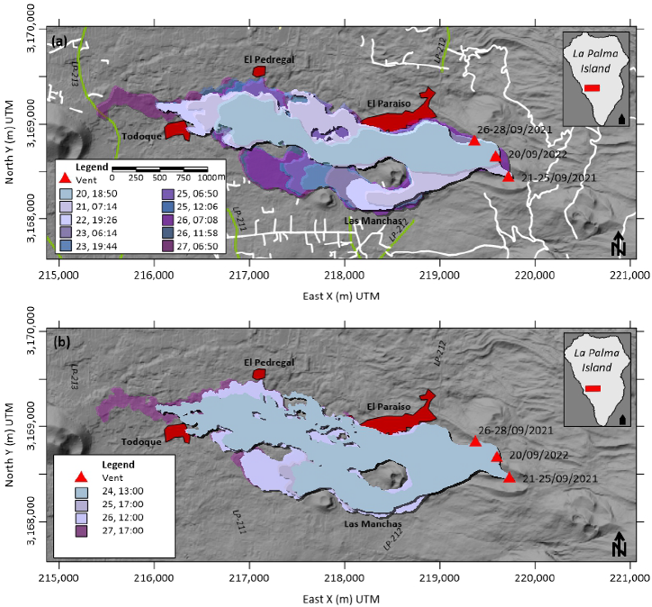
| Time UTC (dd/mm/yy-hh:mm) | Distribution Agency | Vehicle | Sensor | Expand Area (0.10 m) | Max. Length (m) |
|---|---|---|---|---|---|
| = 19/09/21-14:10 | Volcanic eruption starts | ||||
| = 20/09/21-18:50 | Copernicus | Cosmo-SM and Sentinel-1A/B | SAR | 102.8 1 | 3000 |
| = 21/09/21-07:14 | Copernicus | Cosmo-SM | SAR | 154.4 1 | 3297 |
| = 22/09/21-19:26 | Copernicus | Cosmo-SM | SAR | 171.1 1 | 3331 |
| = 23/09/21-06:14 | Copernicus | Cosmo-SM | SAR | 180.1 1 | 3614 |
| = 23/09/21-19:44 | Copernicus | Cosmo-SM | SAR | 190.7 1 | 3614 |
| = 24/09/21-13:00 | Cabildo La Palma | UAV | Optical | 181.7 2 | 3612 |
| = 25/09/21-06:50 | Copernicus | Cosmo-SM | SAR | 212.2 1 | 3614 |
| = 25/09/21-12:06 | Copernicus | Cosmo-SM and Pléiades | SAR Panchromatic | 210.2 1 | 3614 |
| = 25/09/21-17:00 | Cabildo La Palma | UAV | Optical | 187.1 2 | 3612 |
| = 26/09/21-07:08 | Copernicus | Cosmo-SM | SAR | 232.2 1 | 3614 |
| = 26/09/21-11:58 | Copernicus | Pléiades | Panchromatic | 237.5 1 | 3629 |
| = 26/09/21-12:00 | Cabildo La Palma | UAV | Optical | 231.9 2 | 3612 |
| = 27/09/21-06:50 | Copernicus | Cosmo-SM | SAR | 257.9 1 | 4312 |
| = 27/09/21-17:00 | Cabildo La Palma | UAV | Optical | 252.2 2 | 4296 |
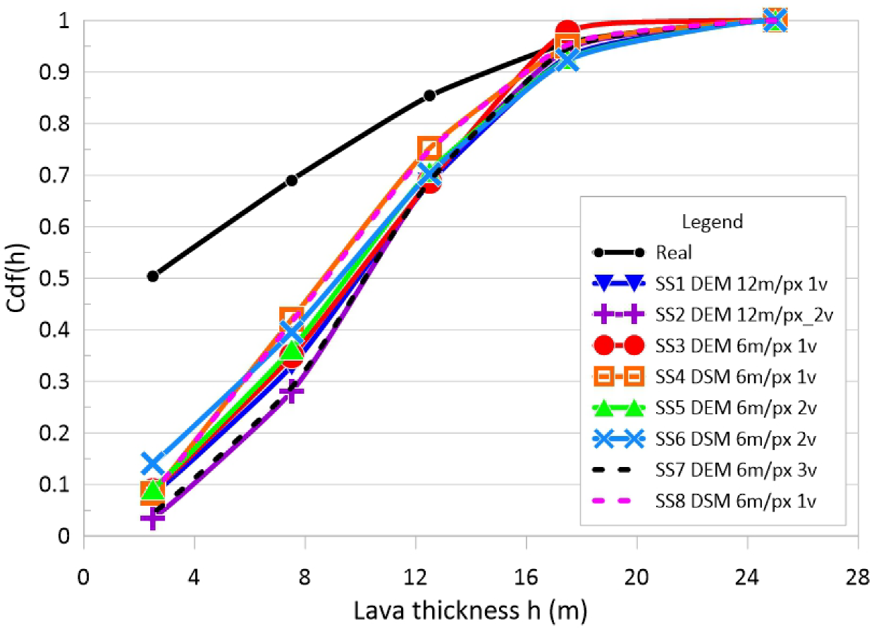
| Simulated Scenario | DTM | Resolution (m/px) | No. Vents | Coords (Long. Lat.) | Time Span (dd/mm–dd/mm) |
|---|---|---|---|---|---|
| SS1 | DEM | 12 | V1 | 5203 W 3653 N | 20–25 September |
| SS2 | DEM | 12 | V1 | 5203 W 3653 N | 20–21 September |
| V2 | 5157 W 3646 N | 21–25 September | |||
| SS3 | DEM | 6 | V1 | 5203 W 3653 N | 20–25 September |
| SS4 | DSM | 6 | V1 | 5203 W 3653 N | 20–25 September |
| SS5 | DEM | 6 | V1 | 5203 W 3653 N | 20–25 September |
| V2 | 5157 W 3646 N | 21–25 September | |||
| SS6 | DSM | 6 | V1 | 5203 W 3653 N | 20–25 September |
| V2 | 5157 W 3646 N | 21–25 September | |||
| SS7 | DEM | 6 | V1 | 5203 W 3653 N | 20–25 September |
| V2 | 5157 W 3646 N | 21–25 September | |||
| V3 (SW flank collapse) | 5210 W 3656 N | 25–27 September | |||
| SS8 | DSM | 6 | V1 | 5203 W 3653 N | 20–27 September |
| Simulated Scenario | Initial Estimated Flow Rate Q | Initial Estimated Viscosity | Best-Fit Flow Rate Q | Best-Fit Viscosity | Bes- Fit , , |
|---|---|---|---|---|---|
| SS1 | = 50 | 3 × 10 | = 65.21 | 2.9 × 10 | 5, 0, 36 × 10 |
| SS2 | = 131 | 7.6 × 10 | = 140.20 | 2.4 × 10 | 2.5, 0, 42 × 10 |
| = 50 | 3 × 10 | = 58.34 | 2.9 × 10 | 2.5, 0, 35 × 10 | |
| SS3 | = 50 | 3 × 10 | = 65.21 | 2.9 × 10 | 5, 0, 36 × 10 |
| SS4 | = 50 | 3 × 10 | = 65.21 | 2.9 × 10 | 5, 0, 36 × 10 |
| SS5 | = 131 | 7.6 × 10 | = 140.20 | 2.4 × 10 | 2.5, 0, 42 × 10 |
| = 50 | 3 × 10 | = 58.34 | 2.9 × 10 | 2.5, 0, 35 × 10 | |
| SS6 | = 131 | 7.6 × 10 | = 140.20 | 2.4 × 10 | 2.5, 0, 42 × 10 |
| = 50 | 3 × 10 | = 58.34 | 2.9 × 10 | 2.5, 0, 35 × 10 | |
| SS7 | = 131 | 7.6 × 10 | = 140.20 | 2.4 × 10 | 2.5, 0, 42 × 10 |
| = 50 | 3 × 10 | = 58.43 | 2.9 × 10 | 2.5, 0, 35 × 10 | |
| = 50 | 3 × 10 | = 57.25 | 2.9 × 10 | 2.5, 0, 35 × 10 | |
| SS8 | = 50 | 3 × 10 | = 63.63 | 2.9 × 10 | 5, 0, 36 × 10 |
Publisher’s Note: MDPI stays neutral with regard to jurisdictional claims in published maps and institutional affiliations. |
© 2022 by the authors. Licensee MDPI, Basel, Switzerland. This article is an open access article distributed under the terms and conditions of the Creative Commons Attribution (CC BY) license (https://creativecommons.org/licenses/by/4.0/).
Share and Cite
Marquez, M.; Paredes, C.; Llorente, M. Attempt to Model Lava Flow Faster Than Real Time: An Example of La Palma Using VolcFlow. GeoHazards 2022, 3, 529-562. https://doi.org/10.3390/geohazards3040027
Marquez M, Paredes C, Llorente M. Attempt to Model Lava Flow Faster Than Real Time: An Example of La Palma Using VolcFlow. GeoHazards. 2022; 3(4):529-562. https://doi.org/10.3390/geohazards3040027
Chicago/Turabian StyleMarquez, Marcos, Carlos Paredes, and Miguel Llorente. 2022. "Attempt to Model Lava Flow Faster Than Real Time: An Example of La Palma Using VolcFlow" GeoHazards 3, no. 4: 529-562. https://doi.org/10.3390/geohazards3040027