Comparing Root Cohesion Estimates from Three Models at a Shallow Landslide in the Oregon Coast Range

Abstract

Although accurate root cohesion model estimates are essential to quantify the effect of vegetation roots on shallow slope stability, few means exist to independently validate such model outputs. One validation approach for cohesion estimates is back-calculation of apparent root cohesion at a landslide site with well-documented failure conditions. The catchment named CB1, near Coos Bay, Oregon, USA, which experienced a shallow landslide in 1996, is a prime locality for cohesion model validation, as an abundance of data and observations from the site generated broad insights related to hillslope hydrology and slope stability. However, previously published root cohesion values at CB1 used the Wu and Waldron model (WWM), which assumes simultaneous root failure and therefore likely overestimates root cohesion. Reassessing published cohesion estimates from this site is warranted, as more recently developed models include the fiber bundle model (FBM), which simulates progressive failure with load redistribution, and the root bundle model-Weibull (RBMw), which accounts for differential strain loading. We applied the WWM, FBM, and RBMw at CB1 using post-failure root data from five vegetation species. At CB1, the FBM and RBMw predict values that are less than 30% of the WWM-estimated values. All three models show that root cohesion has substantial spatial heterogeneity. Most parts of the landslide scarp have little root cohesion, with areas of high cohesion concentrated near plant roots. These findings underscore the importance of using physically realistic models and considering lateral and vertical spatial heterogeneity of root cohesion in shallow landslide initiation and provide a necessary step towards independently assessing root cohesion model validity.

1. Introduction

Vegetation plays a critical role in protecting slopes against shallow landslides, primarily because of the mechanical reinforcement that plant roots provide to the soil on steep slopes [1,2,3,4]. In many upland areas, shallow landslide susceptibility increases in response to population and urbanization pressure, overgrazing, timber harvest [5], and climate-induced wildland fire size and frequency [6]. Over the last several decades, researchers have developed a variety of root breakage models to quantify the additional root cohesion provided to the soil [7,8]. These models vary significantly in their assumptions about the root reinforcement mechanics. For example, the earliest model developed by T.H. Wu, L.J. Waldron, and colleagues [9,10,11], known as the Wu and Waldron model (WWM), assumes that all roots break at once. This assumption was challenged by Pollen and Simon [12] in their fiber bundle model (FBM), a stress-controlled model that represents root breakage as a progressive process in which the weakest roots break and cause the load to be redistributed to the surviving roots. Instead of a stress-controlled model, Schwarz et al. [13] proposed a strain-controlled model called the root bundle model-Weibull (RBMw) that uses the Weibull distribution to represent the probability of breakage with increasing strain.

Since its publication, the WWM has been found to result in overestimation of root reinforcement in numerous studies due to its assumption of simultaneous failure [12,14]. By contrast, the FBM and the RBMw are generally considered to have more realistic assumptions [7]. However, despite the important role that root reinforcement plays in preventing shallow landslides, the authors are not aware of any studies that have compared results from these three models at a landslide site with the detailed measurements of root characteristics that are necessary for computing root cohesion with all three models. To the authors’ knowledge, only the study of Zydron and Skorski [15] has compared results from all three models together, but this study was conducted at an agricultural plot rather than at a landslide site. Similarly, while some studies have computed root cohesion using root data collected from shallow landslide sites [16,17], none of these studies compared more than two models. In this study, we use a unique dataset with detailed measurements of root characteristics, collected from the scarp of a shallow landslide, to calculate root cohesion using these three root breakage models. The comparison we present in this paper demonstrates how the choice of root breakage model affects root reinforcement estimates across an entire landslide site.

The study we present in this paper is important because the differences between the results of the three models at a landslide site could have significant implications for making engineering and land management decisions, such as the type, quantity, and extent of vegetation required to reinforce a slope [2,18]. Comparing these models at the same site would allow practitioners to adjust values that were previously estimated with one model to obtain values equivalent to estimation with another model. This type of comparison could be particularly valuable if other models are thought to be more realistic at that site. A better understanding of the magnitude and spatial variation of root reinforcement provided by different plant assemblages is necessary to evaluate potential negative impacts from different land use scenarios.

The previously instrumented research catchment in the Oregon Coast Range, CB1, is a thoroughly studied landslide site, with tightly constrained site characteristics, that is well suited for this type of comparative study. This catchment was heavily instrumented with hydrologic monitoring for several years before experiencing a landslide in 1996 [19]. Following the landslide, data from the catchment became the subject of several research studies on hillslope hydrology and slope stability [19,20,21,22,23,24]. As part of this research, Schmidt et al. [25] measured the tensile strength of vegetation roots at the site and used these data to estimate root reinforcement in the slope using the WWM. Since then, the development of the newer root breakage models, including the FBM and the RBMw, present the opportunity to revisit estimates of root cohesion at CB1.

This paper has two main objectives:

• To reexamine previously published root cohesion estimates for the CB1 landslide by Schmidt et al. [25], which was evaluated before the development of breakage models accounting for progressive root failure. Because root cohesion values for the CB1 slide have been cited and used in subsequent studies [19,21,22,26,27], reexamining these values has implications for these existing studies as well as future investigations.
• To compare the results of these three models at an instrumented landslide site where interpretations have implications for other shallow landslides. Because roots in the landslide scarp were surveyed and measured post-failure, data from the CB1 site is uniquely suited to this purpose.

In this study, we apply three different root breakage models to data from the CB1 catchment: (1) the WWM; (2) the global load-sharing FBM; and (3) the strain-controlled RBMw. These three models are representative of the major developments in root breakage models since the original publication of the WWM, as outlined by Dias et al. [7]. First, we review how root tensile strength was calculated based on laboratory analysis of root specimens collected at several locations in the Oregon Coast Range. We use these data to estimate regression models for predicting root tensile strength for roots of a given diameter and species. We then review the root data that were collected from the CB1 site after landsliding and use the regression models to calculate root tensile strengths. We then apply the three root breakage models to obtain estimates for apparent root cohesion. Finally, we investigate how root cohesion varies both laterally along the scarp perimeter and vertically with depth. We also investigate the contribution of each of five vegetation species to the overall root cohesion as a step towards independently validating cohesion estimates from different model frameworks.

2. Materials and Methods

2.1. Root Breakage Models

Plant roots reinforce a soil mass against shear failure because roots are strong in tension and weak in compression, whereas soil is weak in tension and strong in compression [28]. Root-reinforced soil is a composite material where roots of relatively high tensile strength reinforce a soil matrix of relatively low tensile strength [29]. The contribution of roots to the shear strength of soil can be described as an additional term in the widely adopted Mohr–Coulomb failure criterion:

$$s=c^{\prime }+c_r+\left(\sigma -u\right)\tan {\varphi }^{\prime },$$

(1)

where s is shear strength, σ is normal stress, u is pore-water pressure, ϕ’ is effective angle of soil internal friction, and c’ is the effective soil cohesion. The apparent root cohesion c_r represents the additional shear strength provided by roots [29]. Roots produce an apparent cohesion via fiber reinforcement, hereafter referred to as root cohesion. Most research quantifying root cohesion focuses on the tensile resistance of the root “bundle”. We focus on “breakage” models that calculate maximum tensile resistance of a root bundle where tensile strengths of the individual roots are known [7].

The WWM, the first quantitative model for estimating root bundle tensile strength, assumes that all roots fail simultaneously, mobilizing the sum of the full tensile strength of all roots. Several studies indicated that the WWM overestimates the strength because the assumption that all roots break simultaneously is not realistic; instead, roots break progressively, with the load from broken roots being redistributed onto surviving threads [12,14]. Pollen and Simon [12] therefore developed the fiber bundle model (FBM) to simulate progressive failure due to loading.

The greatest drawback of the FBM is that it does not account for root elasticity; the stress-step approach does not allow roots of different sizes to respond differently to the same applied load [15]. To address this shortcoming, Schwarz et al. [30] proposed a new model, the root bundle model (RBM), which uses a strain-step approach. Subsequently, Schwarz et al. [13] published an extension of the RBM, the root bundle model-Weibull (RBMw), which uses a Weibull probability distribution to account for variability in mechanical properties among roots of the same diameter.

Several studies have compared root cohesion estimates obtained between at least two of the published models. Preti and Schwarz [31] suggested multiplying the root cohesion by a correction factor to account for overestimation. Several studies have estimated this correction factor for the purpose of adjusting results obtained using the WWM [16,32,33]. One of the original authors of the WWM suggested reducing WWM estimates by a factor of 0.3–0.5 [34]. Arnone et al. [32] reports that the ratio of FBM-estimated cohesion to the WWM-estimated cohesion ranges from 0.34 to 1, with an average of 0.4 proposed by Preti and Schwarz [31]. Comparisons between the WWM and the RBMw suggest similar values for the ratio of WWM-estimated cohesion to RBMw-estimated cohesion, in the range of 0.4–0.6 [13,15], with Zydron and Skorski [15] proposing a correction factor of 0.5 for adjusting WWM-estimated cohesion.

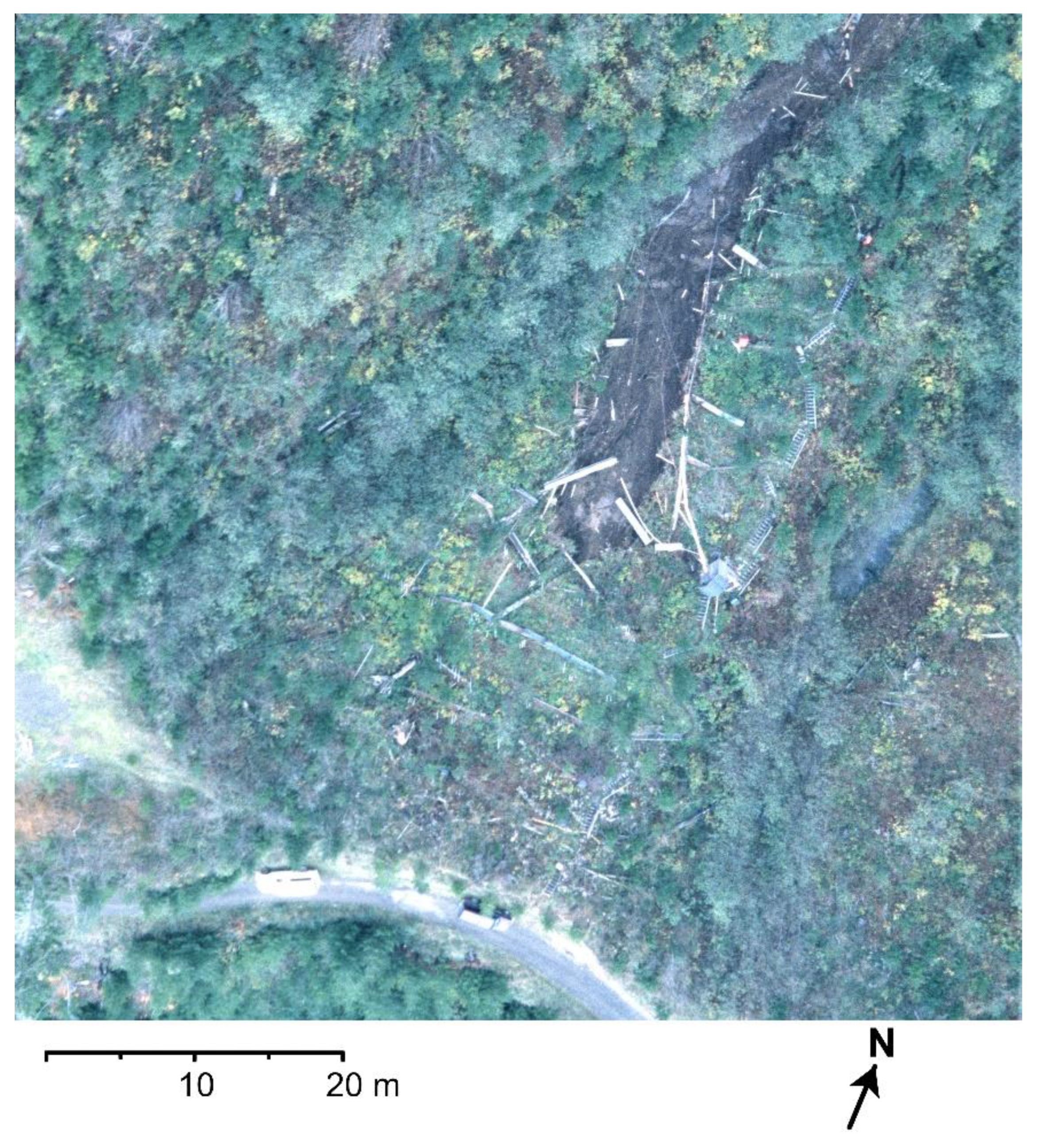
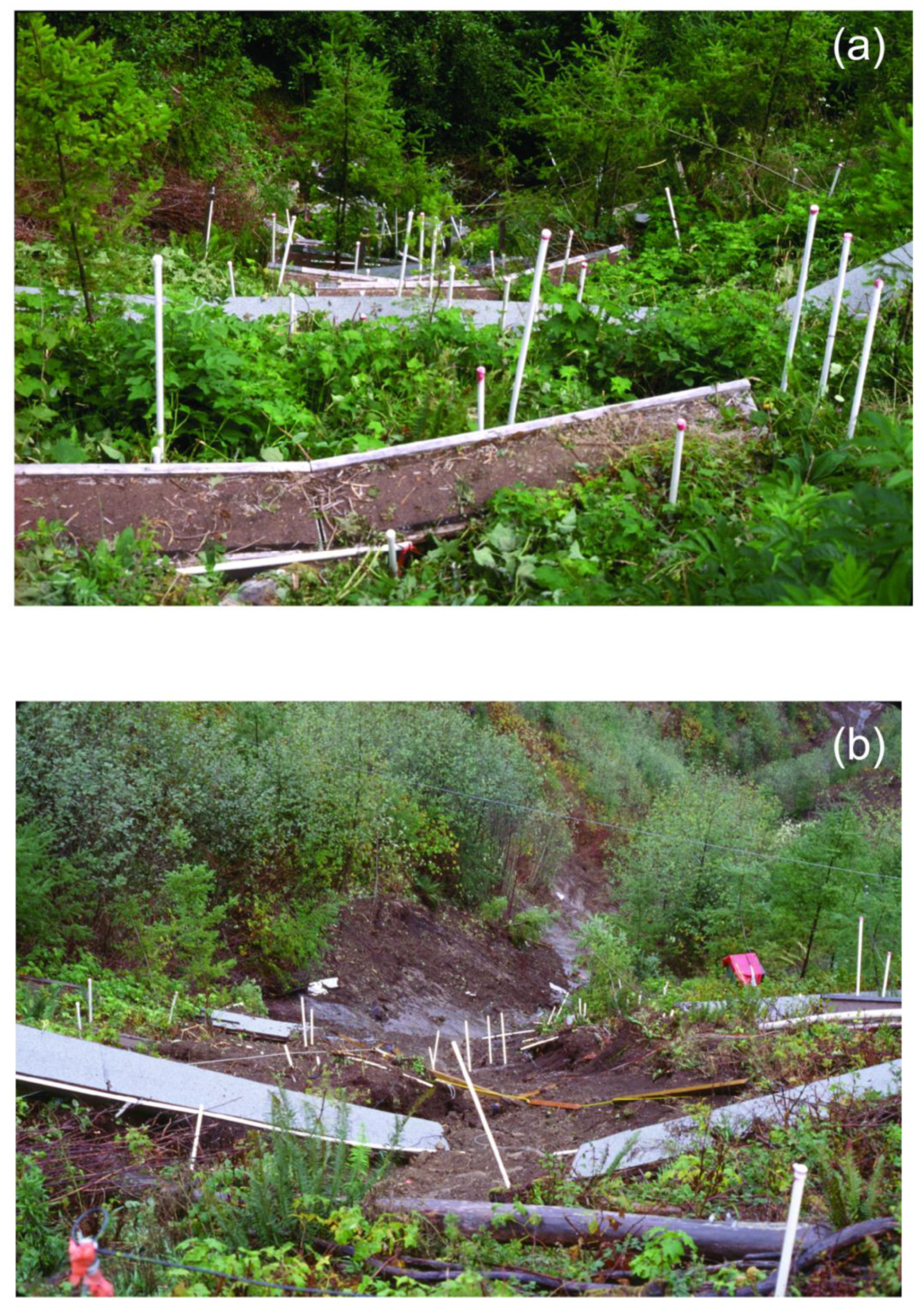
2.2. CB1 Landslide Site

The 860 m² CB1 catchment was monitored for unsaturated and saturated hydrologic flow response magnitude and pathways in the context of shallow-soil slope stability. CB1 is located below Mettman Ridge in the Oregon Coast Range, approximately 15 km northeast of Coos Bay, Oregon, USA [35]. The ridge crest elevation is approximately 300 m. A detailed physical description of the site and its soils is provided in Montgomery et al. [19] and Anderson et al. [20]. CB1 is one of two adjacent catchments used for experimental work on landslide failure [20,23,24]. The site was clearcut logged in 1987 and replanted with Douglas fir saplings in 1989; instrumentation was installed starting in 1989 and remained in place until November 1996, when it was destroyed by a landslide and the associated debris flow [19]. Figure 1 shows an aerial view of the CB1 catchment immediately after the landslide, and Figure 2 shows photos of the catchment both before and after the landslide taken from the same vantage point.

The CB1 site used artificial sprinkling experiments to understand hydrologic response [20,23,24]. Montgomery et al. [19] provides several photographs of the site before and after failure, as well as analysis of hydrologic conditions at the time of landslide initiation. The initial landslide source area was confined to the colluvium overlying sandstone bedrock with post-event observations constraining the failure mass upslope of the weir. The landslide and associated surface water flow stripped off most of the colluvium down to bedrock in the source area. After the landslide, the depth of the landslide scar from remnant ground surface to landslide failure surface was measured around the perimeter of the scar including lateral and head scarps components. The average depth of the landslide failure plane around the perimeter of the slide was 0.7 m but varied from 0.3 m to 1.2 m. The basal surface of the landslide scar was relatively planar, with an average slope of 43°, generally parallel to the ground surface. The basal area of the landslide scar was 157 m² and the total length of the upper scar was 58 m. However, roots from only 37 m of the scar perimeter could be collected and measured because of physical disturbance and obstruction by catwalk infrastructure [19].

After the 1996 failure, Schmidt et al. [25] meticulously measured and collected vegetation roots from the failure scarp. Vegetation in the vicinity of the failure scarp is dominated by Douglas fir (Pseudotsuga menziesii) saplings planted two years after the clear cut, blue elderberry (Sambucus caerulea), thimbleberry (Rubus parviflorus), foxglove (Digitalis purpurea), and Himalayan blackberry (Rubus discolor). All the plant species are native except for Himalayan blackberry, which is non-native and invasive [36]. Low confining stress triaxial tests on undisturbed material determined the colluvium was essentially cohesionless, with an internal friction angle of 40° [19]. Because very few roots intersected the basal landslide surface, and all the roots intersecting the lateral margin were observed to have broken, Schmidt et al. [25] concluded that plant roots mainly provided lateral reinforcement.

Previous root cohesion estimates at CB1, obtained using only the WWM [19,25], estimated a spatially averaged root cohesion of 4.6 kPa over the entire 37 m perimeter of the landslide scarp. These estimates were calculated in vertical and lateral profiles, revealing that root cohesion is spatially heterogeneous, with values ranging from near 0 to 13 kPa in the vertical profile dimension and near 0 to 14 kPa laterally along the scarp [19]. The basal component of root cohesion was estimated to be 0.1 kPa [19], a small fraction of the estimation for the roots exposed in the lateral scarp. The relatively low estimate for the basal component highlights the fact that most of the roots are constrained within the overlying colluvium, with few roots piercing the colluvium–bedrock interface.

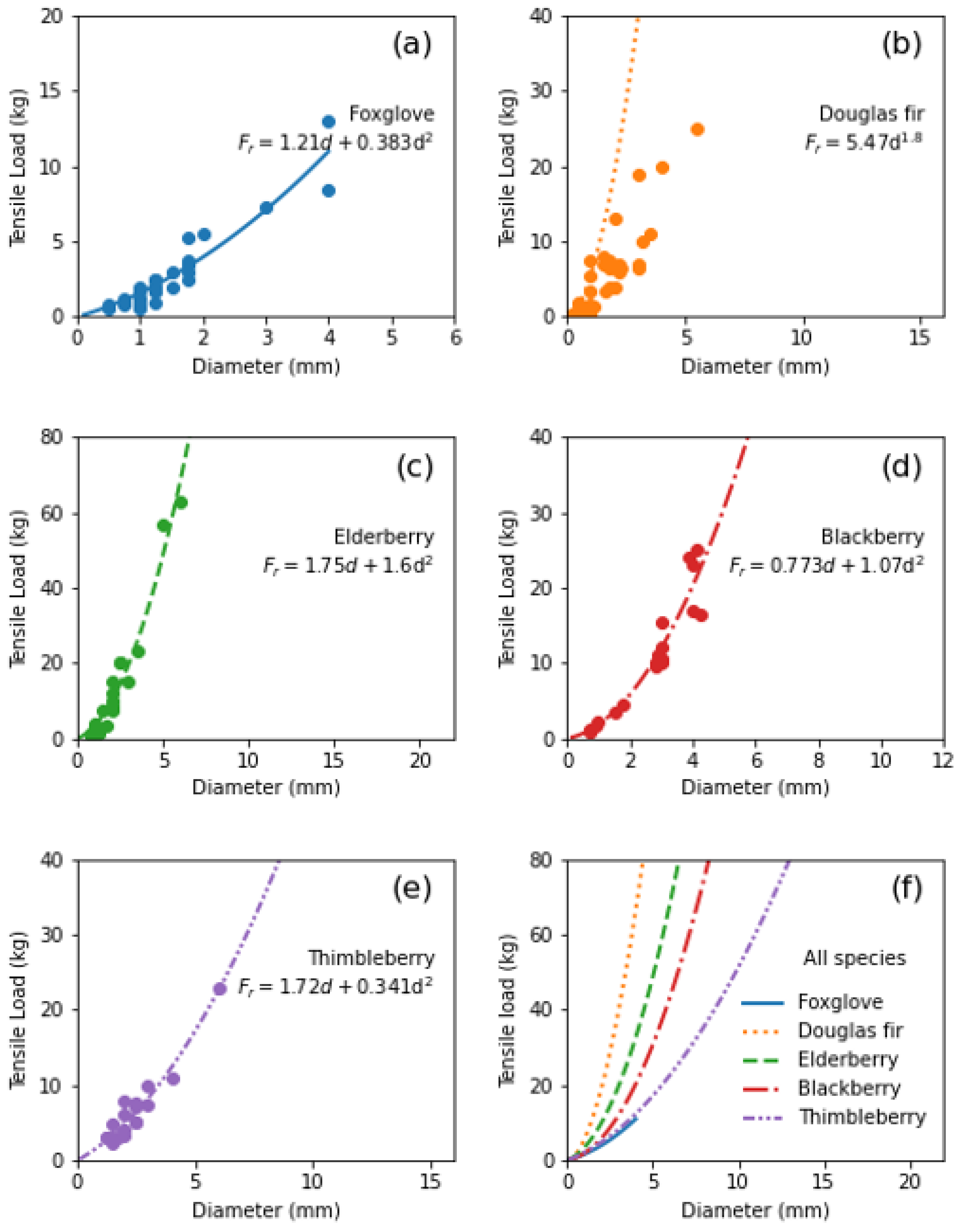
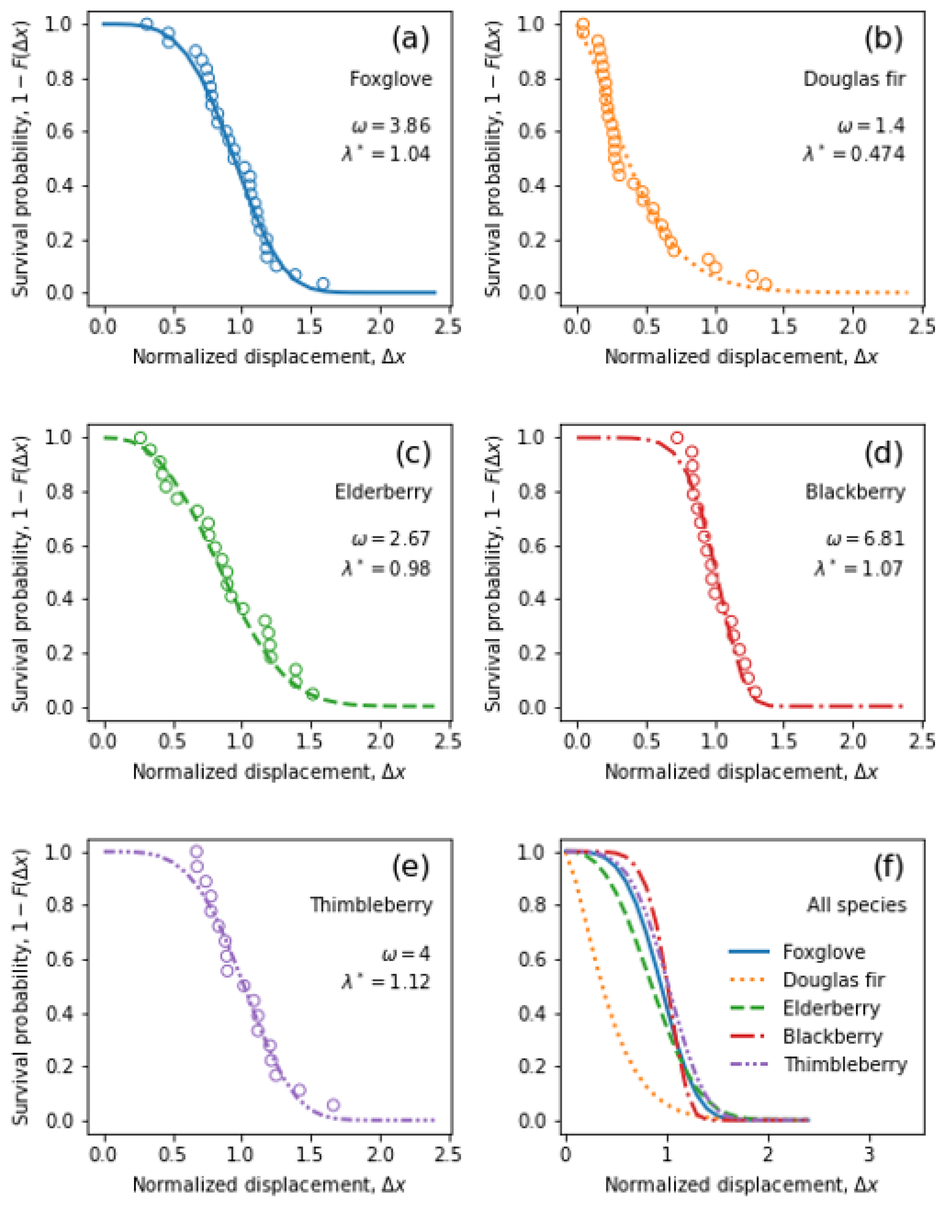
2.3. Estimation of Root Thread Strength from Experimental Data

Schmidt et al. [25] carried out tensile strength tests for root threads of 12 species at multiple sites throughout the Oregon Coast Range, including the Mettman Ridge area near Coos Bay. Schmidt et al. [25] collected root specimens measuring up to 6.5 mm in diameter by identifying healthy plant species in the field, excavating their roots, trimming suitable lengths of similar diameter, and determining the tensile force at failure for given diameter classes. Thread strength tests were conducted by adhering the ends of 15–20 cm-long threads into clamps, pulling by hand with a consistent force until the thread failed, and measuring the maximum force required for failure with calibrated springs. Healthy roots were identified based on bark characteristics and relatively high elasticity. We use the same method of estimating thread tensile strength as Schmidt et al. [25], who used a second-order polynomial regression model to represent maximum tensile load. To obtain results in units of tensile strength, which is necessary to apply the FBM, we convert the results of the polynomial regression model to a power law representing tensile strength (see Appendix A). We estimate maximum tensile load at failure for all species except Douglas fir. Because the Douglas fir roots measured were relatively fine and not representative of larger Douglas fir roots, we instead used the equation from Burroughs and Thomas [37] for the tensile load of Coast Douglas fir, which is based on a sample with greater representation of large-diameter roots. The experimental data and equations for tensile load are shown in Figure 3.

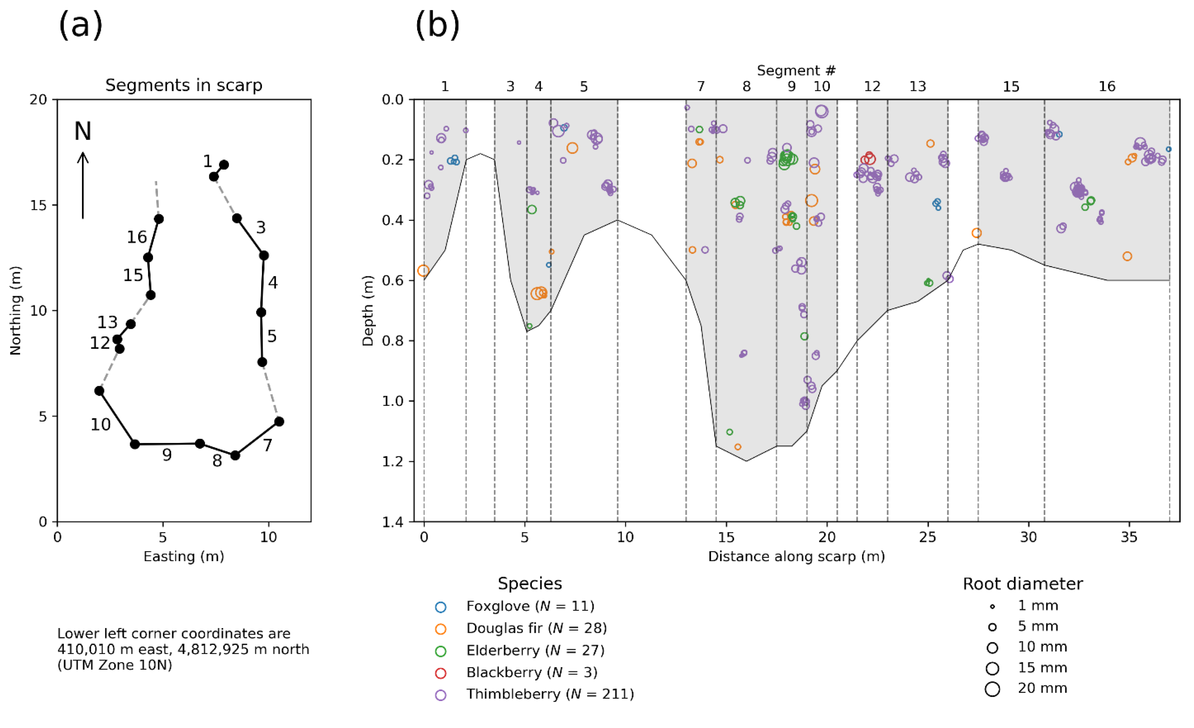
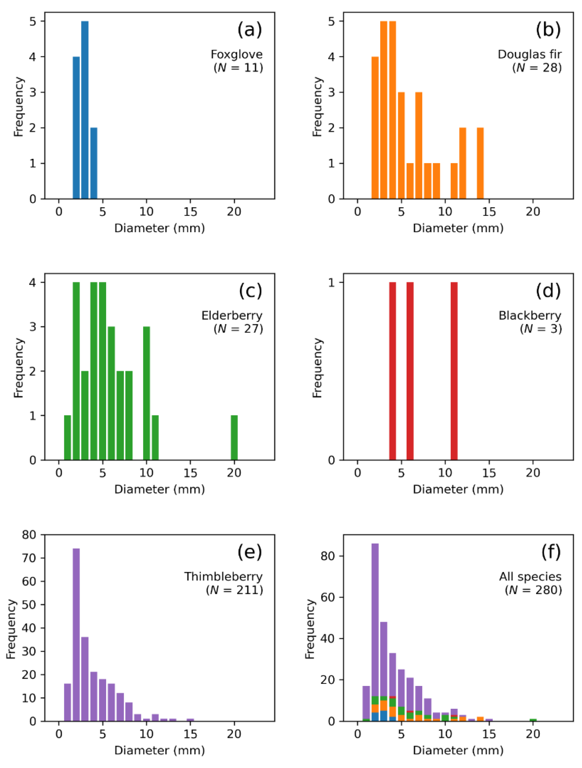
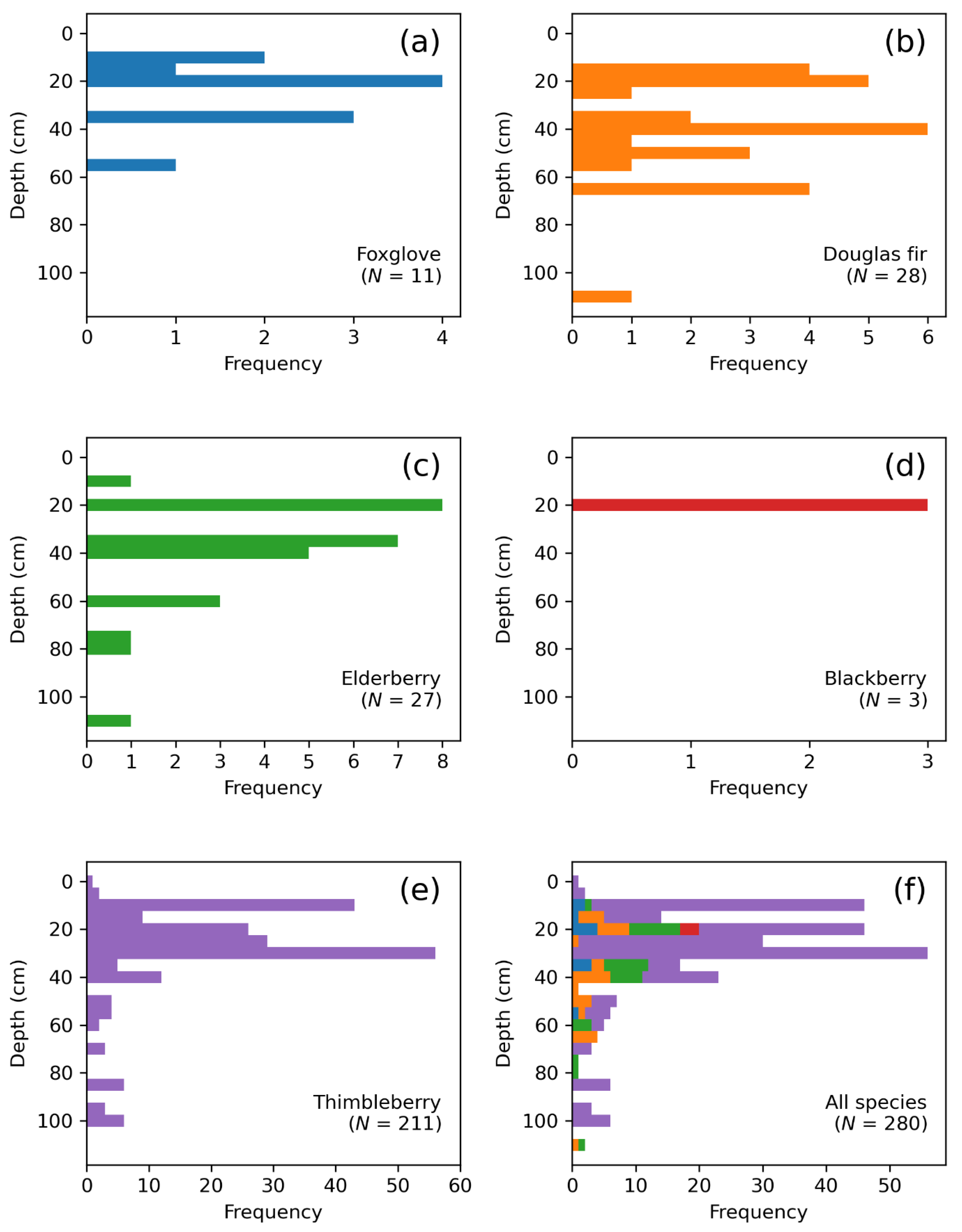
2.4. Root Data from the CB1 Landslide Site

Root data obtained from the CB1 landslide scarp are available in Schmidt and Cronkite-Ratcliff [35]. These data were collected by Schmidt et al. [25] and consist of 349 roots, 41 of which are located in the basal surface. All roots intersecting the slide scarp were broken during landsliding. These roots represent five different species: foxglove, Douglas fir, elderberry, blackberry, and thimbleberry. Of the remaining 308 roots that were not in the basal surface, 280 were live and generally oriented perpendicular to the failure surface and failed during landsliding. A subset of roots aligned roughly parallel to the slide scarp were exposed but did not fail during landsliding. The majority (211 out of 280; 75%) belonged to thimbleberry plants. It should be noted that the roots identified in the landslide headscarp were not excavated to the plant of origin to determine species. Rather, species were identified based on proximity to remaining above-ground plant biomass, and also by characteristic species traits (e.g., color, texture, tortuosity, bark, etc.) of the roots observed during the measurements of thread strength vs. diameter for the different species examined. The scarp was divided into 16 segments ranging from 1 to 6.2 m in width and from 0.29 to 1.2 m in average depth. However, roots were measured in only 12 of these 16 segments, with 4 segments occluded by ground disturbance (Figure 4). Segments are inclined at angles of 39–87° from horizontal. The area of each segment ranged from 0.5 to 4 m².

Figure 4 shows the location and diameter of the roots broken in the landslide scarp, and Figure 5 and Figure 6 show the diameter distribution and depth distribution for the roots broken in the landslide scarp. All the root species exhibit a roughly similar diameter distribution that is positive-skewed, with most values falling below 10 mm, and with modal values between 2 and 6 mm. The thickest observed root was an elderberry root with a diameter of 20 mm. The depth distributions for all species appear to be relatively similar, showing that most roots are located at relatively shallow depths. Approximately 90% of all roots are located within 50 cm of the ground surface. This is consistent with earlier research showing that in general, at least 80% of the biomass is within 40–50 cm of the ground surface [2].

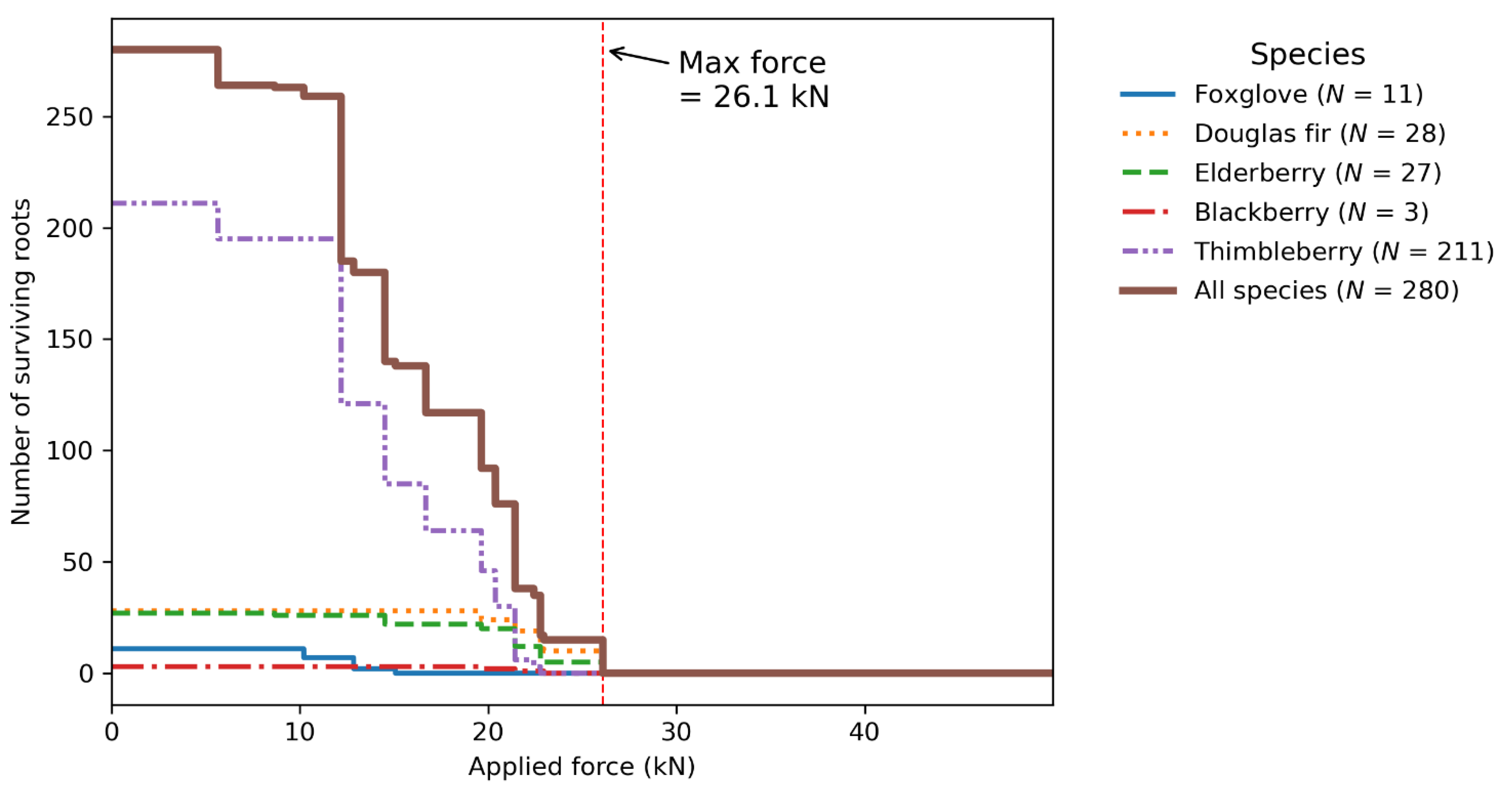
2.5. Application of Root Breakage Models

2.5.1. Wu and Waldron Model (WWM)

The WWM uses a simple calculation where the total force that can be sustained by the root bundle is the sum of the tensile strengths of all the individual roots in the bundle, multiplied by their cross-sectional areas.

$$F_b=R_f{{\displaystyle \sum }}_{i=1}^N{T}_i{A}_i,$$

(2)

where T_i is the tensile strength of the i-th root (in units of stress), A_i is area of the i-th root, and R_f is a correction factor for the inclination angle of the root. We use a value of 1.0 for R_f, following the conclusion of Thomas and Pollen-Bankhead [28] that an R_f value of 1.0 was most appropriate for sites with friction angles between 5° and 45° and failure surface angles between 10° and 90°.

2.5.2. Fiber Bundle Model (FBM)

Pollen and Simon [12] developed the FBM to address the systematic overestimation of root cohesion by the WWM, which assumes simultaneous failure of all roots. A single force is applied to a bundle of parallel fibers according to a load apportionment rule which determines the applied stress on each individual fiber. If the applied stress on a fiber exceeds its tensile strength, the fiber breaks, and it is no longer available to support the applied load in subsequent iterations. Effectively, this process finds the maximum total force that can be sustained by the entire bundle without breaking all the roots. Flowcharts describing the FBM are shown in Pollen and Simon [12] and Dias et al. [7].

In this study, we applied the FBM assuming global load sharing, in which the load is distributed equally among all fibers, rather than local load sharing, in which the load from a broken fiber is distributed disproportionally to its closer neighbors. In this study, we implement the FBM such that the load is distributed equally to each individual root, following the recommendation of Mao et al. [38]. This method of load apportionment ensures that the largest roots break last, making the total bundle strength dependent on the larger roots. This assumption is supported by Cohen et al. [39], who showed that small diameter roots will always be the first to break, and Giadrossich et al. [40], who showed that small roots provide almost no contribution to root reinforcement at the stand scale.

Note that any subset of roots with the same tensile strength and diameter will fail simultaneously. Therefore, in this study, where tensile strength is a function of diameter only, roots of the same species and diameter will either survive or fail together in a single model iteration.

Root Bundle Model-Weibull (RBMw)

The root bundle model-Weibull (RBMw) was developed to account for the effects of elastic deformation on root failure. Schwarz et al. [30] proposed a strain-controlled model, the RBM, that imposes successive displacements to a root bundle and calculates the resisting tensile force that results from the given strain. It is thus possible to calculate the forces acting on the root bundle for any displacement [41]. Schwarz et al. [13] further extended the RBM to account for variability in strength for roots of the same diameter. This extension was named the RBMw (root bundle model-Weibull) because they used a Weibull survival function to represent the decreasing probability of survival as the root is stretched beyond its original length.

The Weibull survival function represents the probability that a root remains unbroken when it has been stretched to a specific displacement. To model the elastic response of the root in a way that is independent of the root diameter, the displacement is normalized based on the elastic properties of the root. For details on how we implemented the RBMw, see Appendix B. The shape parameter ω and the scale parameter λ* of the Weibull survival function are estimated separately for each species. The resulting parameter values are shown in Figure 7.

2.6. Calculation of Root Cohesion

For each of the three models (WWM, FBM, and RBMw), the goal is to obtain the maximum force that can be sustained by the bundle. While the WWM directly gives an estimate of the maximum force, the FBM and RBMw produce a force value as a function of the nominal applied force or displacement, respectively. The FBM and RBMw therefore require application over a range of inputs to find the maximum force that can be sustained by the bundle. The root cohesion is calculated as the ratio of the maximum force F_b to the area of the failure surface (A):

$$c_r=F_b/A$$

(3)

The root cohesion can be calculated to give a scarp-averaged cohesion value for the entire bundle, without accounting for any spatial variability due to the spatial distribution of roots in the scarp. To obtain a spatially distributed estimate for root cohesion, the domain is discretized into sections (laterally and/or vertically), and the maximum force is calculated individually for each of these smaller sections ranging in cross-sectional area from 0.57 to 4.0 m² (when binned by segment) and from 0.42 to 3.3 m² (when binned by 10-cm depth intervals).

3. Results

First, we describe the results of the maximum force calculation across the entire landslide scarp without considering any spatial variability in the root cohesion. Figure 8 shows the number of surviving roots as a function of applied force from the FBM. Figure 9 shows the force-displacement curve from the RBMw. Whereas the WWM predicts a maximum force of 101.2 kN, the FBM predicts a much lower maximum force of 26.1 kN. The maximum force from the RBMw is lower still at 18.3 kN. These results are consistent with earlier research showing that the WWM overpredicts cohesion relative to the FBM and the RBMw [12,14]. Additionally, we draw the reader’s attention to the strain at which each species reaches its maximum activated force. Whereas both elderberry and Douglas fir exhibit peak values at about 200–300 mm of displacement, the maximum thimbleberry contribution to strength occurs at a much lower displacement value of about 40 mm.

In addition to the scarp-averaged values, we calculated the root cohesion distributed vertically and laterally within the scarp. Along with these distributed values, we describe the percent contribution to the overall bundle strength from vertical and lateral sections of the scarp. Because of the nonlinearity of the FBM and RBMw models, a general formula for the contribution of any one section k of the bundle is posed as a percent reduction in strength (PRS) for the bundle without group k:

$$PR{S}_k=100\left[\frac{\left(F_b-F_{\left(b-k\right)}\right)}{F_b}\right]$$

(4)

where F_b is the maximum force for the entire bundle, and F_(b−k) is the maximum force for the bundle with all the roots belonging to group k removed. Group k could represent a group of roots at a particular depth, a particular section along the perimeter of the scarp, and/or roots belonging to a specific species.

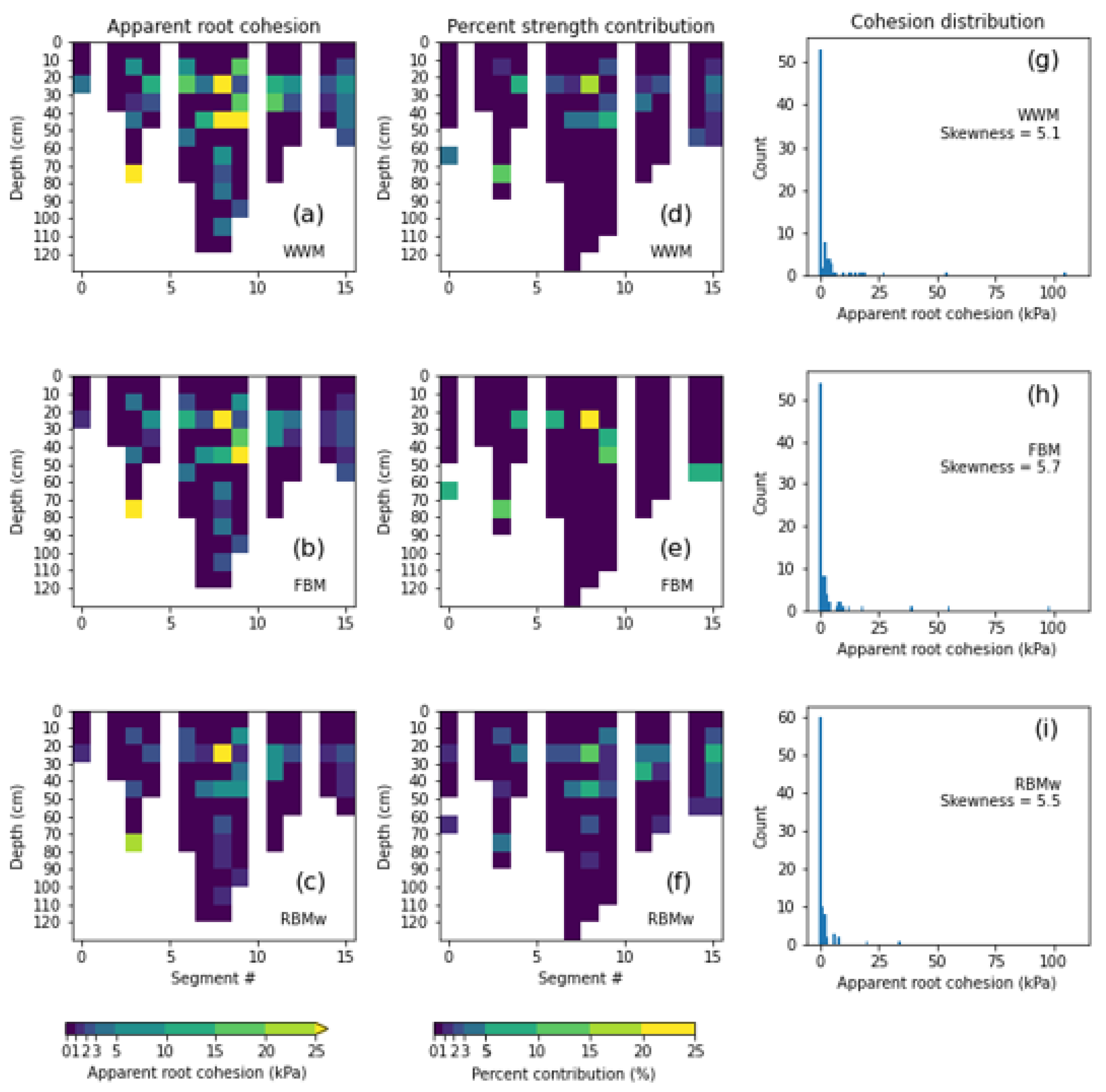
3.1. Scarp-Averaged Cohesion

When converted to root cohesion averaged over the entire 37 m long slide scarp, which has a total cross-sectional area of 21.8 m², the root cohesion is 4.6 kPa for the WWM, 1.2 kPa for the FBM, and 0.8 kPa for the RBMw. In their comparative study of the three models, Zydron and Skorski [15] obtained similar results for the relative cohesion estimates for two different tree species. However, the ratios of FBM-estimated cohesion and RBMw-estimated cohesion to the WWM-estimated cohesion, which are 0.18 and 0.26, respectively, are somewhat lower than estimates of comparable ratios from other researchers (see Section 2.1). Results for the scarp-averaged root cohesion are summarized in

Table 1. Results for root cohesion averaged over the entire CB1 landslide scarp.

Model	Maximum Force (kN)	Root Cohesion (kPa)	WWM Reduction Factor
WWM	101.2	4.6	1
FBM	26.1	1.2	0.26
RBMw	18.3	0.8	0.18

.

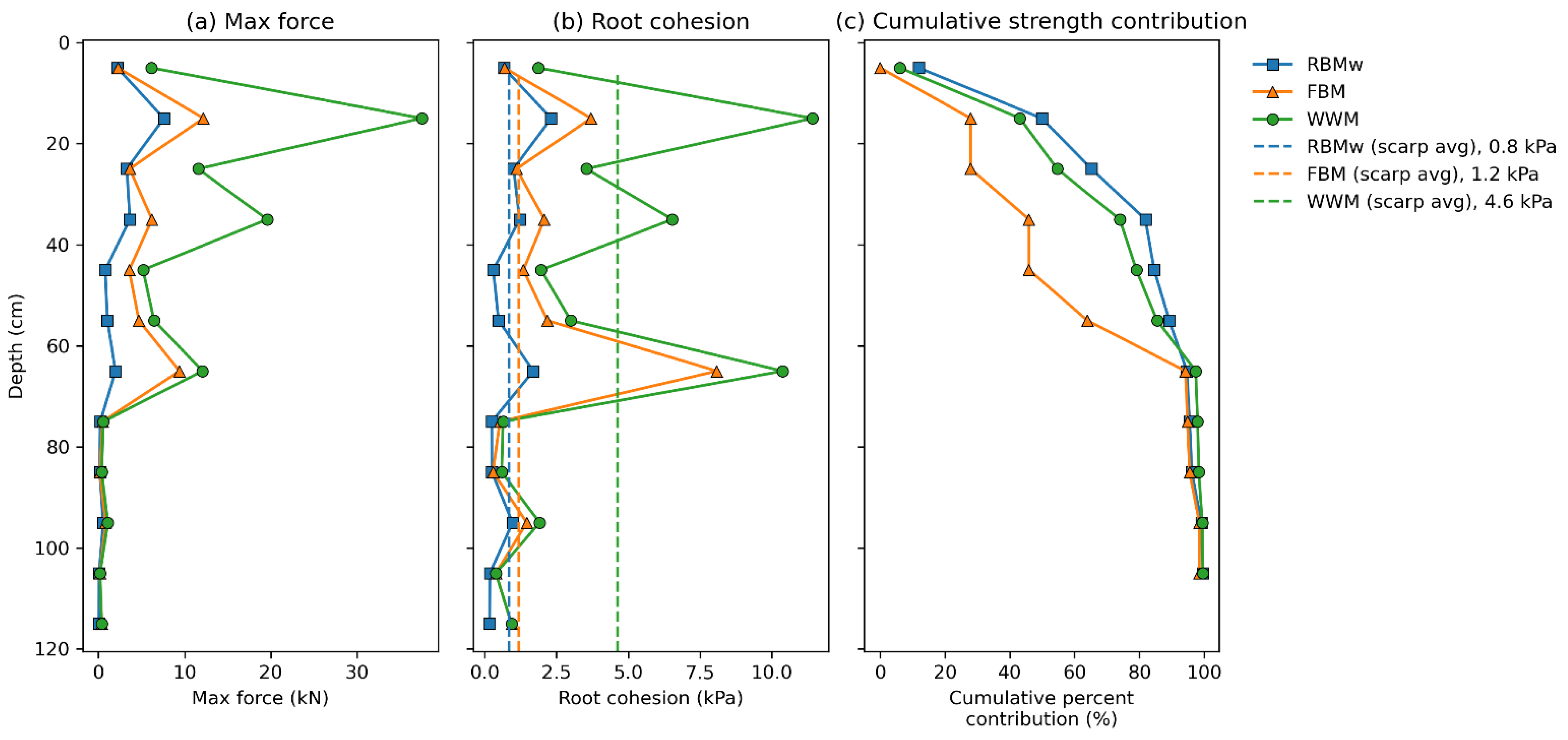
3.2. Root Cohesion by Depth

Root cohesion was calculated along different depth bins to highlight variability with depth below the ground surface. All three models show that cohesion diminishes below a depth of about 80 cm, with no model predicting cohesion greater than 2 kPa below this depth. However, there are substantial discrepancies in the cohesion values as well as the relationship versus depth that depend on the breakage model. The maximum root cohesion calculated by the WWM, for example, is 11.4 kPa, which is approximately 40% greater than the root cohesion calculated from the FBM at 8.1 kPa, and five times greater than the root cohesion calculated by the RBMw method at 2.3 kPa. The maximum activated forces and the root cohesion for the 10-cm depth bins are shown in Figure 10.

For the WWM and RBMw models, root cohesion reaches its maximum at a depth of 10–20 cm below the ground surface, and for these two models, roughly 80% of the root cohesion provided by these shallowly rooted plants species is in the top 40 cm of the regolith, with background negligible values at deeper soil depths. However, when using the FBM, the maximum cohesion occurs at a depth of approximately 60–70 cm below the ground surface. These results demonstrate the influence of the root strength model in calculating root cohesion and the implications for applying these values in the context of slope stability modeling in landscapes with plant species expressing different characteristic rooting depths. Similar results were reported by Zydron and Skorski [15], who reported that the WWM consistently produced the highest root cohesion values with depth, the RBMw produced the lowest, and the FBM produced values that fell between the results of the other two models.

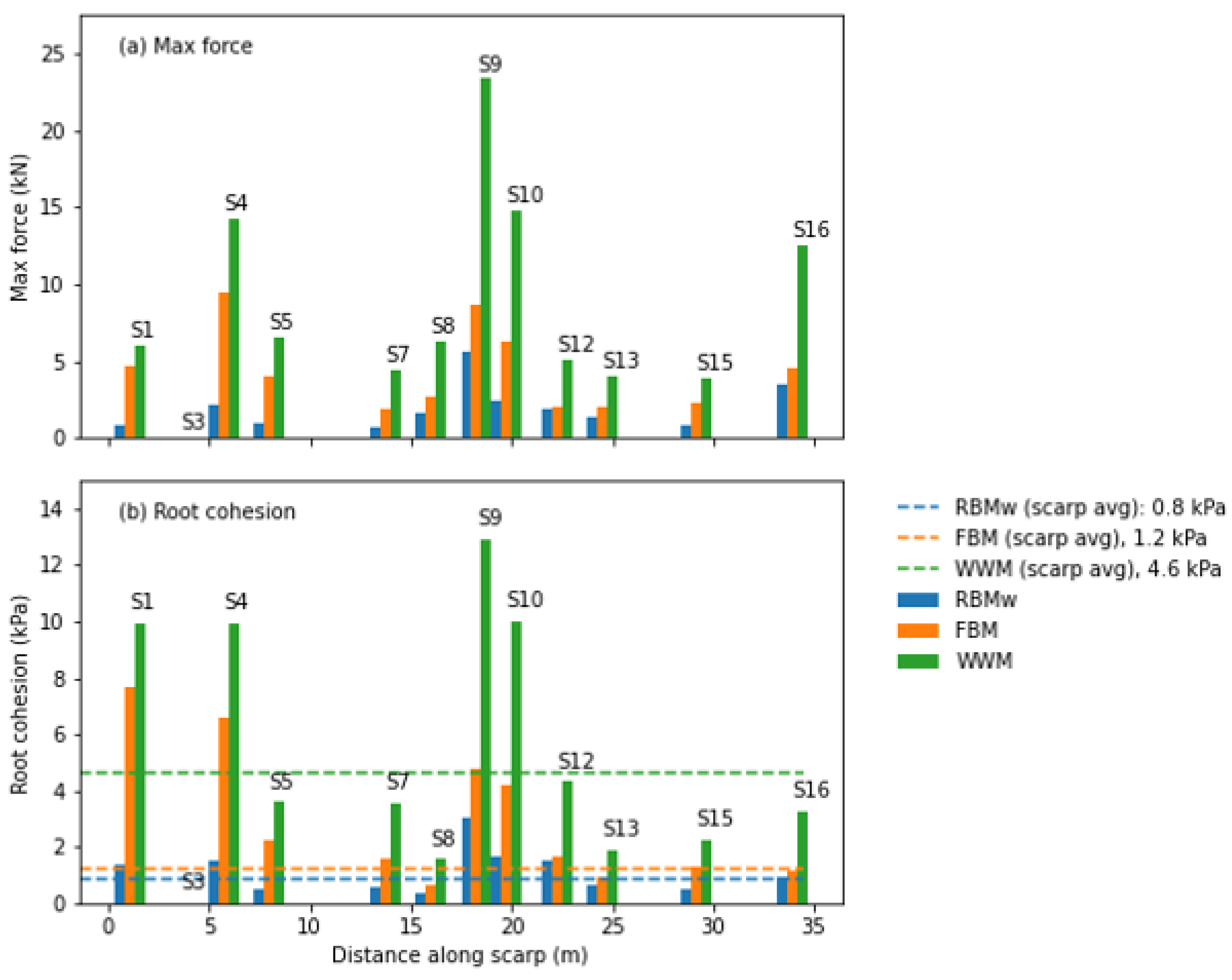
3.3. Root Cohesion along the Scarp Perimeter

The results also show that root cohesion is not homogeneous in the planform dimension along the perimeter of the landslide scarp. The maximum force and the cohesion calculated along the segments of the scarp are shown in Figure 11. For segment 3, the cohesion is <0.05 kPa for all three models, while in segment 9, the cohesion ranges from 3.1 kPa when calculated by the RBMw to 12.9 kPa when calculated by the WWM. The differences in the relative magnitudes of cohesion estimated by each of the three models are also evident in the depth-dependent and scarp-averaged cohesion values.

The planform distribution of root cohesion may be less informative than the depth distribution, since it mostly reflects the spatial location of roots belonging to specific plants, whereas the vertical distribution may be more indicative of a generalized relationship with depth. However, the lateral root distribution indicates areas of low root cohesion along the scarp perimeter, which could indicate gaps in vegetative root reinforcement and initiation areas for shallow landslides. For instance, Roering et al. [42] suggested that shallow landslides occur in areas of low root cohesion between trees; they presented a simple method for mapping of the distribution of trees and their canopies in hollows to quantify the landslide susceptibility.

Calculating the root cohesion by segment and by depth, as shown in Figure 12, provides more evidence that the cohesion has significant spatial heterogeneity. Although depth bins have a uniform size of 10 cm, the variation in the width of each segment results in the areas over which cohesion was calculated varying between 0.08 m² and 0.65 m². Figure 12 shows that cohesion is highly concentrated within areas that have a high density of elderberry and Douglas fir roots, which have the greatest tensile strengths. For all three models, the cohesion distribution among the different depth/segment sections has a skewness greater than 5, indicating the very high degree of spatial concentration. For the depth/segment sections with the greatest contribution, while most depth/segment sections contribute <1% to the overall root cohesion, the percent contribution for the strongest section is 16% for the WWM, 23% for the FBM, and 12% for the RBMw. Alternatively, the cohesion of the strongest individual section is 123 kPa for the WWM, 99 kPa for the FBM, and 34 kPa for the RBMw, values which are greater than the scarp-averaged cohesion calculated from the respective model by a factor greater than 25. This relation highlights the great spatial variability and localized maxima adjacent to denser, spatially concentrated, plant roots.

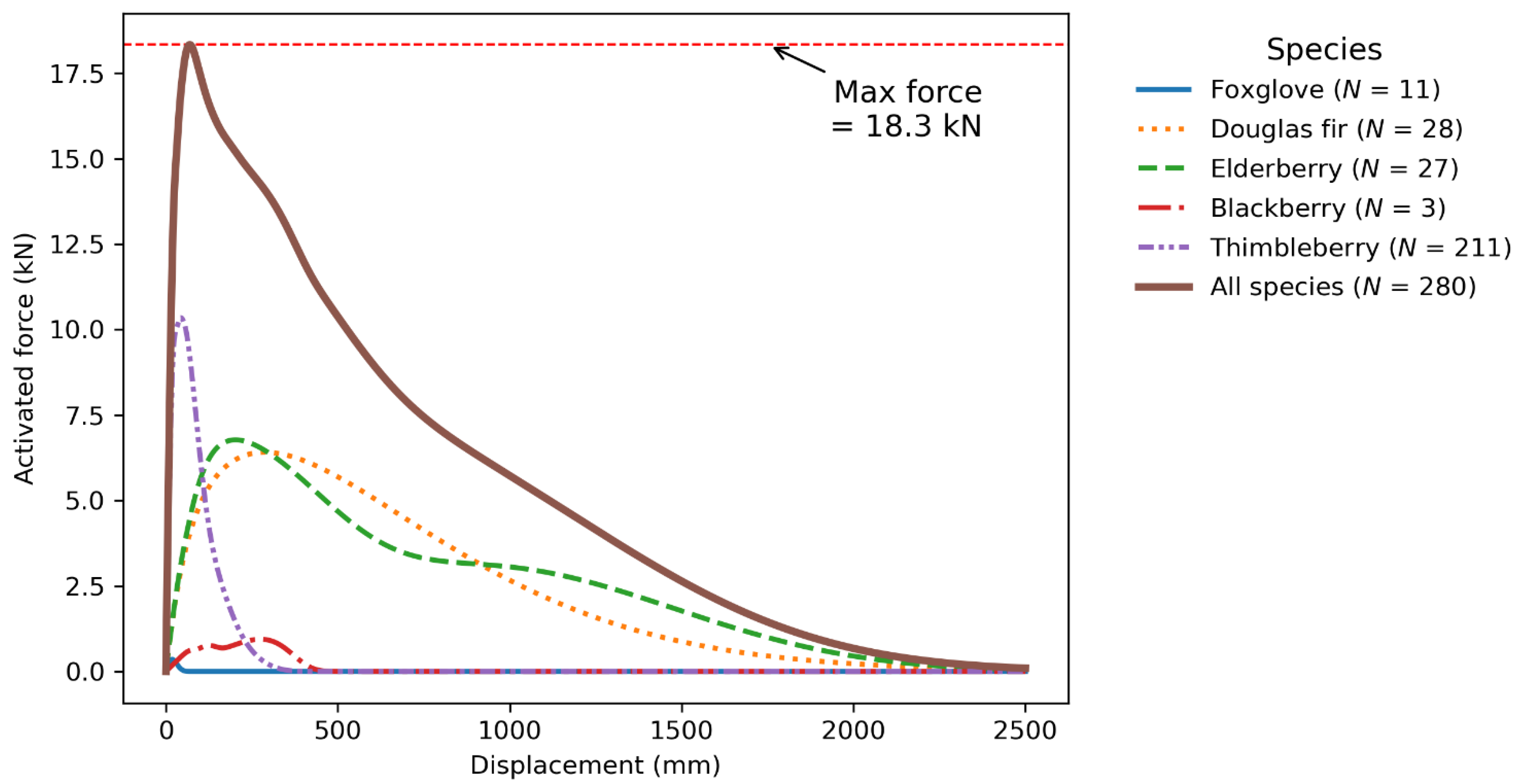
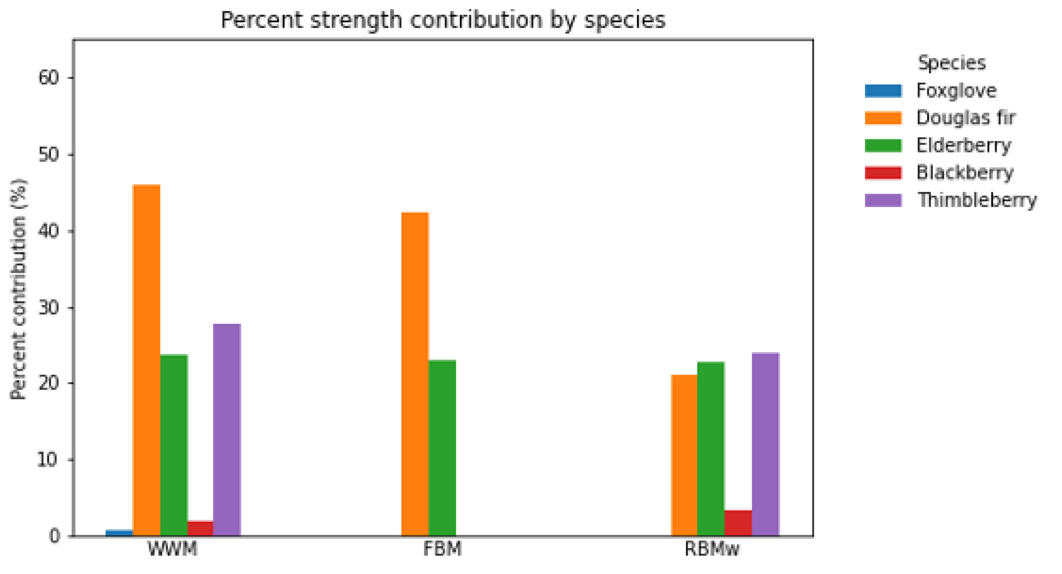
3.4. Contribution of Cohesion by Species

The amount of cohesion contributed by each of the species within the CB1 landslide scarp is an especially important question from a geotechnical engineering point of view because it addresses which species could be most effective for slope stabilization [2,18]. The contribution of root cohesion by a particular species represents the PRS that would occur if roots from that species were removed from the bundle, calculated using Equation (4). Figure 13 shows the contribution of root cohesion by species for each of the three models. The best way to interpret the results shown in Figure 13 is to compare the contributions from different species in the FBM and RBMw to those in the WWM. This figure reveals two interesting results. First, in the FBM model, the only two species that contribute to the cohesion are Douglas fir and elderberry, which have the greatest tensile strength for large diameter roots. This suggests that the results of the FBM are especially sensitive to the tensile strength of the largest diameter roots. Second, the greatest strength contribution in the RBMw model derives from thimbleberry and slightly exceeds that of either Douglas fir or elderberry. The force-displacement curve in Figure 9 shows that the maximum resisting force of each species is mobilized at different displacements. Furthermore, those resisting forces activate over different ranges of displacement. While thimbleberry roots impart a high strength, most of this strength is activated at displacements generally less than 250 mm, whereas the strength of Douglas fir and elderberry roots is activated over a much wider range of displacements. Although thimbleberry is relatively weak in tensile strength compared to Douglas fir and elderberry, its peak resisting force is concentrated at a different displacement than Douglas fir and elderberry, allowing it to complement the cohesion from the two stronger species.

4. Discussion

Although our results clearly show that cohesion estimates by both the FBM and the RBMw are substantially less than those estimated by the WWM, at present, we have no independent means to evaluate which model results are the most representative of actual site conditions. It is well known that the assumptions of simultaneous failure in the WWM are unrealistic and represent an upper bound on the strength of a root bundle. Both the RBMw and FBM were developed to represent progressive failure, which we believe is much more realistic generally. Although the results on the accuracy of root breakage models compared to experimental and field tests varies widely (see Table 1 in Ji et al. [43]), it is well established that the WWM overestimates the root strength [12,14]. Schwarz et al. [17] report that for lateral reinforcement along a landslide scarp, the WWM overpredicts root cohesion by approximately a factor of three, a finding supported by other studies [12,39,44]. Our results also indicate that progressive failure models produce scarp-averaged cohesion values that are 18% and 26% of the WWM-estimated value for RBMw and FBM, respectively, a result which is approximately consistent with these studies and others [15]. These results are strong evidence that the WWM-estimated values represent overestimation of the root strength at CB1 as well. However, the magnitude of overestimation is expected to vary depending on the local root diameter distribution and the thread strength of individual species.

The likely overestimation of root cohesion by the WWM has important implications beyond the CB1 site. Schmidt et al. [25] investigated CB1 as one of several landslide sites and compared the root cohesion values in terms of the land use and disturbance history, particularly in terms of the forest management. The results of that study indicated that the root cohesion at CB1 was broadly consistent with values (a range of 1.5–6.7 kPa) for other clearcuts with a disturbance less than 11 years old. By comparison, Schmidt et al. [25] estimated that median lateral root cohesion in industrial forests up to 123 years old fell in the range of 6.8–23.2 kPa and old growth forests fell in the range of 25.6–94.3 kPa. If these estimates, obtained using the WWM, overestimate the root strength by the degree suggested in this study and others, these results are likely to be overestimates as well, and caution should be exercised when quoting or applying these values in new investigations. As previously reported values from Schmidt et al. [25] have been cited in other publications [19,21,22,26,27], these values in the literature should be used with great discretion.

There are major discrepancies between the root strength values calculated using the various models. These results point to the importance of using models that are physically realistic and account for the important processes governing root behavior under tension, including differential displacement and load redistribution. The three models have differences in which species impart the greatest contribution to the overall bundle strength. For instance, the FBM-modeled cohesion is contributed entirely by two species, Douglas fir and elderberry (Figure 13). However, field observations revealed broken roots of all five species measured along the scarp. Observations of broken root threads are consistent with a mobilization of a finite contribution of strength by a broader array of roots than indicated by the FBM approach. Alternatively, the RBMw model results highlight the control of species on the resisting forces activated over a range of displacements (Figure 9). Hence, the RBMw model results suggest that a range of species with different tensile strength characteristics may more effectively hinder landslide deformation at a range of displacements. In Figure 13, the RBMw model results indicate a contribution from all species except for foxglove in the total contribution to strength. Foxglove roots were both small in diameter and limited in number and as such could be expected to play a minimal role in the total resistance. Hence, results from the RBMw model are more consistent with observations of broken roots of all species along the slide scarp.

Additionally, more sophisticated models also consider root behavior under compression [4,45], a process which is not considered in this paper. In the distal extents of landslides, roots undergo compression, imparting a lower strength than their tensional forces [4,45]. However, remaining evidence following the CB1 landslide did not allow for any estimate of root behavior in the landslide toe where compression would be more pronounced. Such evidence was removed by the passage of the landslide and downslope debris flow (Figure 1 and Figure 2). None of the models applied in this study account for all these processes. Future research directions should continue applying models that account for these processes in addition to pursuing root model validation through alternate means to evaluate actual model robustness.

5. Conclusions

Earlier publications that quantified the contribution of vegetation roots at the CB1 landslide site reported the apparent root cohesion had a spatially averaged, static value of 4.6 kPa over the entire scarp [19,25], without considering the heterogeneity of root cohesion across the failure plane. These analyses were based on the Wu and Waldron model (WWM). We believe that root breakage models that account for progressive root failure better characterize the reinforcement mechanics at the CB1 site, which failed with progressive landslide deformation prior to debris flow mobilization. Hence, the static value of 4.6 kPa determined from the WWM is likely an overestimate and such values should not be used in subsequent numeric landslide susceptibility models. Furthermore, the RBMw results from CB1 indicate that root cohesion may be less than a fifth of the static WWM value (0.8 kPa). Combined with other research suggesting that the WWM can substantially overpredict root cohesion, this result suggests that the vegetation roots contribute far less cohesion to the soil than indicated by earlier investigations at CB1. Additionally, because the vegetation is responsible for nearly all the cohesion in the root–soil composite, and the mineral component of the soil has been shown to have negligible cohesion, this result means that the overall regolith has far less cohesion than previously established by Schmidt et al. [25].

Despite the discrepancies in the magnitude of the apparent root cohesion, the results of all three models consistently show that root cohesion has significant spatial heterogeneity, corroborating the conclusion of Schwarz et al. [17]. This result has important implications for slope stability modeling, which because of constraints on model input parameters have traditionally assumed that root cohesion is a homogeneous, spatially invariant value. When combined with site-specific data on topography, hydrologic response to rainfall, and material properties available for the CB1 site, slope-stability analysis will allow these three root models to be tested against factors of safety estimated from three-dimensional slope stability models.

References

1. Sidle, R.C.; Ochiai, H. Landslides: Processes, Prediction, and Land Use; American Geophysical Union Water Resources Monograph 18; American Geophysical Union: Washington, DC, USA, 2006. [Google Scholar]
2. Stokes, A.; Atger, C.; Bengough, A.G.; Fourcaud, T.; Sidle, R.C. Desirable plant root traits for protecting natural and engineered slopes against landslides. Plant Soil 2009, 324, 1–30. [Google Scholar] [CrossRef]
3. Stokes, A.; Douglas, G.B.; Fourcaud, T.; Giadrossich, F.; Gillies, C.; Hubble, T.; Kim, J.H.; Loades, K.W.; Mao, Z.; McIvor, I.R.; et al. Ecological mitigation of hillslope instability: Ten key issues facing researchers and practitioners. Plant Soil 2014, 377, 1–23. [Google Scholar] [CrossRef]
4. Cohen, D.; Schwarz, M. Tree-root control of shallow landslides. Earth Surf. Dyn. 2017, 5, 451–477. [Google Scholar] [CrossRef]
5. Montgomery, D.R.; Schmidt, K.M.; Greenberg, H.M.; Dietrich, W.E. Forest clearing and regional landsliding. Geology 2000, 28, 311–314. [Google Scholar] [CrossRef]
6. Iglesias, V.; Balch, J.K.; Travis, W.R. US fires became larger, more frequent, and more widespread in the 2000s. Sci. Adv. 2022, 8, eabc0020. [Google Scholar] [CrossRef]
7. Dias, A.S.; Pirone, M.; Urciuoli, G. Review on the Methods for Evaluation of Root Reinforcement in Shallow Landslides. In Advancing Culture of Living with Landslides; Mikos, M., Tiwari, B., Yin, Y., Sassa, K., Eds.; Springer: New York, NY, USA, 2017; pp. 641–648. [Google Scholar] [CrossRef]
8. Mao, Z. Root reinforcement models: Classification, criticism and perspectives. Plant Soil 2022, 472, 17–28. [Google Scholar] [CrossRef]
9. Wu, T.H. Investigation of Landslides on Prince of Wales Island, Alaska; Alaska Geotechnical Report Issue 5; Department of Civil Engineering, Ohio State University: Columbus, OH, USA, 1976. [Google Scholar]
10. Waldron, L.J. The shear resistance of root-permeated homogeneous and stratified soil. Soil Sci. Soc. Am. J. 1977, 41, 843–849. [Google Scholar] [CrossRef]
11. Wu, T.H.; McKinnell, W.P.; Swanston, D.N. Strength of tree roots and landslides on Prince of Wales Island, Alaska. Can. Geotech. J. 1979, 16, 19–33. [Google Scholar] [CrossRef]
12. Pollen, N.; Simon, A. Estimating the mechanical effects of riparian vegetation on stream bank stability using a fiber bundle model. Water Resour. Res. 2005, 41, W07025. [Google Scholar] [CrossRef]
13. Schwarz, M.; Giadrossich, F.; Cohen, D. Modeling root reinforcement using a root-failure Weibull survival function. Hydrol. Earth Syst. Sci. 2013, 17, 4367–4377. [Google Scholar] [CrossRef]
14. Docker, B.B.; Hubble, T.C.T. Quantifying root-reinforcement of river bank soils by four Australian tree species. Geomorphology 2008, 100, 401–418. [Google Scholar] [CrossRef]
15. Zydron, T.; Skorski, L. The effect of root reinforcement exemplified by black alder (Alnus glutinosa Gaertn.) and basket willow (salix viminalis) root systems—Case study in Poland. Appl. Ecol. Environ. Res. 2018, 16, 407–423. [Google Scholar] [CrossRef]
16. Schwarz, M.; Preti, F.; Giadrossich, F.; Lehmann, P.; Or, D. Quantifying the role of vegetation in slope stability: A case study in Tuscany (Italy). Ecol. Eng. 2010, 36, 285–291. [Google Scholar] [CrossRef]
17. Schwarz, M.; Cohen, D.; Or, D. Spatial characterization of root reinforcement at the stand scale: Theory and case study. Geomorphology 2012, 171–172, 190–200. [Google Scholar] [CrossRef]
18. Ghestem, M.; Cao, K.; Ma, W.; Rowe, N.; Leclerc, R.; Gadenne, C.; Stokes, A. A framework for identifying plant species to be used as ‘ecological engineers’ for fixing soil on unstable slopes. PLoS ONE 2014, 9, e95876. [Google Scholar] [CrossRef]
19. Montgomery, D.R.; Schmidt, K.M.; Dietrich, W.E.; McKean, J. Instrumental record of debris flow initiation during natural rainfall: Implications for modeling slope stability. J. Geophys. Res. 2009, 114, F01031. [Google Scholar] [CrossRef]
20. Anderson, S.P.; Dietrich, W.E.; Montgomery, D.R.; Torres, R.; Conrad, M.E.; Loague, K. Subsurface flowpaths in a steep, unchanneled catchment. Water Resour. Res. 1997, 33, 2637–2653. [Google Scholar] [CrossRef]
21. Ebel, B.A.; Loague, K.; Borja, R.I. The impact of hysteresis on variably saturated hydrologic response and slope failure. Environ. Earth Sci. 2010, 61, 1215–1225. [Google Scholar] [CrossRef]
22. Ebel, B.A.; Godt, J.W.; Lu, N.; Coe, J.A.; Smith, J.B.; Baum, R.L. Field and laboratory hydraulic characterization of landslide-prone soils in the Oregon Coast Range and implications for hydrologic simulation. Vadose Zone J. 2018, 17, 180078. [Google Scholar] [CrossRef]
23. Montgomery, D.R.; Dietrich, W.E.; Torres, R.; Anderson, S.P.; Heffner, J.T.; Loague, K. Hydrologic response of a steep, unchanneled valley to natural and applied rainfall. Water Resour. Res. 1997, 33, 91–109. [Google Scholar] [CrossRef]
24. Torres, R.; Dietrich, W.E.; Montgomery, D.R.; Anderson, S.P.; Loague, K. Unsaturated zone processes and the hydrologic response of a steep, unchanneled catchment. Water Resour. Res. 1998, 34, 1865–1879. [Google Scholar] [CrossRef]
25. Schmidt, K.M.; Roering, J.J.; Stock, J.; Dietrich, W.E.; Montgomery, D.R.; Schaub, T. The variability of root cohesion as an influence on shallow landslide susceptibility in the Oregon Coast Range. Can. Geotech. J. 2001, 38, 995–1024. [Google Scholar] [CrossRef]
26. Casadei, M.; Dietrich, W.E.; Miller, N. Controls on shallow landslide size. In Debris-Flow Hazards Mitigation: Mechanics, Prediction, and Assessment; Rickenmann, D., Chen, C., Eds.; IOS Press: Amsterdam, The Netherlands, 2003; pp. 91–101. [Google Scholar]
27. Milledge, D.G.; Bellugi, D.; McKean, J.A.; Densmore, A.L.; Dietrich, W.E. A multidimensional stability model for predicting shallow landslide size and shape across landscapes. J. Geophys. Res. Earth 2014, 119, 2481–2504. [Google Scholar] [CrossRef] [PubMed]
28. Thomas, R.E.; Pollen-Bankhead, N. Modeling root-reinforcement with a fiber-bundle model and Monte Carlo simulation. Ecol. Eng. 2010, 36, 47–61. [Google Scholar] [CrossRef]
29. Abernathy, B.; Rutherfurd, I.D. The effect of riparian tree roots on the mass stability of riverbanks. Earth Surf. Process. Landf. 2000, 25, 921–937. [Google Scholar] [CrossRef]
30. Schwarz, M.; Cohen, D.; Or, D. Root-soil mechanical interactions during pullout and failure of root bundles. J. Geophys. Res. 2010, 115, F04035. [Google Scholar] [CrossRef]
31. Preti, F.; Schwarz, M. On root reinforcement modeling. Geophys. Res. Abstr. 2006, 8, 4555. [Google Scholar]
32. Arnone, E.; Caracciolo, D.; Noto, L.V.; Preti, F.; Bras, R.L. Modeling the hydrological and mechanical effect of roots on shallow landslides. Water Resour. Res. 2016, 52, 8590–8612. [Google Scholar] [CrossRef]
33. Emadi-Tafti, M.; Ataie-Ashtiani, B. A modeling platform for landslide stability: A hydrological approach. Water 2019, 11, 2146. [Google Scholar] [CrossRef]
34. Wu, T.H. Root reinforcement of soil: Review of analytical models, test results, and applications to design. Can. Geotech. J. 2013, 50, 259–274. [Google Scholar] [CrossRef]
35. Schmidt, K.M.; Cronkite-Ratcliff, C. Root Thread Strength, Landslide Headscarp Geometry, and Observed Root Characteristics at the Monitored CB1 Landslide, Oregon, USA.; U.S. Geological Survey Data Release; U.S. Geological Survey: Reston, VA, USA, 2022. [Google Scholar] [CrossRef]
36. Caplan, J.S.; Yeakley, J.A. Rubus armeniacus (Himalayan blackberry) Occurrence and Growth in Relation to Soil and Light Conditions in Western Oregon. Northwest Sci. 2006, 80, 9–17. [Google Scholar]
37. Burroughs, E.R.; Thomas, B.R. Declining Root Strength in Douglas-Fir after Felling as a Factor in Slope Stability; USDA Forest Service Research Paper INT-190; U.S. Department of Agriculture: Ogden, UT, USA, 1977; 40p. [Google Scholar]
38. Mao, Z.; Saint-Andre, L.; Genet, M.; Mine, F.X.; Jourdan, C.; Rey, H.; Courbaud, B.; Stokes, A. Engineering ecological protection against landslides in diverse mountain forests: Choosing cohesion models. Ecol. Eng. 2012, 45, 55–69. [Google Scholar] [CrossRef]
39. Cohen, D.; Schwarz, M.; Or, D. An analytical fiber bundle model for pullout mechanics of root bundles. J. Geophys. Res. 2011, 116, F03010. [Google Scholar] [CrossRef]
40. Giadrossich, F.; Cohen, D.; Schwarz, M.; Ganga, A.; Marrosu, R.; Pirastru, M.; Capra, G.F. Large roots dominate the contribution of trees to slope stability. Earth Surf. Process. Landf. 2019, 44, 1602–1609. [Google Scholar] [CrossRef]
41. Vergani, C.; Schwarz, M.; Cohen, D.; Thormann, J.J.; Bischetti, G.B. Effects of root tensile force and diameter distribution variability on root reinforcement in the Swiss and Italian Alps. Can. J. For. Res. 2014, 44, 1426–1440. [Google Scholar] [CrossRef]
42. Roering, J.J.; Schmidt, K.M.; Stock, J.D.; Dietrich, W.E.; Montgomery, D.R. Shallow landsliding, root reinforcement, and the spatial distribution of trees in the Oregon Coast Range. Can. Geotech. J. 2003, 40, 237–253. [Google Scholar] [CrossRef]
43. Ji, J.; Mao, Z.; Qu, W.; Zhang, Z. Energy-based fibre bundle model algorithms to predict soil reinforcement by roots. Plant Soil 2020, 446, 307–329. [Google Scholar] [CrossRef]
44. Schwarz, M.; Lehmann, P.; Or, D. Quantifying lateral root reinforcement in steep slopes—From a bundle of roots to tree stands. Earth Surf. Process. Landf. 2010, 35, 354–367. [Google Scholar] [CrossRef]
45. Schwarz, M.; Rist, A.; Cohen, D.; Giadrossich, F.; Egorov, P.; Büttner, D.; Stolz, M.; Thormann, J.J. Root reinforcement of soils under compression. J. Geophys. Res. Earth 2015, 120, 2103–2120. [Google Scholar] [CrossRef]
46. Tosi, M. Root tensile strength relationships and their slope stability implications of three shrub species in the Northern Apennines (Italy). Geomorphology 2007, 87, 268–283. [Google Scholar] [CrossRef]
47. Lee, E.T. Statistical Models for Survival Analysis; Wiley: Hoboken, NJ, USA, 1992. [Google Scholar]
Figure 1. Post-landslide oblique aerial photo, taken roughly towards the NNW direction, reveals both upslope shallow landslide extent and downslope debris flow scour. Vehicles on the road near the bottom of the image indicate the relative size of the landslide area. Photograph by K.M. Schmidt, U.S. Geological Survey.
Geohazards 03 00022 g001
Figure 2. View of the CB1 catchment (a) before and (b) after the landslide. Both images are taken from the same location at the top of the scarp. The view is to the north, looking directly down the central axis of the hollow. Panel (a) shows some of the instrumentation which was installed at the site before the landslide. The instrumentation included tipping bucket rain gages, tensiometers, piezometers, catwalks to minimize ground surface disturbance, and a downslope weir. Photograph by K.M. Schmidt, U.S. Geological Survey.
Geohazards 03 00022 g002
Figure 3. Field-measured relations of species type with tensile load at failure (solid circles) for a given thread diameter with best fit second-order polynomial model from Equation (A1) (see Appendix A) (except for Douglas fir, where the equation of Burroughs and Thomas [37] was used). Equations are shown for foxglove (a), Douglas fir (b), elderberry (c), blackberry (d), and thimbleberry (e). Panel (f) shows the estimated curves for all species color-coded by the individual species. In all plots, the diameter range of the curves represents the range over which the tensile load was estimated. All data are available in Schmidt and Cronkite-Ratcliff [35].
Geohazards 03 00022 g003
Figure 4. Panel (a) shows the plan view of the landslide scarp perimeter constructed with a tape and compass survey, showing the locations of numbered segments. Only segments where roots were measured are numbered. Segments where no roots were measured (because of obstructions including collapsed soil masses and broken site infrastructure) are shown as dashed lines. Segments of scarp perimeter are constrained to the boundary of the initial landslide and do not include the downslope debris-flow. Data on the location of the scarp segments are available in Schmidt and Cronkite-Ratcliff [35]. Panel (b) shows the location and diameter of live roots in the scarp, showing the depth below ground surface and the position along the landslide scarp perimeter for each root. The vertical dashed lines demarcate the lateral boundaries of each segment along the scarp perimeter, with shaded areas showing the approximate areal extent of each scarp segment. A small amount of “jitter” (Gaussian noise with variances of 0.1 m and 0.01 m in the horizontal and vertical dimensions, respectively) has been applied to the location and depth to visually differentiate roots located at the same perimeter and depth location. Data on the location and diameter of roots are available in Schmidt and Cronkite-Ratcliff [35].
Geohazards 03 00022 g004
Figure 5. Histograms of broken live root diameter for each of the vegetation species identified along the landslide scarp. Histograms of broken live root diameter are shown for foxglove (a), Douglas fir (b), elderberry (c), blackberry (d), and thimbleberry (e). Panel (f) shows the histogram of broken live root diameter for roots of all species together.
Geohazards 03 00022 g005
Figure 6. Histograms of depth below ground surface for the roots of each of the vegetation species identified along the landslide scarp. Histograms of depth below ground surface are shown for foxglove (a), Douglas fir (b), elderberry (c), blackberry (d), and thimbleberry (e). Panel (f) shows the histogram of depth below ground surface for roots of all species together.
Geohazards 03 00022 g006
Figure 7. Estimated normalized displacement data (circles) and curve from the fitted Weibull survival function (see Appendix B). Estimated normalized displacement and fitted Weibull survival curves are shown for foxglove (a), Douglas fir (b), elderberry (c), blackberry (d), and thimbleberry (e). Panel (f) shows the estimated normalized displacement and the fitted Weibull survival curves for roots of all species plotted together.
Geohazards 03 00022 g007
Figure 8. Results from the FBM, showing the number of surviving roots after application of different loads. Vertical dashed line indicates the maximum activated force.
Geohazards 03 00022 g008
Figure 9. Force-displacement curve resulting from the RBMw model. Horizontal dashed line shows the maximum activated force.
Geohazards 03 00022 g009
Figure 10. Root strength variation by depth calculated over the perimeter of the landslide scarp. Panel (a) shows maximum activated force, and (b) shows cohesion, superimposed over the scarp-averaged cohesion values for comparison depicted as vertical dashed lines. Panel (c) shows the cumulative strength contribution with increasing depth for each of the three models. All quantities are calculated over all roots within 10-cm depth increments along the scarp plane; negligible roots intersecting the basal surface are not included.
Geohazards 03 00022 g010
Figure 11. Maximum activated force (a) and root cohesion (b) calculated independently for each scarp segment, showing lateral variation along the perimeter of the landslide scarp. Panel (a) shows maximum activated force, and (b) shows root cohesion, with the scarp-averaged cohesion superimposed as horizontal dashed lines for comparison. Both quantities are calculated within each segment along the length of the scarp perimeter; negligible roots intersecting the basal surface are not included. S1 through S16 denote the scarp segments depicted in Figure 4a.
Geohazards 03 00022 g011
Figure 12. Root cohesion (ac) and percent strength contribution (df) calculated by segment and 10-cm depth bin along the landslide scarp for each of the three models. The distribution of cohesion across different segment and depth bins (gi) shows that cohesion has a high degree of spatial heterogeneity across the scarp.
Geohazards 03 00022 g012
Figure 13. Contribution of root cohesion by species calculated for each of the three models. Because of the nonlinearity of the FBM and RBMw models, the contributions for FBM and RBMw will not necessarily sum to 100%.
Geohazards 03 00022 g013