1. Introduction
Climate change and global warming are increasing in today’s world, which leads to finding strategic solutions to reduce carbon dioxide (CO
2) emissions. Especially, urban areas significantly impact CO
2 emissions in traffic congestion due to high transport demand and excessive street parking. Vehicles typically run on gasoline or diesel fuel, both of which emit CO
2 and other harmful pollutants into the air when burned. Therefore, increased traffic congestion caused by private vehicles can lead to decreased travel speed and increased travel time for passengers, which emits higher CO
2 in urban areas [
1,
2,
3,
4,
5]. Such air pollution is becoming a serious problem with the rapid increase in vehicle ownership in developing countries [
6,
7,
8]. In order to address the issue of air pollution caused by traffic congestion, it is essential to promote the usage of public transportation and taxis as substitutes for personal vehicles, thereby reducing the number of vehicles on the road network.
Taxis are an essential part of the public transportation system in urban and rural areas [
9,
10,
11,
12,
13]. They offer a flexible and on-demand service that can accommodate multiple passengers, thereby reducing the need for individuals to rely on their private vehicles. For example, in 2019, New York City had 116,854 prearranged service vehicles and 16,678 street hail service vehicles, but more than one million rider trip requests were received every day. Hua, Shijia, et al. described in 2020 that 18,163 taxis in Hong Kong carried nearly one million passengers daily [
14]. Although these studies analyzed the taxi demand in urban areas, feeder services of taxis are also important in areas where public transport services are not comprehensive enough to serve all locations, especially in more rural or suburban areas. Taxis can provide an efficient and reliable link between public transport hubs and other parts of the community, allowing people to access public transport more easily and quickly. Furthermore, taxis are accessible to people who may have difficulty using other public modes of transportation, such as those with health, mobility, or vision impairments. The taxi demand again increases when the older population increases as a more convenient mode of transportation. Most developed countries experience this in many suburban areas [
15]. Further, taxis are more convenient than public transportation because they can be hailed at any time and can take passengers directly to their destinations. By using taxis and public transportation instead of owning a car, individuals can save money, reduce traffic congestion, and lower their carbon footprint.
On the other hand, inefficient or improper taxi service management can cause numerous issues such as increased idle time, high costs of operation, and increased CO
2 emissions [
16,
17,
18]. In the case of idle time, there are two types of idle time for the driver, moving idle time and stationary idle time. Moving idle time is the time when taxi drivers travel while searching for passengers to pick up or while returning to their original location. Stationary idle time is the period when the driver parks the car for various reasons, such as a driver’s break time or waiting for a customer’s request. The idle time occurs when the vehicle’s engine is running, but the taxi is standing, while delay time occurs when the taxi is stuck in traffic or waiting for passengers. When a taxi is idling, it is still burning fuel without moving, which leads to unnecessary CO
2 emissions. As a result, delay time can be identified as the key factor for CO
2 emission in urban areas [
19]. Most of the scholars argued that reducing idle and delay time is essential to mitigate the emission of CO
2 in taxis [
20,
21,
22,
23,
24]. The idle time cost is a measure of the time that taxi drivers spend idling without generating revenue and has a direct impact on profitability. Therefore, for effective taxi operation, taxi allocation is necessary to prioritize. Taxi allocation refers to the process of assigning taxis to pick up passengers [
25]. Once the taxi allocation is optimized, idle time can be reduced, which results in reduced taxi operational costs. Therefore, reducing the idle time by optimizing taxi allocation can lead to several benefits, including time, lower costs, and decreased CO
2 emissions.
The main objective of this study is to reduce the cost of idle time for taxi drivers by employing an optimal number of allocated taxis and minimizing CO2 emissions through simulated data analysis. For this purpose, this study proposes a novel mathematical model of the taxi allocation problem to optimize the taxi driver’s costs as a mixed-integer program, which will support decision-makers, urban transport planners, and governmental and taxi companies to make their decisions more strategically. Since the mixed-integer program is difficult to solve analytically, it is necessary to propose the solution algorithm as well. Then, this study also proposes three heuristic algorithms, including greedy, simulated annealing, and a dynamic greedy algorithm, and compares their performance. Further, the proposed model is validated by conducting the sensitivity analysis and applying it to a case study in Nagaoka City to understand the efficiency of the proposed model.
Literature Reviews
This section briefly reviews studies on taxi allocation optimization and CO2 emissions from taxis.
According to Abbas [
26], future taxi fleet size is determined by using three methods: “generic algorithm for estimation of taxi fleet size”, “taxi fleet requirements based on taxi demand model”, and “taxi fleet requirements based on taxi availability index”. Yao et al. established a bilevel programming model for taxi fleet size demand according to capacity configuration and ticket cost [
27]. Li et al. introduced a strategy for logistics companies to optimize their public charging infrastructure localization and route planning. The proposed approach utilized a bilevel program and a two-phase heuristic approach, combining a two-layer genetic algorithm (TLGA) and simulated annealing (SA). The author focused on determining the optimal locations for public charging stations in Chengdu, a major city in southwest China. The study highlights the advantages of employing a bilevel optimizing approach in addressing the challenges of citywide charging station location selection and logistics routing problems [
28].
Mingolla and Lu associated vehicle technology to reduce the carbon emissions of the taxi fleet [
16]. The authors discussed a taxi cost–benefit analysis of the CO
2 equivalent. Li et al. aimed to examine how various optimizations of taxiing paths can contribute to the reduction of CO
2 emissions. The authors conducted an analysis to determine the influence of different parameters, such as aircraft speed, taxiway layout, and environmental conditions, on the reduction of CO
2 emissions [
29]. Eslamipoor R. proposed a comprehensive model for inventory transportation planning that incorporates multiple products, multiple periods, and CO
2 emission considerations within a two-echelon framework. The problem focused on the deterministic and dynamic demands of retailers, where the supplier must adhere to delivery schedules and product quantities based on a vendor management inventory policy [
30]. The environmental pollution factor is recognized as a significant influence in assessing and choosing a supplier. The suggested model aimed to achieve several objectives, including reducing supplier costs (covering total ordering and shortage costs), minimizing the receipt of low-quality goods from suppliers, minimizing delivery time, and mitigating the emission of environmental pollutants caused by vehicles [
31]. Nilrit and Sampanpanish conducted tests on a chassis dynamometer in an emission lab to determine automobiles’ greenhouse gas (GHG) emissions. They obtained results for CO
2 and methane emission rates from taxis and passenger cars that run on alternative fuels at different driving speeds. These findings can serve as a database for decision-making in developing transportation projects and controlling GHG emissions in Thailand’s mitigation plans [
32]. Zhang et al. conducted a case study in Shanghai to explore the potential for reducing carbon emissions from urban traffic based on CO
2 emission satisfaction. The study utilized data collected through travel surveys and transportation models to assess the impacts of various measures on CO
2 emissions reduction and travel satisfaction. The research team examined the effectiveness of measures such as optimizing traffic signal timings, promoting public transportation, and encouraging non-motorized transport modes [
33]. Ghahramani and Pilla [
34] put forward an unsupervised learning method to explore how taxi trips affect CO
2 emissions. They utilized a hierarchical clustering algorithm optimized to identify emissions-related clusters, enabling the identification of the most polluting trips. By doing so, they could pinpoint the vehicles associated with these trips, thereby prioritizing CO
2 emissions and enabling informed decision-making in the future. Their results could give decision-makers a clearer knowledge of fuel use and policy recommendations. The accessibility of data on taxi operations opens new avenues for mitigating the CO
2 emissions brought on by taxis. Most previous studies on taxi emissions and greening the supply chain are based on surveys and statistical data [
7,
33,
35,
36]. These studies adopted a new approach where the authors assessed and examined the CO
2 emissions from different forms of urban passenger transportation, such as cars, buses, taxis, and rail transit. On the basis of such information, several models may be created, and it is possible to determine the average amount of air pollution caused by vehicles.
In addition, there are also several studies trying to improve the heuristic algorithms of transport systems. Abdel-Basset et al. presented a new nature-inspired metaheuristic algorithm named the spider wasp optimization (SWO) algorithm, which was based on replicating the hunting, nesting, and mating behaviors of the female spider wasps in nature [
37]. Kaya et al. aimed comparison of the performance of seven metaheuristic training algorithms in the neuro-fuzzy training for maximum power point tracking (MPPT), including particle swarm optimization (PSO), harmony search (HS), cuckoo search (CS), artificial bee colony (ABC) algorithm, bee algorithm (BA), differential evolution (DE) and flower pollination algorithm (FPA) [
38]. Ouyang et al. proposed a new heuristic solver based on the parallel genetic algorithm and an innovative crew scheduling algorithm, which improved traditional crew scheduling by integrating the crew pairing problem (CPP) and the crew rostering problem (CRP) into a single problem [
39].
However, the problem of taxi fleet allocation has been studied extensively in the literature, especially at the operational level of taxi companies. Most of the existing studies have focused on urban areas [
7,
33,
40], where the demand and supply of taxis are relatively high and dynamic. In contrast, suburban areas have different characteristics, such as lower demand, longer travel distances, and higher idle time. These factors affect not only taxi companies’ service quality and profitability but also the environmental impact of taxi operations, as idle time is correlated with CO
2 emission. Therefore, this study aims to fill the gap in the literature by proposing an optimization model for taxi allocation in suburban areas, using authentic data from actual taxi firms. The model considers both the economic and environmental objectives of taxi companies and the constraints of demand, supply, and vehicle capacity. The model is applied to a case study of a suburban area, and the results show that the optimal fleet size and reallocation to meet future passenger demand can reduce both the idle time cost and CO
2 emission of taxi companies while improving the community’s living standards, thereby creating a sustainable future. Furthermore, this study proposes a new dynamic greedy heuristic algorithm to obtain better solutions to the problem and evaluate the performance of this algorithm in comparison with greedy and simulated annealing heuristic algorithms.
In summary, the main contributions of this paper are as follows:
- (1)
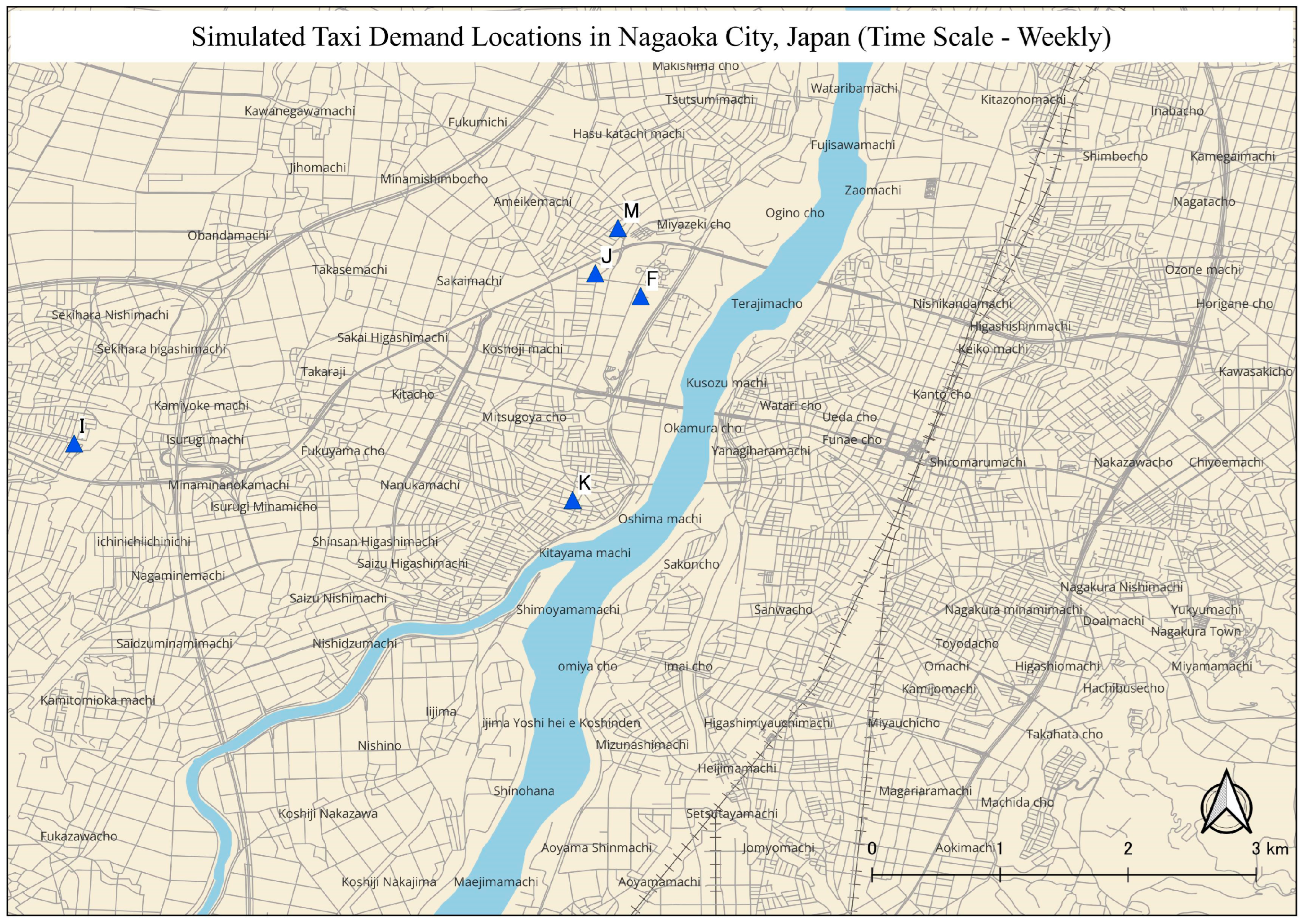
We analyze taxi Global Positioning System (GPS) data to detect taxi hotspots where drivers and passengers appear frequently in suburban areas. This research easily and formally identifies areas with high demand and quantifies those hotspots.
- (2)
We formulate a mathematical model of the taxi allocation problem to optimize the taxi drivers’ idle time costs as a mixed-integer program, which will support decision-makers, urban transport planners, and governmental and taxi companies to make their decisions more strategic. The proposed model focuses on taxis in suburban areas. Most of the existing studies, e.g., [
7,
33,
40], consider only the taxi model for urban areas other than suburban areas. Since the behavior of the taxi model for suburban areas is different from that of urban areas, our model can contribute to the reduction of CO
2 emissions and the efficient operation of a taxi service in suburban areas.
- (3)
We compare the performance of the proposed algorithm with two heuristic algorithms, namely greedy and simulated annealing. Further, we evaluate the optimality of the model by applying it to a real case study in Nagaoka City, Japan.
- (4)
Even though the recent articles [
33,
41] analyzed the CO
2 emissions in taxi operations, the optimization of the idle time and the number of taxis still needed to be considered. Therefore, this study focused on analyzing idle time and reducing taxi numbers to optimize taxi operations thus reducing CO
2 emissions.
4. Formulation of Mathematical Model
4.1. Establishing the Problem
The cost of taxi services is influenced by the idle time of the drivers, which is the time they spend without passengers. Idle time is not only unproductive but also increases fuel consumption and emissions. One way to reduce idle time is to match the supply and demand of taxis more efficiently by predicting where and when passengers will need a ride. For example, if a driver received a call from a nearby location, they would move towards it, but if the call were from a faraway or congested area, they would ignore it or decline it. This subsection presents the challenges of modeling the cost function that incorporates idle time and the benefits of using data-driven methods to optimize it. This way, we could capture the complexity and variability of the taxi service in our simulation.
By reducing the idle time, each taxi will have greater use, while the taxi driver spends less time finding passengers. Further, a smaller number of taxis can cover the same amount of demand. Accordingly, there are two objectives of this model:
To minimize the total idle time of the taxi driver when using the optimum number of allocated taxis.
To minimize the total operational cost when minimizing the idle time of the taxi driver and the number of taxis utilized of potential demand.
The above goals are directly tied to taxi system efficiency and driver profitability. In addition, idle time costs and the number of taxis can be considered important factors in reducing CO2 emissions.
4.2. Problem Assumptions
The following assumptions were used in this research to better understand the taxi problem:
Assumption 1—Passenger demand for taxis is assumed to be random:
This assumption highlights the importance of reducing idle time and optimizing routes to avoid unnecessary driving. Through the developed program, it is able to achieve significant reductions in both idle time and CO2 emissions while improving efficiency and reducing costs for all stakeholders involved.
Assumption 2—An empty car repeatedly moved over the planning horizon:
This assumption highlights the importance of reducing idle time and optimizing routes to avoid unnecessary driving. Through the developed program, is able to achieve significant reductions in both idle time and CO2 emissions, while improving efficiency and reducing costs for all stakeholders involved.
Assumption 3—The pick-up and drop-off must always happen within the specified time windows, i.e., the driver’s waiting time for the passengers and the passenger’s waiting time for the taxi.
Assumption (3) is the requirement for a successful taxi service to ensure that passengers’ pick-up and drop-off are done on time. It means that the drivers and the passengers must respect the agreed time windows for each trip, creating a more sustainable and efficient transportation system.
4.3. Formulation of the Idle Time Cost
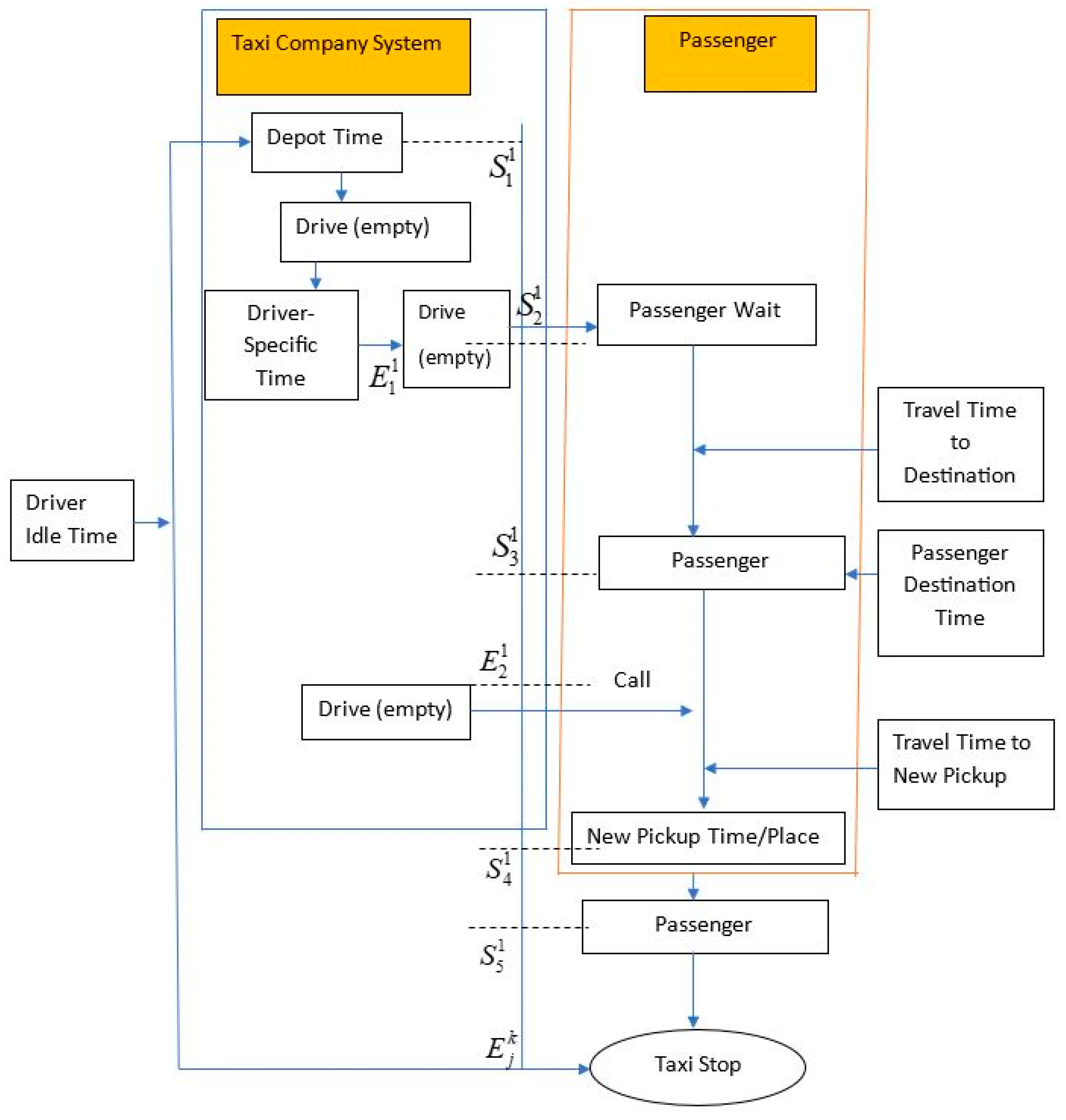
This paper shows a mathematical formulation of the taxi allocation problem for idle time cost. The present study considered an undirected graph that consists of locations and the A arcs (). Let and represent the start and end working times of the taxi driver at the locations and . For arc assign a positive distance and travel time . Location has a service time . The service time represents the time required for pick-up and drop-off, and the time indicates when the visit to the location must start. A taxi is allowed to arrive at a location before the start of the time, but it has to wait until the start of the time before the trip can be performed. The maximum capacity of a taxi is denoted by .
Figure 3 shows a sample of taxi allocation. This taxi (numbered 1 ∈ K) starts working time at location 1 at the time
. Location 1 is where this taxi remains stationed for passengers who are waiting. Then this taxi is assigned a passenger at the time
and moves to location 2 where the passenger is waiting. Then, this taxi pick-up the passenger at location 2 at the time
; after that, the onboard passenger drop-off at location 3 at the time
. After that, the driver waits at specific locations for the passenger, then the taxi is assigned a passenger at the time
and moves to new passenger pick-up location 4 at the time
and the onboard passenger drop-off location 5 at the time
. Idle time is defined as the amount of time a driver spends waiting for a new passenger request. Then, the total idle time can be calculated as
for this sample.
4.4. Formulations
The taxi driver idle time problem is formulated by several equations. Equation (1) develops from this study, and the flowing constraint functions are found in the previous literature surveys [
42].
The objective Function (1) minimizes the cost of taxi idle time and the number of taxis utilized of potential demand. is the idle time cost, which depends on the taxi company, but in this study, an idle time cost of JPY 300 has been used. Constraint (2) guarantees that the number of taxis coming to a passenger’s location and the number of taxis exiting are the same. Constraint (3) ensures that the taxi leaves the depot. Constraint (4) ensures that the taxi returns to the depot. Constraint (5) means that each passenger is riding only once in one taxi. Constraint (6) ensures that passengers do not consume more time at the taxi stand. Constraint (7) does not exceed the maximum capacity (Q). That means no more than one passenger per taxi. Constraint (8) is the binary condition.
5. Optimality Algorithms
The pick-up and drop-off problem is well-established as a non-deterministic polynomial-time hardness (NP-hard) problem, which means that the computational time required to solve it increases rapidly with the size of the expansion [
43,
44,
45]. This issue can be solved using two different algorithms. The first algorithm is an exact algorithm, and this is based on a mathematical model that guarantees the optimal result in every situation. The biggest disadvantage of this algorithm is the computing time necessary to solve the issue, particularly if it is NP-hard. The second algorithm is referred to as a set of heuristic algorithms, which use advanced mathematical optimization techniques such as branch-by-branch and neighborhood search.
Consequently, heuristic algorithms take less time to execute than accuracy algorithms. Although it has a quick processing time, the optimal solution is not guaranteed, and the results may not be satisfactory. This study utilized three types of heuristic techniques; construction heuristics, local search heuristics, and metaheuristics to derive a new heuristic algorithm.
This study utilized a linear mixed-integer programming model. Heuristic and metaheuristic algorithms can solve the model (1)–(8). Here devised a technique for solving the taxi issue that entails the establishment of (i) a greedy heuristic [
46], (ii) a local search [
46], (iii) a simulated annealing [
47] metaheuristic to solve the optimization problems, and (iv) a dynamic greedy algorithm to improve the greedy algorithm. The establishment of the detail of the algorithms is described in the following subsections.
5.1. Greedy Algorithm
The number of drivers, assignment costs, and the area that the first solution must have been all inputs to the heuristic method function. It begins by initializing all global parameters, such as the total number of passengers still requiring pick-up and drop-off, the global time, global distance, global service time, global waiting time, and total costs. The first iteration process begins when these variables are established, and it continues until all of the taxis available have been utilized. Once within the first iteration, the taxi driver parameters (i.e., total time, travel time, service time, waiting time, and costs) are set to their starting states, including the places that the taxi has previously chosen and its initial position and pick-up location. After collecting all pick-up sites from the passenger positions, the heuristic technique enters the second iterative step. This process continues until the present taxi runs out of drop-off sites or it is time to return to the depot.
It is common to use greedy heuristics to create effective initial solutions to difficult optimization problems. One can first, and sometimes intuitively, find an initial possible solution, which is subsequently improved by heuristics. To obtain a possible initial solution to the problem, an attractively structured heuristic is developed that considers the demand for all taxi stands and periods, prioritizes demand with high profit, and checks which taxis can be moved empty when necessary.
In the pseudocode presented for the greedy algorithm, the proposed greedy heuristic method is described as generating a relatively good initial solution to the taxi allocation problem. The basic idea is to check if there is a taxi that does not meet every pick-up that “arrives on time”. “Arrival time” refers to the travel time from the current location of pick-up within the requested time. It is also necessary to check whether the taxi route (empty or not) can be used to meet the demand.
We have taxi ride data for a set of drivers, and we want to optimize the idle time cost. Here is the greedy algorithm that would work:
Step 1: Start with an initial solution. This could be the initial sequence of rides for each taxi driver.
Step 2: Evaluate the cost of the initial solution. This would involve calculating the total idle time cost of all the taxi drivers.
Step 3: Determine the set of candidate solutions that can be obtained by making a small modification to the current solution. For example, we could consider swapping the order of two consecutive rides for a particular taxi driver.
Step 4: Evaluate the cost of each candidate solution. This would involve calculating the taxi drivers’ total idle time cost for each candidate solution.
Step 5: Select the candidate solution that provides the best immediate improvement in the objective function value and make it the new current solution. In this case, we want to minimize the total idle time cost of all the taxi drivers, so we would select the candidate solution that has the lowest idle time cost.
Step 6: If the stopping criterion is not met, repeat steps 3–5 until no more candidate solutions can be found or until the stopping criterion is met. The stopping criterion could be a maximum number of iterations or a minimum improvement in the objective function value.
Step 7: Return the current solution. The solution returned by the greedy algorithm would be the sequence of rides for each taxi driver that has the lowest total idle time cost.
The greedy works step-by-step based on the Algorithm 1 for optimizing idle time cost in taxi ride data.
| Algorithm 1: Greedy Heuristic |
| 1 | Function greedy |
| 2 | | Greedy solution = Solution () |
| 3 | | For each client in the total clients |
| 4 | | | Minimum costs = np.inf |
| 5 | | | Minimum costs driver = 0 |
| 6 | | | For each driver in the total drivers |
| 7 | | | | Current costs = calculate costs (client, driver, Greedy solution) |
| 8 | | | | | If the current costs < minimum costs |
| 9 | | | | | | Minimum costs driver = driver |
| 10 | | | | | | Minimum costs = current costs |
| 11 | | | Assert minimum costs driver! = 0 |
| 12 | | | Assign client (client, minimum costs driver, Greedy solution) |
| 13 | | Return all to depot (Greedy solution) |
| 14 | | Costs = total costs (Greedy solution) |
| 15 | | Greedy solution (total costs) = costs |
| 16 | | Assigned drivers = 0 |
| 17 | | For each driver in the total drivers |
| 18 | | | If the Greedy solution in the current driver assigned for each client |
| 19 | | | | Assigned drivers += 1 |
| 20 | Return Greedy solution |
| | | | | | | | | |
Taxi data (trip data) are input into memory. All empty and onboard passenger movement of the taxi is recorded in a data structure, including route, time, and cost. All passenger pick-ups are selected in sequential taxi calling, and if there are multiple pick-ups simultaneously, they are prioritized depending on the distance. The purpose of the problem is the value of the function. In the initial solution, the taxi driver calculates the cost of waiting time. It is the responsibility of the taxi driver if the current cost is less than the minimum cost. Finally, the optimal solution is evaluated by the greedy algorithm.
5.2. Local Search Strategy
Greedy developed an advanced method to perform from a greedy starting solution to investigate unmet pick-ups, which would be profitable. The local search method looks like the following. Here the steps of a local search algorithm are:
Step 1: Initialize the current solution to a random or heuristic solution.
Step 2: Evaluate the quality of the current solution using an objective function.
Step 3: Repeat the following steps until a stopping criterion is met:
- a.
Generate a neighboring solution by making a small perturbation to the current solution.
- b.
Evaluate the quality of the neighboring solution.
- c.
If the neighboring solution is better than the current one, accept it as the new one.
- d.
If the neighboring solution is worse than the current solution, accept it with a probability that depends on the difference in quality between the two solutions and the current temperature.
- e.
Update the temperature according to a cooling schedule.
Step 4: Return the best solution found during the search.
The following Algorithm 2 illustrates a basic outline of a local search algorithm, which can be used to solve various optimization problems. However, the specific implementation of the algorithm and the choice of the objective function, neighborhood structure, and cooling schedule depend on the problem being solved.
| Algorithm 2: Local Search Procedure |
| 1 | Function ImproveSolutions (Initial Route): |
| 2 | | Get local (no iteration) |
| 3 | | Current solution = randomly |
| 4 | | NUMBER ITERATION = no iteration |
| 5 | | Minimum cost = current solution (total costs) |
| 6 | | Values = zeros (no iteration) |
| 7 | | For each position in NUMBER ITERATION |
| 8 | | | New solution = neighbor (current solution) |
| 9 | | | If new solution (total costs) < minimum cost |
| 10 | | | | Minimum cost = new solution (total costs) |
| 11 | | | | Current solution = new solution |
| 12 | | | | Each position values = new solution (total costs) |
| 13 | | Assigned drivers = 0 |
| 14 | | For each position in the Number of drivers |
| 15 | | If current solution (each position of current driver assigned) |
| 16 | | | Assigned drivers += 1 |
| 17 | Return Current solution, Values |
| | | | | | | |
According to the solution of the model, a short-term scheduling model is developed using taxi driver information. Then it re-evaluates the costs for the two mentioned drivers, as this conversion does not affect the other drivers.
5.3. Simulated Annealing
The simulated annealing metaheuristic algorithm that was developed to solve the taxi allocation problem is described in the following steps.
Step 1: Start the program.
Step 2: Define the initial state or solution to the problem.
Step 3: Set the initial values for the algorithm’s parameters, such as the cooling rate and the number of iterations.
Step 4: Define the temperature schedule, which determines how the temperature changes over time.
Step 5: Generate a neighbor state or solution based on the current one. This is achieved by making a small change to the current state or solution.
Step 6: Calculate the energy or difference in cost between the current and neighbor solutions.
Step 7: Accept or reject the neighbor solution based on the energy or difference in cost and temperature. The neighbor solution is accepted if the energy is lower than the current energy. If the energy is higher, the neighbor solution is accepted with a certain probability that depends on the temperature.
Step 8: Repeat steps 5–7 until the temperature reaches a minimum value.
Step 9: End the program.
Simulated annealing is a stochastic relaxation method based on an iterative procedure starting from an initial “high temperature” with the system in a known configuration. The simulated annealing Algorithm 3 is a stochastic optimization algorithm that finds global optima by allowing uphill moves early in the optimization process. It achieves this by using a temperature parameter to determine the probability of accepting a worse solution. The iterative method of simulated annealing improves the cost function until the current temperature cools down. At high temperatures, atoms can become unstable from initial positions, meaning that the algorithm is allowed to have flexibility in searching potential space. In contrast, at decreasing temperatures, it is more likely to improve with local searches than with initial conditions.
| Algorithm 3: Simulated Annealing Procedure |
| 1 | Function Simulated Annealing (no iteration, low temperature, step, iteration step) |
| 2 | | Current solution = greedy solution |
| 3 | | Initial temperature |
| 4 | | For each step in the no iteration |
| 5 | | | Temperature solution = current solution |
| 6 | | | Cost delta = (temperature solution (total costs)–current solution (total costs))/current solution (total costs) |
| 7 | | | If cost delta <= 0 or random < exp (-cost delta / temperature) |
| 8 | | | | If temperature! = 0.1 or cost delta <= 0 |
| 9 | | | | | Current solution = temperature solution |
| 10 | | | | | Values (current solution (total costs)) |
| 11 | | | If each step % iteration step == 0 and temperature > low temperature +
1e-10: |
| 12 | | | | Temperature−= each step |
| 13 | Return Current solution, values |
| | | | | | | |
Simulated annealing is a potential method that is proposed to find a global minimum cost function that may contain several minimums [
48]. By updating the model, optimizers link the cost function and model parameters together in order to achieve global minima with respect to the cost function. The objective is to minimize the cost function of the taxi system, while the search for the best solution refers to the cooling process.
5.4. Dynamic Greedy Programming
In dynamic greedy programming, decisions are made by considering the current problem and the solutions of previously solved subproblems to compute the best solution. This makes it the best solution because it considers all possible cases and chooses the best. For dynamic programming implementation, an additional data structure must be created. Here is a step-by-step explanation of the dynamic greedy algorithm based on the flowchart:
Step 1: Start the program.
Step 2: Define the problem that needs to be solved. This involves specifying the inputs, the objective function to be optimized, and any constraints that need to be satisfied.
Step 3: Divide the problem into smaller subproblems that can be solved independently. This is achieved using dynamic programming. The subproblems are usually defined in terms of a sequence of decisions or states that need to be made or reached to obtain the optimal solution.
Step 4: Solve each subproblem using the greedy algorithm. The greedy algorithm makes the locally optimal choice at each decision point in the subproblem. This means that it chooses the option that provides the maximum benefit at that particular point in time without considering the long-term consequences of that choice.
Step 5: Combine the solutions to the subproblems to obtain a solution to the original problem. This is achieved using dynamic programming. The solutions to the subproblems are combined to obtain the optimal solution to the original problem. This is achieved by choosing the sequence of decisions or states that provide the maximum benefit overall.
Step 6: Repeat steps 3–5 until an optimal solution is found. The dynamic greedy algorithm iteratively solves the subproblems and combines the solutions until an optimal solution is obtained. This involves solving the subproblems in a sequence that allows the maximum benefit to be achieved overall.
Step 7: End the program. The dynamic greedy algorithm terminates once the optimal solution has been obtained.
In summary, the dynamic greedy Algorithm 4 is an iterative process that uses dynamic programming and the greedy algorithm to obtain an optimal solution to a problem that involves a sequence of decisions or states.
| Algorithm 4: Dynamic Greedy Procedure |
| 1 | Function DynamicGreedySolution |
| 2 | | For each client in the total clients |
| 3 | | | Minimum cost = np.inf |
| 4 | | | Minimum driver = 0 |
| 5 | | | Time of minimum driver = 0 |
| 6 | | | For each driver in the total driver |
| 7 | | | | Distance to client = distance (client, driver) |
| 8 | | | | Time on arrive to the client = maximum (client desired time, distance to client/speed + driver time) |
| 9 | | | | Lateness = time on arrive to the client–client desired time |
| 10 | | | | Idle cost = lateness ** 2 + time on arrive to the client + client segment |
| 11 | | | | | If drivers == 0: |
| 12 | | | | | | Idle += driver opening cost |
| 13 | | | | | If minimum cost > idle cost |
| 14 | | | | | | Minimum cost = idle cost |
| 15 | | | | | | Minimum driver = driver |
| 16 | | | | | | Time minimum driver = time on arrive to the client |
| 17 | Driver cost [minimum driver] += minimum cost |
| 18 | Drivers on [minimum diver] = 1.0 |
| 19 | Driver position [minimum driver] = client position |
| 20 | Driver time [minimum driver] = time min driver + client segment/speed |
| 21 | Minimum costs of drivers |
For this purpose, greedy and dynamic are combined into the dynamic greedy algorithm. The optimization method is applied in dynamic greedy programming, and the minimum total cost is found.
6. Results and Discussion
This section shows the results of the experiments for the performance of the proposed algorithms. The proposed mathematical model is solved by three algorithms shown in
Section 5. The total number of taxis (42) means the number of taxis in the company. The heuristics were written in the Python programming language. The tests were carried out using a laptop with an Intel (R) Core (TM) i7-5500U CPU running at 2.40 GHz, with 16 GB of RAM, and using the Windows 10 operating system.
The dataset has three instances, 01.01.19, 01.03.19, and 15.03.19, representing taxi problems in Nagaoka City. These instances contain between 333 and 658 passenger demand. Additionally, there are problems where only a subset of the taxi fleet can serve the passenger requests. To make it easier for the heuristic to find solutions, we set the number of available vehicles to one more than required. According to the model, taxi demand was the optimized number of taxis (approximately 8) that was sufficient for a day.
Table 4 presents the average passenger demand, the number of taxis, the total cost, and the CPU time calculated for each algorithm. The outcomes are based on randomly generated taxi demand situations. The greedy, simulated annealing, and dynamic greedy heuristics showed average total costs of JPY 21,433.93, JPY 23,730.75, and JPY 20,573.98, respectively, in the optimal solution. The dynamic greedy heuristic required an average CPU time of 1.19 s to find the optimal solutions. The findings show it was able to identify better solutions in a shorter period on the CPU.
The lengthy simulated annealing schedule may take a while to complete. The beginning and finishing temperatures for the simulated annealing were set as 0.21. The decay rate was 0.001. These parameters were maintained for all problems and independent runs. Each problem was solved 10 times by using an iteration step of 500, with the initial step of 0.1 and a low temperature of 0.1. Further, simulated annealing has a lot of adjustable parameters. Therefore, simulated annealing takes comparatively longer CPU time for simulation. On the other hand, the greedy algorithm also consumes comparatively longer time since it breaks the issue into its components and remembers the answer for each element to apply it later when a similar component occurs again. Compared to other algorithms, dynamic greedy algorithms have lower temporal complexity and identify the most practical solution to arrive at the best solution at every stage. Therefore, dynamic greedy algorithms consume comparatively less time for the simulation process.
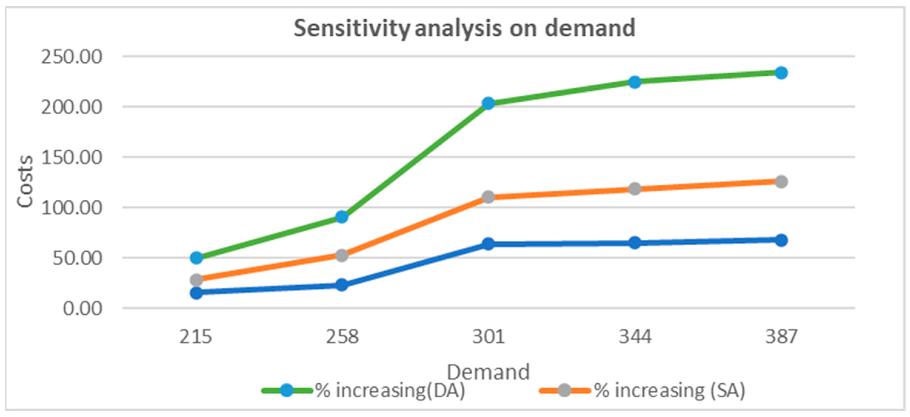
The passenger demand/per day for the suburban area of Nagaoka City is, on average, 509, with the average number of taxis required as 8. The optimization results of the taxi allocation problem with different demands are summarized in
Table 4. As the demand increased, the total idle time costs increased from JPY 10,548.54 with five taxis to JPY 28,292.11 with ten taxis in the greedy algorithm, and in the simulated annealing algorithm from JPY 13,883.37 to JPY 31,005.28. However, the proposed algorithm (dynamic greedy algorithm) increased the cost from JPY 9175.24 to JPY 27,944.63.
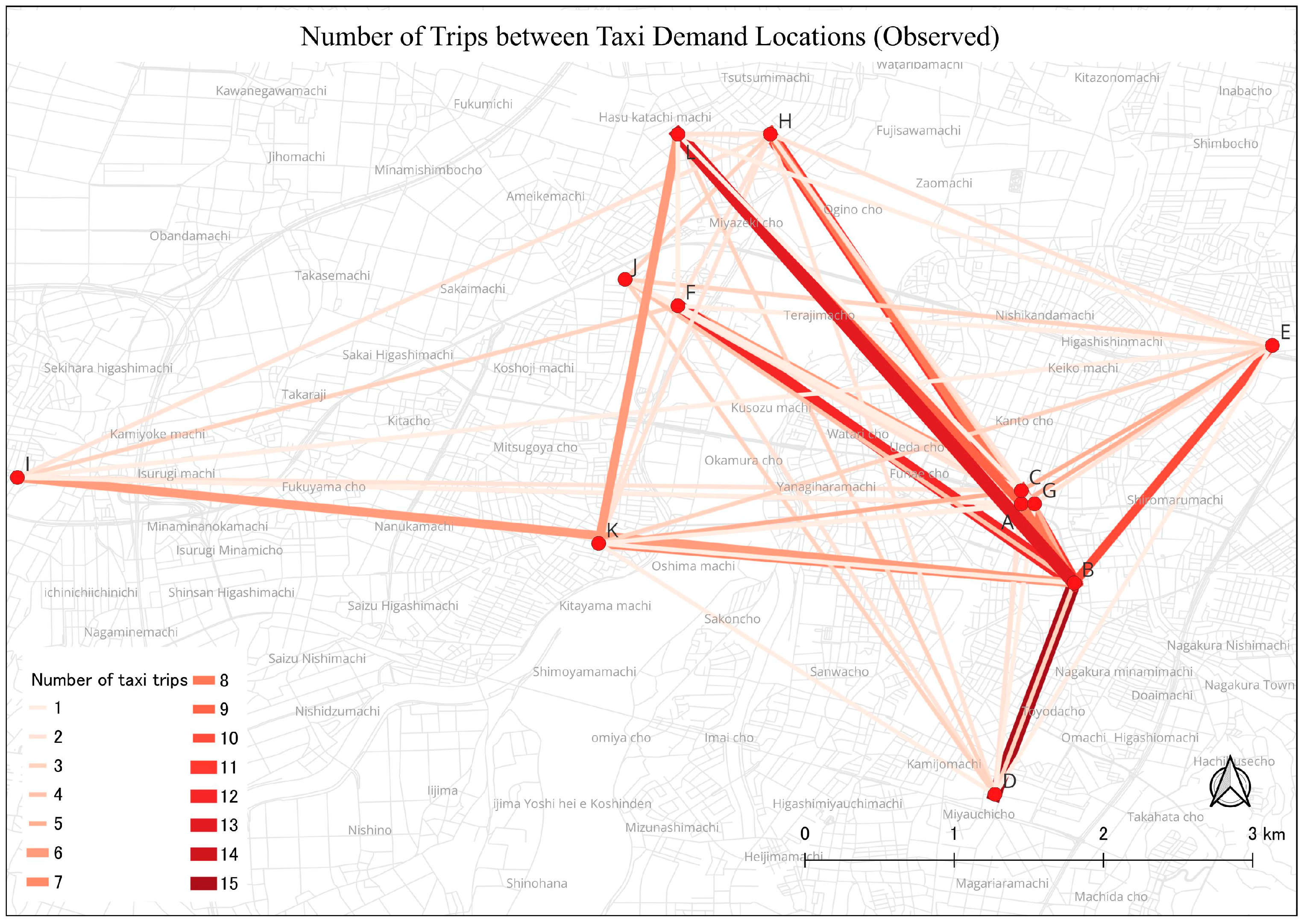
In addition, a dataset with information on taxi trips, including pick-up and drop-off locations, was examined. This investigated the pick-up and drop-off coordinates from the dataset and used them to compile the taxi trips for each location. This paper combined the trips based on these coordinates to determine how frequently taxis picked up and dropped off passengers at each distinct place.
Figure 4 represents the regular average of 509 taxi trips per day in Nagaoka City.
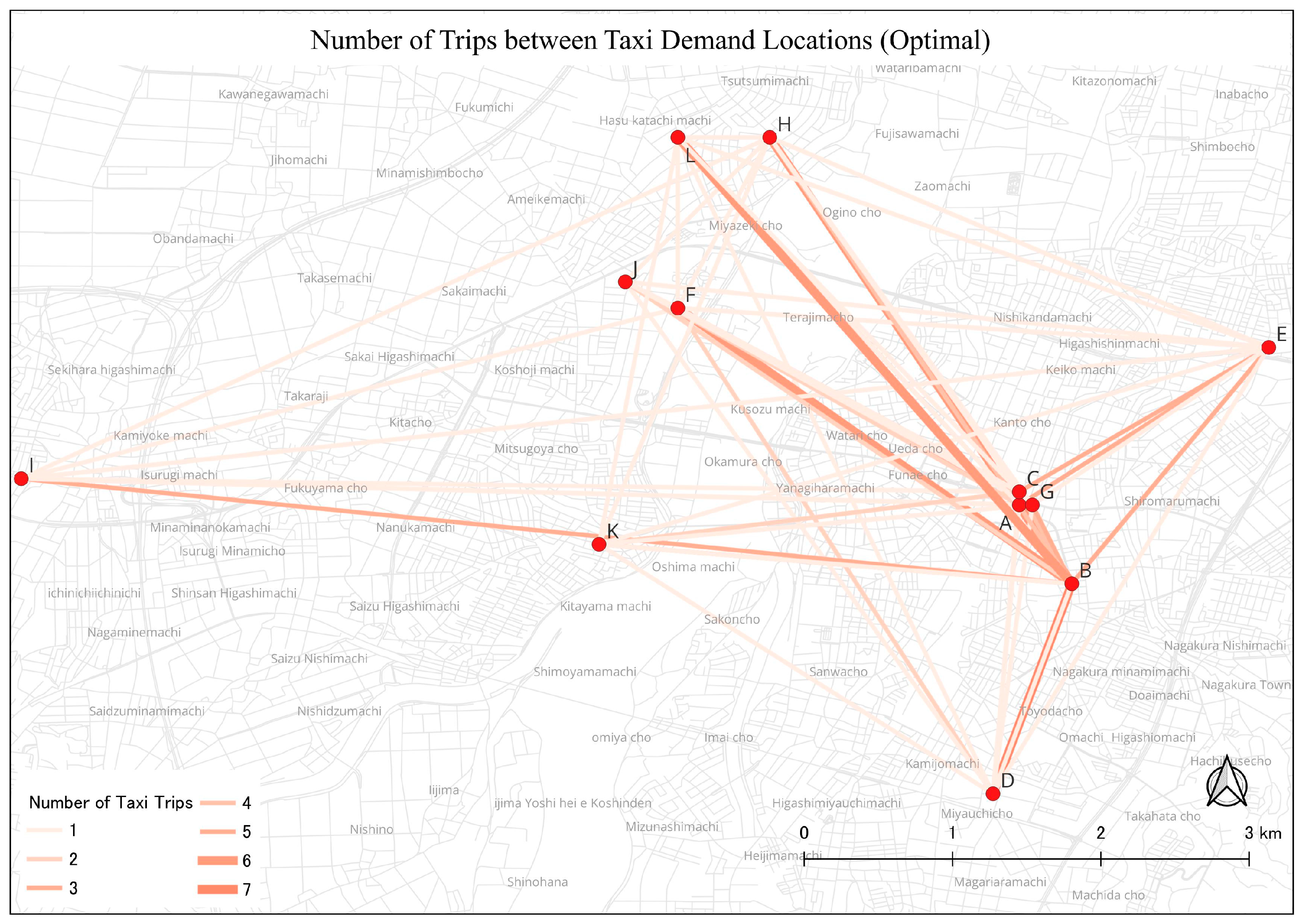
The number of journeys was reduced, and it was determined which trips showed notable drops. The dataset reflects the taxi journeys across several places by integrating and preprocessing these various datasets. The proposed model was obtained to optimize taxi driver idle time, taxi routes, and allocations while taking into account parameters including trip distances, traffic conditions, and passenger demand (
Figure 5). After solving, the model reduced the overall number of trips while preserving effective transportation services by redefining the issue as an optimization challenge. The fact that the number of trips fell by a statistically significant amount shows that the model was successful in optimizing the taxi service and maximizing resource usage. This result implies that the model was successful in identifying chances for trip consolidation, whereby a number of passengers with comparable itineraries were put together, resulting in fewer individual journeys.
The results of this study have implications that the reduction in taxi trips indicates the potential for improved efficiency and sustainability in suburban transportation systems. By optimizing route planning and allocation of resources, the number of unnecessary trips has been minimized, which leads to reduced fuel consumption, and CO2 emissions.
Calculate the Total CO2 Emissions
The emission factor for taxis can vary depending on the type of vehicle, the fuel type, and the average distance traveled. According to the U.S. Environmental Protection Agency (EPA), the average CO
2 emissions for a gasoline-powered taxi is approximately 0.404 kg/mile [
49]. Using the carbon footprint model [
50] provides a useful starting point for understanding the environmental impact of the taxi fleet and identifying ways to reduce emissions. The carbon footprint model is as follows:
where
: the number of allocated taxis per day,
Minimizing the number of taxis required to serve all passenger demand is typically the top priority in this problem. The current heuristic approach addresses this objective by proposing a simple algorithm that minimizes the number of vehicles needed. It is worth noting that the algorithm is only suitable for problems involving a homogeneous fleet of taxis. We also assume that the number of taxis available is 42, so constructing an initial feasible solution can always be done. This paper focused on minimizing the CO2 emissions from taxi idle time and reducing the number of taxis that idle. This can be achieved by implementing policies or practices that encourage drivers to turn off their engines when not driving, such as turning off the engine during short breaks or when waiting for passengers.
The number of allocated taxis per day is 42 taxis that the company used and the average CO
2 emissions per taxi are 0.404 kg/mile. Each taxi travels an average of 64.10 miles per day, then from Equation (9), the total daily CO
2 emissions from the taxi would be:
After the optimal solution of the mathematical model in the case study, we minimize the number of taxis and costs. On average, the number of taxis per day used is only 8 in
Table 4. Therefore, the total daily CO
2 emissions are:
The taxis in the suburban area of Nagaoka have reduced their CO2 emissions by 81.84%, which amounts to 890.17 kg per day.
This paper presents a novel model for optimizing the operations of a taxi firm using a simulation-based approach to evaluate the performance of our model. It shows that our model can effectively capture the real-world situation of the taxi market. By using the proposed model, the best number of taxi hours can be made available to customers while retaining driver benefits, which means reducing customer waiting time and making it one of the best solutions. The effects on taxi customers must be taken into account when researching reducing taxi operating costs.
Table 4 shows the optimal allocation of taxi demand. This confirms that the model can minimize the total idle time costs of taxi drivers while minimizing CO
2 emission. Dynamic greedy heuristics in a relatively short runtime successfully solved the taxi allocation problem, making this an effective tool for taxi companies.
Taxi companies should know that establishing a decision support system will benefit fleet management and empty taxi repositioning. The results of our case study on optimizing taxi allocation and minimizing CO
2 emissions in a suburban area were very encouraging. By collecting and analyzing data on taxi usage patterns, it is able to identify areas of high demand and optimize taxi allocation to reduce idle time, which in turn leads to a reduction in CO
2 emissions. Optimization algorithms to identify the most efficient routes for taxis also significantly reduced the distance traveled by taxis and the amount of CO
2 emissions produced. This was achieved by minimizing the number of empty trips and optimizing routes to avoid traffic congestion. The existing studies [
8,
33] described their model could reduce CO
2 emissions from 36% to 47.62% in urban areas, whereas this proposed model could reduce CO
2 emissions up to 81.84 % in suburban areas. Therefore, this model can make a sufficient contribution to the reduction of CO
2 emissions.
Taxi drivers and passengers saved time and money, while the suburban area became more sustainable and environmentally friendly. The success of this case study highlights the potential for similar programs to be implemented in other regions and cities. Using data analysis, optimization algorithms, and incentives can create a more sustainable and efficient transportation system that benefits everyone involved. It also highlights the importance of taking action to reduce CO2 emissions and mitigate the impact of climate change.
8. Conclusions
Efficient transportation systems are necessary to reduce CO2 emissions in the context of climate change. Taxi services are an essential part of the transportation system in urban and rural areas. Inefficient taxi services cause problems such as increased idle times, resulting in increased CO2 emissions. Therefore, optimizing taxi allocation can help reduce CO2 emissions and improve the sustainability of urban transportation. For this purpose, this study proposed a mathematical model of taxi allocation optimization problem for minimizing taxi driver idle time costs which help to reduce CO2 emission in suburban contexts. Since the proposed model is formulated as a mixed-integer program, it is necessary to propose the solution algorithm as well. We proposed three heuristic algorithms: greedy algorithm, simulated annealing algorithm, and dynamic greedy. Further, a case study has been carried out to demonstrate the proposed methods and show its implication by using real taxi data from Nagaoka, Japan. For the case study, we first identified the taxi travel hotspots as potential locations for taxi spots by investigating the pick-up and drop-off locations and times by analyzing the GPS data of the taxi. After that, we found the optimal taxi allocations by applying the proposed model and solution algorithms. To summarize, dynamic greedy heuristics successfully obtained excellent solutions in relatively short runtimes for the taxi issue, making strategic decisions and feasible choices for taxi markets to adopt. The case study application in this study demonstrates the potential for using data analysis, optimization of taxi allocations and the number of taxis, and reducing approximately 81.84% of CO2 emissions in the transportation sector. Finally, sensitivity analysis was applied to validate the model for passenger demand. The sensitivity analysis showed that the total idle time cost increased if the demand increased.
To conclude, the optimization of taxi allocations can have a significant impact on creating carbon-free and environmentally friendly cities. By strategically placing taxi spots and optimizing their routes, cities can reduce the number of vehicles on the road, decreasing harmful emissions and improving air quality. Therefore, it is essential for cities to invest in and prioritize taxi allocation optimization as a crucial step toward achieving sustainable transportation. Future research able to be conducted utilizing machine learning algorithms to solve the allocation issue may provide promising results. This model can also be adapted to improve the performance of taxis in various cities and other urban public transport networks.


