1. Introduction
Nowadays, dynamic pricing methods are widely used in e-commerce online services for marketplaces, transport/sports/entertainment ticket sales, and hotel/car/equipment booking AI systems [
1,
2,
3,
4,
5]. Roughly speaking, these methods build a strategy for maximizing business profit, revenue, or conversion by setting flexible prices for products or services based on current market demand and supply, competitor pricing, and other internal and external factors. The operating principles of dynamic pricing industrial systems usually remain hidden as a commercial secret. However, based on the advertising information of such systems [
6,
7,
8,
9,
10], it is natural to suppose that they are complex models of real purchasing processes that possibly take into account numerous features (such as weather, seasonality, event calendar, consumer behavior, etc.) and exploit deep learning or other advanced technologies; see, e.g., the descriptions in [
6,
7,
8,
9,
10]. Recall that dynamic pricing methods usually rely on the price elasticity of demand model, which is built based on available historical data.
Note that there are two types of strategies for the dynamical setting of prices used in AI e-commerce systems. The first one is for ordinary products, goods, and services. In this case, the dynamics are often controlled only by external factors (such as weather, calendar, etc.). The second and more interesting type is specifically for ticket systems (such as transport, mass events, etc.), which are designed to reflect demand before the upcoming event. In this case, the dynamics are determined mainly by internal factors (such as the number of tickets sold) and are indeed available for management (such as in the process of solving the conversion maximization problem). In this regard, we will further discuss the dynamic pricing for ticket systems.
Dynamic pricing strategies inside of these systems are effective tools used to manage population mobility. When alternative carriers, routes, or modes of transportation exist, the pricing strategies of carriers create an opaque picture of human mobility and transportation accessibility. The standard models of mobility, such as minimizing distance or travel time, or gravity models, are no longer sufficient for explaining this picture. Therefore, a scientific tool is needed to provide a deep understanding of carrier dynamic pricing strategies in order to (a) evaluate and predict their impact on mobility, (b) identify collective effects of carrier interactions (competition and collaboration), and (c) optimize various processes from individual carrier profit to the satisfaction of a particular region population with the quality of carrier services. In this paper, a method for restoring a dynamic pricing strategy based on open data for a single carrier is proposed. This method can be used both for carrier operation optimization (as shown in the paper) and solving other tasks mentioned above, highlighting the study’s importance.
From the scientific side, it seems that the existing dynamic pricing methods described in publications often lack a common performance evaluation methodology, appropriate public data, and source code, making them hardly reproducible in this sense (one can check, for example, the works [
11,
12,
13,
14] on these issues; see also
Table 1 below). The lack of a common, generally accepted evaluation methodology, among other things, may be because the authors of publications often focus on solving their particular dynamic pricing problems for non-public data, such as price elasticity of demand approximation [
3,
15,
16,
17,
18,
19,
20], consumer behavior analysis [
21], price optimization [
12,
22], and others. As a result, the scientific field lacks reproducible studies where dynamic pricing methods are compared with each other in a unified manner.
Since today’s markets are highly competitive, the question often arises as to how a company should evaluate its dynamic pricing system against competitor systems. In this regard, the problem of the quality ranking of existing methods for a dynamic adjustment of prices on public data can be stated. It is reasonable to suppose that the solution to this problem may be based on the use of a data-driven method that first builds a surrogate price elasticity of demand model [
27] using the public data generated by the hidden company’s dynamic pricing model and further applies the surrogate model to build an exposed model of dynamic pricing. The hidden and exposed models may be further compared systematically in terms of quality performance; for example, by using a Monte Carlo simulation method (e.g., in terms of the company’s revenue from sales based on a dynamic adjustment of prices). In our study, we propose such a method and show that it is indeed suitable for comparing the quality performance of the hidden and exposed models, thus indicating the potential for improving the existing (hidden to us) company’s dynamic pricing model.
In this regard, the following tasks were set for this study:
Building a surrogate price elasticity of demand model only on the basis of public data (generated by the hidden dynamic pricing model) of a commercial company;
Interpreting and analyzing the quality of the developed model;
Building an exposed dynamic pricing model within an optimization procedure using the built price elasticity of demand model;
Developing a systematic quality ranking method for a comparison of the hidden and exposed dynamic pricing models.
The main feature of our surrogate price elasticity of demand model is that it uses simple data approximants (oppositely to complex commercial methods). In order to build the exposed model, the surrogate model in a multi-class constrained optimization procedure was used to maximize the company’s revenue using an evolutionary algorithm. The quality evaluation method is based on the Monte Carlo method and produces revenue estimates. Thus, a systematic method is proposed that allows one to conduct comparison experiments for existing (hidden to us) dynamic pricing methods in a unified manner.
Note that a framework for crawling an open Internet data was created by us, which allows us to collect a dataset from a Russian railway passenger carrier company for a period from 12 April 2021 to 17 March 2022 (1,105,025 records, approximately 29 trains in total). The effectiveness of the method was tested on this data, while, in the paper, the examples are given only for the 11 most diverse trains from Moscow to St. Petersburg. In order to increase reproducibility in the field, our data, source code, and results are presented on GitHub (
https://github.com/AlgoMathITMO/DPRank, accessed on 7 May 2023). We call our method
DPRank, which stands for
Dynamic
Pricing
Ranking.
This paper is organized as follows:
Section 2 is devoted to a discussion of existing research on the topic;
Section 3 describes the proposed method for dynamic pricing quality evaluation in mathematical details;
Section 4 is about the experiments performed using the proposed method.
2. Literature Review
As was already mentioned, the operating principles of dynamic pricing methods that are widely used in e-commerce online services for marketplaces, ticket sales, and booking systems [
1,
2] usually stay hidden as a commercial secret. The situation in the scientific area is not much better: it seems that the existing dynamic pricing methods described in publications often have a lack of a generally accepted quality evaluation and comparison methodology, public data, and source code; see
Table 1 for studies considering existing methods for trains. (In
Table 1, the sign
indicates that the data-driven dynamic pricing comparison is only carried out in a simulated environment. In addition, the sign
indicates that the data-driven comparison is performed between the revenue value obtained by the dynamic pricing method proposed and a fixed revenue value given). As a result, the scientific field suffers from a lack of reproducible studies where dynamic pricing methods are compared with each other in a unified way. There is a discussion of the most related studies in a more detailed manner below.
A variant of a solution to the data-driven dynamic pricing problem as an optimization problem with a parametrically specified demand was proposed in Ref. [
27]. The authors considered in detail the cases of dynamic pricing with and without competition and compared the calculated results for a myopic pricing policy and a one-dimensional and multidimensional dynamic programming formulation of the pricing problem. Note that the authors used classical statistical tools for data-driven modeling.
A number of authors provide solutions to the dynamic pricing problem for the sphere of passenger transportation, namely in the railway, aviation, and automotive sectors of companies. In the rail industry, there is the study [
22] on dynamic pricing for high-speed trains that proposes the use of two demand functions and sets a revenue maximization optimization problem that takes into account price constraints. Features of passenger behavior are considered in several studies, e.g., in Refs. [
3,
18,
23], while the distribution of changes in the railway carriage capacity is discussed in Refs. [
19,
24]. The authors of Ref. [
12] considered the solution to the dynamic pricing problem using a linear regression model for high-speed rail transportation in an imperfectly competitive market with a short-sighted pricing policy of demand and one passenger service class. Dynamic pricing in the context of demand forecasting is considered, e.g., in Refs. [
13,
14].
There are two works [
25,
26] where the authors solve the revenue maximization task using nonlinear programming methods. In Ref. [
25], the demand intensity was modeled by a neural network model based on seasonal features, while, in Ref. [
26], the ticket-purchasing process was described via a Poisson process.
There are also a number of studies devoted to the dynamic forecasting of railway ticket prices by taking into account historical data, including the number of days before departure and the day of the train departure week [
28,
29]. In order to predict demand, researchers often use linear regression and gradient boosting [
15,
30], and a random forest algorithm [
17].
Note that a survey covering applications of artificial intelligence in railway services [
31] exists. In particular, the topic of dynamic pricing is briefly covered there.
The sphere of dynamic pricing for air transportation is more widely studied than for railway transportation. For example, the authors of Refs. [
16,
20] suggested the use of neural networks for demand forecasting using historical data. An analysis of an air transportation market with a comparison of prices for local and international flights was proposed in Ref. [
21]. A comparison of approximating algorithms was performed in Ref. [
32]. Two-stage dynamic pricing using neural networks and optimization was proposed in Ref. [
33].
One of the least studied dynamic pricing area is the field of bus transportation. The works [
1,
2] describe dynamic pricing and price forecasting for intercity buses, where price dynamics are studied among other things. The authors note that it is important to take into account the day of the week, time, distance of the trip, and the possibility of booking tickets before the trip.
Note that there is a work on optimization algorithms and their features [
34], as well as a work [
35] on time series forecasting (both in relation to dynamic pricing) for railway tickets using data obtained from Google trends. These works may be useful for understanding the practical aspects of the problems one may face during solving the dynamic pricing problem. As for optimization methods from other fields of study, we can find a similar problem in papers [
36,
37]. The authors of these papers solved the tasks of medical supplies delivery and the management of electricity system optimization, respectively. However, these problems differ from ours in that they address multi-objective optimization.
Returning to dynamic pricing for trains and the papers listed in
Table 1, one can notice that there is only one work [
3] where a data-driven comparison of several methods is performed. However, the experiments were conducted in a simulated environment, which was based on data about a railway network containing information about stations, itineraries, and schedules. The customer behavior in this simulation was not based on any open public dynamic pricing data. Furthermore, two works [
18,
24] performed data-driven comparisons between the proposed dynamic pricing method and (a) the revenue obtained with fixed fares and (b) the average value of ticket revenue for several trains. Unfortunately, even these three papers, which may be considered the most similar to our methodology, are not reproducible due to the lack of publicly available data and code.
Before the description of our method in detail, one should note that it follows the general methodology in the field, particularly by using classical statistical tools for data-driven modeling, similar to [
27]. However, the proposed scheme can be found particularly useful for its application and unification of the field as it provides a reproducible, systematic, methodological approach for evaluating the quality of dynamic pricing models exclusively using open public data, and experimentally demonstrates how it can be used to identify potential improvements in the existing (hidden) company’s model.
3. Mathematical Description of Our Method
3.1. Notation for Public Data Processing
Note that the data are usually publicly available on online ticket systems that use dynamic pricing models hidden to us [
4,
6]. In this study, we supposed that the data are parsed from the system once per day, at the same chosen time. The aim is to observe what happens with prices and available tickets in order to analyze how the corresponding dynamic pricing process is working.
Note that the goal is to provide a unified notation below that is still suitable for the transportation company data one will deal with in the experimental study. The main notation is collected in
Table 2 and
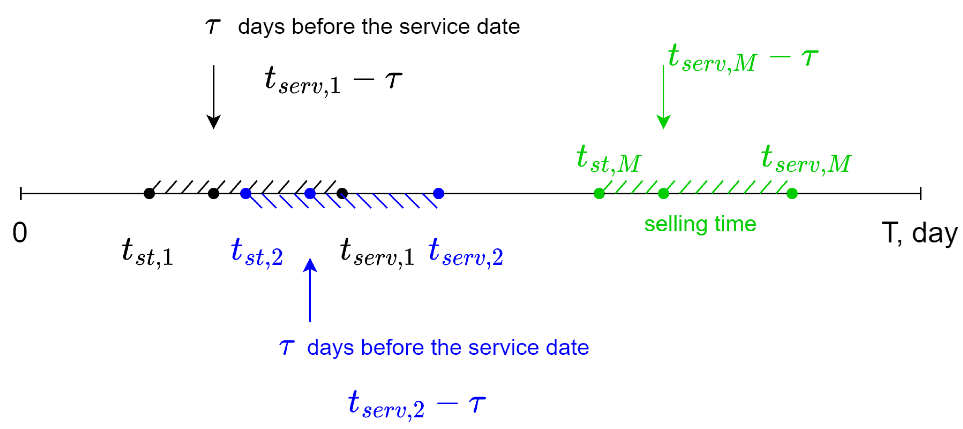
Figure 1.
First, suppose that the online ticket system is observed for a fixed period of time
; see
Figure 1. It is possible that the service can be provided during this period several times; say,
, a fixed number. Furthermore, the system may start selling the tickets several times too. For simplicity, let the number of selling time periods (that may overlap) in
be the same positive integer
M as in
Figure 1. Thus, each selling time period can be numbered with
. The selling start and service date (the selling end) are denoted as
and
, respectively. Note that it is also supposed that
is the same for each
m. In each selling time period, data can be collected
days before the service date
so that the sequence
is decreasing down to
.
For example, if one works with a train ticket selling system, then, according to the above-mentioned terms, one can check days in advance the price and number of available train tickets for a chosen train that departs on a specific date.
Furthermore, the type of service (ticket) is also important (as there may be several types). Suppose that there are service classes and let us number the classes by . If one considers a chosen service, k, it can be thought of as fixed and so one performs below by skipping k in indexes (before one comes to the multiclass optimization procedure).
Thus, only
m and
change, with all other parameters fixed. For them, in the online ticket system,
can be observed, which is the price of the ticket that may be bought
days before the service date
for the service of class
k.One can also observe
, the number of available tickets with the price
. If one considers only
, where
is an increasing sequence of days in the selling period
m when at least one ticket is sold, then the data available are
For simplicity, it is supposed that the whole number of tickets available for the service chosen is fixed and that no-one can return a ticket once it is bought (this is not the case in real-world online ticket systems and therefore we will have to cope with it in the experimental study). This means that the number of available tickets is non-increasing up to the service date and thus the sequence is non-decreasing with respect to running over .
3.2. Hidden Price
Elasticity of Demand and Dynamic Pricing Models
The data (
2) are not yet suitable for building the price elasticity of demand model as it requires the demand value and not the number of tickets available. Under the assumptions of
, demand
(of the service with the price
if at least 1 ticket is sold in the day
) can be easily calculated as
Recall that the number of available tickets
days before the service is at least the number of available tickets
days before the service plus 1 (by construction); see also
Figure 1.
In this way, instead of (
2), we obtain
under the assumption that the service class
k is fixed (otherwise one needs to add the corresponding indexes).
Having all the above-mention terms at hand, one can assume that the hidden price elasticity of demand model [
27]
used in the hidden dynamic pricing model
for each
is as follows:
for the data (
4). In (
5), ⋯ means other possible arguments, including exogenous variables, random components, etc.
3.3. Surrogate Price
Elasticity of Demand Model
The purpose now is to build a surrogate price elasticity of demand model
using only the public data (
4) and to further apply the model to build our exposed dynamic pricing model
. In order to build
, simple data approximants such as linear or power, with additional random components, are used [
12,
18,
19,
27]. As usual, it is supposed that, when the price rises, the quantity demanded decreases for the service chosen. Motivated by the preliminary patterns found in the data used in our experimental study, here, a power (the log-linear option is chosen, e.g., in [
12,
18,
19,
27]; however, the data there remain unpublished, and thus it is hardly possible to evaluate the choice)
for each
of the form is chosen:
where
are unknown coefficients and
is the relative error of the model. Here,
as
and
because the demand is expected to decrease while the price increases. Furthermore,
of the form in (
6) is taken in order to translate the data (
4) to the origin and to avoid the singularity supposing that
and that the demand for the minimal price (over
) is at least 1.
Recall that the coefficients
and
for the data (
4) can be easily found by taking the logarithm of both parts of (
6) that are well-defined by the construction of (
4) and solving the linear approximation problem for the (correspondingly modified) data using the model
by means of least squares. In (
7),
and
are now unknown coefficients and
is the absolute error of the linear model. Namely, for the period
and
, a unique solution to the following optimization problem for each
that has to be found is provided:
where
and
are from (
4).
Note that one usually works in the presence of data streams when it is necessary to update the model built when new data are coming [
38,
39]. The model (
6) is rather convenient in this sense; see
Appendix A.
3.4. Empirical Relative Frequency Distribution Used in Monte Carlo Simulation
Furthermore, one can find the absolute model’s error for each
by (
7) and thus build the empirical relative frequency distribution, eRFD, for
, and further connect it with the eRFD of
in (
6). In what follows, the latter is called
, i.e.,
The eCDFs will further be used in the Monte-Carlo simulation.
3.5. Exposed Dynamic Pricing (Price Optimization) Model
Thus, the surrogate price elasticity of demand model
is built by the data (
4). Now, it is applied to build the exposed dynamic pricing model
.
As usually performed, the company’s ticket sale revenue for the period
for
K classes is used as an objective function:
where
is a pricing strategy, i.e., the set of
, the prices
days before the service date
in the selling time period
m of tickets of class
k. Furthermore,
in (
10) is the surrogate price elasticity of demand function from (
6). The optimization problem then may be stated as follows: find
, which is a solution to
under the following demand and price constraints (inferred from the data (
4)):
where
is the average capacity (number of tickets) and
is the interval of price values allowed for class
k in the period
. (It should be noted that the constraints are rather flexible and that, by varying the constraints, one can change the pricing strategy.) The upper bound on demand does not allow the optimizer to offer more tickets for sale than the company had on average in
.
Thus, the
model for the period
is based on a solution
to (
11) with constraints (
12), where (
10) is based on the SEd model (
6).
3.6. Monte Carlo Simulation
Recall that there is a random component in (
6) and thus the
model may produce different
over runs of a Monte Carlo simulation. For instance, if it is simulated
J times, the corresponding revenues may be represented as
Analogously to (
10) but without optimization already, the revenue for the hidden dynamic pricing model,
, can be found from the data (
4) for the same period
:
As a result, once and are found, the corresponding dynamic pricing models’ quality performance can be compared. For example, we can find the difference between and the mean value of the elements of . This quality performance difference (in terms of the company’s revenue from ticket sales) between the hidden and exposed models indicates the potential for improving the existing (hidden to us) company’s dynamic pricing model.
Note that the above-mentioned optimization can be performed by different numerical methods. In our experimental study, a differential evolution algorithm was applied.
3.7. Demand, Price, and Revenue Estimation and Comparison of Dynamic Pricing Models
The hidden and exposed dynamic pricing models were then compared by means of confidence intervals for price, demand, and revenue, obtained within the Monte-Carlo simulation.
In order to estimate the confidence interval characterizing the prices obtained from the hidden model with the confidence level
and the sample size
n, one should calculate for
the mathematical expectation
and the corresponding unbiased estimate of the standard deviation
:
where
is the 95th percentile of the Student’s distribution with
degrees of freedom.
At the same time, the standard deviation of prices for services is formed due to the spread of prices for all services of this type, which are paid days before the services, for each kth service class separately.
The confidence interval for demand and revenue has the form analogous to (
15).
For the confidence intervals for the values obtained using the surrogate dynamic pricing model, it is necessary to use the demand model (
6) to form the revenue model, which can be obtained by (
13). The resulting revenue model is used to solve the optimization problem (
11) with constraints (
12).
When optimizing, the errors from (
9) are used and generated at each iteration to obtain (
13).
The quality of the exposed dynamic pricing model with respect to the quality of the hidden one can be compared by means of the above mentioned confidence intervals for each or by the expectations themselves summarized and averaged over several .
4. Experimental Study
4.1. Data Collection
Firstly, note that any data used to experimentally study the proposed method should contain information on both (a) the ticket price and (b) the number of available seats. However, most data sources lack this information. For example, a large dataset on Spanish rail ticket prices collected from the Renfe website (available on Kaggle by
https://www.kaggle.com/datasets/thegurusteam/spanish-high-speed-rail-system-ticket-pricing, accessed on 7 May 2023) was used in the experimental study in [
35]. Although this dataset contains almost 39 million records, it cannot be used to properly study the dynamic pricing problem as only 3% of records include the number of available seats. Therefore, there is currently no appropriate dataset available, leading us to create a data crawling framework.
A data collection framework based on the Python Selenium one was developed in this study. This solution automatically starts to collect data every day at 5:00 am, and stops after the collection is carried out. The algorithm reads the html code of the page and receives the data using the Python beautifulsoup framework. The data include the train route number, route, city of departure and arrival, station of departure and arrival, start and finish times, passenger seat class, number of empty seats, and current ticket price (measured in rubles denoted by RUB below.). The algorithm collects data from routes whose departure time is from 1 day to 6 months for the period from 12 April 2021 to 17 March 2022 (1,105,025 records, approximately 29 trains in total).
The algorithm collects all available direct trains between the four largest cities of the Russian central region (in order to obtain sufficient data for research): Moscow, St. Petersburg, Kazan, and Nizhny Novgorod. The main source of data is the official website of the Russian Railways, rzd.ru. The algorithm also collects data from a third-party resource, tutu.ru, in case of unavailability/technical problems with the rzd website (it turns out that the data are the same on both sites). Note that we used the postgres-sql database to store and access data.
4.2. Data Pre-Processing
4.2.1. Outlier Detection and Feature Extraction
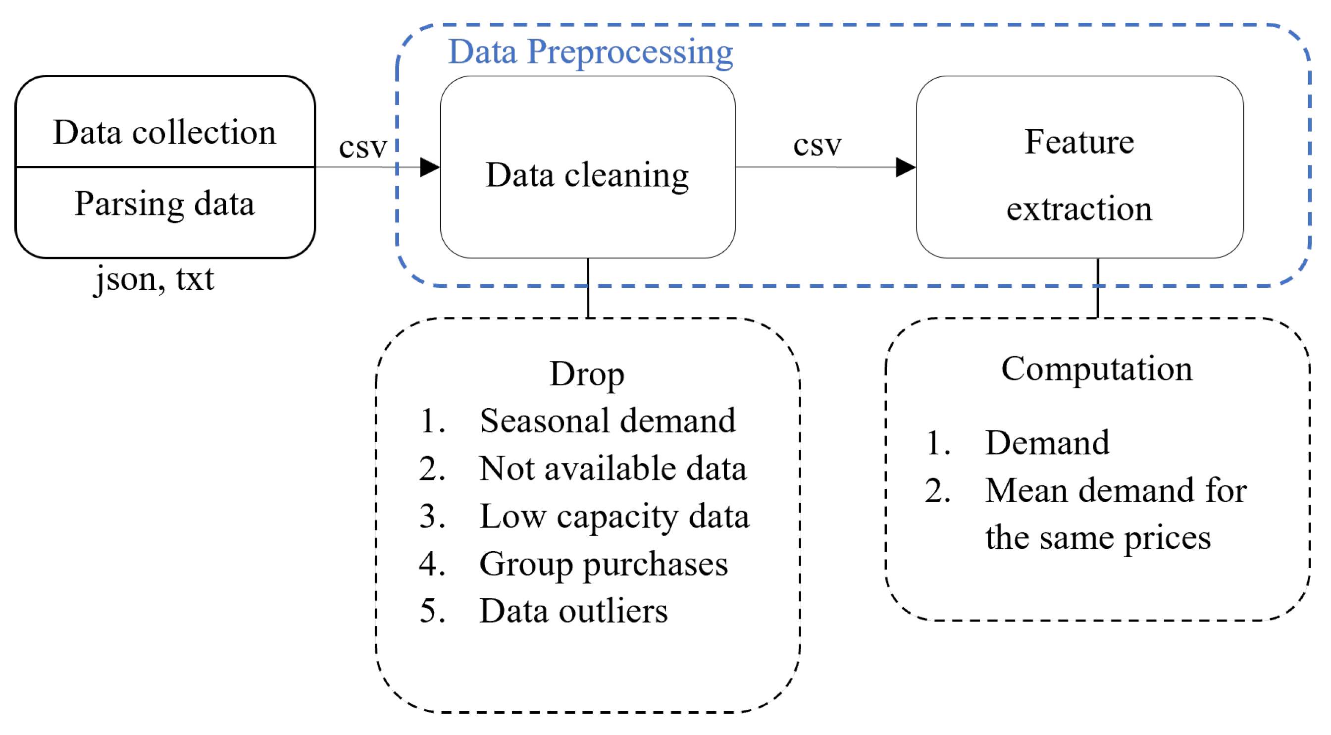
Data pre-processing in the dynamic pricing problem of ticketing systems is divided into two major steps, namely data pre-processing and feature extraction.
At the stage of data pre-processing, it is necessary to analyze the data and identify and remove segments that hinder the implementation of the set goals, namely demand anomalies, for which dynamic pricing is a separate task. One should also delete service records for which there is too little data; for example, as a result of cascading outages of the data collection algorithm. Moreover, one should remove outliers in the data. The used data pre-processing scheme is shown in
Figure 2. The processes shown there are described below in more detail.
Data Cleaning
Deletion of data that form irregular intra-annual demand for holidays.
Deletion of data for which a certain amount of data are missing days before the service:
- a.
Compute the fullness, which is equal to the average number of missing data for each service, service class, and date of service.
- b.
Drop data if fullness is less than or equal to the set threshold.
Deletion of data for which the maximum relative capacity (MRC) is less than the set threshold:
- a.
Compute the MRC, which is equal to the ratio of the maximum capacity for each service, service class, and date of service.
- b.
Drop data if MRC is less than or equal to the set threshold.
Deletion of group ticket purchases:
- a.
Compute the reduced capacity (RdC), which is the ratio of the capacity to the maximum capacity for the entire dataset.
- b.
Compute the mean reduced capacity (MRdC) for all services and service classes.
- c.
Compute the step of MRdC (SMRdC), where SMRdC equals the difference between MRdC and date-shifted maximum absolute MRdC.
- d.
Obtain quantiles of SMRdC, which are designated as , , .
- e.
Compute threshold such as upper inner fence.
- f.
Drop data if MRdC is more than or equal to the threshold.
Removal of other outliers using principal component analysis (PCA):
- a.
Obtain principal component of h.
- b.
Drop data if principal component is less than or equal to the threshold being set.
The set thresholds, according to which outliers are removed, are obtained using graphical analysis.
After receiving the cleaned data, the demand d should be computed. For the convenience of calculating the values of demand for the available capacity values h, a summary table is compiled, the indices of which are the service numbers, days of the week of service, dates, and classes of service. The pivot table columns should contain capacity data h for the days prior to each service.
Feature Extraction
Formation of a pivot table of capacity values by days before the service.
Formation of a pivot table of capacity values shifted by one day.
Computation of consumer demand
(
3).
Formation of a price-averaged demand model.
The resulting pivot table of average demand values is used to model the price elasticity of demand.
4.2.2. Missing Value Restoration
At the initial stage of pre-processing—data cleaning—records corresponding to the dates of train departures on holidays were removed from the dataset. Tickets for trains departing during the holiday time period are observed to have abnormal demand, which adds an irregular intra-annual component to the general type of demand. Thus, the solution of the problem of dynamic pricing in a given period of dates seems to be a special case, which should be considered in a separate study.
The items that were removed were: records corresponding to each train and service class with each departure date for which data were completely missing or more than of demand data was missing in the last 30 days before the train’s departure; each train and class of service whose capacity changed abruptly for each of the departure dates, where such capacity behavior corresponds to the pickup or uncoupling of cars by the transport company after the start of ticket sales and should be considered as a separate task; records corresponding to significant group purchases or ticket sales; other outliers (principal components less than or equal to ).
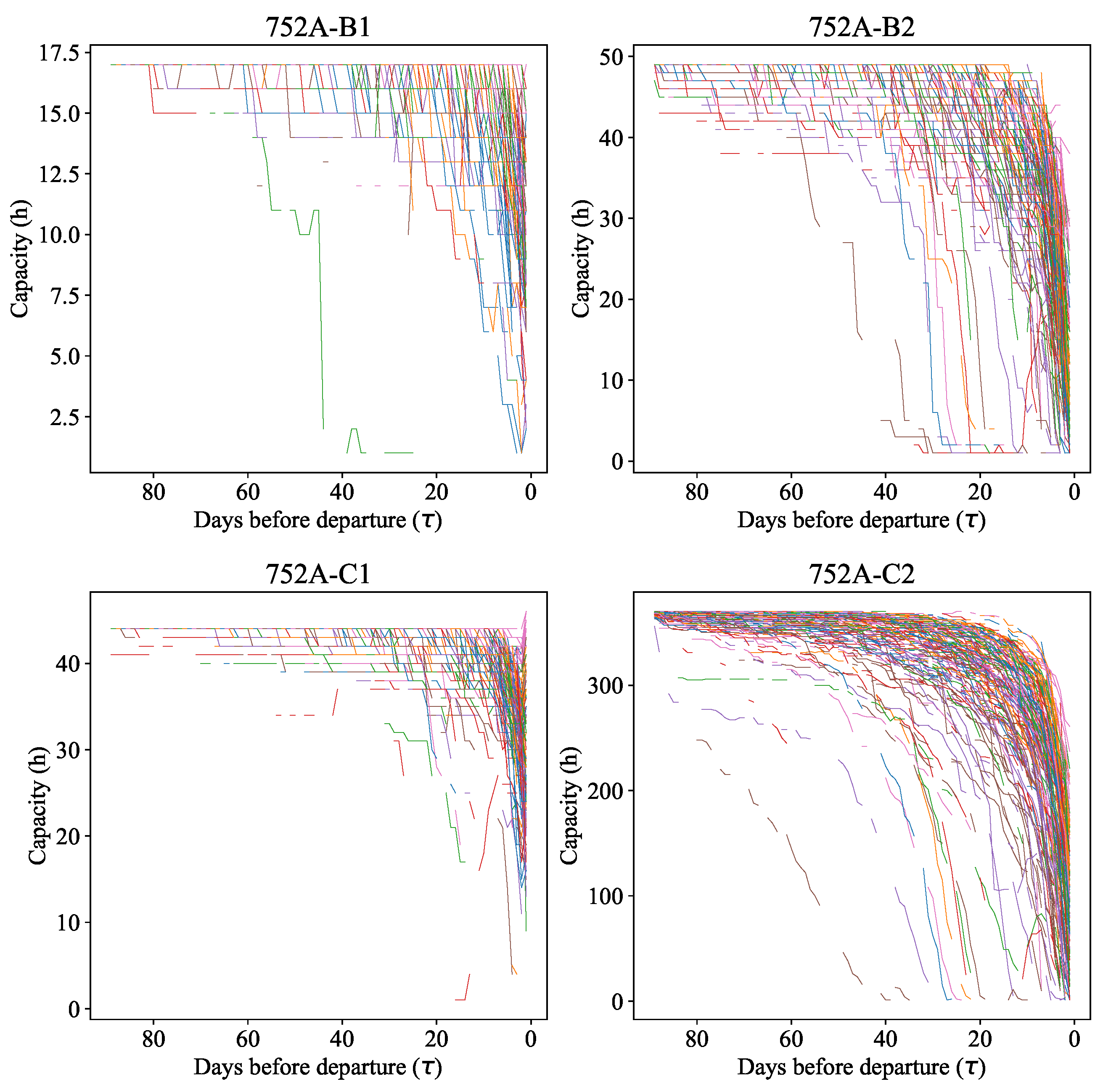
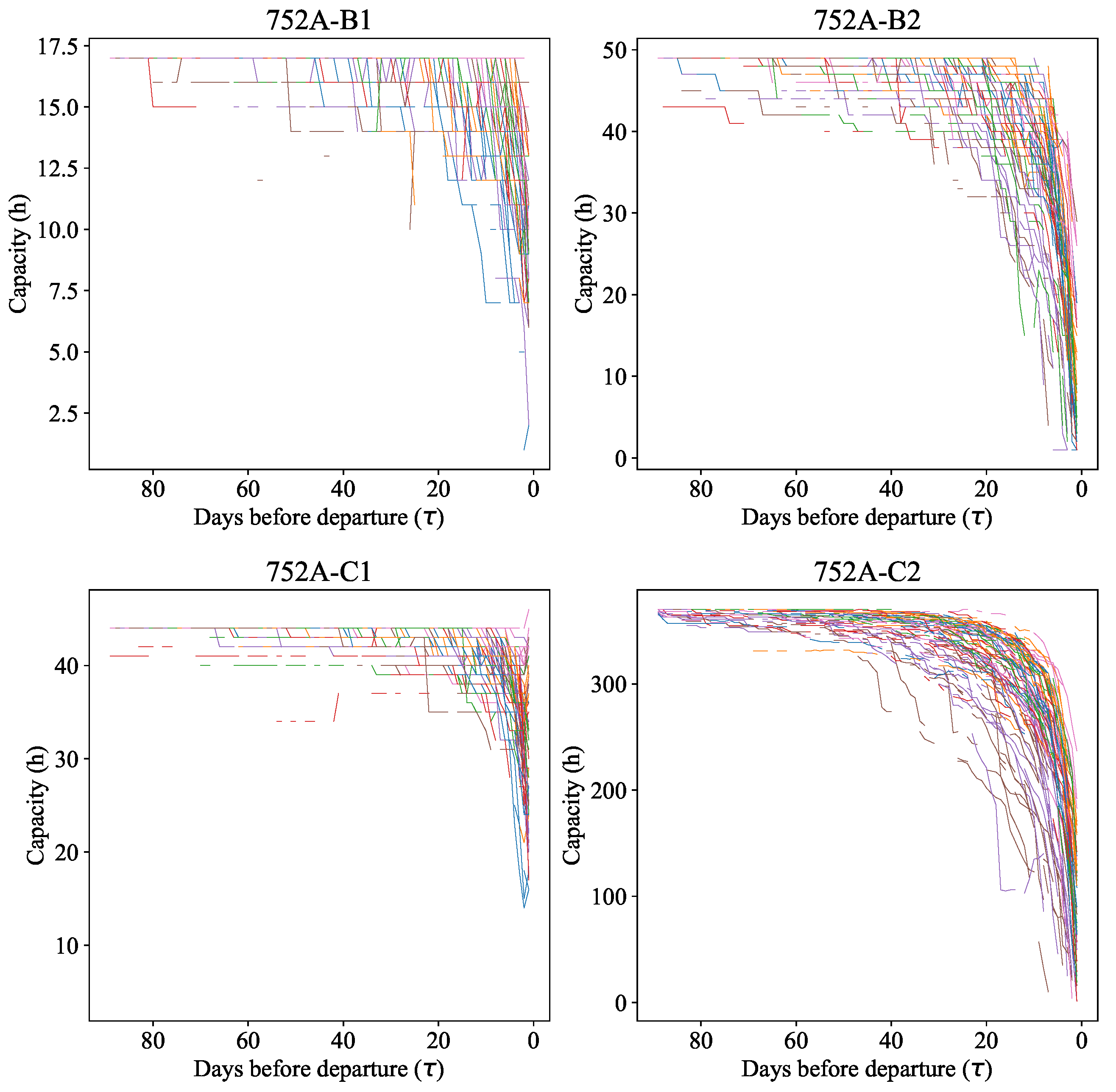
The capacity data received for cleaning and the data obtained as a result of cleaning are shown in
Figure 3 and
Figure 4, respectively.
Figure 3 shows the capacity of the train for all those present in the set of departure dates. The capacity of train cars corresponds to the company’s pricing policy. The popularity of service classes increases with a decrease in the ticket price, so class C2 is the cheapest and B1 is the most expensive.
The capacity characteristic for hooking up new cars to the train is visible on the graph for service class C1—the pink line—when the number of vacant seats increases abruptly when approaching the date of departure of the train. Group purchases are characterized by a sharp, almost linear decrease in the number of vacancies. The irregularity of demand can be seen in the example of service class C2—the brown line—when the number of free seats decreases almost linearly long before the day of train departure; in this case, tickets already run out 40 days before departure.
It should be noted that some phenomena characterizing the hooking of new railway cars to the train still have not been removed; for example, the capacity for class C1 (
Figure 4) is a pink line. Such phenomena should be isolated and removed in a non-automated way.
After obtaining the cleaned capacity values, the demand is computed, the dependence on the price of which is the price elasticity of demand.
4.3. Data Description and Preliminary Analysis
The structure of the data used is summarized in
Table 3. For the experiments described in the paper, the data for the so-called “Sapsan” trains (that depart on different weekdays) that operate between Moscow and St. Petersburg (Russia) are used. They are examples of high-speed intercity trains with a few stops on the way, similar to Beijing–Tianjin intercity trains in China (operated by China Railway High-speed, CRH), Barcelona–Madrid intercity trains Alta Velocidad Española (AVE) operated by Renfe, the Spanish national railway company, etc. Note that each train has four classes of service (we deal with all of them in the multi-class dynamic pricing problem):
B1—First;
B2—Economy+;
C1—Business;
C2—Economy.
Usually, a train consists of 10 vans that can accommodate from 411 to 538 passengers depending on the seat configuration.
Table 4 shows the quartiles of the available place distribution for two classes of service (Business and Economy). Among the “Sapsan” trains, 752A, 759A, 772A, 771A, and 780A were chosen for the experimental study, while the following ones were chosen for illustration in plots in what follows:
Type A: Train number 752A with the route “Moscow—St. Petersburg”, with departure on Friday;
Type B: Train number 780A with the same route, with departure on Thursday,
The total passenger flow for high-speed trains between Moscow and St. Petersburg was approximately 14.5 thousand passengers per day in 2021. There is a strong pendulum mobility and weekly rhythm, with a tourist load returning after COVID-19. While these high-speed trains are an alternative to airplanes, people primarily use them for convenience. The trains are usually very well-filled, sometimes up to 100%, but tickets are often bought in the last few days, particularly for business trips. An additional description of the selected trains is available in
Table 5. Note that the chosen high-speed trains are highly demanded and are indicated as those with dynamic pricing on the railway company’s website.
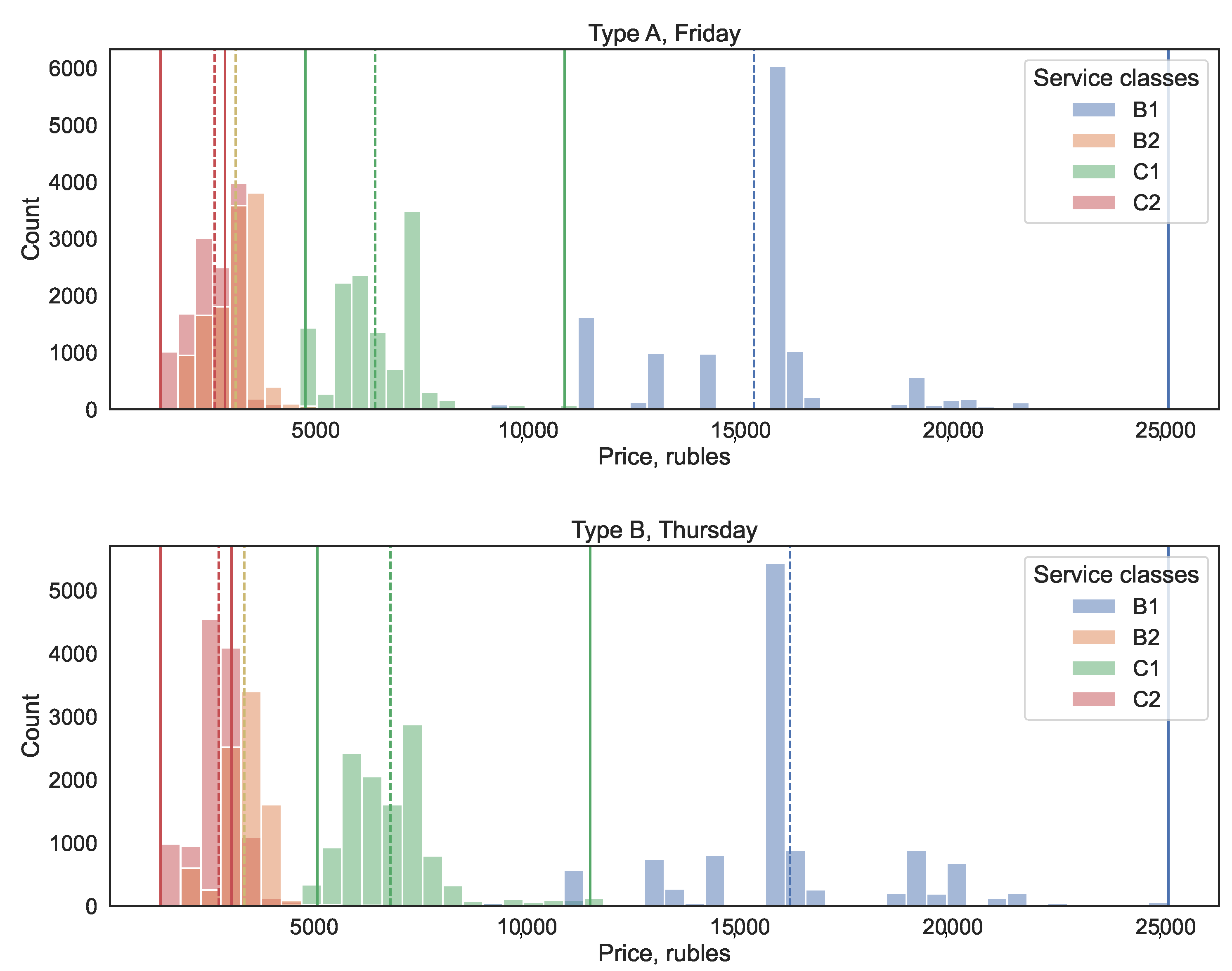
A simple analysis of the data shows the typical price intervals for different classes; see
Figure 5. It should be noted that the proximity of the price ranges of the least expensive classes C2 and B2 is caused by the pricing features of the additional service. Class B2, unlike C2, includes meals. At the same time, the new restrictions do not enter each other’s boundaries, which, in our method, allows us to avoid the multiplication of demand for overlapping classes, where such demand behavior would be uncharacteristic for the company.
Using the data referring to
Figure 5, the price ranges that are natural for the trains in the period under consideration are found. Namely, the average prices by class are calculated, the average of the average prices for these classes is taken for the price border with an existing neighboring class, and the extreme value of the price is taken for the price border for classes without an existing neighboring class. These price ranges are further used as the constraints (
12). In general, other ranges are possible as these would probably make the dynamic pricing process less restrictive.
Furthermore, the dataset of the form (
4) (i.e., the price–demand pairs) is obtained via (
3). These data represent the result of the dynamic pricing process (hidden) in the railway company.
4.4. Surrogate Models and Their Errors Used in Simulation
In what follows, the dynamic pricing problem for 13 days prior to train departure, i.e.,
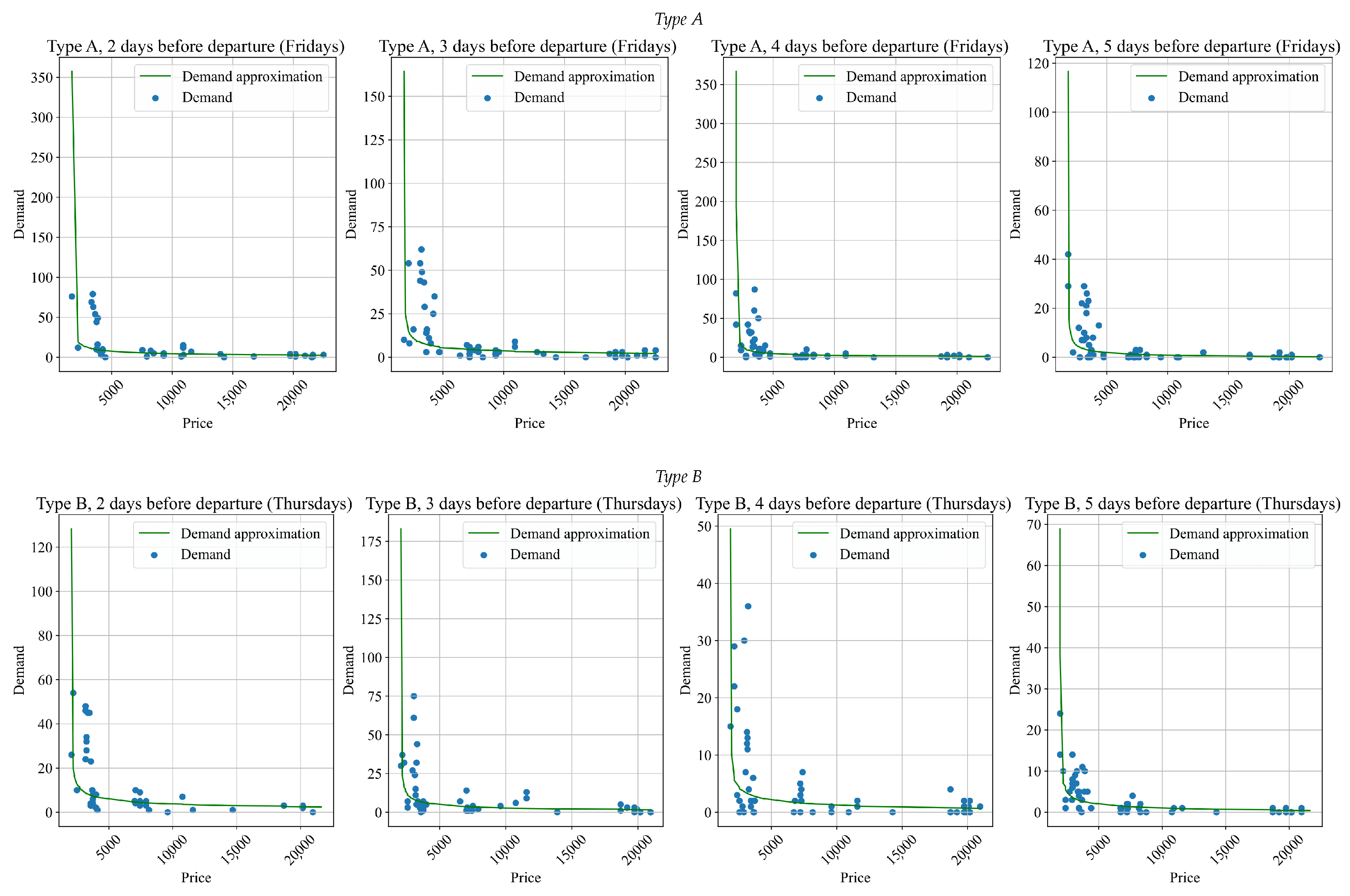
, is considered. The surrogate price elasticity of demand model of the form (
6) for each
for the trains under consideration is then built; see
Figure 6.
Note that the prices and demand in
Figure 6 are for all available classes. It is seen that the demand is rather high for cheap tickets and low for expensive ones (this is expected). Furthermore, the price elasticity of demand is well-described by the power function chosen. One can find the parameters of the resulting surrogate models in
Figure 7.
As seen from
Figure 7, the conditions in (
6) for the
and
coefficients are met, and the price elasticity of demand model describes the dataset received from the hidden model in the expected way. It is important to note how dramatically the coefficients depend on
and may oscillate from day to day.
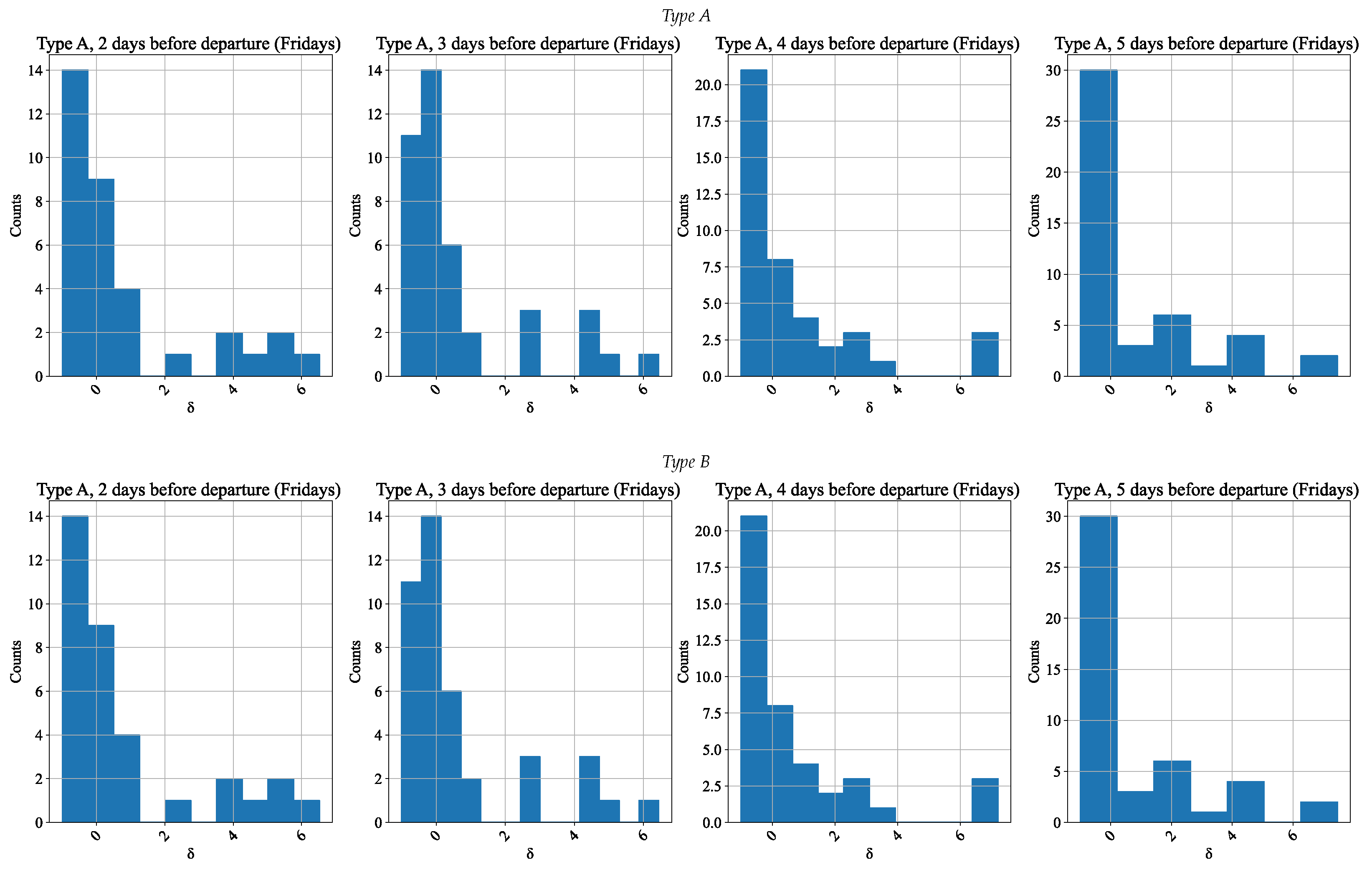
In order to proceed to further simulation, the residuals (errors) of the power function model chosen were analyzed. According to (
6), there is the relative error, which is rather suitable for the power function model.
Figure 8 shows the empirical relative frequency distribution (eRFD) of the errors of the surrogate model.
These errors were further used during the Monte Carlo simulation by (
6) for each
. Such a simulation was performed 100 times and, for each case, the optimization problem (
11) with the constraints (
12) determined by the data above was solved.
4.5. Dynamic Pricing (Optimization)
Once all the necessary components of the objective function (
10) are found, the optimization procedure can start. In order to cope with it, a variant of the differential evolution method (a version due to [
40]) that performs optimization by maintaining a population of candidate solutions and creating new candidate solutions by combining existing ones, and then keeping the candidate solution that has the best score, was used. In particular, the version from Python’s scipy (
https://docs.scipy.org/doc/scipy/reference/generated/scipy.optimize.differential_evolution.html, accessed on 7 May 2023) was used.
An important setting of the method is the population size parameter, which is calculated as the product of the parameter (in scipy) and the number of variables to be optimized, which, in turn, is equal to the product of the number of classes and the number of days before the departure of the train 13, . For experiments, the parameter was chosen to be equal to 1, 5, and 10. As expected, the larger the , the higher the quality of results obtained, on average. However, a large leads to a high computational time. In order to have a trade-off between the quality and time, for illustration in this paper was chosen.
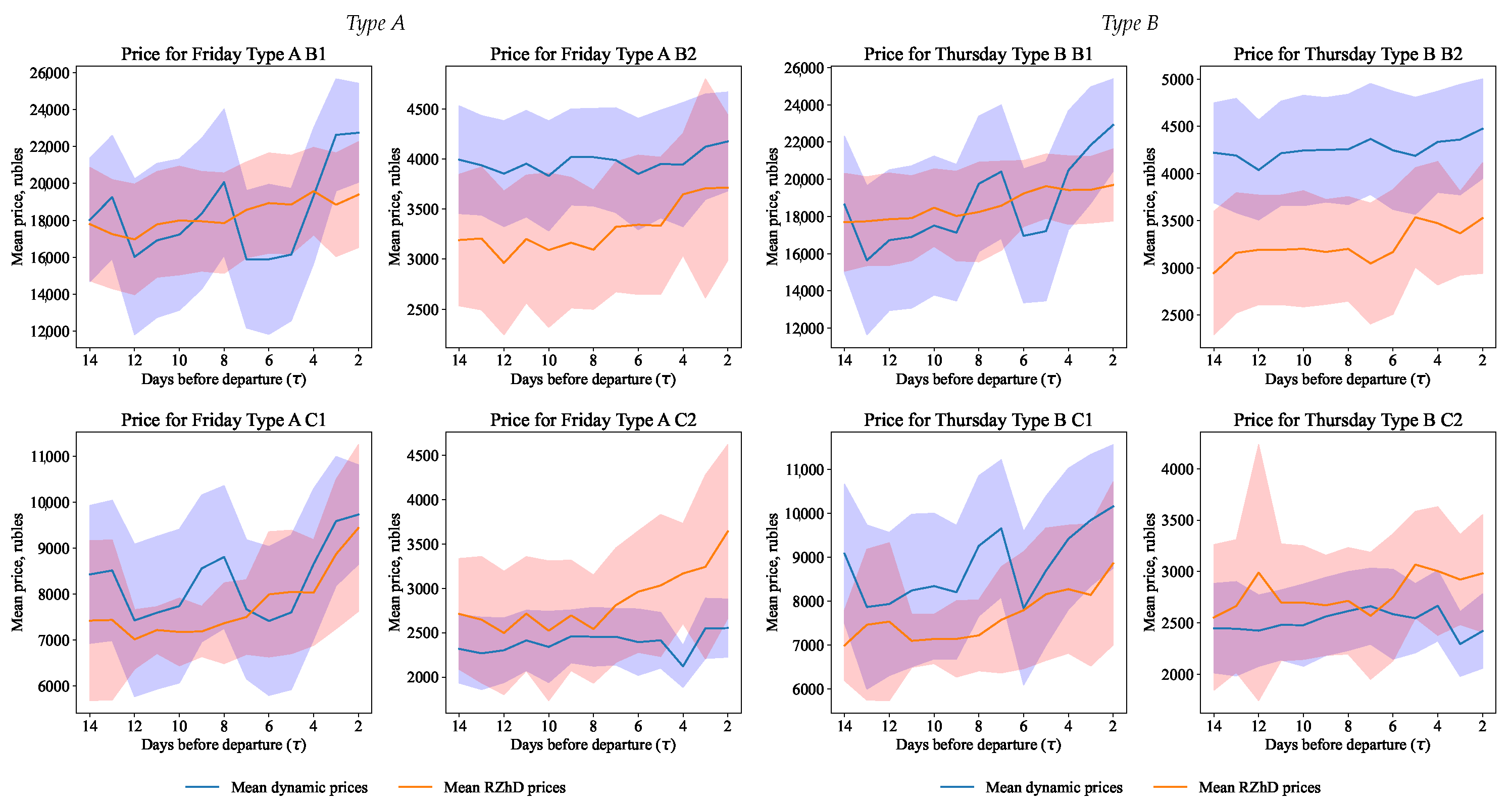
Having received the constraints and tuned the optimizer, the confidence intervals of the form (
15) for prices, demand, and revenue for the Monte Carlo simulation and our dynamic pricing model and the railway company model (hidden to us) were found; see
Figure 9,
Figure 10 and
Figure 11, correspondingly.
Having obtained the values of the prices and demand, it is necessary to calculate the company’s revenue, which can be obtained using this strategy.
Recall that the methodology for calculating the railway company revenue involves an element-by-element multiplication of the data array averaged over demand prices by the corresponding prices; see (
14). After that, the confidence interval for revenue of the form (
15) of revenue for the day before departure for each class separately was determined. The total revenue was calculated as the sum of the average revenue by class for each day before the departure of the train.
Besides the trains of Type A (752A Fri) and Type B (780A Thu), calculations of summarized revenue obtained via simulation and from the real-world railway company data for the trains mentioned at the beginning of
Section 4.3 were made, and the results are shown in
Table 6. In this table, the revenue changes comparable with or more than the standard deviation of both the simulation and railway company data samples are shown in magenta. Using the table, one can rank the dynamic pricing systems for different trains and see the potential for improving the hidden-to-us company’s model.
The average capacity values were used as the upper limit during optimization to monitor the achievement of the limits by the optimizer and the proposed capacity, where the demand for tickets by class is shown in
Table 7.
4.6. Results and Discussion
As was stated earlier, the effectiveness of the proposed method was tested on the dataset collected from the website of Russian railway passenger carrier company for the period from 12 April 2021 to 17 March 2022. In this paper, experiments on 11 diverse trains from Moscow to St. Petersburg are presented as an example. It can be concluded that the resulting pricing (
Figure 9) strategy relies to a greater extent on the cheapest service class (C2), as can be seen from the price given by the optimizer for this class of service, while the average optimal price for more expensive classes (B1, B2, C1) of service is above the average optimal price of the railway company. This optimization approach is consistent with the expectation of the company, which sets this trend by setting the largest number of tickets for the class from which the company expects to receive the maximum revenue.
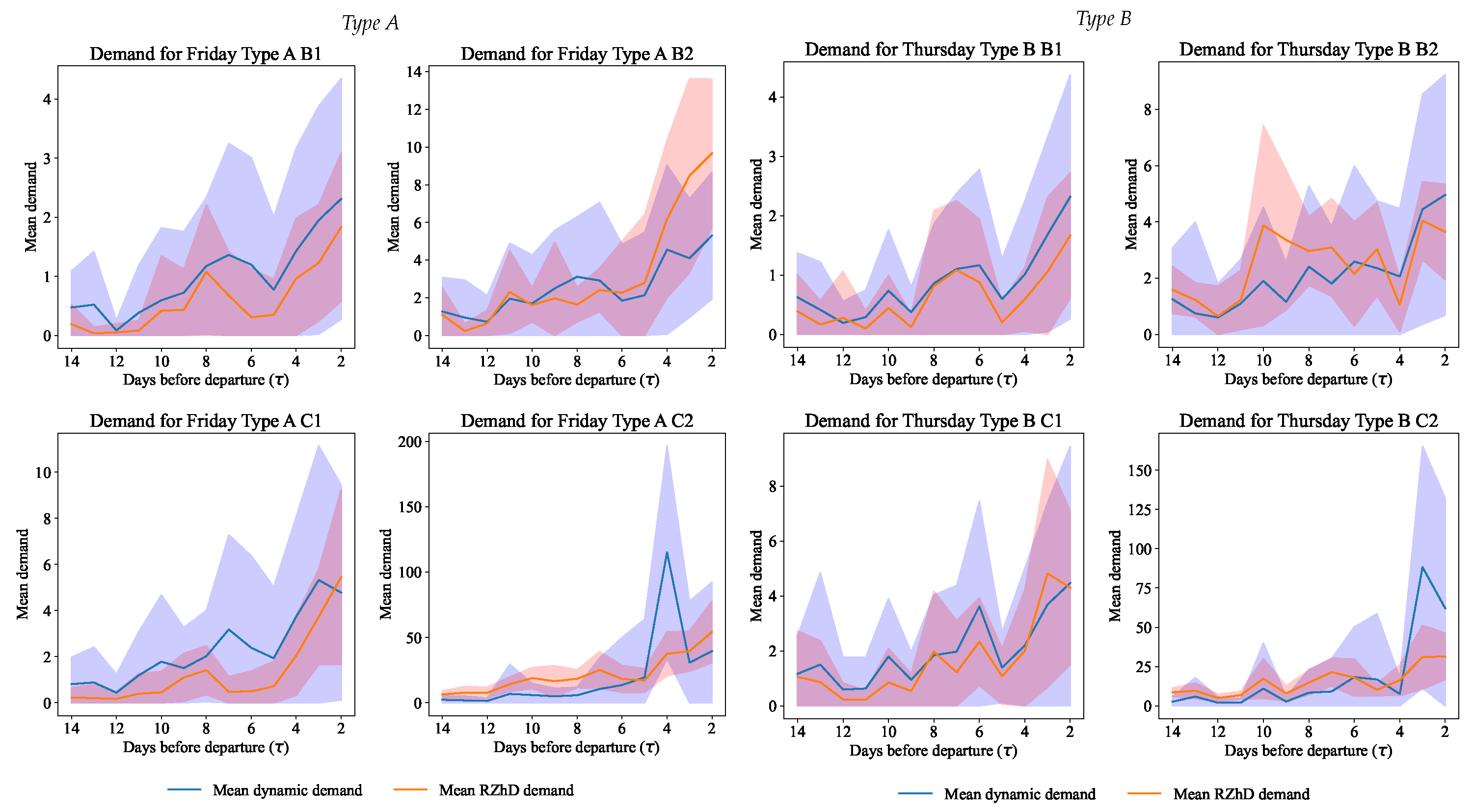
According to the received new pricing strategy, the demand (
Figure 10) can be observed. The optimization suggested an increased demand in the last few days before the departure of the train for the most popular class of service, which is achieved by corresponding prices. In accordance with the available description of the price elasticity of demand, for the most expensive classes of service, this effect is less noticeable due to the flatness of the function when the price increases. This effect corresponds to the expected one, where the demand for the most expensive train classes is historically not large, which is also expressed by the company’s policy on the initial formation of the number of seats by class of service.
As can be seen from
Table 6, the quality of dynamic pricing of the
Type A and
B trains are rather similar in the simulation and in the real-world railway company data, taking into account the deviation calculated. In a sense, this means that the dynamic pricing system of the railway company works similar to the simple model proposed by us and gives the highest-quality ranked results among the other trains considered. At the same time, the results for other trains are more interesting and show that the existing system has a high potential for improvement (especially since it is compared with the simple data-driven model that we built). Again considering the deviation, the quality performance difference (in terms of the company’s revenue from ticket sales) between the hidden and exposed models varies here up to 57% on average, which is rather impressive. In other words, the results show that, depending on the train type, the quality performance difference (in terms of the company’s revenue from ticket sales) between the hidden and exposed models can vary by up to several dozen percent on average, indicating the potential for improvement in the company’s existing (hidden to us) dynamic pricing model.
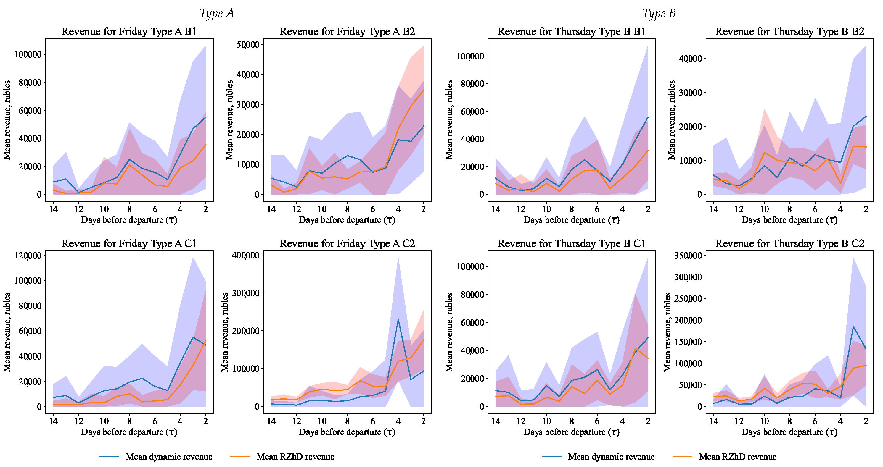
As expected from the obtained values of demand and prices, the company’s optimized revenue largely depends on the pricing policy for the most popular and, accordingly, the cheapest service class (see
Table 7). This revenue optimization is in line with the overall revenue generation strategy of the passenger rail company, whose historical data show that the company always expects to generate the bulk of revenue from the most desirable class of service.
At the same time, this strategy of multi-class optimization allows one to receive increased revenue, including from classes of service that are not the main ones in terms of revenue. This indicates that the railway company’s hidden model is somewhat inferior to the dynamic pricing based on the surrogate model. At the same time, it should be noted that the company’s model is most likely based on a predictive price elasticity of demand model, whereas, in this paper, the actual values of demand are used. The lower income of the hidden model may be due to the prediction error. Nevertheless, the method proposed in this study make the quality ranking of the dynamic pricing models rather evident and similar to what we would have after testing the hidden model in reality.
It should be noted that the dynamic pricing method used and the demand model itself are simplified, for example, in comparison with methods based on deep learning. In addition, the presented model works under conditions of unknown actual price limits for service classes existing in the company. Moreover, the data used in our study were cleared of holiday demand anomalies, thus possibly “losing” the corresponding part of demand within the Monte Carlo simulation. It is interesting that, even in the simplified setting, we have the data-driven dynamic pricing model that shows a better performance than the existing company’s model.
5. Conclusions
Motivated by the lack of reproducibility in the field of dynamic pricing for train ticket data, this paper proposes a simple, data-driven method called DPRank with open-source code and publicly available data. The method allows for the evaluation and ranking of the quality of existing dynamic pricing models using only open data from online ticket systems. Specifically, it builds a surrogate price elasticity of demand model using public data generated by the hidden dynamic pricing model, and then applies the surrogate model to build the exposed model of dynamic pricing. The hidden and exposed models were further compared in terms of revenue optimization quality through a Monte Carlo simulation method.
The developed method demonstrates the possibility of restoring the pricing model based on open data. Its practical significance lies in its ability to solve various tasks for different actors of the smart urban environment. For carrier companies, it can be used to optimize their pricing programs and increase market volumes in a competitive environment, where pricing programs consider the restored models of other carriers. City or regional government authorities can use this method to optimize the transport system and increase transport accessibility for the population through a flexible coordinating policy of carriers. This includes implementing multitransport routes with convenient connections, single tickets for different types of transport, and dynamic tickets such as a “weekend ticket”. Additionally, this method can serve as the basis of work for transport aggregators in the B2C segment, allowing them to recommend the most favorable offers on routes and prices at a selected time, especially in pre-order or “waiting list” modes. In general, this method will make the mobility of the population more interpretable, which is essential when managing a smart city or region.
The limitation of this method is that it models the potential demand for transportation (which, under certain conditions, can be realized in the form of ticket purchases) rather than the actual use of transportation. Therefore, for managing the mobility of the population, the developed method is not enough, and additional mechanisms are required to contribute to the realization of potential demand, such as popularization and advertising.
In this study, a highly versatile method (implemented on the specified GitHub) was developed that, together with an open data crawling framework for ticket prices, can be used for any railway passenger carrier company. Its functionality was confirmed using the Moscow to St. Petersburg route as an example. However, its effectiveness may vary depending on the specific route’s mode and load, and it may differ between different countries and routes. This fact requires a separate study, which is planned as a part of our future work.

 ,
, 


