


A Review of Wireless Positioning Techniques and Technologies: From Smart Sensors to 6G

Abstract
:1. Introduction
1.1. Contributions
- A comprehensive taxonomy of the related literature in wireless positioning systems over the last 30 years classified according to (i) the localization technique and (ii) the wireless technology employed.
- All the different localization methods and wireless technologies explained from first principles, in order to serve as a self-contained source for the interested audience and facilitate the comparison between the different methods.
- A critical analysis of the different techniques and technologies, identifying existing gaps and challenges and recommending research directions for building the positioning systems of the future.
1.2. Related Studies

| Signal Estimations | Localization Techniques | Wireless Technologies | |||||||||||||||||||||
|---|---|---|---|---|---|---|---|---|---|---|---|---|---|---|---|---|---|---|---|---|---|---|---|
| Ref. | Time-based | Angle-Based | RSS | CSI | Lateration | Angulation | Range-free | Fingerprinting | Environment | GNSS-Indoor | Cellular-Based | FM | LoRa | Wi-Fi | ZigBee | Bluetooth | UWB | Geomagnetism | Acoustic | VLC | RFID | IMU | IR |
| [2] | ✓ | ✓ | ✓ | ✓ | I | ✓ | ✓ | ✓ | ✓ | ✓ | ✓ | ✓ | ✓ | ✓ | |||||||||
| [20] | ✓ | ✓ | ✓ | ✓ | ✓ | ✓ | I/O | ✓ | ✓ | ✓ | ✓ | ✓ | ✓ | ✓ | ✓ | ||||||||
| [17] | ✓ | I/O | ✓ | ✓ | ✓ | ✓ | ✓ | ||||||||||||||||
| [6] | ✓ | ✓ | ✓ | ✓ | ✓ | I | ✓ | ✓ | ✓ | ✓ | ✓ | ✓ | ✓ | ✓ | |||||||||
| [8] | ✓ | ✓ | ✓ | I | ✓ | ||||||||||||||||||
| [9] | ✓ | ✓ | I/O | ✓ | ✓ | ||||||||||||||||||
| [10] | I | ✓ | ✓ | ✓ | ✓ | ✓ | |||||||||||||||||
| [12] | ✓ | I | ✓ | ||||||||||||||||||||
| [13] | ✓ | ✓ | I | ||||||||||||||||||||
| [14] | ✓ | ✓ | ✓ | ||||||||||||||||||||
| [15] | ✓ | ✓ | ✓ | I | ✓ | ||||||||||||||||||
| [4] | ✓ | ✓ | ✓ | ✓ | ✓ | I | ✓ | ✓ | ✓ | ✓ | ✓ | ✓ | ✓ | ✓ | ✓ | ✓ | |||||||
| [5] | ✓ | ✓ | ✓ | ✓ | I | ||||||||||||||||||
| [7] | ✓ | ||||||||||||||||||||||
| [21] | ✓ | ✓ | ✓ | ✓ | I | ✓ | ✓ | ✓ | ✓ | ✓ | ✓ | ✓ | |||||||||||
| [18] | ✓ | ✓ | ✓ | ✓ | |||||||||||||||||||
| [16] | ✓ | I | |||||||||||||||||||||
| [19] | ✓ | ✓ | I | ✓ | |||||||||||||||||||
| [22] | ✓ | ✓ | ✓ | ✓ | I | ✓ | |||||||||||||||||
| [23] | ✓ | I | ✓ | ||||||||||||||||||||
| [24] | ✓ | ✓ | ✓ | ✓ | I/O | ✓ | |||||||||||||||||
| [25] | ✓ | I/O | ✓ | ||||||||||||||||||||
| [26] | ✓ | ✓ | ✓ | I | ✓ | ✓ | |||||||||||||||||
| [27] | ✓ | ✓ | ✓ | ✓ | ✓ | ✓ | ✓ | ✓ | I | ✓ | ✓ | ✓ | ✓ | ✓ | |||||||||
| [28] | I/O | ✓ | |||||||||||||||||||||
| [29] | ✓ | ✓ | ✓ | ✓ | I/O | ✓ | ✓ | ✓ | ✓ | ✓ | ✓ | ✓ | |||||||||||
1.3. Overview
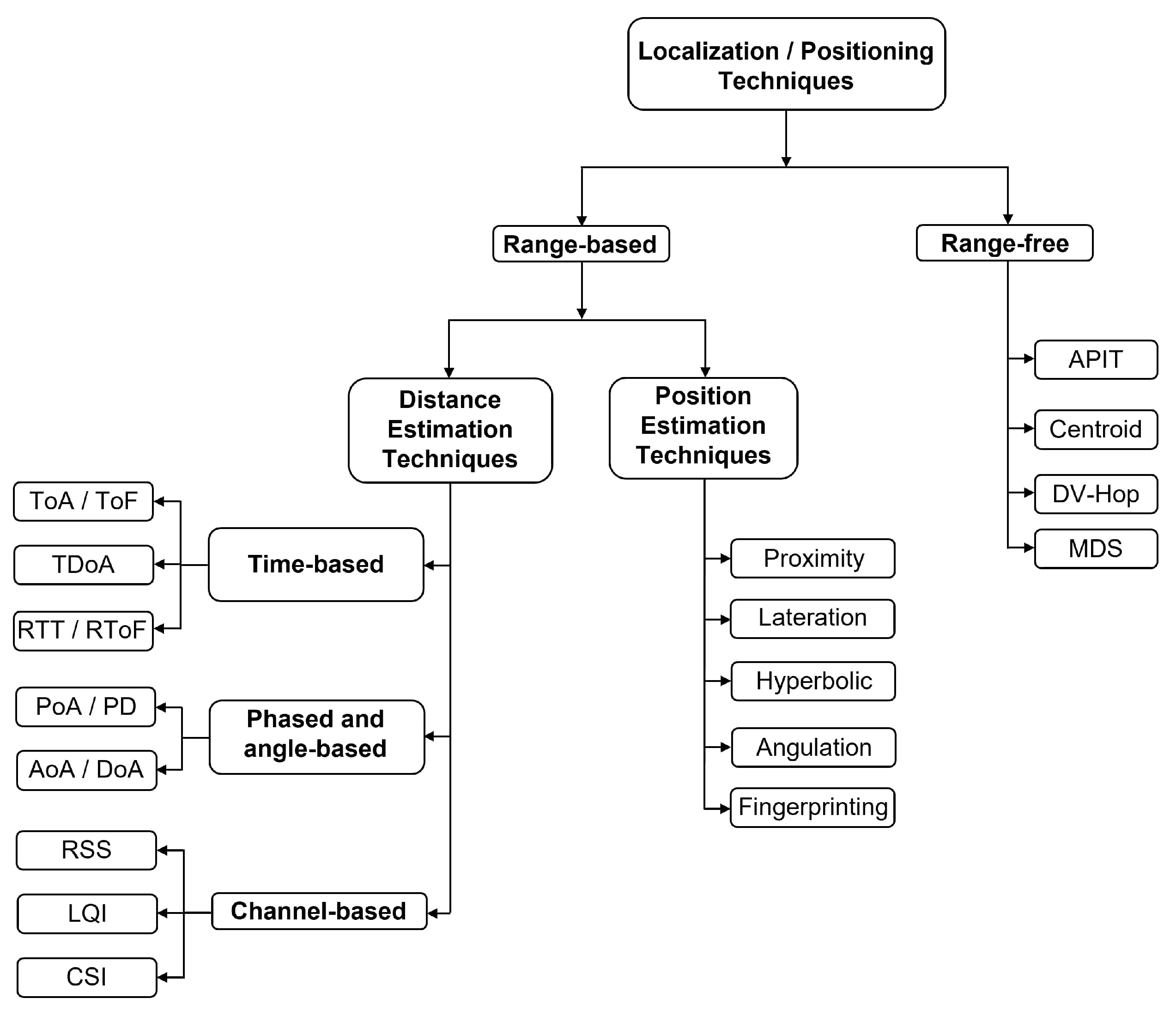
2. Localization Techniques
2.1. Signal Measurements
2.1.1. Time-Based Measurements
Time of Arrival (ToA)
Time Difference of Arrival (TDoA)
Round Trip Time (RTT)
2.1.2. Angle-Based Measurements
Phase Difference of Arrival (PDoA)
Angle of Arrival (AoA)
2.1.3. Channel-Based Measurements
Link Quality Indicator (LQI)
Received Signal Strength (RSS)
Channel State Information (CSI)
| Distance Estimation Techniques | Features | Limitations |
|---|---|---|
| Time of Arrival (ToA) | - More accurate results compared to the RSSI measurements | Precise time synchronization between nodes is required - Highly biased from the environment - Additional hardware may be required |
| Time Difference of Arrival (TDoA) | - Contrary to ToA, TDoA only requires precise time synchronization between the transmitting nodes - It can also be utilized with nodes equipped with speakers and microphones - Provides higher accuracy than ToA - It can be used with different communication technologies, i.e., ultrasound and RF | - Time synchronization between transmitting nodes is required - Performance is degraded in the NLoS signal propagation - Microphones and speakers require LoS and free of echoes conditions for higher accuracy |
| Round Trip Time (RTT) | - It eliminates the need of utilizing different clocks and time synchronization | - It requires bidirectional communication capabilities - Its accuracy is biased from the different changes in the environment - Latencies may occur for fast moving devices |
| Phase of Arrival (PoA) | - It can be combined with other measurements for higher accuracy | - The phase cannot be distinguished, so it can only determine in which fraction of the wavelength a signal is received - It requires LoS |
| Angle of Arrival (AoA) | - At least two transmitting nodes are required - No time synchronization between the nodes is required | - It requires LoS signal propagation - Signals can easily change direction, so accuracy degradation occurs - Its accuracy is proportional to the nodes’ density - Additional hardware is required (e.g., antenna arrays) - Expensive computational cost |
| Received Signal Strength (RSS) | - One of the simplest and most widely used metrics - Supported by most transceivers - Easily scaled to larger areas and multiple users - Minimum infrastructure required - Cost-effective computation | - Its accuracy is affected by the existence of obstacles and multipath propagation - Affected by NLoS - Affected by weather conditions, such as rain [42] - Less accurate than time-based estimations |
| Link Quality Indicator (LQI) | - Contrary to RSS, LQI is included in all received packets | - Only available for ZigBee technology |
| Channel State Information (CSI) | - It can be used as a unique fingerprint - More accurate estimates, compared to the RSS estimations | - It can only be used with technologies supporting OFDM - Special hardware is required (increased cost and complexity) - It is affected by the dynamic changes of the transmitting nodes’ power |
2.2. Range-Based Localization Techniques
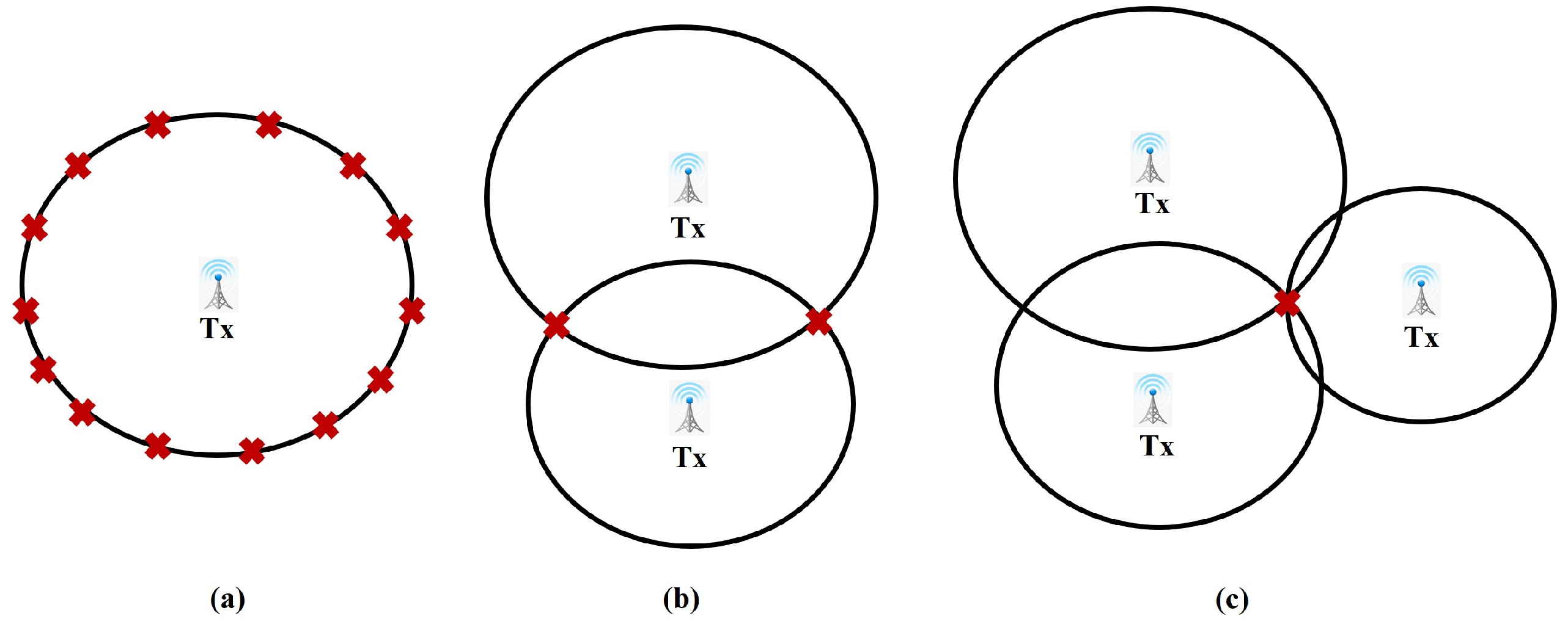
2.2.1. Lateration
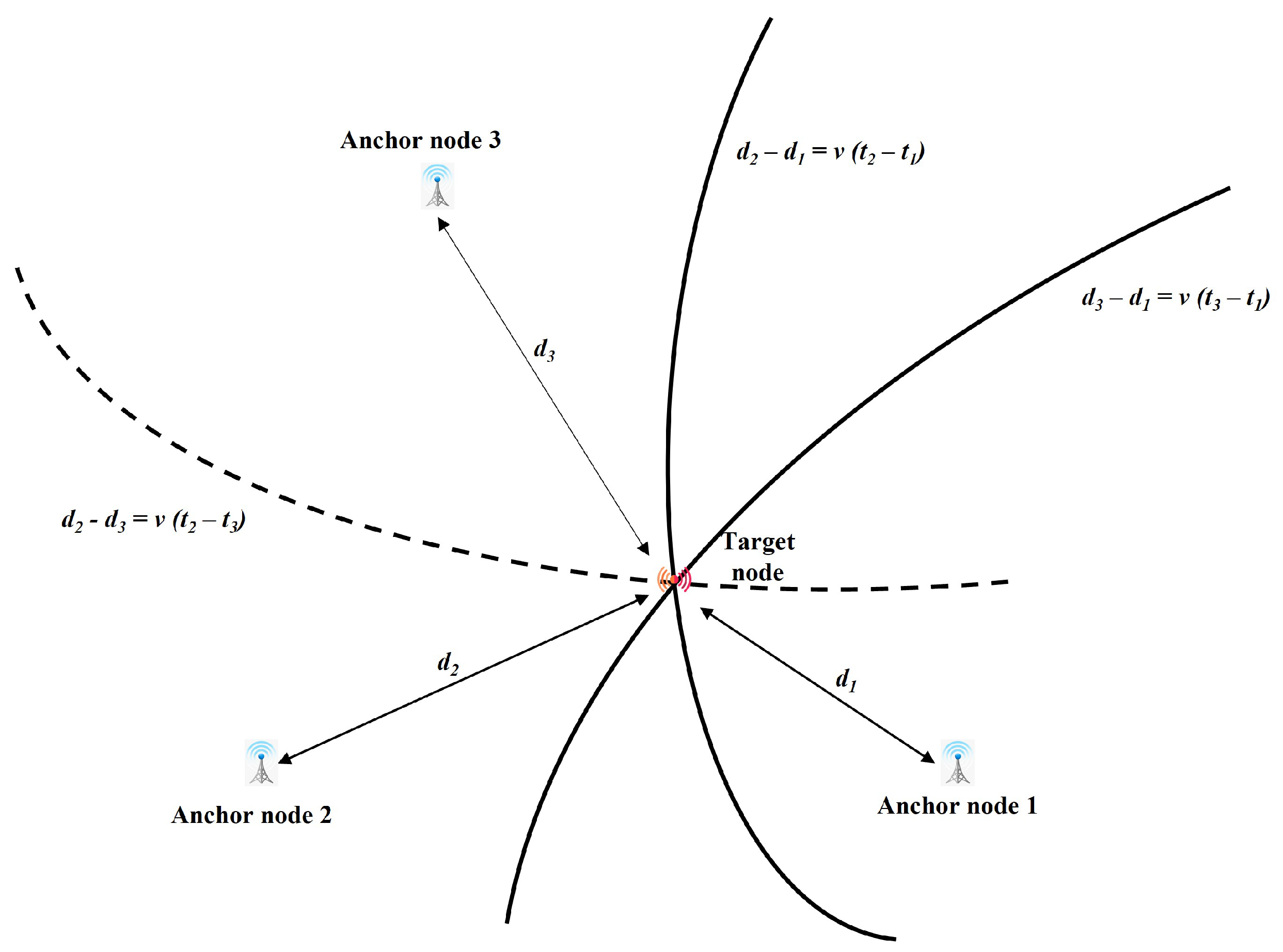
2.2.2. Hyperbolic
2.2.3. Angulation
2.2.4. Multidimensional Scaling (MDS)
2.3. Range-Free Localization Techniques
2.3.1. Proximity Detection
2.3.2. Centroid
2.3.3. Distance Vector (DV)-Hop
2.3.4. Approximate Point in Triangulation (APIT)
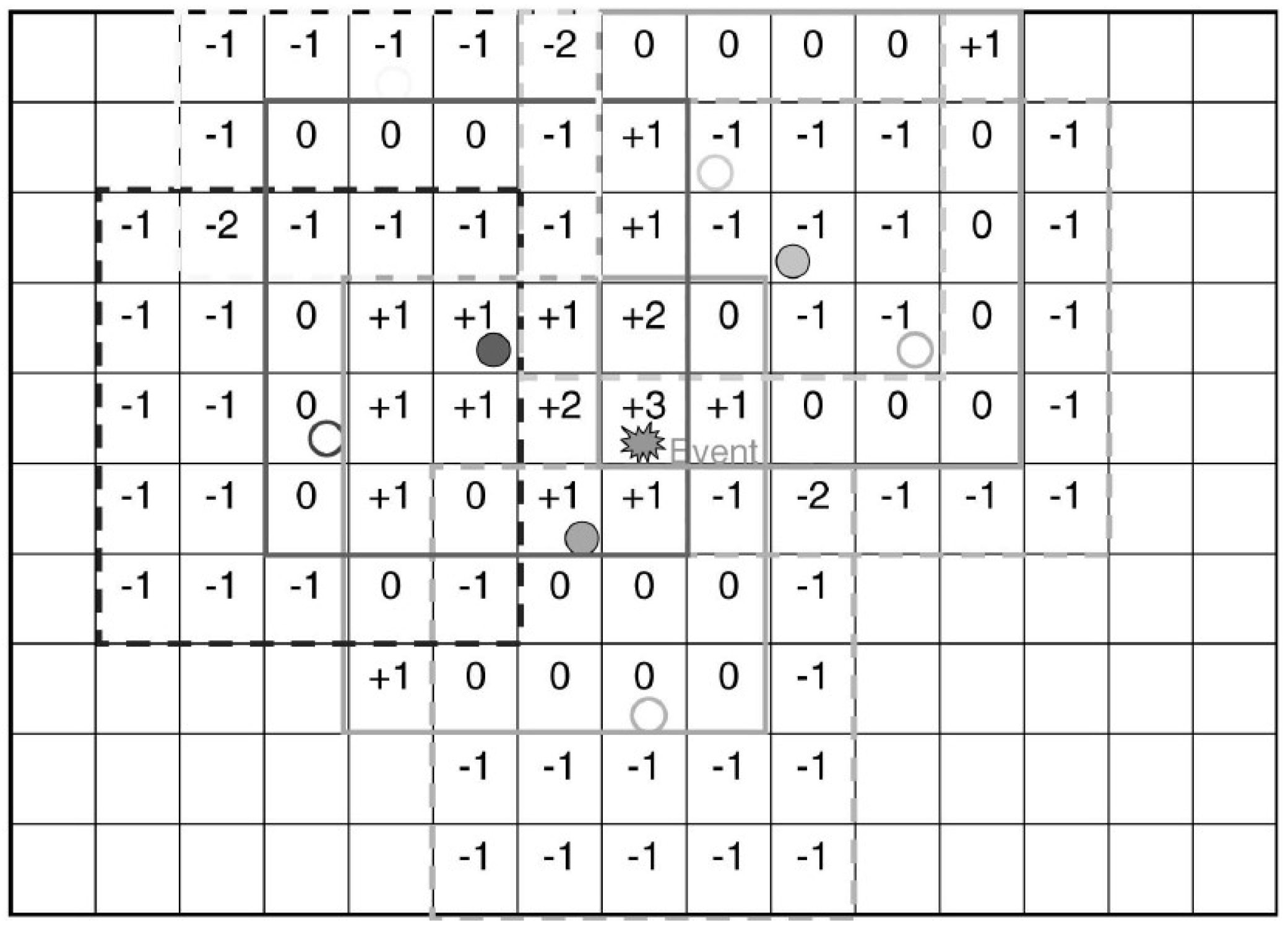
2.3.5. Subtract on Negative Add on Positive (SNAP)
2.4. Machine Learning (ML) Localization Algorithms
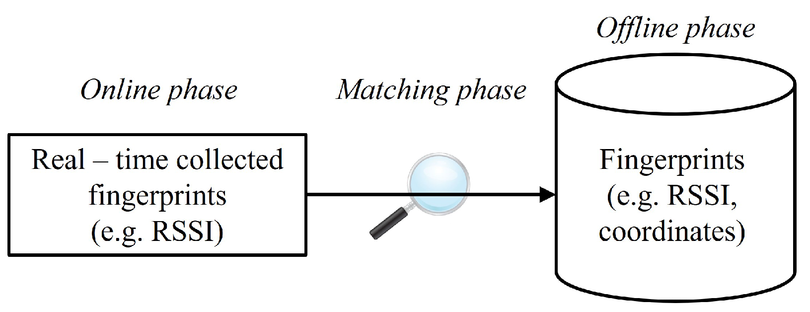
Fingerprinting
2.5. Tracking Techniques
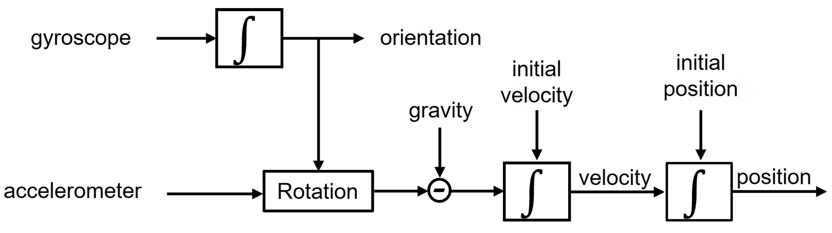
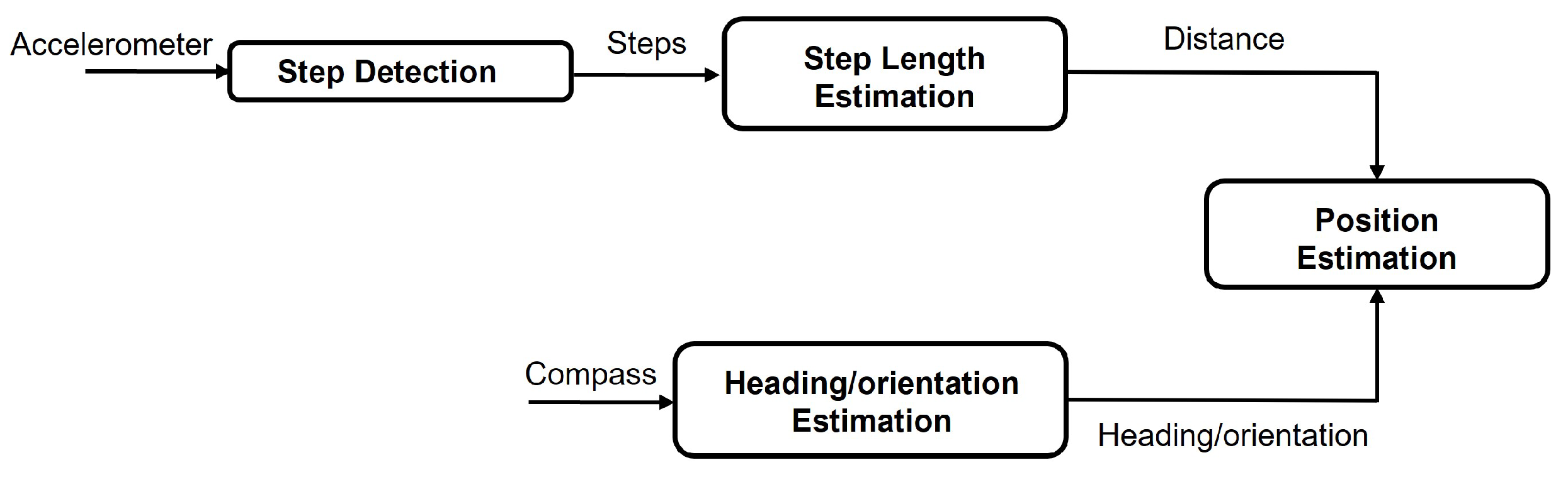
2.5.1. Dead Reckoning (DR)
2.5.2. Filters
2.5.3. Simultaneous Localization and Mapping (SLAM) Algorithm
3. Wireless Technologies
3.1. Global Navigation Satellite System (GNSS)
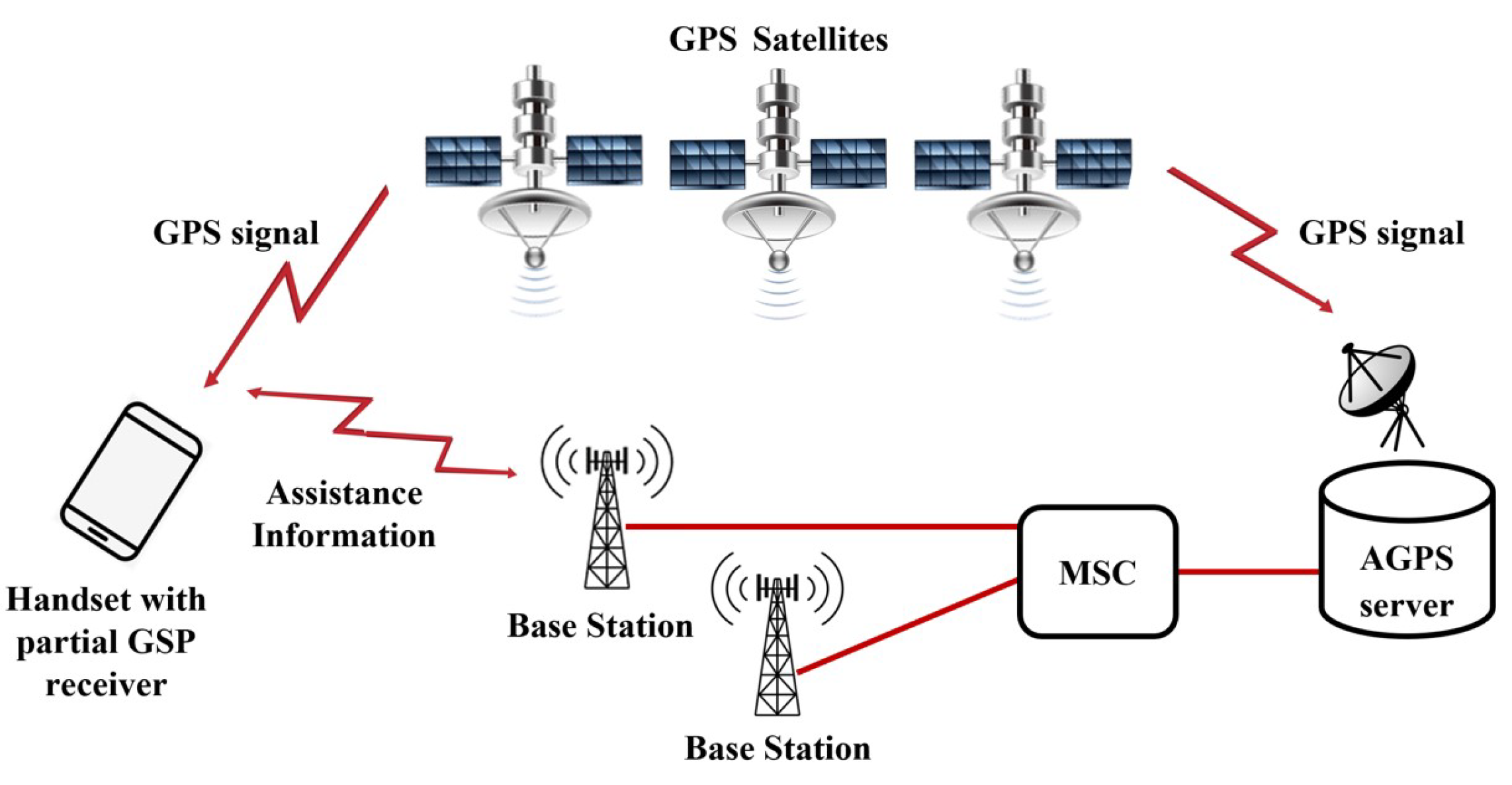
3.1.1. Assisted Global Positioning System (AGPS)
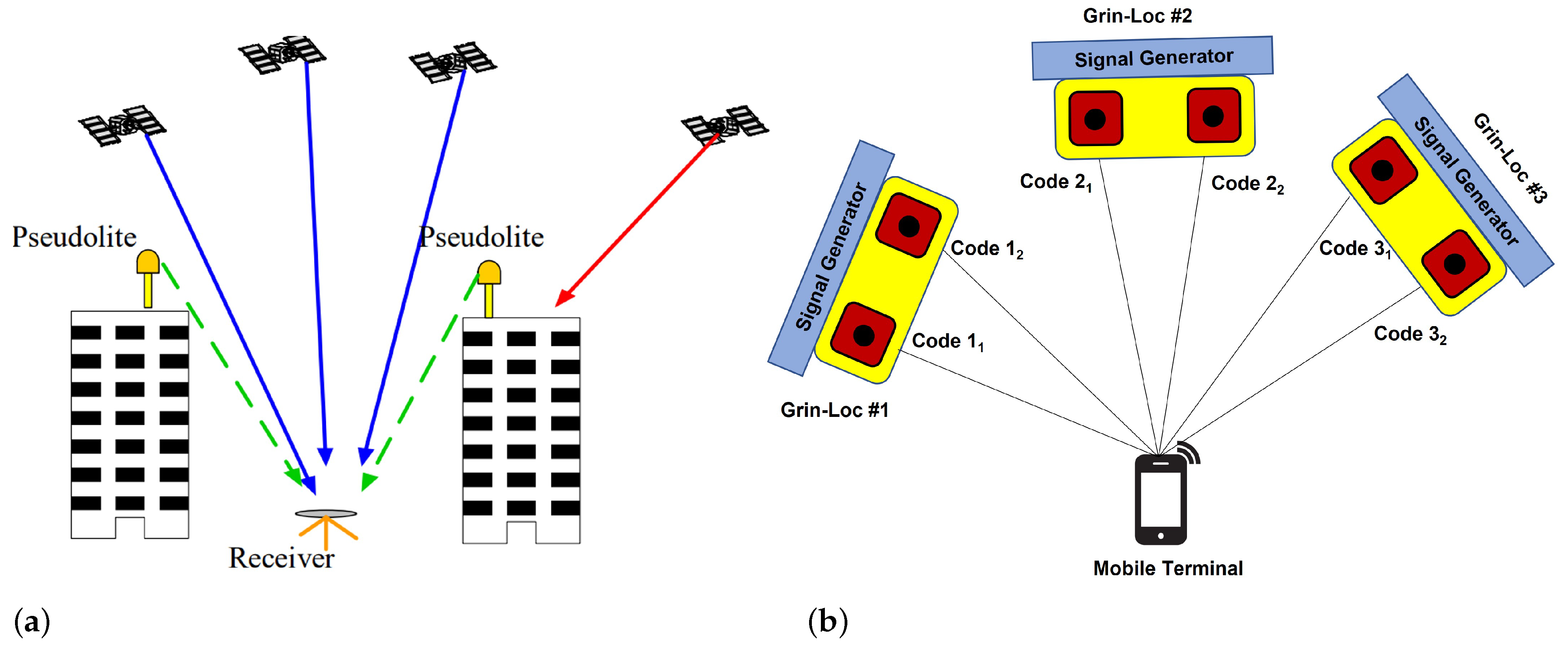
3.1.2. Indoor GNSS Satellites
3.2. Cellular
3.2.1. Global System for Mobile (GSM) Communications
3.2.2. Narrowband-Internet of Things (NB-IoT)
3.2.3. Fifth Generation (5G)
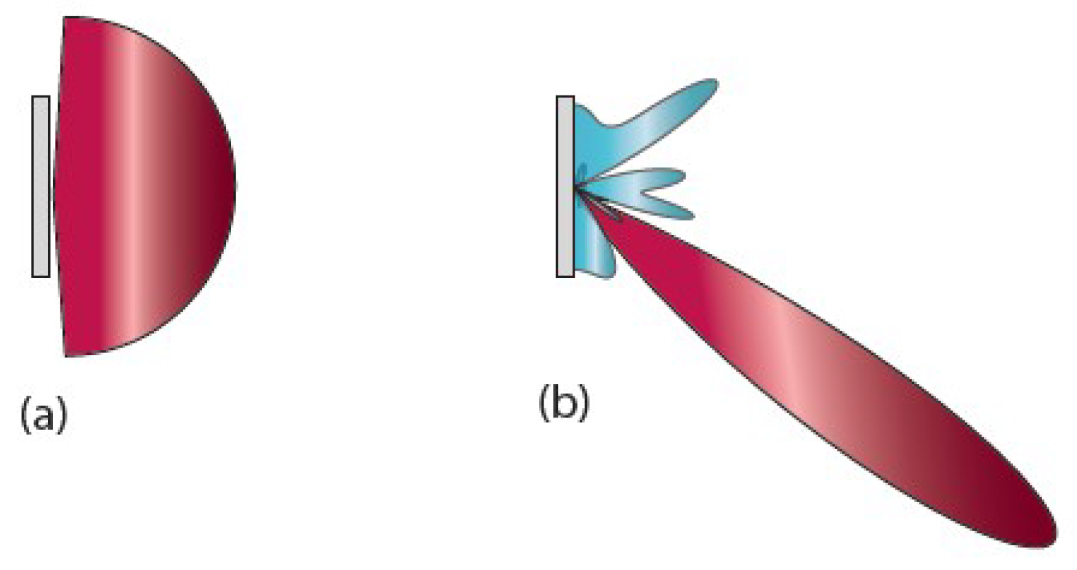
3.2.4. Intelligent Reflecting Surface (IRS)
3.3. Radio Detection and Ranging (RADAR)
3.4. Frequency Modulation (FM)
3.5. Long Range (LoRa)
3.6. SigFox
3.7. Wireless Fidelity (Wi-Fi)
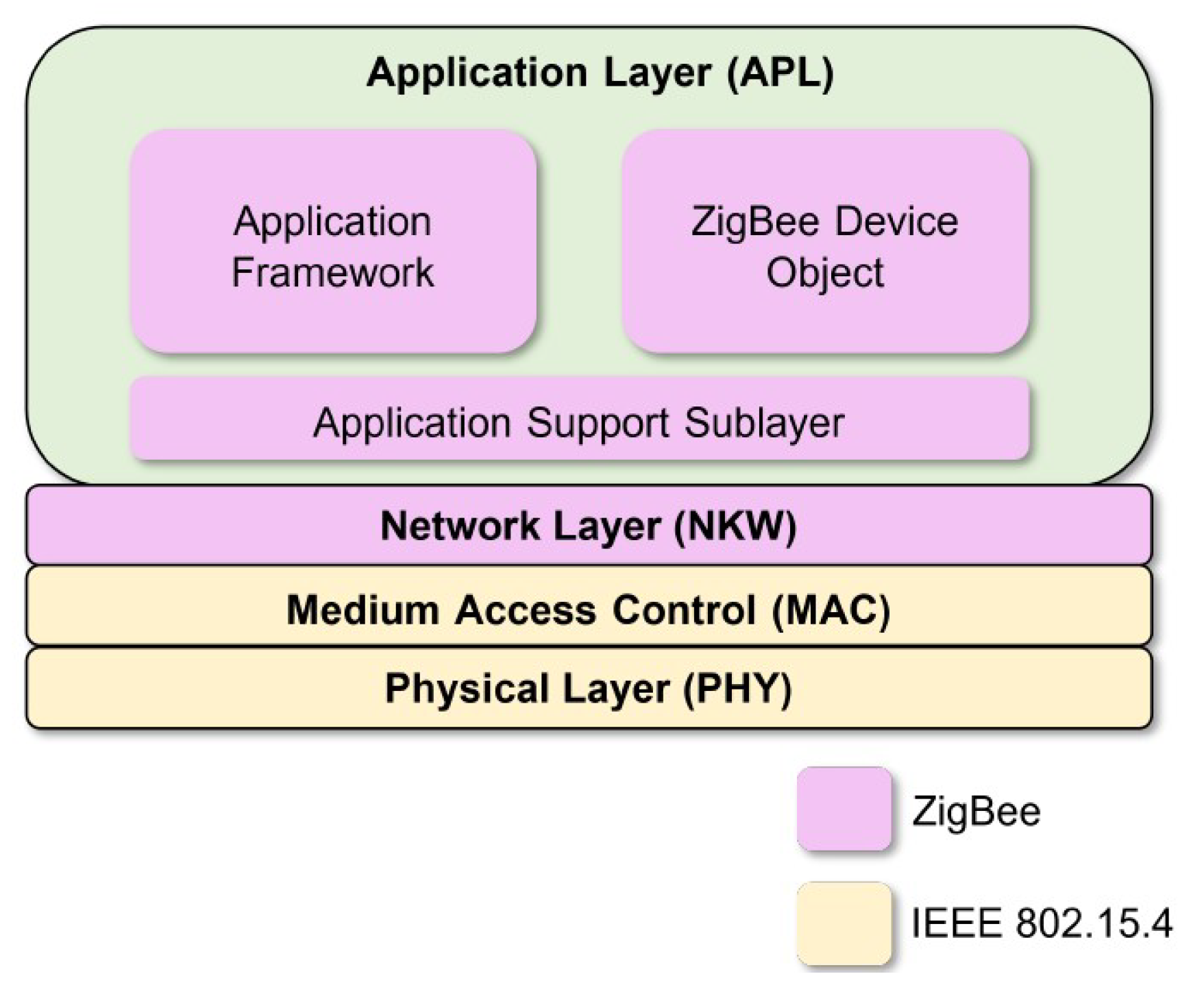
3.8. ZigBee
3.9. Bluetooth
3.10. Ultrawide Band (UWB) Technology
3.11. Geomagnetism
3.12. Vision Positioning Systems (VPS)
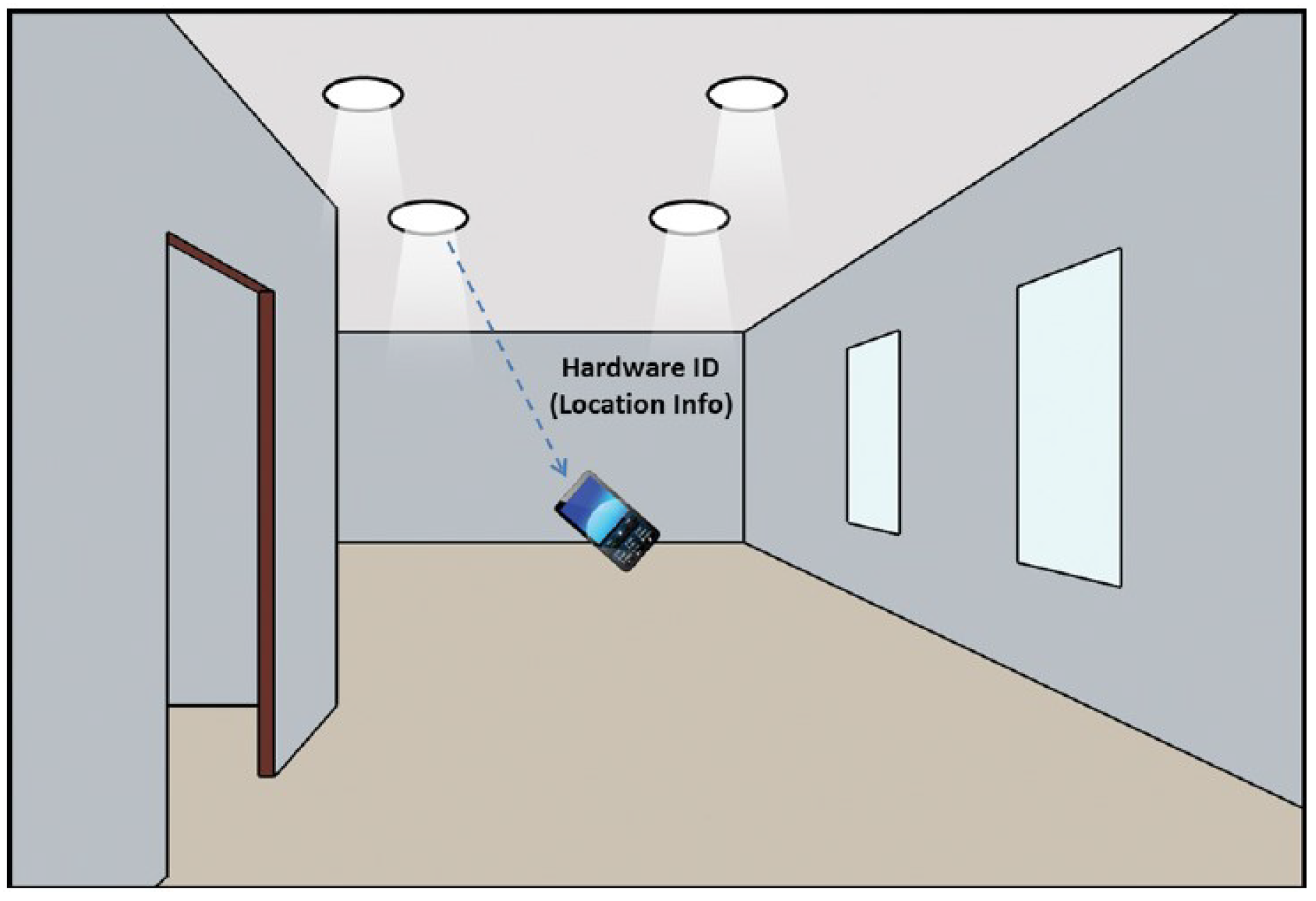
3.13. Visible Light Communication (VLC)
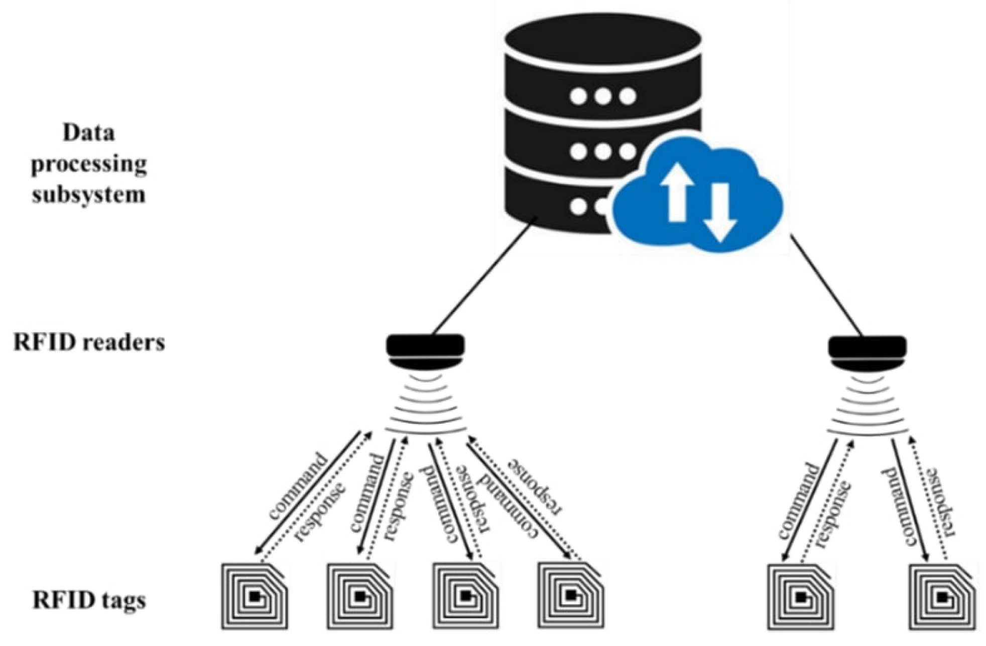
3.14. Radio Frequency Identification (RFID)
3.15. Acoustic
3.16. Ultrasound
3.17. Infrared Radiation (IR)
4. Discussion
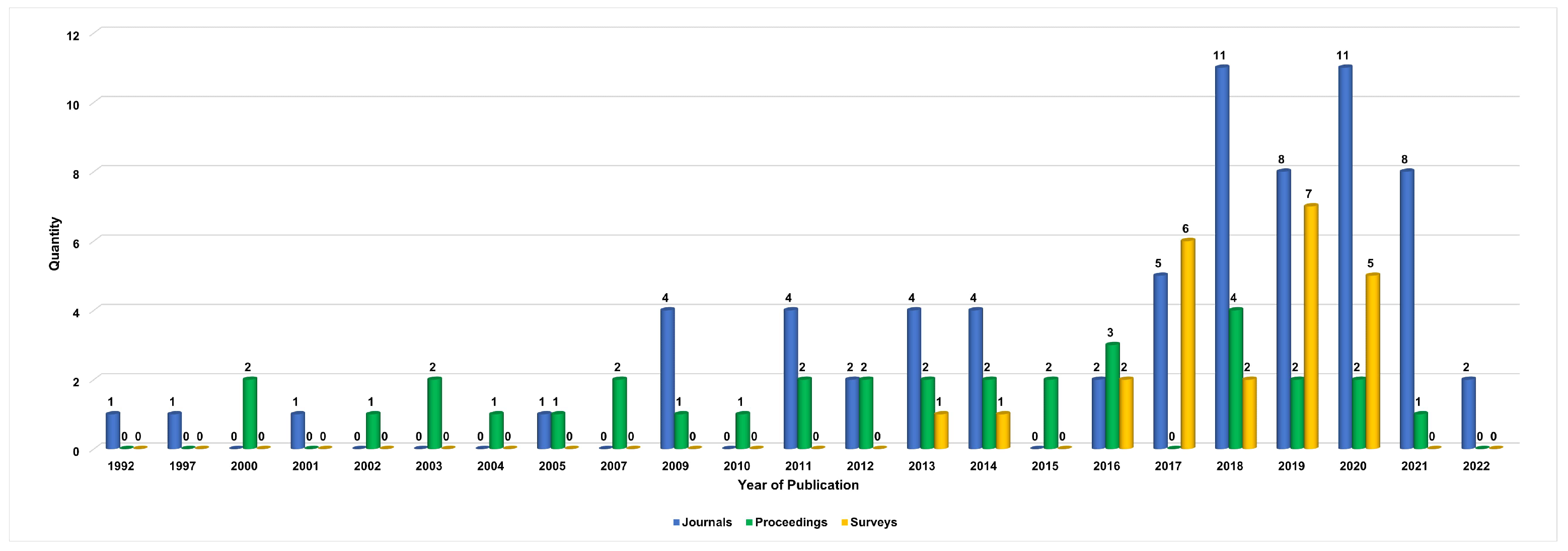
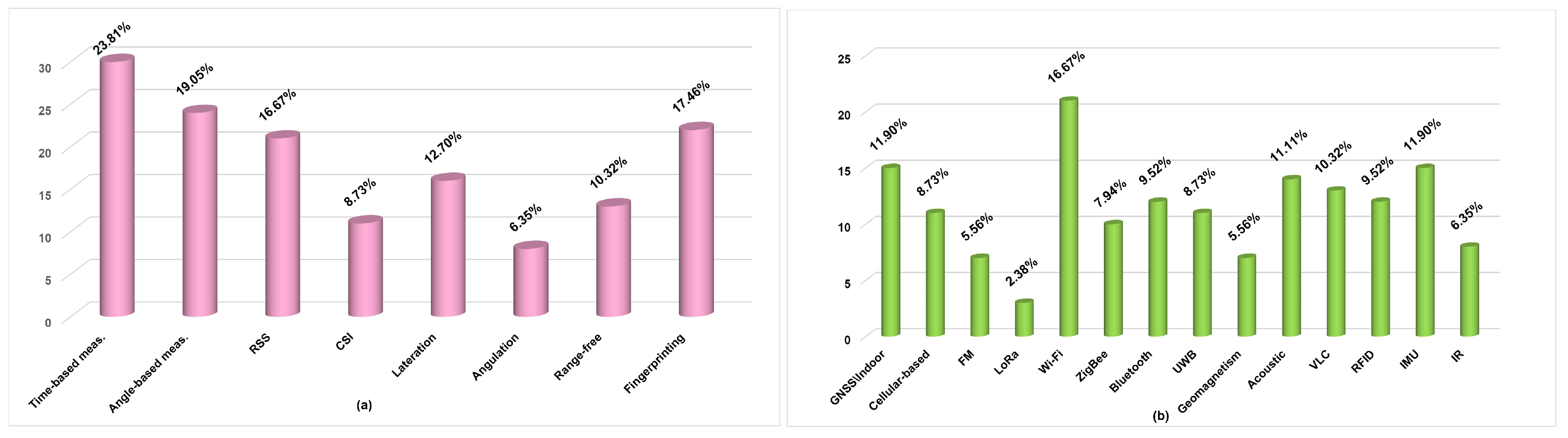
4.1. Statistical Analysis
4.2. Design Parameters
4.3. Future Directions
4.3.1. Fusion of Different Techniques and Technologies
4.3.2. Real-Time World Testing and Deployment
4.3.3. Cloud and Edge Computing
4.3.4. From Smart Sensors to 6G
5. Conclusions
Author Contributions
Funding
Data Availability Statement
Conflicts of Interest
References
- R. and M. Ltd. Global Indoor Location Market by Component (Hardware, Solutions, and Services), Technology (BLE, UWB, Wi-Fi, RFID), Application (Emergency Response Management, Remote Monitoring), Organization Size, Vertical, and Region-Forecast to 2026. Available online: https://www.researchandmarkets.com/reports/5026936/indoor-location-market-by-component-hardware?utm_source=BW&utm_medium=PressRelease&utm_code=cpmnhb (accessed on 28 December 2021).
- Farid, Z.; Nordin, R.; Ismail, M. Recent advances in wireless indoor localization techniques and system. J. Comput. Netw. Commun. 2013. [Google Scholar] [CrossRef]
- Zafari, F.; Papapanagiotou, I.; Devetsikiotis, M.; Hacker, T. An iBeacon based Proximity and Indoor Localization System. arXiv 2017, arXiv:1703.07876. [Google Scholar] [CrossRef]
- Brena, R.F.; García-Vázquez, J.P.; Galván-Tejada, C.E.; Muñoz-Rodriguez, D.; Vargas-Rosales, C.; Fangmeyer, J. Evolution of Indoor Positioning Technologies: A Survey. J. Sens. 2017. [Google Scholar] [CrossRef]
- Garg, V.; Jhamb, M. A Review of Wireless Sensor Network on Localization Techniques. Int. J. Eng. Trends Technol. 2013, 4, 1049–1053. [Google Scholar] [CrossRef]
- Zafari, F.; Gkelias, A.; Leung, K.K. A Survey of Indoor Localization Systems and Technologies. IEEE Commun. Surv. Tutorials 2019, 21, 2568–2599. [Google Scholar] [CrossRef] [Green Version]
- Shakshuki, E.; Abu Elkhail, A.; Nemer, I.; Adam, M.; Sheltami, T. Comparative study on range free localization algorithms. Proc. Procedia Comput. Sci. 2019, 151, 501–510. [Google Scholar] [CrossRef]
- Correa, A.; Barcelo, M.; Morell, A.; Vicario, J.L. A review of pedestrian indoor positioning systems for mass market applications. Sensors 2017, 17, 1927. [Google Scholar] [CrossRef] [Green Version]
- Kanhere, O.; Rappaport, T.S. Position location for futuristic cellular communications: 5G and beyond. IEEE Commun. Mag. 2021, 59, 70–75. [Google Scholar] [CrossRef]
- Akpakwu, G.A.; Silva, B.J.; Hancke, G.P.; Abu-Mahfouz, A.M. A Survey on 5G Networks for the Internet of Things: Communication Technologies and Challenges. IEEE Access 2017, 6, 3619–3647. [Google Scholar] [CrossRef]
- Rastogi, E.; Saxena, N.; Roy, A.; Shin, D.R. Narrowband Internet of Things: A Comprehensive Study. Comput. Netw. 2020, 173, 107209. [Google Scholar] [CrossRef]
- Ma, Y.; Zhou, G.; Wang, S. WiFi sensing with channel state information: A survey. ACM Comput. Surv. 2019, 52, 1–36. [Google Scholar] [CrossRef] [Green Version]
- Liu, M.; Cheng, L.; Qian, K.; Wang, J.; Wang, J.; Liu, Y. Indoor acoustic localization: A survey. Hum.-Centric Comput. Inf. Sci. 2020, 10, 1–24. [Google Scholar] [CrossRef]
- Cobos, M.; Antonacci, F.; Alexandridis, A.; Mouchtaris, A.; Lee, B. A survey of sound source localization methods in wireless acoustic sensor networks. Wirel. Commun. Mob. Comput. 2017. [Google Scholar] [CrossRef] [Green Version]
- Afzalan, M.; Jazizadeh, F. Indoor positioning based on visible light communication: A performance-based survey of real-world prototypes. ACM Comput. Surv. 2019, 52, 1–36. [Google Scholar] [CrossRef]
- Singh, S.P.; Sharma, S.C. Critical Analysis of Distributed Localization Algorithms for Wireless Sensor Networks. Int. J. Wirel. Microw. Technol. 2016, 6, 72–83. [Google Scholar] [CrossRef] [Green Version]
- Ashraf, I.; Hur, S.; Park, Y. Smartphone sensor based indoor positioning: Current status, opportunities, and future challenges. Electronics 2020, 9, 891. [Google Scholar] [CrossRef]
- Jin-Shyan, L.; Yu-Wei, S.; Shen, C.C. A Comparative Study of Wireless Protocols: Bluetooth, UWB, ZigBee and Wi-Fi. In Proceedings of the 33rd Annual Conference of the IEEE Industrial Electronics Society (IECON), Taipei, Taiwan, 5–8 November 2007. [Google Scholar]
- Jang, B.; Kim, H. Indoor positioning technologies without offline fingerprinting map: A survey. IEEE Commun. Surv. Tutorials 2019, 21, 508–525. [Google Scholar] [CrossRef]
- Khudhair, A.A.; Jabbar, S.Q.; Sulttan, M.Q.; Wang, D. Wireless indoor localization systems and techniques: Survey and comparative study. Indones. J. Electr. Eng. Comput. Sci. 2016, 3, 392–409. [Google Scholar] [CrossRef] [Green Version]
- Liu, J.; Jain, R. Survey of Wireless Based Indoor Localization Technologies; Department of Science and Engineering, Washington University: St. Louis, MO, USA, 2014. [Google Scholar]
- Alsinglawi, B.; Elkhodr, M.; Nguyen, Q.V.; Gunawardana, U.; Maeder, A.; Simoff, S. RFID localisation for internet of things smart homes: A survey. Int. J. Comput. Netw. Commun. 2017, 9, 81–99. [Google Scholar] [CrossRef]
- Bai, Y.; Lu, L.; Cheng, J.; Liu, J.; Chen, Y.; Yu, J. Acoustic-based sensing and applications: A survey. Comput. Netw. 2020, 181, 107447. [Google Scholar] [CrossRef]
- Burghal, D.; Ravi, A.T.; Rao, V.; Alghafis, A.A.; Molisch, A.F. A Comprehensive Survey of Machine Learning Based Localization with Wireless Signals. arXiv 2020, arXiv:2012.11171. [Google Scholar]
- Jeon, K.E.; She, J.; Soonsawad, P.; Ng, P.C. BLE Beacons for Internet of Things Applications: Survey, Challenges, and Opportunities. IEEE Internet Things J. 2018, 5, 811–828. [Google Scholar] [CrossRef]
- Luo, J.; Fan, L.; Li, H. Indoor Positioning Systems Based on Visible Light Communication: State of the Art. IEEE Commun. Surv. Tutorials 2017, 19, 2871–2893. [Google Scholar] [CrossRef]
- Nessa, A.; Adhikari, B.; Hussain, F.; Fernando, X.N. A Survey of Machine Learning for Indoor Positioning. IEEE Access 2020, 8, 214945–214965. [Google Scholar] [CrossRef]
- Parihar, M.S.I.; Asutkar, G.M.; Chaturvedi, S. Performance Evaluation Of Wireless Sensor Network (WSN) In 5G Infrastructure: A Review. Nagpur Int. J. Innov. Eng. Sci. 2019, 4, 8. [Google Scholar]
- Saeed, N.; Nam, H.; Al-Naffouri, T.Y.; Alouini, M.S. A State-of-the-Art Survey on Multidimensional Scaling Based Localization Techniques. IEEE Commun. Surv. Tutor. 2019, arXiv:1906.03585. [Google Scholar] [CrossRef] [Green Version]
- Hashem, O.; Harras, K.A.; Youssef, M. Accurate indoor positioning using IEEE 802.11mc round trip time. Pervasive Mob. Comput. 2021, 75, 101416. [Google Scholar] [CrossRef]
- Harter, A.; Hopper, A.; Steggles, P.; Ward, A.; Webster, P. The anatomy of a context-aware application. In Proceedings of the 5th Annual ACM/IEEE International Conference on Mobile Computing and Networking, Seattle, WA, USA, 15–19 August 1999; pp. 59–68. [Google Scholar]
- Priyantha, N.B.; Chakraborty, A.; Balakrishnan, H. The cricket location-support system. In Proceedings of the 6th Annual International Conference on Mobile Computing and Networking, Boston, MA, USA, 6–11 August 2000; pp. 32–43. [Google Scholar]
- Peng, C.; Shen, G.; Zhang, Y.; Li, Y.; Tan, K. BeepBeep: A High Accuracy Acoustic Ranging System Using COTS Mobile Devices. In Proceedings of the 5th International Conference on Embedded Networked Sensor Systems, Sydney Australia; Association for Computing Machinery, New York, NY, USA, 6–9 November 2007; pp. 1–14. [Google Scholar] [CrossRef]
- Si, M.; Wang, Y.; Xu, S.; Sun, M.; Cao, H. A Wi-Fi FTM-based indoor positioning method with LOS/NLOS identification. Appl. Sci. 2020, 10, 956. [Google Scholar] [CrossRef] [Green Version]
- Zhang, Y.; Duan, L. A phase-difference-of-arrival assisted ultra-wideband positioning method for elderly care. Meas. J. Int. Meas. Confed. 2021, 170, 108689. [Google Scholar] [CrossRef]
- Mohanna, M.; Rabeh, M.L.; Zieur, E.M.; Hekala, S. Optimization of MUSIC algorithm for angle of arrival estimation in wireless communications. NRIAG J. Astron. Geophys. 2013, 2, 116–124. [Google Scholar] [CrossRef] [Green Version]
- Oumar, O.A.; Siyau, M.F.; Sattar, P.T. Comparison between MUSIC and ESPRIT Direction of Arrival Estimation Algorithms for Wireless Communication Systems. In The First International Conference on Future Generation Communication Technologies, London, UK; IEEE: New York, NY, USA, 2012; ISBN 9781467358613. [Google Scholar]
- Joana Halder, S.; Kim, W. A fusion approach of RSSI and LQI for indoor localization system using adaptive smoothers. J. Comput. Netw. Commun. 2012, 2012, 1–10. [Google Scholar] [CrossRef]
- Maiajner, M.; Gleich, D. Study of Link Quality Indicator for Possible usage in Angle of Arrival Estimation. In Proceedings of the International Conference on Systems, Signals and Image Processing, Bangalore, India, 8–10 January 2014. [Google Scholar]
- Wang, J.J.; Hwang, J.G.; Park, J.G. A novel indoor ranging algorithm based on received signal strength and channel state information. In Proceedings of the IPIN (Short Papers/Work-in-Progress Papers), Pisa, Italy, 30 September–3 October 2019; pp. 32–39. [Google Scholar]
- Bahl, P.; Padmanabhan, V. RADAR: An in-building RF-based user location and tracking system. In Proceedings of the IEEE INFOCOM 2000, Conference on Computer Communications. Nineteenth Annual Joint Conference of the IEEE Computer and Communications Societies (Cat. No.00CH37064), Tel Aviv, Israel, 26–30 March 2000; Volume 2, pp. 775–784. [Google Scholar] [CrossRef]
- Fang, S.H.; Cheng, Y.C.; Chien, Y.R. Exploiting Sensed Radio Strength and Precipitation for Improved Distance Estimation. IEEE Sens. J. 2018, 18, 6863–6873. [Google Scholar] [CrossRef]
- Stefanski, J. Hyperbolic Position Location Estimation in the Multipath Propagation Environment. In Proceedings of the Joint IFIP Wireless and Mobile Networking Conference, Gdansk, Poland, 9–11 September 2009. [Google Scholar] [CrossRef] [Green Version]
- Huynh, P.; Yoo, M. VLC-based positioning system for an indoor environment using an image sensor and an accelerometer sensor. Sensors 2016, 16, 783. [Google Scholar] [CrossRef] [PubMed] [Green Version]
- Patil, S.; Zaveri, M. MDS and Trilateration Based Localization in Wireless Sensor Network. Wirel. Sens. Netw. 2011, 3, 198–208. [Google Scholar] [CrossRef] [Green Version]
- Song, Q.; Guo, S.; Liu, X.; Yang, Y. CSI Amplitude fingerprinting-based NB-IoT indoor localization. IEEE Internet Things J. 2018, 5, 1494–1504. [Google Scholar] [CrossRef]
- Costa, J.A.; Patwari, N.; Hero Iii, A.O. Distributed Weighted-Multidimensional Scaling for Node Localization in Sensor Networks. ACM Trans. Sens. Netw. TOSN 2006, 2, 39–64. [Google Scholar] [CrossRef] [Green Version]
- Qi, X.; Liu, X.; Liu, L. A Combined Localization Algorithm for Wireless Sensor Networks. Math. Probl. Eng. 2018, 2018, 1–10. [Google Scholar] [CrossRef]
- Risteska Stojkoska, B. Nodes Localization in 3D Wireless Sensor Networks Based on Multidimensional Scaling Algorithm. Int. Sch. Res. Not. 2014, 2014, 1–10. [Google Scholar] [CrossRef] [PubMed]
- Liu, Y.; Yi, X.; He, Y. A novel centroid localization for wireless sensor networks. Int. J. Distrib. Sens. Netw. 2012, 2012, 8. [Google Scholar] [CrossRef]
- Cheikhrouhou, O.; Bhatti, G.M.; Alroobaea, R. A hybrid DV-hop algorithm using RSSI for localization in large-scale wireless sensor networks. Sensors 2018, 18, 1469. [Google Scholar] [CrossRef] [Green Version]
- Jian Yin, L.; Elhoseny, M. A New Distance Vector-Hop Localization Algorithm Based on Half-Measure Weighted Centroid. Mob. Inf. Syst. 2019, 2019, 1–9. [Google Scholar] [CrossRef]
- Payal, A. Analysis and Implementation of APIT Localization Algorithm for Wireless Sensor Network. In Proceedings of the 3rd International Conference on Computer and Communication Systems (ICCCS), Nagoya, Japan, 27–30 April 2018; Institute of Electrical and Electronics Engineers Inc.: New York City, NY, USA; pp. 306–309. [Google Scholar] [CrossRef]
- Chen, S.T.; Zhang, C.; Li, P.; Zhang, Y.Y.; Jiao, L.B. An indoor Collaborative Coefficient-triangle APIT localization algorithm. Algorithms 2017, 10, 131. [Google Scholar] [CrossRef] [Green Version]
- Michaelides, M.P.; Panayiotou, C.G. SNAP: Fault tolerant event location estimation in sensor networks using binary data. IEEE Trans. Comput. 2009, 58, 1185–1197. [Google Scholar] [CrossRef]
- Janiesch, C.; Zschech, P.; Heinrich, K. Machine learning and deep learning. Electron. Mark. 2021, 31, 685–695. [Google Scholar] [CrossRef]
- Wu, L.; Chen, C.H.; Zhang, Q. A mobile positioning method based on deep learning techniques. Electronics 2019, 8, 59. [Google Scholar] [CrossRef] [Green Version]
- Potortì, F.; Torres-Sospedra, J.; Quezada-Gaibor, D.; Jiménez, A.R.; Seco, F.; Pérez-Navarro, A.; Ortiz, M.; Zhu, N.; Renaudin, V.; Ichikari, R.; et al. Off-line evaluation of indoor positioning systems in different scenarios: The experiences from IPIN 2020 competition. IEEE Sens. J. 2021, 22, 5011–5054. [Google Scholar] [CrossRef]
- Potorti, F.; Park, S.; Crivello, A.; Palumbo, F.; Girolami, M.; Barsocchi, P.; Lee, S.; Torres-Sospedra, J.; Ruiz, A.R.J.; Pérez-Navarro, A.; et al. The IPIN 2019 indoor localisation competition—Description and results. IEEE Access 2020, 8, 206674–206718. [Google Scholar] [CrossRef]
- Norrdine, A. An Algebraic Solution to the Multilateration Problem. In Proceedings of the 2012 International Conference on Indoor Positioning and Indoor Navigation, IPIN 2012, Sydney, Australia, 13–15 November 2012. [Google Scholar]
- Aernouts, M.; Berkvens, R.; Van Vlaenderen, K.; Weyn, M. Sigfox and LoRaWAN Datasets for Fingerprint Localization in Large Urban and Rural Areas. Data 2018, 3, 13. [Google Scholar] [CrossRef]
- Accuware Video Tracker. 2015. Available online: http://public.accuware.com/files/Accuware_Video_Tracker_Fact_Sheet.pdf (accessed on 1 September 2021).
- NXP. Available online: https://www.nxp.com/applications/enabling-technologies/connectivity/ultra-wideband-uwb:UWB (accessed on 21 May 2022).
- Poulose, A.; Eyobu, O.S.; Han, D.S. An indoor position-estimation algorithm using smartphone IMU sensor data. IEEE Access 2019, 7, 11165–11177. [Google Scholar] [CrossRef]
- Xu, S.; Chen, R.; Yu, Y.; Guo, G.; Huang, L. Locating Smartphones Indoors Using Built-In Sensors and Wi-Fi Ranging with an Enhanced Particle Filter. IEEE Access 2019, 7, 95140–95153. [Google Scholar] [CrossRef]
- Guvenc, I.; Dedeoglu, O. Enhancements to RSS Based Indoor Tracking Systems Using Kalman Filters. In Proceedings of the International Signal Processing Conference (ISPC) and Global Signal, Dallas, TX, USA, 31 March–3 April 2003. [Google Scholar]
- Chris Woodford. Explain that Stuff, 2021. Available online: https://www.explainthatstuff.com/how-roomba-works.html (accessed on 20 November 2021).
- Kaiser, S. Successive collaborative slam: Towards reliable inertial pedestrian navigation. Information 2020, 11, 464. [Google Scholar] [CrossRef]
- YouTube. Geospatialmedia, 2017. Available online: https://www.youtube.com/watch?v=CCKisghkcA4&t=161s (accessed on 10 January 2021).
- Khelifi, F.; Bradai, A.; Benslimane, A.; Rawat, P.; Atri, M. A Survey of Localization Systems in Internet of Things. Mob. Netw. Appl. 2019, 24, 761–785. [Google Scholar] [CrossRef]
- Borio, D.; Gioia, C. Indoor Navigation Using Asynchronous Pseudolites. In Proceedings of the 6th European Workshop on GNSS Signals and Signal Processing, Noordwijk, The Netherlands, 5–7 December 2012. [Google Scholar] [CrossRef]
- Ma, C.; Yang, J.; Chen, J.; Tang, Y. Indoor and outdoor positioning system based on navigation signal simulator and pseudolites. Adv. Space Res. 2018, 62, 2509–2517. [Google Scholar] [CrossRef]
- Schröder, Y.; Wolf, L. A Low-Cost GNSS Repeater for Indoor Operation. In Proceedings of the 4th KuVS/GI Expert Talk on Localization, Lübeck, Germany, 11–12 July 2019. [Google Scholar] [CrossRef]
- Lashiley. GNSS solutions: Repeaters, Pseudolites and Indoor Positioning. Inside GNSS Magazine, July/August 09. Available online: https://www.insidegnss.com/auto/julyaug09-GNSS-Sol.pdf (accessed on 20 December 2021).
- Selmi, I.; Samama, N.; Vervisch-Picois, A. A new approach for decimeter accurate GNSS indoor positioning using carrier phase measurements. In Proceedings of the 2013 International Conference on Indoor Positioning and Indoor Navigation, IPIN, Montbeliard, France, 28–31 October 2013; IEEE Computer Society: Washington, DC, USA, 2013. [Google Scholar] [CrossRef]
- Samama, N.; Vervisch-Picois, A.; Taillandier-Loize, T. A GNSS-based inverted radar for carrier phase absolute indoor positioning purposes first experimental results with GPS signals. In Proceedings of the 2016 International Conference on Indoor Positioning and Indoor Navigation, IPIN, Alcala de Henares, Spain, 4–7 October 2016; Institute of Electrical and Electronics Engineers Inc.: New York City, NY, USA, 2016. [Google Scholar] [CrossRef]
- ETSI. GSM Global System for Mobile Communications; Technical Report; ETSI TC-SMG: 1996. Available online: https://portal.etsi.org/tb/closed_tb/closed_smg/smg.asp (accessed on 21 February 2021).
- Vukmirović, N.; Janjić, M.; Djurić, P.M.; Erić, M. Position estimation with a millimeter-wave massive MIMO system based on distributed steerable phased antenna arrays. Eurasip J. Adv. Signal Process. 2018, 2018, 33. [Google Scholar] [CrossRef] [PubMed]
- Björnson, E.; Sanguinetti, L.; Wymeersch, H.; Hoydis, J.; Marzetta, T.L. Massive MIMO is a reality—What is next?: Five promising research directions for antenna arrays. Digit. Signal Process. 2019, 94, 3–20. [Google Scholar] [CrossRef]
- Weng, Z.K.; Kanno, A.; Dat, P.T.; Inagaki, K.; Tanabe, K.; Sasaki, E.; Kürner, T.; Jung, B.K.; Kawanishi, T. Millimeter-Wave and Terahertz Fixed Wireless Link Budget Evaluation for Extreme Weather Conditions. IEEE Access 2021, 9, 163476–163491. [Google Scholar] [CrossRef]
- Garcia, N.; Wymeersch, H.; Larsson, E.G.; Haimovich, A.M.; Coulon, M. Direct localization for massive MIMO. IEEE Trans. Signal Process. 2017, 65, 2475–2487. [Google Scholar] [CrossRef] [Green Version]
- Lin, X. An Overview of 5G Advanced Evolution in 3GPP Release 18. IEEE Commun. Stand. Mag. 2022, 6, 77–83. [Google Scholar] [CrossRef]
- Wu, Q.; Zhang, S.; Zheng, B.; You, C.; Zhang, R. Intelligent Reflecting Surface-Aided Wireless Communications: A Tutorial. IEEE Trans. Commun. 2021, 69, 3313–3351. [Google Scholar] [CrossRef]
- Sejan, M.A.S.; Rahman, M.H.; Shin, B.S.; Oh, J.H.; You, Y.H.; Song, H.K. Machine Learning for Intelligent-Reflecting-Surface-Based Wireless Communication towards 6G: A Review. Sensors 2022, 22, 5405. [Google Scholar] [CrossRef]
- Liu, S.; Gao, Z.; Zhang, J.; Di Renzo, M.; Alouini, M.S. Deep denoising neural network assisted compressive channel estimation for mmWave intelligent reflecting surfaces. IEEE Trans. Veh. Technol. 2020, 69, 9223–9228. [Google Scholar] [CrossRef]
- Özdoğan, Ö.; Björnson, E. Deep learning-based phase reconfiguration for intelligent reflecting surfaces. In Proceedings of the 54th Asilomar Conference on Signals, Systems, and Computers, IEEE, Virtual Conference, 1–4 November 2020; pp. 707–711. [Google Scholar]
- Budge, M.C.; German, S.R. Basic Radar Analysis; Atech House radar series; Artech House: Boston, MA, USA; London, UK, 2015. [Google Scholar]
- Moreira, A.; Prats-Iraola, P.; Younis, M.; Krieger, G.; Hajnsek, I.; Papathanassiou, K.P. A tutorial on synthetic aperture radar. IEEE Geosci. Remote. Sens. Mag. 2013, 1, 6–43. [Google Scholar] [CrossRef] [Green Version]
- Mondini, A.C.; Guzzetti, F.; Chang, K.T.; Monserrat, O.; Martha, T.R.; Manconi, A. Landslide failures detection and mapping using Synthetic Aperture Radar: Past, present and future. Earth-Sci. Rev. 2021, 216, 103574. [Google Scholar] [CrossRef]
- de Wit, J.J.M.; van Rossum, W.L.; de Jong, A.J. Orthogonal waveforms for FMCW MIMO radar. In Proceedings of the 2011 IEEE RadarCon (RADAR), Kansas City, MO, USA, 23–27 May 2011; pp. 686–691. [Google Scholar] [CrossRef]
- Schimel, A.; Beaudoin, J.; Parnum, I.; Le Bas, T.; Schmidt, V.; Keith, G. Multibeam sonar backscatter data processing. Mar. Geophys. Res. 2018, 39, 121–137. [Google Scholar] [CrossRef]
- Yin, C.; Dimitrios, L.; Jie, L.; Bodhi, P. FM-based Indoor Localization. In Proceedings of the 10th International Conference on Mobile Systems, Applications, and Services, Low Wood Bay, Lake District, UK, 25–29 June 2012; p. 534. [Google Scholar]
- Augustin, A.; Yi, J.; Clausen, T.; Townsley, W.M. A study of Lora: Long range & low power networks for the internet of things. Sensors 2016, 16, 1466. [Google Scholar] [CrossRef]
- Sigfox Atlas | Sigfox Build. Available online: https://build.sigfox.com/geolocation-sigfox-atlas (accessed on 1 September 2022).
- Popleteev, A. Improving ambient FM indoor localization using multipath-induced amplitude modulation effect: A year-long experiment. Pervasive Mob. Comput. 2019, 58, 101022:1–101022:14. [Google Scholar] [CrossRef]
- Pereira, C.; Guenda, L.; Carvalho, N.B. A Smart-Phone Indoor/Outdoor Localization System. In Proceedings of the 2016 International Conference on Indoor Positioning and Indoor Navigation, IPIN, Madrid, Spain, 4–7 October 2016; pp. 21–23. [Google Scholar]
- Vasisht, D.; Kumar, S.; Katabi, D. Decimeter-Level Localization with a Single WiFi Access Point. In Proceedings of the 13th USENIX Symposium on Networked Systems Design and Implementation (NSDI 16), Santa Clara, CA, USA, 16–18 March 2016; pp. 165–178. [Google Scholar]
- Pipelidis, G.; Tsiamitros, N.; Kessner, M.; Prehofer, C. HuMAn: Human Movement Analytics via WiFi Probes. In Proceedings of the IEEE International Conference on Pervasive Computing and Communications Workshops (PerCom Workshops), Kyoto, Japan, 11–15 March 2019; pp. 370–372. [Google Scholar] [CrossRef]
- Ibrahim, M.; Liu, H.; Jawahar, M.; Nguyen, V.; Gruteser, M.; Howard, R.; Yu, B.; Bai, F. Verification: Accuracy evaluation of WiFi fine time measurements on an open platform. In Proceedings of the of the Annual International Conference on Mobile Computing and Networking, MOBICOM. Association for Computing Machinery, New Delhi, India, 29 October–2 November 2018; pp. 417–427. [Google Scholar] [CrossRef]
- Hernandez, O.; Jain, V.; Chakravarty, S.; Bhargava, P. Position Location Monitoring Using IEEE® 802.15.4/ZigBee® technology. Beyond Bits 2009, 4, 67–69. [Google Scholar]
- Lin, Y.W.; Lin, C.Y. An interactive real-time locating system based on bluetooth low-energy beacon network. Sensors 2018, 18, 1637. [Google Scholar] [CrossRef] [PubMed] [Green Version]
- Ruiz, A.R.J.; Granja, F.S. Comparing Ubisense, BeSpoon, and DecaWave UWB Location Systems: Indoor Performance Analysis. IEEE Trans. Instrum. Meas. 2017, 66, 2106–2117. [Google Scholar] [CrossRef]
- Ultra Wideband availability. Available online: https://support.apple.com/en-us/HT212274 (accessed on 4 April 2022).
- Lee, S.; Chae, S.; Han, D. Iloa: Indoor localization using augmented vector of geomagnetic field. IEEE Access 2020, 8, 184242–184255. [Google Scholar] [CrossRef]
- Renaudin, V.; Combettes, C. Magnetic, acceleration fields and gyroscope quaternion (MAGYQ)-based attitude estimation with smartphone sensors for indoor pedestrian navigation. Sensors 2014, 14, 22864–22890. [Google Scholar] [CrossRef] [PubMed] [Green Version]
- Ashraf, I.; Hur, S.; Park, Y. MagIO: Magnetic field strength based indoor- outdoor detection with a commercial smartphone. Micromachines 2018, 9, 534. [Google Scholar] [CrossRef] [PubMed]
- Gozick, B.; Subbu, K.P.; Dantu, R.; Maeshiro, T. Magnetic maps for indoor navigation. IEEE Trans. Instrum. Meas. 2011, 60, 3883–3891. [Google Scholar] [CrossRef]
- Li, Y.; Ghassemlooy, Z.; Tang, X.; Lin, B.; Zhang, Y. A VLC Smartphone Camera Based Indoor Positioning System. IEEE Photonics Technol. Lett. 2018, 30, 1171–1174. [Google Scholar] [CrossRef]
- Zhang, B.; Zhang, Q.; Wang, Y.; Tian, Z. The method of solving the non-coplanar perspective-four-point (P4P) problem. In Proceedings of the 33rd Chinese Control Conference, CCC, Kunming, China, 22–24 May 2021; IEEE Computer Society: Washington, DC, USA, 2014; pp. 1039–1043. [Google Scholar] [CrossRef]
- Authority, A. Google Maps’ new Visual Positioning System Fixes Navigation. Available online: https://www.androidauthority.com/google-maps-visual-positioning-system-navigation-863139/ (accessed on 1 September 2022).
- I. Stojmenovic. Handbook of Sensor Networks: Algorithms and Architectures; Wiley-Interscience: Hoboken, NJ, USA, 2005. [Google Scholar]
- Naz, A.; Hassan, N.U.; Pasha, M.A.; Asif, H.; Jadoon, T.M.; Yuen, C. Single LED ceiling lamp based indoor positioning system. In Proceedings of the IEEE World Forum on Internet of Things, WF-IoT 2018–Proceedings, Singapore, 5–8 February 2018; Institute of Electrical and Electronics Engineers Inc.: New York City, NY, USA, 2018; Volume 2018, pp. 682–687. [Google Scholar] [CrossRef]
- Zhang, W.; Chowdhury, M.I.S.; Kavehrad, M. Asynchronous indoor positioning system based on visible light communications. Optical Eng. 2014, 53, 045105. [Google Scholar] [CrossRef]
- Kavehrad, M.; Aminikashani, R. Visible Light Communication Based Indoor Localization; CRC Press Taylor & Francis Group: Boca Raton, FL, USA, 2020. [Google Scholar]
- Hou, Y.; Xue, Y.; Chen, C.; Xiao, S. A RSS/AOA based indoor positioning system with a single LED lamp. In Proceedings of the 2015 International Conference on Wireless Communications and Signal Processing, WCSP, Nanjing, China, 15–17 October 2015; Institute of Electrical and Electronics Engineers Inc.: New York City, NY, USA, 2015. [Google Scholar] [CrossRef]
- Wang, T.Q.; Sekercioglu, Y.A.; Neild, A.; Armstrong, J. Position accuracy of time-of-arrival based ranging using visible light with application in indoor localization systems. J. Light. Technol. 2013, 31, 3302–3308. [Google Scholar] [CrossRef]
- Ni, L.M.; Liu, Y.; Lau, Y.C.; Patil, A.P. LANDMARC: Indoor Location Sensing Using Active RFID. Wirel. Netw. 2004, 10, 701–710. [Google Scholar] [CrossRef]
- Ni, L.M.; Zhang, D.; Souryal, M.R. RFID-based localization and tracking technologies. IEEE Wirel. Commun. 2011, 18, 45–51. [Google Scholar] [CrossRef]
- Wang, J.; Katabi, D. Dude, Where’s My Card? RFID Positioning That Works with Multipath and Non-Line of Sight. In Proceedings of the ACM SIGCOMM 2013 Conference on SIGCOMM, Hong Kong, China, 12–16 August 2013. [Google Scholar] [CrossRef]
- Mandai, A.; Lopes, C.V.; Givargis, T.; Haghighat, A.; Jurdak, R.; Baldi, P. Beep: 3D indoor positioning using audible sound. In Proceedings of the 2005 2nd IEEE Consumer Communications and Networking Conference, CCNC2005, Las Vegas, NV, USA, 6 January 2005; Volume 2005, pp. 348–353. [Google Scholar] [CrossRef]
- Ward, A.; Jones, A.; Hopper, A. A New Location Technique for the Active Office. IEEE Pers. Commun. 1997, 4, 42–47. [Google Scholar] [CrossRef] [Green Version]
- Fukuju, Y.; Minami, M.; Morikawa, H.; Aoyama, T. DOLPHIN: An autonomous indoor positioning system in ubiquitous computing environment. In Proceedings of the IEEE Workshop on Software Technologies for Future Embedded Systems, WSTFES, Hokkaido, Japan, 15–16 May 2003; Institute of Electrical and Electronics Engineers Inc.: New York City, NY, USA, 2003; pp. 53–56. [Google Scholar] [CrossRef]
- Lucas, J. What Is Infrared? 2019. Available online: https://www.livescience.com/50260-infrared-radiation.html (accessed on 14 July 2022).
- Lee, S. Use of infrared light reflecting landmarks for localization. Ind. Robot. 2009, 36, 138–145. [Google Scholar] [CrossRef]
- Sakai, N.; Zempo, K.; Mizutani, K.; Wakatsuki, N. Linear positioning system based on ir beacon and angular detection photodiode array. In Proceedings of the International Conference on Indoor Positioning and Indoor Navigation (IPIN), Alcalá de Henares, Spain, 4–7 October 2016; pp. 4–7. [Google Scholar]
- Yang, D.; Xu, B.; Rao, K.; Sheng, W. Passive Infrared (PIR)-Based Indoor Position Tracking for Smart Homes Using Accessibility Maps and A-Star Algorithm. Sensors 2018, 18, 332. [Google Scholar] [CrossRef] [Green Version]
- Schwendemann, J.; Müller, T.; Krautschneider, R. Indoor navigation of machines and measuring devices with iGPS. In Proceedings of the 2010 International Conference on Indoor Positioning and Indoor Navigation, IPIN 2010, Zurich, Switzerland, 15–17 September 2010. [Google Scholar] [CrossRef]
- Do, T.H.; Yoo, M. TDOA-based indoor positioning using visible light. Photonic Netw. Commun. 2014, 27, 80–88. [Google Scholar] [CrossRef]
- Othman, R.; Gaafar, A.; Muaaz, L.; Elsayed, M.H. A Hybrid RSS+AOA Indoor Positioning Algorithm Based on Visible Light Communication. In Proceedings of the 2020 International Conference on Computer, Control, Electrical, and Electronics Engineering, ICCCEEE, Khartoum, Sudan, 26 February–1 March 2020; Institute of Electrical and Electronics Engineers Inc.: New York City, NY, USA, 2021. [Google Scholar] [CrossRef]
- Wu, K.; Xiao, J.; Yi, Y.; Chen, D.; Luo, X.; Ni, L.M. CSI-based indoor localization. IEEE Trans. Parallel Distrib. Syst. 2013, 24, 1300–1309. [Google Scholar] [CrossRef] [Green Version]
- Höflinger, F.; Bordoy, J.; Simon, N.; Wendeberg, J.; Reindl, L.M.; Schindelhauer, C. Indoor-localization system for smart phones. In Proceedings of the 2015 IEEE International Workshop on Measurements and Networking, M and N, Coimbra, Portugal, 12–13 October 2015; Institute of Electrical and Electronics Engineers Inc.: New York City, NY, USA, 2015; pp. 59–64. [Google Scholar] [CrossRef]
- General Data Protection Regulation (GDPR)—Official Legal Text. Available online: https://gdpr-info.eu (accessed on 26 January 2021).
- Want, R.; Hopper, A.; Falcao, V.; Gibbons, J. The Active Badge Location System. ACM Trans. Sens. Netw. (TOSN) 1992, 10, 99–102. [Google Scholar] [CrossRef]
- Rappaport, T.S.; Xing, Y.; Kanhere, O.; Ju, S.; Madanayake, A.; Mandal, S.; Alkhateeb, A.; Trichopoulos, G.C. Wireless Communications and Applications Above 100 GHz: Opportunities and Challenges for 6G and Beyond. IEEE Access 2019, 7, 78729–78757. [Google Scholar] [CrossRef]
- OpenStreetMap. Available online: https://www.openstreetmap.org/ (accessed on 26 February 2021).
- Khanh, T.T.; Nguyen, V.; Pham, X.Q.; Huh, E.N. Wi-Fi indoor positioning and navigation: A cloudlet-based cloud computing approach. Hum.-Centric Comput. Inf. Sci. 2020, 10, 1–26. [Google Scholar] [CrossRef]
- Liu, X.; Guo, L.; Yang, H.; Wei, X. Visible Light Positioning Based on Collaborative LEDs and Edge Computing. IEEE Trans. Comput. Soc. Syst. 2021, 9, 324–335. [Google Scholar] [CrossRef]
- Saily, M.; Yilmaz, O.N.C.; Michalopoulos, D.S.; Perez, E.; Keating, R.; Schaepperle, J. Positioning Technology Trends and Solutions Toward 6G. In Proceedings of the 2021 IEEE 32nd Annual International Symposium on Personal, Indoor and Mobile Radio Communications (PIMRC), Helsinki, Finland, 13–16 September 2021; IEEE: Helsinki, Finland, 2021; pp. 1–7. [Google Scholar] [CrossRef]
- Bourdoux, A.; Barreto, A.N.; van Liempd, B.; de Lima, C.; Dardari, D.; Belot, D.; Lohan, E.S.; Seco-Granados, G.; Sarieddeen, H.; Wymeersch, H.; et al. 6G White Paper on Localization and Sensing. arXiv 2020, arXiv:2006.01779. [Google Scholar]
- Aladsani, M.; Alkhateeb, A.; Trichopoulos, G.C. Leveraging mmWave Imaging and Communications for Simultaneous Localization and Mapping. arXiv 2018, arXiv:1811.07097. [Google Scholar]


| Wireless Technologies | |||||||||||||
|---|---|---|---|---|---|---|---|---|---|---|---|---|---|
| Techniques | GNSS/Indoor | FM | LoRa | Wi-Fi | ZigBee | Bluetooth | RF | UWB | Geomagnetism | VLC | RFID | Acoustic | IR |
| ToA | [72,73] [74,75] | [97] | [32] [47] | [102] | [113] [116] | [31,32] [33,121] | |||||||
| TDoA | [74,76] [127] | [122] | [102] | [112] [128] | [122] | ||||||||
| RTT | [30,99] | [101] | |||||||||||
| PDoA | [35] | ||||||||||||
| AoA | [36,37] [78,81] [39] | [115] [129] | |||||||||||
| LQI | [39] | ||||||||||||
| RSS | [71] | [30,34] [66] | [100] | [41,55] [47,51] [49] | [35] | [115] [129] | [117] | ||||||
| CSI | [46] | [130] | [119] | ||||||||||
| Lateration | [48] | [120] | |||||||||||
| Hyperbolic | [74,76] [127] | [122] | [102] | [112] [128] | [122] | ||||||||
| Angulation | [36,37] [78,81] [39] | [115] [129] | |||||||||||
| Fingerprinting | [96] | [92] [95] | [61] | [41,92] [96] | [61] | [104] [107] | [117] | ||||||
| APIT | [50,53] [54] | ||||||||||||
| DV-Hop | [51,52] | ||||||||||||
| MDS | [45,49] [48] | ||||||||||||
| SNAP | [55] | ||||||||||||
| PDR/IMU | [65,66] | [44] | |||||||||||
| Filters | [3] | [106] | [131] | [105] | |||||||||
| SLAM | [68] | ||||||||||||
Disclaimer/Publisher’s Note: The statements, opinions and data contained in all publications are solely those of the individual author(s) and contributor(s) and not of MDPI and/or the editor(s). MDPI and/or the editor(s) disclaim responsibility for any injury to people or property resulting from any ideas, methods, instructions or products referred to in the content. |
© 2023 by the authors. Licensee MDPI, Basel, Switzerland. This article is an open access article distributed under the terms and conditions of the Creative Commons Attribution (CC BY) license (https://creativecommons.org/licenses/by/4.0/).
Share and Cite
Isaia, C.; Michaelides, M.P. A Review of Wireless Positioning Techniques and Technologies: From Smart Sensors to 6G. Signals 2023, 4, 90-136. https://doi.org/10.3390/signals4010006
Isaia C, Michaelides MP. A Review of Wireless Positioning Techniques and Technologies: From Smart Sensors to 6G. Signals. 2023; 4(1):90-136. https://doi.org/10.3390/signals4010006
Chicago/Turabian StyleIsaia, Constantina, and Michalis P. Michaelides. 2023. "A Review of Wireless Positioning Techniques and Technologies: From Smart Sensors to 6G" Signals 4, no. 1: 90-136. https://doi.org/10.3390/signals4010006