1. Introduction
Acoustic scattering by multiple objects is an interesting problem with various practical applications. The simplest realistic problem of multiple scattering by finite bodies appears to be that by two spheres. Many publications on this subject can be found in [
1,
2,
3,
4,
5,
6,
7,
8,
9,
10,
11,
12,
13,
14,
15,
16,
17,
18]. However, an important case of buried scatterers has not been studied in these papers.
In the present paper, the interference of echo-signals from two buried spherical scatterers is investigated. The bottom is assumed to be a homogeneous liquid attenuating half-space. The point source emitting the spherical incident wave of an angular frequency is placed at point of a homogeneous water half-space. Modeling is performed in a wide frequency range of 40–60 kHz. The distance between scatterers and source/receiver is about 100 m.
Generally speaking, the two spheres may be of different sizes. However, for simplicity, later on in the discussions, the two spheres will be assumed to have the same radius.
The spherical scatterers of the same radius
are assumed to be acoustically rigid (i.e., homogeneous Neumann boundary conditions on the outer surface). The distance between their centers is
. The geometry of the problems is depicted in
Figure 1.
The scattering from one sphere in a wide frequency range is determined using the Hackman and Sammelmann’s general approach [
19,
20,
21,
22]. The arising scattering coefficients are evaluated using the steepest descent method [
23,
24].
An alternative and potentially attractive technique for computing the scattering coefficients of the sphere is the method of complex images [
25,
26,
27,
28,
29,
30]. The complex image solution is based on the approximation of the reflection and transmission coefficients via a discrete sum of image point sources, with complex source point coordinates. The two main advantages of this method are its validity in the near field and the existence of a simple recursion relation in frequency [
27] for computing the source parameters. The fitting of the transmission coefficient, which is needed in those configurations where the source is located in one of two media and the scatterer is located in the other medium, is affected by convergence problems which have been reported in the literature [
28]. For this reason, the present work is focused on the steepest descent approximation of the scattering coefficients.
The goal of this paper is to investigate in detail the structure of the interference of the echo-signals from two or more spherical targets submerged in an underwater sediment and evaluate the influence of the Franz type surface wave and water/sediment interface reflections on the form-function.
Computing the far field scattered by objects inside an underwater sediment can be also performed via the Helmholtz–Kirchhoff integral (see, for instance, [
31,
32]).
In [
6] it is shown that in the case of two spherical scatterers in water it is possible to neglect the multiple scattering between scatterers if
. When targets are buried in the attenuating bottom, the condition
is more than sufficient to neglect the multiple scattering between spheres.
All computations and plots in this paper were performed using the computer algebra system Wolfram Mathematica. For special functions, such as spherical Hankel functions or spherical Bessel functions, the built-in functionality is applied.
This paper is organized as follows. In
Section 2, we propose a numerically efficient technique for computing the echo-signal from the only buried spherical target. In
Section 3, modeling of the scattered form-function of the only buried spherical target is carried out and discussed. In
Section 4, we present the results of the numerical calculations of the scattering form-function for two and three spherical scatterers.
Section 5 is the summary of relevant points. Finally,
Section 6 concludes the paper.
2. Echo-Signal from the Only Buried Sphere
Throughout the entire paper, the attention is restricted to harmonic oscillations of constant frequency . The complex time dependence , with representing time, and , is factored out of equations.
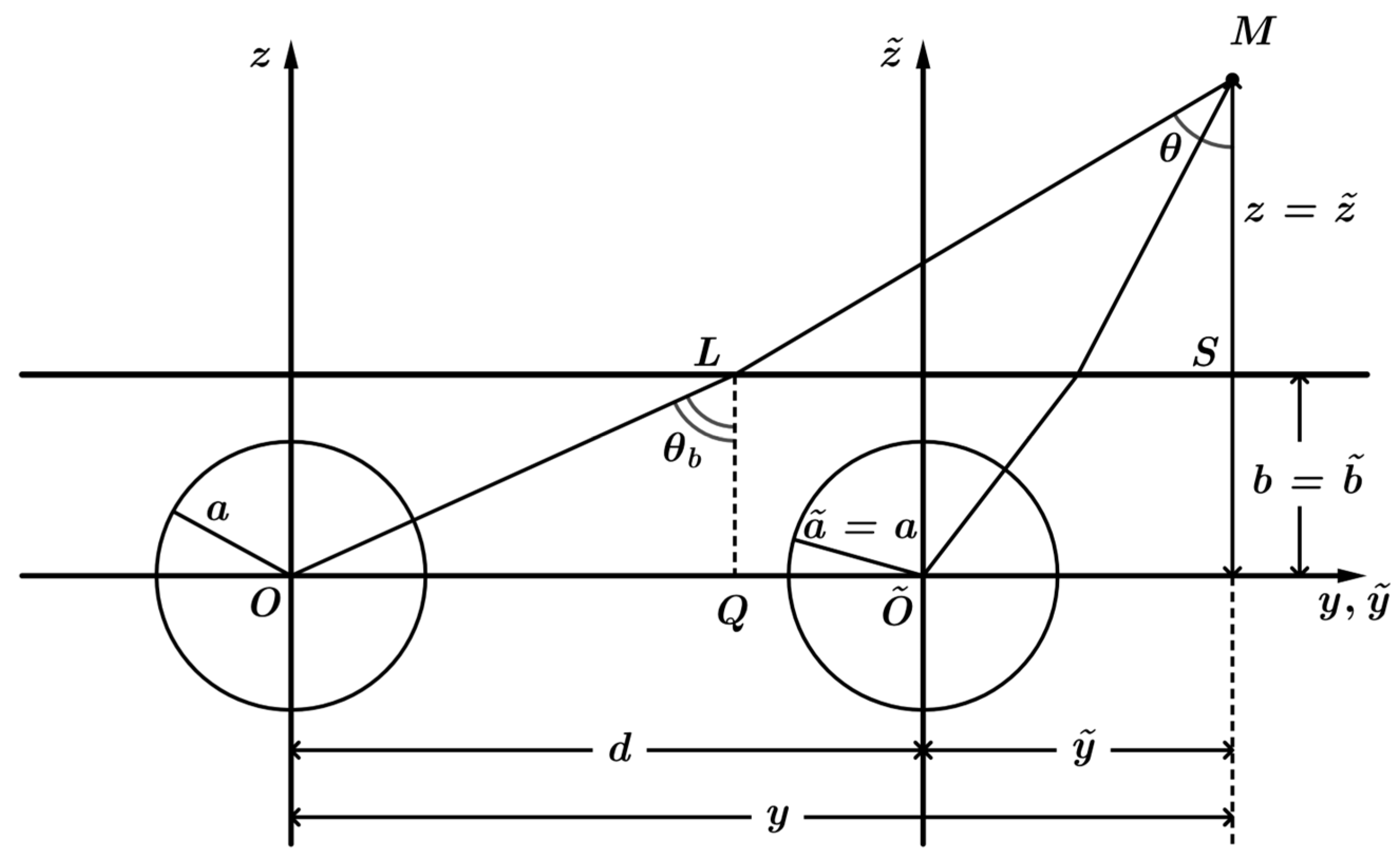
For definiteness, let us consider the scatterer with a center at point
(see
Figure 1). To evaluate the echo-signal from the buried spherical scatterer, let us use the method proposed in [
19,
20,
21,
22], where the acoustic potential of the echo-signal is represented in the form,
In Equation (1),
is the wave number in water, and
are the elements of the free-field T-matrix for the acoustical scattering by the considered target. These elements are found using the separation of variables and applying the appropriate boundary conditions to the spherical harmonics. For the acoustically rigid sphere of a radius
embedded in an underwater sediment,
where,
is the wave number of a longitudinal wave propagating in the bottom,
is the spherical Hankel function of the 1st kind,
is the spherical Bessel function, and the prime marking the spherical functions in Equation (2) indicates a derivative with respect to the whole argument. The scattering coefficients of a sphere
in Equation (1) are as follows:
Here,
for
;
is the cylindrical Bessel function of the
m-th order,
and
are the horizontal and vertical components of the incident vector in water, respectively, and
are the normalized associated Legendre functions of the order
and rank
(see, for example, [
33])
is the plane-wave transmission coefficient for propagation from water to bottom [
24]
Here,
,
. The densities of water and bottom are denoted as
and
, respectively. The following inequalities are assumed to be satisfied in the complex
q-plane:
and
.
In this paper, we will use the single-scatter approximation when
. The full multiple scattering solution modeling the backscattered field from a thin air-filled spherical elastic shell in water close to the seabed or to the air-water interface was studied in [
34].
If the echo-signal from the scatterer is evaluated taking into account the full multiple scattering, the coefficients
in Equation (1) are found using a linear system of algebraic equations (see [
19,
20,
21,
22,
34]). In fact, to find
, it is necessary at each fixed frequency to solve a system of
equations with
unknowns at
, etc., and finally, a system consisting of one equation with one unknown
at
. Coefficients of these systems are integrals with slowly decreasing and rapidly oscillating integrands. This makes computing the coefficients
rather time consuming, and therefore in the present paper we will consider the single-scatter approximation.
The truncation level
in Equation (1) is set by a rule suggested by Kargl and Marston [
35],
where,
is the integer part of
. For
m,
m/s and
kHz, Equation (6) gives
. Thus, computing the backscattered field (1), it will be necessary to sum up more than 4500 summands.
The integral representation of the scattering coefficients (3) is valid for arbitrary frequencies and distances between the source and the target. At frequencies of interest and distances
from 90 m up to 100 m, considered in this paper for illustration, the integrand in (3) is rapidly oscillating and slowly decreasing that makes the straightforward calculation of scattering coefficients rather time consuming. To speed up the computation of integrals (3), we will evaluate them using the steepest descent method (see, for example, [
23,
24]).
Let us change the variable in integral (3), putting
. If
, then
. For
, we have
. Since
,
where,
is the refractive index at the water/bottom interface and
is the ratio of the densities of the bottom and water half-spaces.
Using properties of the Hankel functions
and the associated Legendre functions
, the obtained integral (under the assumption that
) can be written in the form,
where, the integration contour is going along the straight line
from
to 0, then along the real axis from
to
and finally along the straight line
from 0 to
;
is given using Equation (4),
Since, by assumption,
, it is expedient to analyze the integral (8) using the saddle point method (see, for example, [
23,
24]). The saddle point is found from equation,
which can be rewritten in the form,
The incident angle
is connected with the refraction angle
by the equality (the Snell’s law),
From
Figure 1 it follows that,
Thus, the geometrical interpretation of Equation (11) is the validity of equality,
Let us denote the root of Equation (11) via
and the corresponding value of
—via
. Then,
or, using Equation (11),
where,
and
are the lengths of intervals forming the ray going from
to the origin of coordinates
, respectively.
Thus, the estimation of integral (8) by the saddle point method gives,
Here,
The angle is found from Equation (11), and , is the ratio of densities of the bottom and water half-spaces.
Taking account of the second approximation in the saddle point method will add to the expression (12) one more summand of the order . This summand will be only essential at small angles . In this paper, we will consider parameters m, m, and m, when Equation (11) gives rad ().
Our analysis of is complete if angle is less than the angle of total internal reflection . If , it is necessary to take into account the two-valuedness of the function (see Equation (7)) which enters into integral (8). Due to this two-valuedness, in the expression (12) for , an additional term corresponding to the branch cut contribution appears.
Taking into account the representation (12) for the scattering coefficients
, Equation (1) for the acoustic potential of the echo-signal from the sphere will take the form,
The summation theorem for the associated Legendre functions (see [
33]) gives,
Thus,
The obtained formula for the acoustic potential of the echo-signal needs summation only with respect to
. The function B(r) is expressed via elementary functions. This formula is valid for any spherical scatterer: acoustically rigid, elastic, or elastic shells, or to use the proper elements of the T-matrix (for example, the T-matrix elements for a spherical elastic shell filled with air can be found in Appendix A of [
36]).
3. Modeling of the Scattering Form-Function of the Only Buried Spherical Target
To study the frequency dependence of an echo signal, let us consider the form-function of acoustic scattering. In a free water space this function is determined as,
where,
is the acoustic potential of the echo-signal at the reception point and
is the potential of the incident wave at the origin when there is no scatterer (see [
21]).
For the radiated spherical wave and the scattering geometry considered in this paper (see
Figure 1) at
is as follows (see [
23,
24] and the notations used in Equation (3)),
Evaluating this integral as performed to obtain Equation (14), we get,
Finally, for the form-function of the acoustic scattering we get the expression,
In this paper, a medium model with the following parameters is considered: m, m, m, and m. The bottom is assumed to be sandy. The longitudinal wave speed in the bottom m/s, and the sound speed in water m/s. The densities are kg/m3 and kg/m3, respectively. The frequency changes in range of 40–60 kHz.
For the considered scattering geometry of the problem , . Thus .
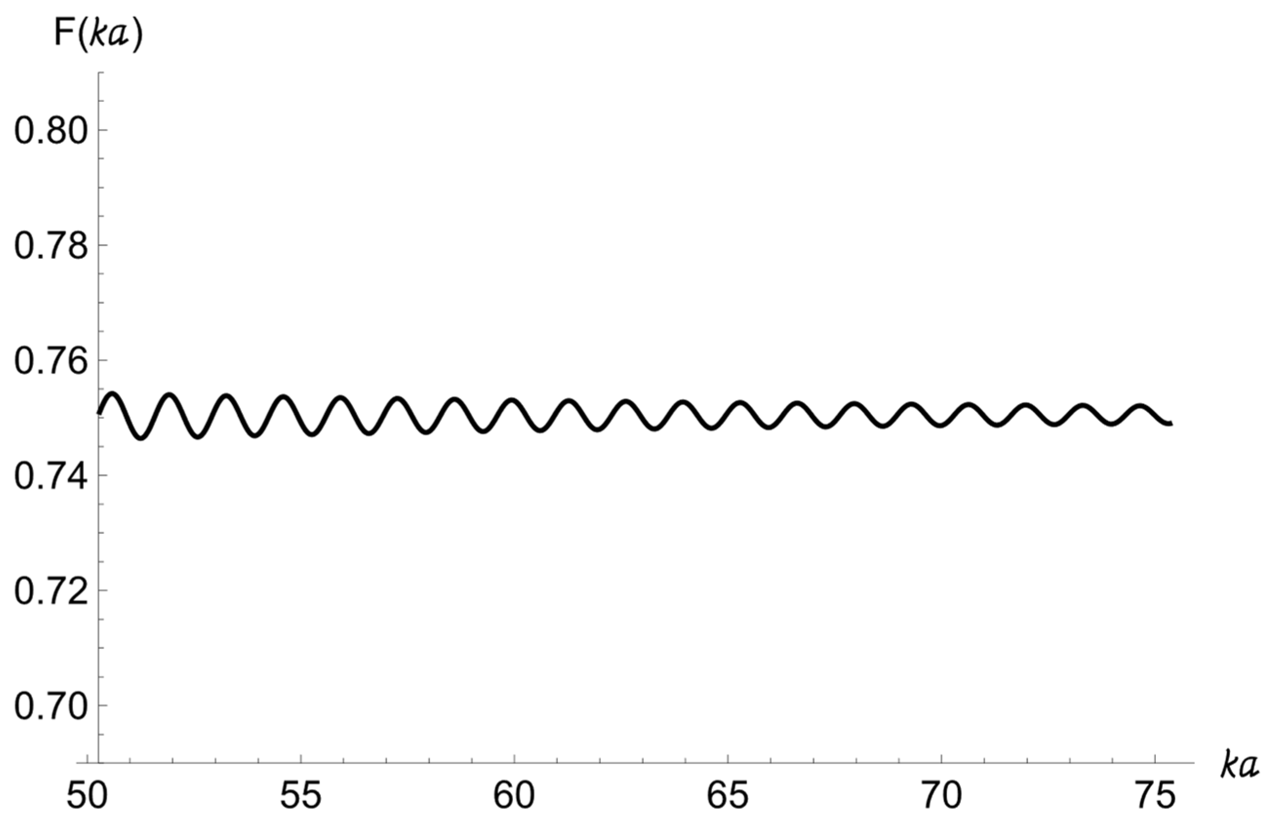
In
Figure 2, the graph of the form-function (17) of the backscattered field from a spherical target of a radius
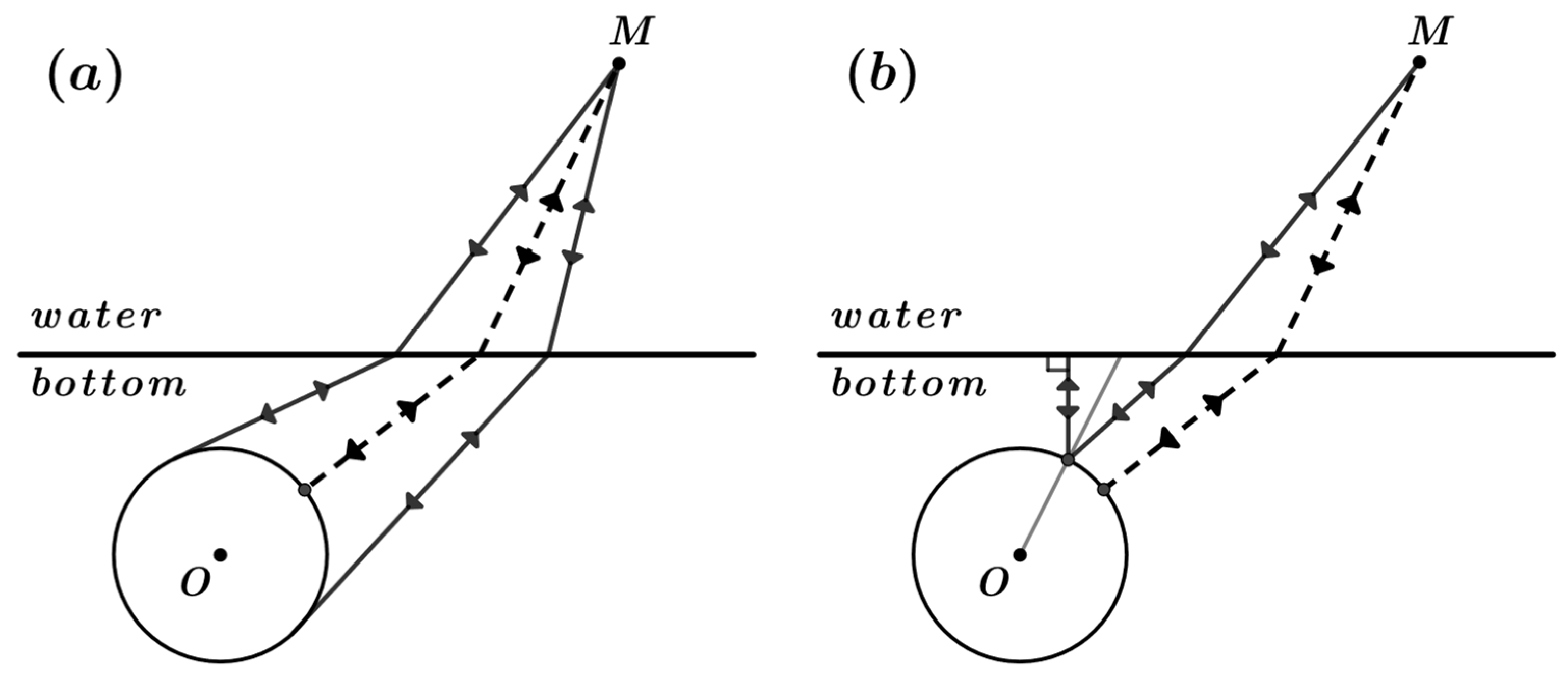
m immersed in a nonattenuating sandy sediment is shown. Since the sphere is considered as a rigid body, there is no wave propagating inside the sphere (no elastic effects) and the scattering problem reduces to a simple reflection problem in the exterior domain for the sphere. In this case, the echo-signal consists of three components: the mirror reflection (see the dashed lines in
Figure 3a,b), the first Franz creeping wave which is exited at the sphere boundary between the illuminated and shadowed parts of the sphere (see the solid line in
Figure 3a), and the wave which is shown by a solid line in
Figure 3b. Additionally, the second Franz wave envelopes the spherical target one more time. As a result, its amplitude essentially decreases and the following Franz waves are not visible on the plot of the scattering form-function. The interference produces oscillations with a period equal to 1.336.
Similar computations were conducted in the case of the absorbing bottom. The bottom attenuation was taken into account by considering as a complex value with m/s. As before, the form-function will be obtained using the Formula (17), where is a complex value .
In
Figure 4, the graph of the form-function (17) of the backscattered field from a spherical target of a radius
m immersed in an attenuating sandy sediment is shown. The decrease observed in the scattering form-function as a function of
is connected with the factor
, where,
and
m.
An approximate value of the form-function obtained using (17) and an exact value calculated using (1)–(4) and (15) for attenuating sandy sediment were compared at several frequencies from the interval kHz. At all these points, the difference between them was of the order of . Thus, the agreement of the exact and asymptotic formulae is excellent.
4. Modeling of Interference of Echo-Signals from Two Spherical Scatterers
The form-function for two spherical scatterers of the same radius
is naturally defined as (see [
6]),
Here,
is the acoustic potential of the sphere with a center at the point
(see
Figure 1), and
is the potential of the incident wave at the origin
when there is no scatterer.
Let us consider two cases:
m (
m,
m) and
m (
m,
m). The graphs of the scattering form-functions for the only buried sphere with
m and
m are shown in
Figure 5.
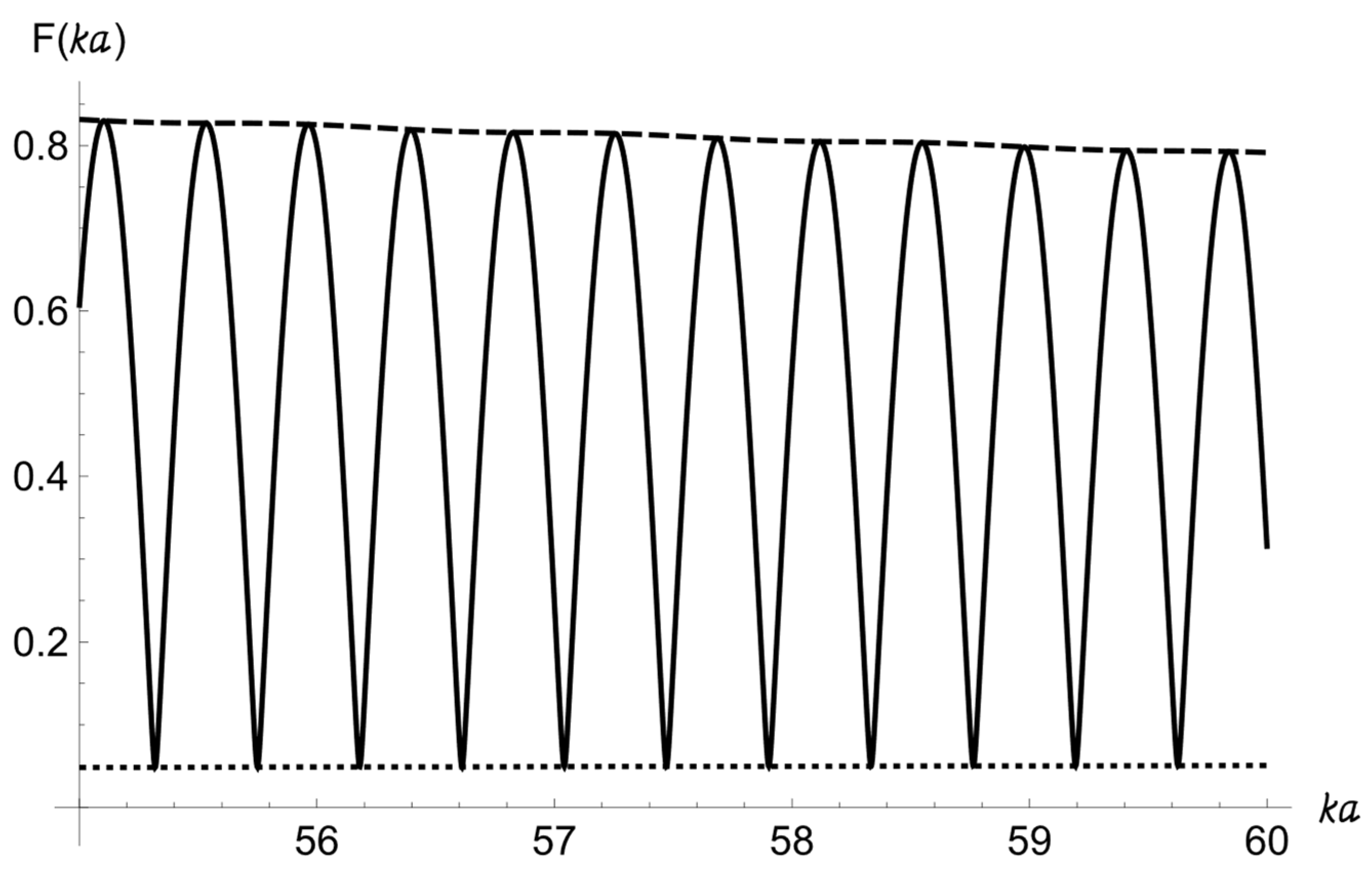
In
Figure 6, the form-function (18) for two spherical targets immersed in an attenuating sediment is shown for
m (
m,
m). The dashed line is the sum of the scattering form-function for the only sphere at
m (see
Figure 4) and the scattering form-function for the only sphere at
m (see the dashed line in
Figure 5). The dotted line is the absolute value of the difference between these two form-functions. The graph of the of the scattering form-function is an oscillating curve with a small period of oscillations. Therefore, we plot these graphs for
.
In
Figure 7, the form-function (18) for two spherical targets buried in an absorbing sandy sediment is shown for
m (
m,
m). The dashed line is the sum of the scattering form-function for the only sphere at
m (see
Figure 4) and the scattering form-function for the only sphere at
m (see solid line in
Figure 5). The dotted line is the absolute value of the difference between these two form-functions.
In
Figure 8, the form-function for two spherical targets buried in an underwater sediment is shown for
m (
m,
m).
Based on the numerical calculations of the backscattered form-function for two spheres with different separation between two spheres and different distances , and , following conclusions may be appropriate:
- (1)
Due to coherent addition of the two signals backscattered from two targets, the upper envelope of the two-sphere scattering form-function is the same as a sum of the form-function curves for each of the two spheres. The lower envelope of the two-sphere scattering form-function is the same as the modulus of the difference between these form-function curves for each of the two spheres.
- (2)
The oscillation period of the two-sphere scattering form-function expressed via
is calculated as,
For m, this period increases about two times (from 0.2141 to 0.4257) when increases from 5 m to 10 m. In case does not change, but the bigger for the pair of spheres changes from m to m, the period of oscillation changes from 0.4251 to 0.4305.
- (3)
The influence of the sphere reflection and water/sediment interface reflection (see
Figure 3a,b, respectively) is not visible on the plots of the form-function because this contribution is too weak to be detected on the curves.
The scattering form-function for three and more spherical scatterers of the same radius
can be defined and calculated similarly to (18). For example, for three targets at
m,
m, and
m, the scattering form-function will be of the form shown in
Figure 9.
The plot of the scattering form-function for these three spherical targets immersed in an attenuating sandy sediment becomes more complicated, i.e., quasiperiodic. The value
increases in comparison with the analogous values for the plots shown in
Figure 6 and
Figure 7.
When the distance between the centers of two spherical scatterers increases, the values of the form-function decrease. When the distance increases to some extent, the three-sphere form-function will be close to the form-function of the nearer spherical target from the source/receiver.
5. Discussion
An efficient method for computing the backscattered field from two or more targets immersed in an absorbing underwater sediment has been presented. In simulations, the targets are assumed to be spherical of radius and acoustically rigid. The bottom is assumed to be a homogeneous liquid attenuating half-space. The transmitter/receiver is located in a homogeneous water half-space. The distances between the transmitter/receiver and objects of interest are supposed to be large compared to the acoustic wavelengths in water and sediment.
For calculation of the echo-signal from the only buried sphere, we have followed the Hackman and Sammelmann’s general approach. The arising scattering coefficients of the sphere were evaluated using the steepest descent method. The use of the obtained asymptotic expansions also allowed to essentially decrease the number of summands in the formula for the form-function of the backscattered acoustic field. The computational examples demonstrate efficiency of the presented technique.
The obtained asymptotic formula for the form-function can be used for the elastic target or the spherical elastic shell as well. In this case, it will only be necessary to replace elements of the free-field T-matrix.
In the case of the only acoustically rigid spherical scatterer, the echo-signal consists of three components: the mirror reflection, the Franz creeping wave which is exited at the sphere boundary between the illuminated and shadowed parts of the sphere, and the wave reflected from the water/non-absorbing sand interface. Taking into account the attenuation in the sediment, provides results depending essentially on the geometry of the problem (on depth of the scatterer and the length of the ray path propagating in a seabed).
The two spherical scattering form-function is an oscillation curve with a small period of oscillations. The oscillation period of the two sphere form-function expressed via is obtained using (19). The upper envelope is the same as a sum of the form-function curves from each of the two spheres. The lower envelope of the two-sphere form-function is the same as the modulus of the difference between these form-function curves for each of the two spheres.
At
m and
m, the periods calculated using this formula and the oscillation periods of the curves in
Figure 5 and
Figure 6 coincide with the accuracy of
.
Simulations held for three spherical targets showed more complicated (quasiperiodic) behavior of the plot of the scattering form-function, especially if the distance between two neighboring scatterers is not constant.

 and
and 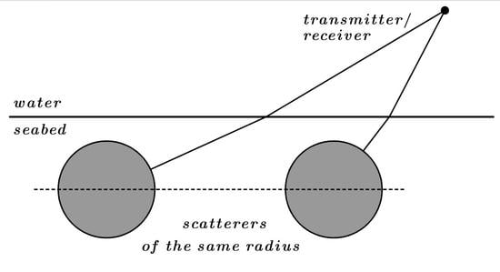


