Article

Key Factors That Influence the Frequency Range of Measured Leak Noise in Buried Plastic Water Pipes: Theory and Experiment

by
Oscar Scussel
1,*,
Michael J. Brennan
1,2,3,
Fabrício Cézar L. de Almeida
3,
Mauricio K. Iwanaga
2,
Jennifer M. Muggleton
1,
Phillip F. Joseph
1 and
Yan Gao
4
1
Institute of Sound and Vibration Research, University of Southampton, Highfield Rd., Southampton SO17 1BJ, UK
2
Department of Mechanical Engineering, UNESP-FEIS, Ilha Solteira, São Paulo 15385-000, Brazil
3
Department of Mechanical Engineering, UNESP-FEB, Bauru, São Paulo 17033-360, Brazil
4
Key Laboratory of Noise and Vibration Research, Institute of Acoustics, Chinese Academy of Sciences, Beijing 100190, China
*
Author to whom correspondence should be addressed.
Acoustics 2023, 5(2), 490-508; https://doi.org/10.3390/acoustics5020029
Submission received: 20 March 2023 / Revised: 7 May 2023 / Accepted: 10 May 2023 / Published: 12 May 2023
(This article belongs to the Special Issue Vibration and Noise)

Abstract

:
The frequency range of the leak noise in buried water pipes, measured using acoustic correlators, depends significantly on the type of pipe and its location as well as the type of sensors used. Having a rough idea of this frequency range can be beneficial for operators prior to conducting tests; however, there is currently no method of predicting it except through practical experience, and no model-based approach yet exists. This issue is addressed in the present paper by using a concise and relatively simple analytical model of the water-pipe–soil system combined with the sensors’ frequency response. The influence of the various physical parameters of the system, such as the pipe and soil properties and the sensor type, on the cross-power spectral density (CPSD) of leak noise signals and, furthermore, the frequency range are investigated. The main factors that affect the bandwidth are the distance between the sensors, wave speed of the predominantly fluid-borne wave in the pipe and the attenuation of this wave. It is shown that the external medium has a profound effect on the propagation and, in turn, on the bandwidth. The approach to predicting this bandwidth is validated using experimental data from three different test sites.

1. Introduction

Wastage of water from distribution systems due to leaks and many other causes is a prevalent problem across the world. For example, in the USA, about 16% of water is lost on average [1]; in Europe, it varies between countries, but, on average, it is about 23% [2]; and in Brazil, it is about 38%, but in eight states, the loss is greater than 50% [3]. In 2014, São Paulo was within 20 days of running out of water due to draught conditions [4], as was Cape Town, South Africa, in 2018 [5]. Other cities such as Mexico City, Melbourne and Jakarta are considered to be at risk [5], as are many states in India [6].
In 2016, the UK Water Industry Research Association (UKWIR) commissioned a series of studies to investigate ways of achieving zero leakage by 2050. Five reports were produced on this topic in 2017 [7], one which concerns leak detection and location using acoustic methods, to which the reader is referred for a literature survey on this problem, along with a comprehensive review provided by Puust et al. [8]. This paper uses a specific technique for locating leaks, which involves using a leak noise correlator. These devices have been in use for several years [9] and measure acoustic pressure in a pipe or pipe vibrations at convenient access points located on either side of a leak. The maximum point in the cross-correlation of the measured signals provides the time difference between the arrival of the leak noise at the sensors’ locations. This information is combined with the sensors’ spacing to determine the position of the leak [10].
As the leak noise travels along the pipe wall towards the sensors, it is filtered, and the frequency response characteristic of the sensor further affects the shape of the leak noise spectrum. The filtering effect of the pipe and the sensors combined acts as a low-pass filter or a band-pass filter, depending on the sensors used [11,12]. After the publication of these articles, there have been developments in creating more comprehensive models that consider the effects of the surrounding soil [13,14], and investigated experimentally [15].
Recently, attempts have been made to improve the location of leaks using signal processing techniques with different levels of complexity. Alternative ways of extracting the leak noise signals from measured data have involved artificial neural networks and machine-learning-based approaches [16,17,18], wavelet transform [19,20], and variational mode decomposition [21,22,23]. The majority of research conducted on water leak detection emphasizes the significance of estimating the frequency bandwidth that contains leak noise features; however, currently, there is no model-based method to predict such a bandwidth, which can vary significantly depending on factors such as the pipe material, location, surrounding soil and type of sensors utilized. For practical purposes, it is beneficial for operators of leak noise correlators to have an estimate of this frequency range prior to conducting field tests. Currently, the only way to obtain such an estimate is by performing field measurements, which can be a tedious and challenging process requiring a specialized experimental setup. This paper proposes a solution to this issue by developing a simple analytical model of the water-pipe–soil system coupled with the frequency response of the sensors.
This aim of this paper is to examine the ways in which the physical parameters of a buried or submerged plastic water pipe can impact the bandwidth of the leak noise. This investigation includes both a theoretical analysis, using an analytical model, and analyses of experimental data sets from three different regions around the world to assess the accuracy of the model in estimating the frequency range of the measured leak noise. A concise overview of the main findings of this research has been presented in the proceedings of a conference in [24]. Here, a detailed description of the theory is given in turn, including in-depth discussion towards the key factors affecting the bandwidth of the leak noise.
The paper is organised as follows: In Section 2, an overview of leak detection using noise correlators is provided to show the role of the cross-power spectral density (CPSD) function between the measured signals in this process. A discussion on how to define the bandwidth of the leak noise, using the CPSDs presented in Section 2, is given in Section 3. Following this, Section 4 derives closed-form solutions for the frequency bandwidth of the measured leak noise from an in vacuo water-filled pipe. Section 5 extends the concept presented in Section 4 to the case where the pipe is surrounded by an external medium. Section 6 reports some experimental results, before the paper is closed with some conclusions in Section 7. There is also an Appendix to the paper (Appendix A), which details an analytical model of the buried/submerged plastic water pipe.

2. Overview of Leak Detection Using Cross-Correlation

Figure 1 shows a typical situation in which noise generated by a leak is used to pinpoint the leak using an acoustic correlator. Vibration or acoustic sensors are generally attached to convenient access points on either side of the suspected leak position. An expression for the leak position d 1 from the left-hand sensor shown in Figure 1 is d 1 = d c T 0 / 2 [10], where c is the speed of propagation of the leak noise, d = d 1 + d 2 is the total distance between the sensors, and T 0 = d 2 d 1 / c is the difference in arrival times of the leak noise at the sensor positions (time delay). The time delay is the quantity measured in leak noise correlators, which is estimated using the cross-correlation function (CCF), which, in turn, is related to the CPSD. Once the time delay has been estimated, it can be combined with knowledge of the velocity of the leak noise propagation in the pipe to pinpoint the position of the leak. In plastic pipes, leak noise is propagated in the form of a predominantly fluid wave that is strongly coupled to the radial motion of the pipe wall [14,15,25,26], a model of which is given in the Appendix A.
The CCF, R x 1 x 2 τ , between the two measured signals x 1 t and x 2 t , is used to estimate the time delay T 0 . It is given by [10]
R x 1 x 2 τ = F 1 S x 1 x 2 ω = 1 2 π + S x 1 x 2 ω e j ω τ d ω ,
where F 1 is the inverse Fourier transform, S x 1 x 2 ω is the CPSD between the measured signals, ω is the circular frequency and j = 1 . The time delay estimate between the measured signals x 1 t and x 2 t is given by a distinct peak in the CCF. For a pure time delay, the gradient of the phase of the CPSD is equal to T 0 .

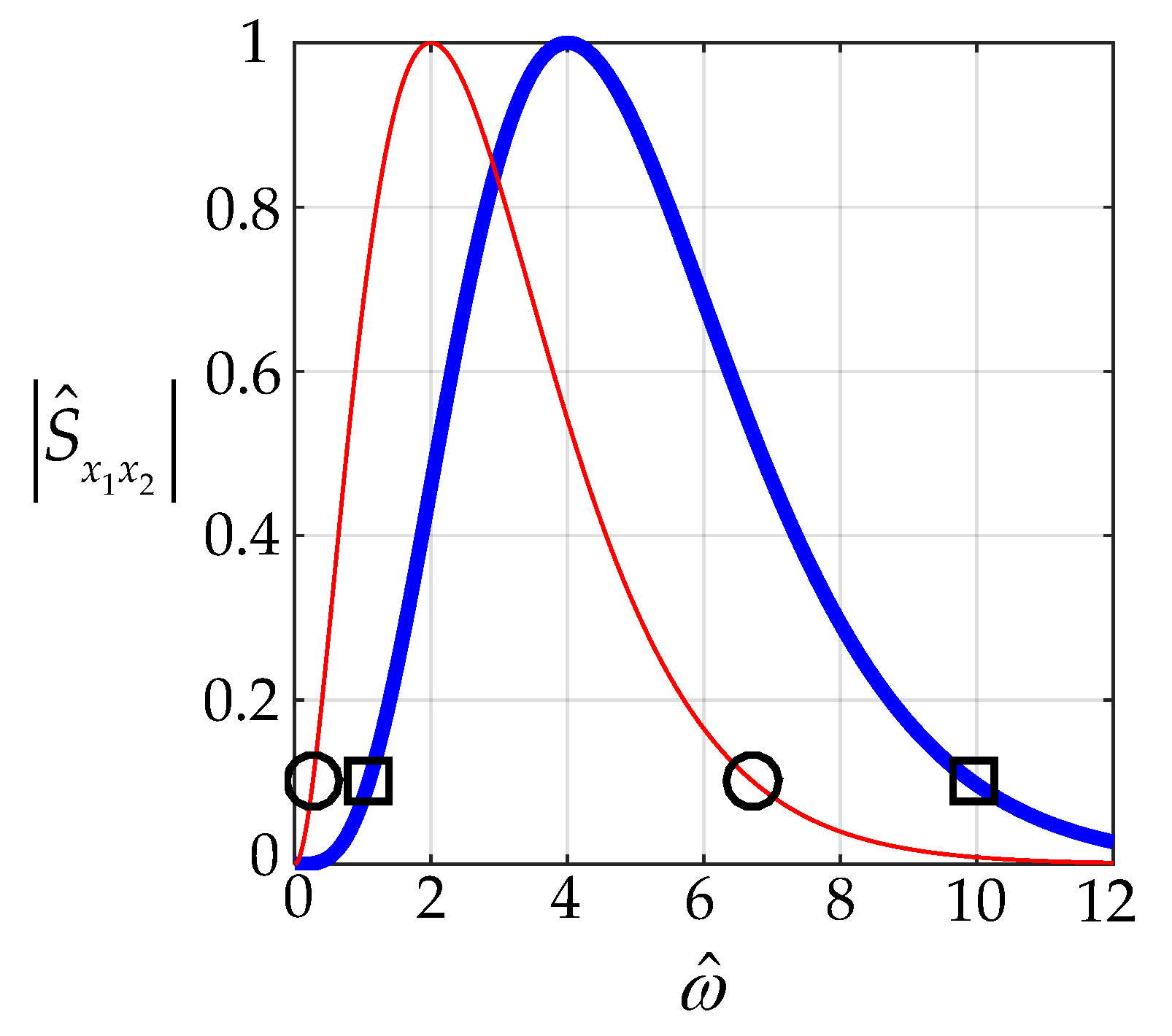
3. Defining the Frequency Bandwidth of Measured Leak Noise

The frequency bandwidth of the measured leak noise from the two measurements can be determined from the CPSD, which, for pressure measurements, is given by [27]
S x 1 x 2 ω = S L ω H * ( ω , d 1 ) H ( ω , d 2 ) ,
where the superscript * denotes the complex conjugate and S L ω is the flat spectrum of the leak noise. The term H ω , d i = e j k d i   ( i = 1   or   2 ) is the frequency response function (FRF) between the acoustic pressure at the position of the leak and the acoustic pressure at the measurement point, in which k = ω / c is the wavenumber related to propagation of the leak noise in the pipe, which is derived in Appendix A. The FRF can also be written as H ω , d i = e ω β d i e j ω d i / c , where β = Im k / ω gives the attenuation of the leak noise as it travels along the pipe wall, and c = ω / Re k . Thus, for acoustic pressure measurements inside the pipe
S x 1 x 2 ( p ) ω = S L ω e ω β d e j ω T 0 ,
where the superscript (p) denotes a pressure measurement. For velocity and acceleration measurements of the pipe wall, the CPSDs are respectively given by [11]
S x 1 x 2 ( v ) ω = A v 2 ω 2 S L ω e ω β d e j ω T 0 and
S x 1 x 2 ( a ) ω = A a 2 ω 4 S L ω e ω β d e j ω T 0 ,
where the superscripts (v) and (a) denote the velocity and acceleration measurements, respectively. The constants A v and A a are related to the properties of the pipe and can be arbitrarily set to 1 in this paper without loss of generalisation. The moduli of Equation (2b,d) can be written in non-dimensional form as
S ^ x 1 x 2 ( p ) ω ^ = e ω ^ ,
S ^ x 1 x 2 ( v ) ω ^ = ω ^ 2 e ω ^ 2 2 e 2 ,   and
S ^ x 1 x 2 ( a ) ω ^ = ω ^ 4 e ω ^ 2 8 e 4 ,
where ω ^ = ω β d . Note that the maximum value of each of Equation (3a–c) is unity. Note also that for both velocity and acceleration measurements, the combination of the FRFs for the transducer and the FRFs for the pipe results in a band-pass filter [11]. To illustrate the filtering behaviour of the pipe system, Equation (3b,c) is plotted in Figure 2 for a water-filled massless pipe with no surrounding medium (in vacuo). For this type of system both β and c are constants, so the peak of the CPSD occurs at a non-dimensional frequency of 2 for velocity measurements and 4 for acceleration measurements [28]. The band-pass characteristics of the systems are evident. Additionally, shown in the figure are two circles and squares, which indicate the limits of the band-pass filter for a 10 dB drop from the maximum peak for velocity and acceleration data, respectively.

4. Calculating the Frequency Bandwidth of Measured Leak Noise in an In Vacuo Water-Filled Pipe

In the special case of a massless in vacuo water-filled pipe, it is possible to derive closed-form approximate expressions for the upper and lower frequencies of the band-pass filter effect of the pipe and transducer combination. To determine the bandwidth of the filter, the minimum value of S ^ x 1 x 2 ω ^ that defines the lower and upper cut-off frequencies needs to be chosen, and then the corresponding non-dimensional frequencies ω ^ lower and ω ^ upper can be determined. Letting S ^ x 1 x 2 ω ^ lower = S ^ x 1 x 2 ω ^ upper = μ , and then taking the square root of Equation (3b) and the 4th root of Equation (3c), results in
ω ^ 2 e ω ^ 2 = μ 1 2 e 1   and
ω ^ 4 e ω ^ 4 = μ 1 4 e 1 ,
for velocity and acceleration measurements, respectively. For the specific case of a massless in vacuo water-filled pipe, β = β 0 and c = c 0 are constants, i.e., they are frequency independent, which means that Equation (4a,b) can be further manipulated. It can be seen that these equations are of the form f z = z e z = α . To determine ω ^ lower and ω ^ upper , it is necessary to find the solution z = f 1 α , which is, in fact, the Lambert W function, i.e., z = W α , named after Johann Heinrich Lambert [29,30]. This function has many applications in science and mathematics, some of which are described in [30,31] along with an interesting discussion about the function. The solutions of Equation (4a,b) can be estimated by calculating the Lambert W function of the term on the right-hand side of each equation. Thus, the upper and lower frequencies of the band-pass filter are given by
ω ^ lower ,   upper = r W α ,
where r = 2 and α = μ 1 2 / e 1 for velocity measurements, and r = 4 and α = μ 1 4 / e 1 . For the problem in hand, the Lambert W function has two values corresponding to the lower and upper cut-off frequencies of the band-pass filter characterising the system. Equation (5) can be solved using in-built Lambert W functions in programs such as Matlab®, or can be solved iteratively by noting that z = ln α ln z (note, however, that this only converges to the upper cut-off frequency). Alternatively, approximate closed-form solutions can be determined from series expansions of the Lambert W functions [30]. For velocity and acceleration measurements, the lower and upper cut-off frequencies are, respectively given by
ω ^ lower r α + α 2 + 3 2 α 3   and
ω ^ upper r ln α ln ln α + ln ln α ln α .
Note that for μ = 0.1 , which is the level set in Figure 2, the non-dimensional lower and upper cut-off frequencies are given by 0.27 and 6.73, respectively, for the velocity measurements, and 1.09 and 9.95, respectively, for the acceleration measurements. The errors in the approximations for the lower and upper cut-off frequencies determined using Equation (6a,b) are −0.5% and −2.7%, respectively, for the velocity measurements, and −3.1% and −6.7%, respectively, for the acceleration measurements.
The above analysis has shown that the bandwidth of measured leak noise in a massless in vacuo pipe is governed by the product β 0 d . If β 0 d is small (large), then the CPSD of the measured leak noise will have high (low) frequency content. Note that d is a constant.

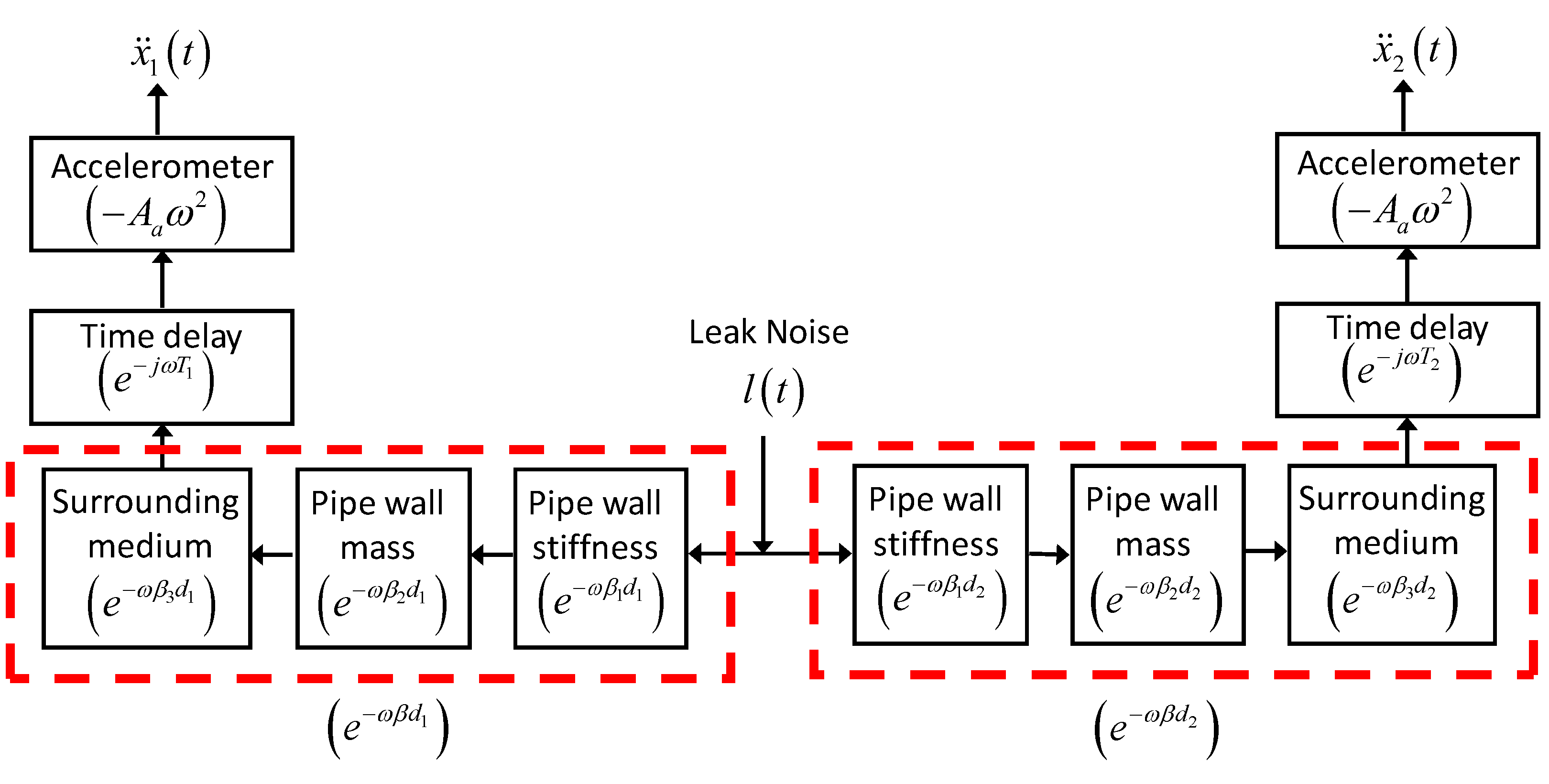
5. Calculating the Frequency Bandwidth of Measured Leak Noise from a Buried Pipe Surrounded by an External Medium

When the inertial effect of the pipe is considered, and/or when the pipe is surrounded by a medium such as water or soil, then β β 0 and c c 0 are frequency dependent. In these cases, Equation (6a,b) are no longer valid and the analysis to determine the frequency range over which measured leak noise occurs is more complicated. This section is devoted to the analysis of the system in the more general case when the pipe is either submerged under water or buried in soil.

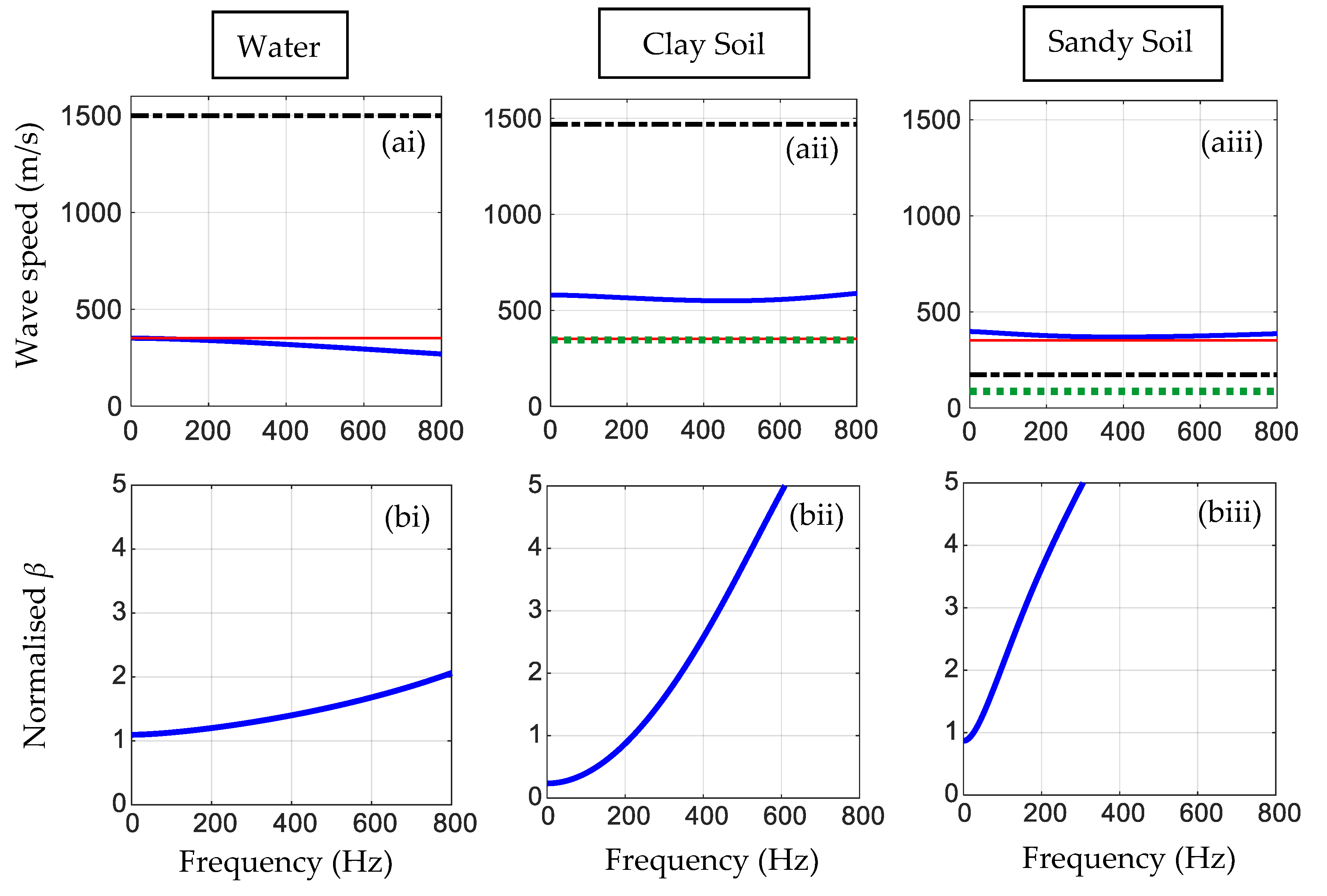
5.1. Wave Speed and Attenuation Factor

Before considering the bandwidth of leak noise when there is a surrounding medium to the pipe, the wave speed in the pipe given by c = ω / Re k and the attenuation factor β = Im k / ω need to be determined. The wavenumber k is a function of the pipe geometry and material, and the properties of the surrounding medium are shown in Appendix A. Using the model for the wavenumber in Appendix A and the properties of the pipe and surrounding medium given in Table 1 and Table 2, the wave speed is plotted in Figure 3(ai–aiii) for systems with an MDPE pipe surrounding by water, clay soil and sandy soil, respectively. Additionally, shown in the graphs are other wave speeds. One is the wave speed for a massless in vacuo pipe given by [10] c 0 c water 1 + K ˜ ( water ) / K ^ ( pipe ) 1 2 , where K ˜ ( water ) = 2 B water / a is the stiffness of the water and K ^ ( pipe ) = E pipe h / a 2 is the hoop stiffness of the pipe. The others correspond to the shear and dilatational wave speeds in the external medium, which are defined in Appendix A.
In the in vacuo case of a massless water-filled pipe, the attenuation factor is given by [10] β 0 η pipe / 2 c 0 1 + K ^ pipe / K ˜ water 1 , where η pipe is the loss factor of the pipe wall. Note that this is a constant; however, as mentioned above, if the surrounding medium and the inertia of the pipe wall are considered, then β is frequency dependent. The actual attenuation factor, normalised by β 0 for the systems with the corresponding wave speeds shown in Figure 3(ai–aiii), are plotted in Figure 3(bi–biii). The specific features of these graphs for a surrounding medium of water [32], clay soil and sandy soil [15,33] are discussed in the following subsubsections. The properties of these test rigs have been determined from measurements at different test sites, for example in [15,33], and are given in Table 1 and Table 2.

5.1.1. Pipe Surrounded by Water

The wave speed is plotted in Figure 3(ai). Additionally plotted is the wave speed for a massless in vacuo pipe for comparison and the speed of the dilatational wave in the surrounding water. The main effect of the pipe mass and the mass-loading effect of the surrounding water is to marginally reduce the wave speed from c 0 as frequency increases. Because the wave speed in the pipe is less than the dilatational wave speed in the surrounding medium, a wave does not propagate from the pipe into the surrounding medium. Thus, the acoustic energy is contained within the pipe. However, because the wave speed and the corresponding wavelength in the pipe reduces with frequency because of mass loading, the attenuation factor β increases with frequency. This can be seen in Figure 3(bi), which is a plot of β / β 0 as a function of frequency. A change in β affects the bandwidth of the measured leak noise, and this is discussed in Section 5.

5.1.2. Pipe Surrounded by Clay Soil

The wave speed is plotted in Figure 3(aii). Additionally plotted is the wave speed for a massless in vacuo pipe for comparison and the wave speeds of the dilatational and shear waves in the surrounding. At zero frequency, the wave speed in the pipe is given by c c water 1 + K ˜ ( water ) / K ^ ( pipe ) 1 ν pipe 2 + 2 G medium / a 1 2 . Note that this is different from that of the in vacuo case, which is given by c c water 1 + K ˜ ( water ) / K ^ ( pipe ) 1 2 . For the parameters given in Table 1 and Table 2, this results in a wave speed of about 585 m/s. It can be seen that as frequency increases, the wave speed first decreases by a small amount, which is predominantly due to the mass loading of the soil, and then increases by a small amount, which is due to radiation into the soil by the shear wave. Note that the dilatational wave does not propagate away from the pipe because its wave speed is greater than the wave speed in the pipe.
The normalised value of β is plotted in Figure 3(bii). It can be seen that this is less than unity at zero frequency, but it increases rapidly with frequency. As the pipe wave speed is approximately constant with frequency, it has a negligible effect on β . The loss of vibrational energy from the pipe to the soil is, thus, the main factor that influences the frequency dependency of β .

5.1.3. Pipe Surrounded by Sandy Soil

The wave speed is plotted in Figure 3(aiii). Additionally plotted is the wave speed for a massless in vacuo pipe for comparison and the wave speeds of the dilatational and shear waves in the surrounding soil. As with the pipe surrounded by clay soil, at zero frequency, the wave speed in the pipe is c c water 1 + K ˜ ( water ) / K ^ ( pipe ) 1 ν pipe 2 + 2 G medium / a 1 2 . For the parameters given in Table 1 and Table 2, this results in a wave speed of about 398 m/s, which remains approximately constant over the whole frequency range shown. This is much lower than for the pipe surrounded by clay soil because sandy soil has a much lower shear modulus. As both the shear and dilatational wave speeds in the soil are smaller than the pipe wave speed, they both propagate into the soil, leaking vibrational energy from the pipe.
The normalised value of β is plotted in Figure 3(biii). It can be seen that this is slightly less than unity at zero frequency, but it increases much more rapidly with frequency than for the pipe surrounded by clay soil. This is because there is an additional wave propagating into the soil, leaking more vibrational energy from the pipe. As the pipe wave speed is approximately constant with frequency, it is the loss of vibrational energy from the pipe to the soil that influences the frequency dependency of β .

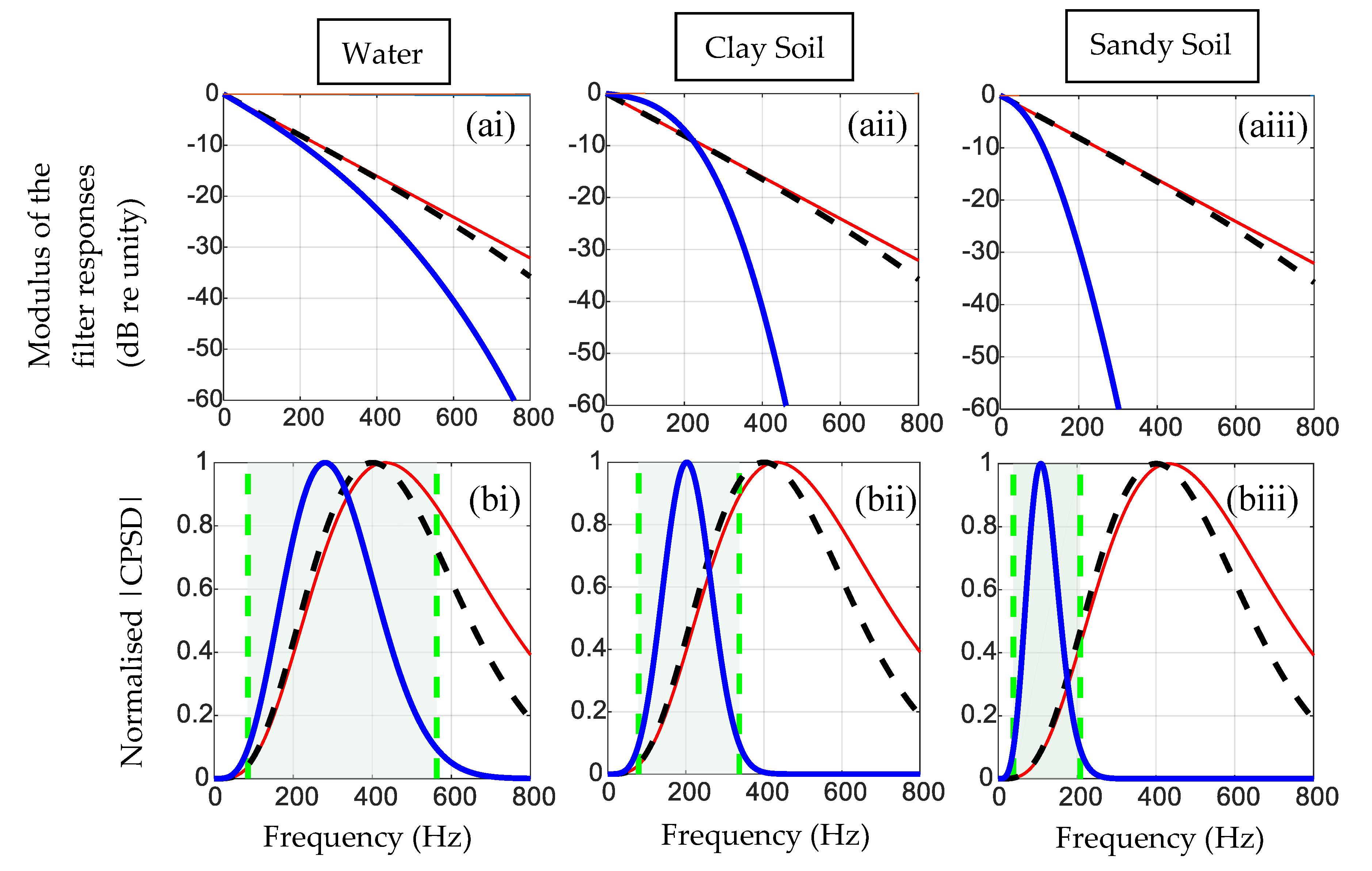
5.2. Factors Affecting the Bandwidth of Measured Leak Noise

Having established the way in which the pipe system parameters affect the propagation of leak noise in terms of the propagation velocity and attenuation, the frequency range of the leak noise is now considered. Figure 4 shows a way of describing each component of the pipe system as a filter; consequently, the whole system becomes a cascade of filters.
As shown in Figure 4, there are three filters modelling the in vacuo pipe without inertial effects, the pipe-wall mass effect, and the surrounding medium, respectively. One filter describes the time delay (from the leak to the sensors’ location) and one filter is related to the transducer’s dynamic behaviour, which is illustrated by using an accelerometer in Figure 4. The filters related to the transducer and those related to both the water-filled pipe and the surrounding medium are the ones affecting the frequency range of measured leak noise. The filtering effects of each component of the system is analysed using the modulus of the CPSD but not including accelerometers. This corresponds to pressure measurements and is denoted by e ω β d , which can be written as e ω β 1 + β 2 + β 3 d or e ω β 1 d e ω β 2 d e ω β 3 d . Figure 5(ai–iii) show the CPSDs for different combinations of filter responses, considering an external medium of water, clay soil and sandy soil, respectively, with d being arbitrarily set to 20 m. One filter is related to the massless in vacuo pipe e ω β 1 d , another one involves the inclusion of inertial effects in the model e ω β 1 + β 2 d , and the third one further includes the external medium e ω β 1 + β 2 + β 3 d . It is important to note that they are plotted on a dB scale so that the low-pass behaviour of each case considered can be distinguished easily. It is quite evident that the surrounding medium is a dominant factor. The system where the pipe is buried in sandy soil, which has the largest value of β . has the most profound effect on the measured leak noise frequency range.
In Section 3, it was shown that for a constant value of β , which is the case for a massless in vacuo water-filled pipe, the modulus of the CPSD has a peak when ω β d = 4 or at a frequency in Hz of f = 2 / π β d for the accelerometer measurements. If β is not a constant, which is the case when inertial effects of the pipe or the surrounding media are considered, it is not possible to determine such a simple closed-form solution. In general, β increases because of the external medium, and hence, its effect is to limit the measured leak noise to lower frequencies. This is seen in Figure 5a. The CPSDs corresponding to those plotted in Figure 5(ai–iii) are combined with the FRFs for the sensors (accelerometers) and are plotted normalised by the maximum value in Figure 5(bi–iii). Additionally, plotted is a shaded region that corresponds to the frequency range where the |CPSD| > one tenth of the maximum peak of the |CPSD|, i.e., where the modulus of the CPSD is within 10 dB of the maximum. This is calculated numerically. It is possible to see a gradual shift to lower frequencies when the inertial effect of the pipe along with the external medium are taken into account. Moreover, when the surrounding medium changes from water to clay and to sandy soil, there is a progressive shifting to lower frequency of the frequency range and a narrowing of the bandwidth.

6. Experimental Work

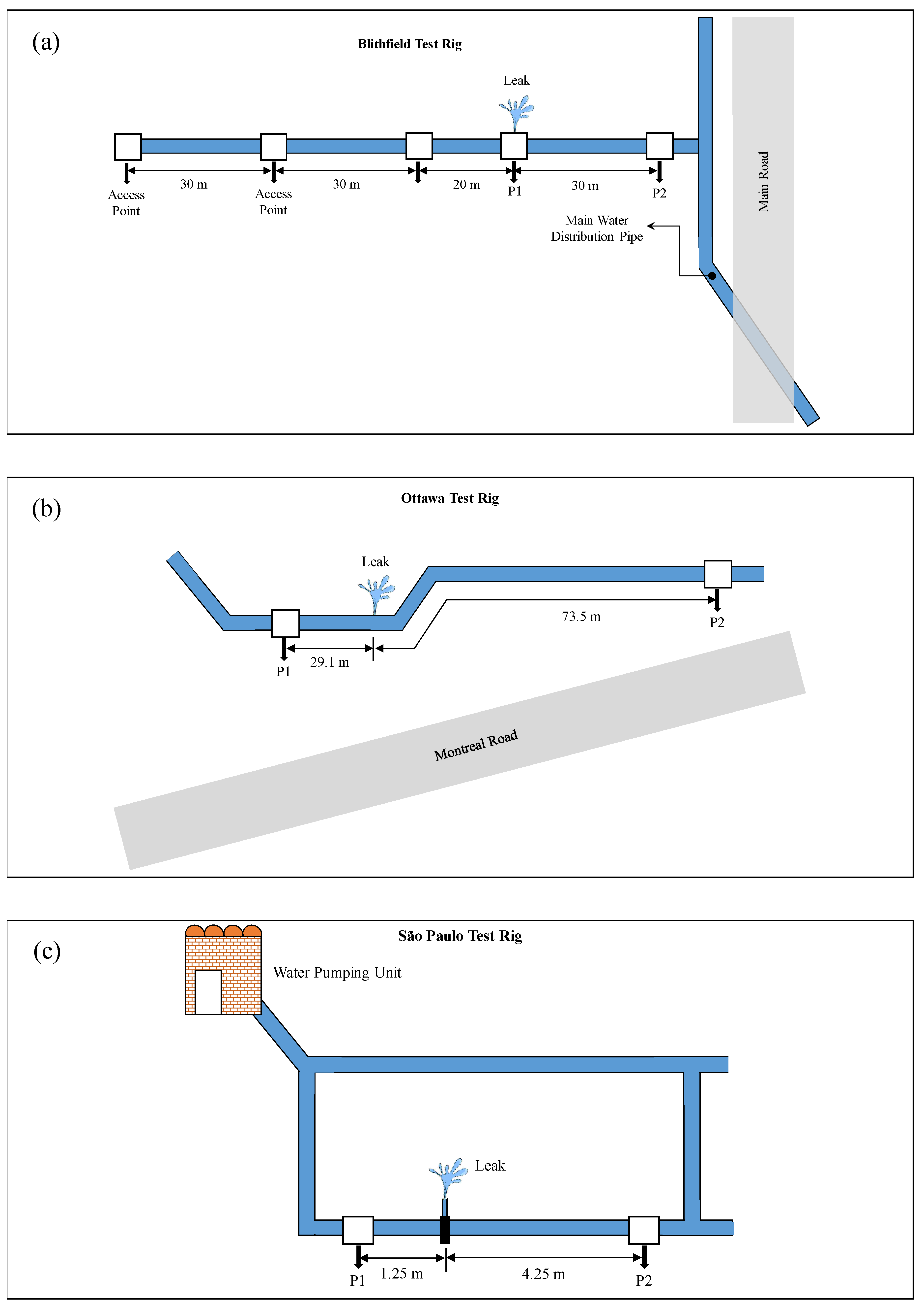
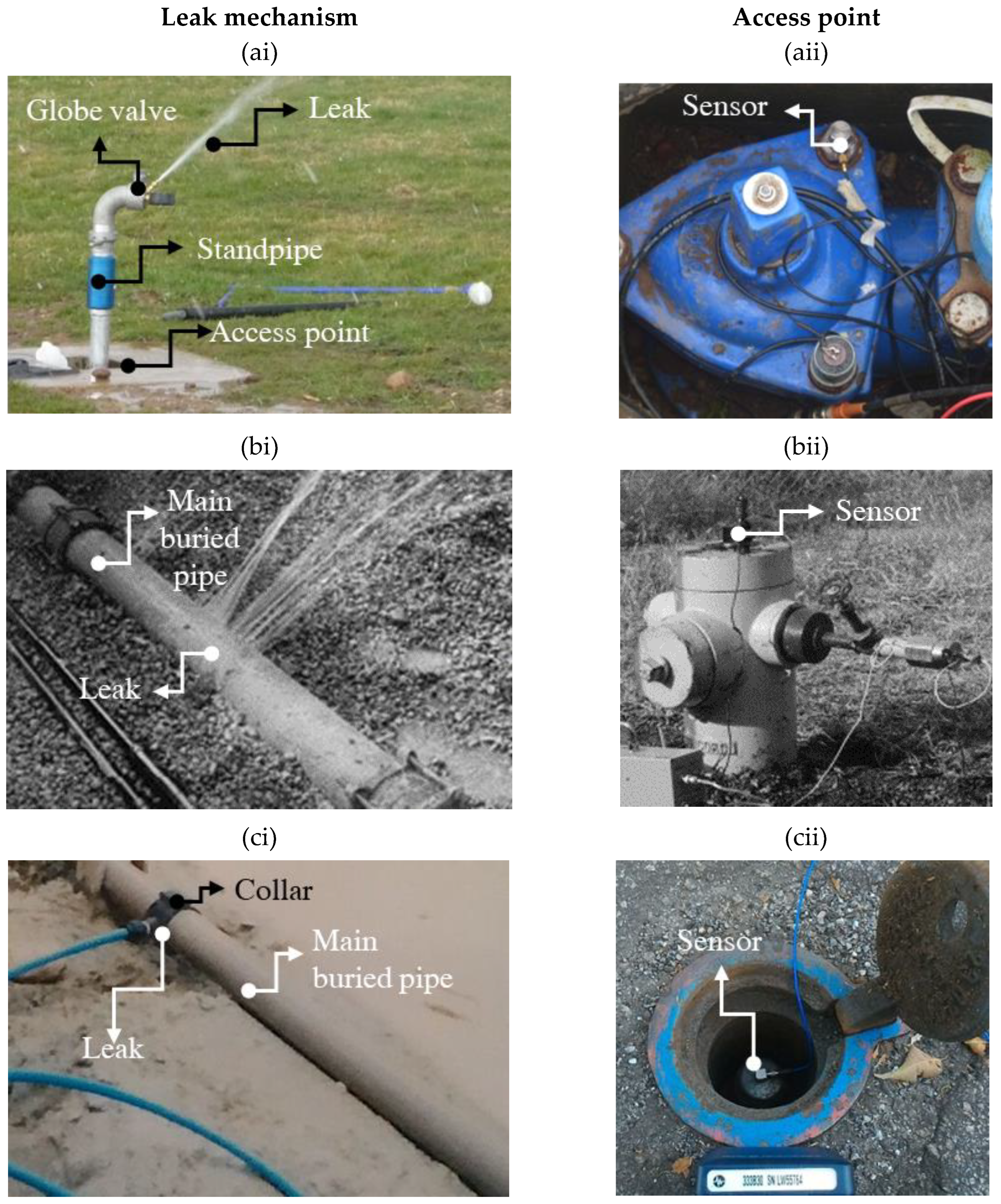
6.1. Descriptions of Test Rigs

To investigate if the method presented in this paper can predict the frequency range of leak noise data, some experimental results are compared with the analytical predictions. Additionally, to evaluate the robustness of the proposed model, data from three very different test rigs are considered. They are located in Blithfield (UK), Ottawa (Canada) and São Paulo (Brazil). Their schematic diagrams are shown in Figure 6a–c, respectively. Details of these test rigs have been reported previously (Blithfield [12], Ottawa [34,35], São Paulo [15,27,33]) and so only important details are given here. Note also, that the way in which the leak was created in the three test rigs is different. In each case, measurements were made using accelerometers, and photographs showing the leaks together with the sensor arrangements is shown in Figure 7a–c). Note that the photographs of the leaks in the Ottawa and São Paulo test rigs show the pipes before they were buried.
The Blithfield test rig is 120 m long, has 5 access points, and is connected to the mains water supply [12]. The pipe is made from high-performance polyethylene (HPPE) and is buried at a depth of about 0.8 m in sandy soil. The estimated pipe and soil properties are given in Table 3 and Table 4 [27]. The measurement positions were at access points P1 and P2 (30 m apart) and the leak was created at point P1, as shown in Figure 6a. The access points are underground metal hydrant valves, which connect the sections of the buried plastic water pipe. The leak was generated using a small globe valve attached to the end of a standpipe connected to the underground hydrant valve, as can be seen in Figure 7(ai), and the vibration of the pipe was measured using type 4383 Bruel and Kjaer accelerometers, one of which can be seen in Figure 7(aii). Two 60-second time histories were recorded using a DATS data acquisition system at a sampling frequency of 5 kHz.
The Ottawa test rig is about 200 m long and consists of a PVC pipe connected to the mains network. It is buried in soft clay soil at a depth of 2.4 m. The estimated pipe and soil properties are given in Table 3 and Table 4. Data from this test rig have been used in several studies, for example [10,27,36,37]. The measurement positions were at access points P1 and P2, which are 102.6 m apart, with the leak located 29.1 m from point P1, as shown in Figure 6b. The access points are above ground and are connected to the buried pipe by risers. The leak was generated by way of a crack in the pipe, as illustrated in Figure 7(bi), and the vibration was measured using accelerometers with a sensitivity of 1 V/g, one of which can be seen in Figure 7(bii). Two 66-second time histories were recorded at a sampling frequency of 500 Hz.
The São Paulo test rig is a small closed-circuit test rig that is separate from the mains water system and pressurised by a centrifugal pump. It consists of a polyvinyl chloride (PVC) pipe buried at a depth of about 0.5 m in stiff clay soil [15,33]. The estimated pipe and soil properties are given in Table 3 and Table 4. The measurement positions were at access points P1 and P2, which are 5.5 m apart, with the leak located 1.25 m from Point P1, as shown in Figure 6c. The leak was generated by way of a small hole in the pipe with the water being led away to a tank using a small diameter pipe, as illustrated in Figure 7(ci), and the vibration of the pipe was measured using type 4506-B-003 Bruel and Kjaer accelerometers, one of which can be seen in Figure 7(cii). Two 60-second time histories were recorded using an LMS Scadas data acquisition system at a sampling frequency of 12.8 kHz.

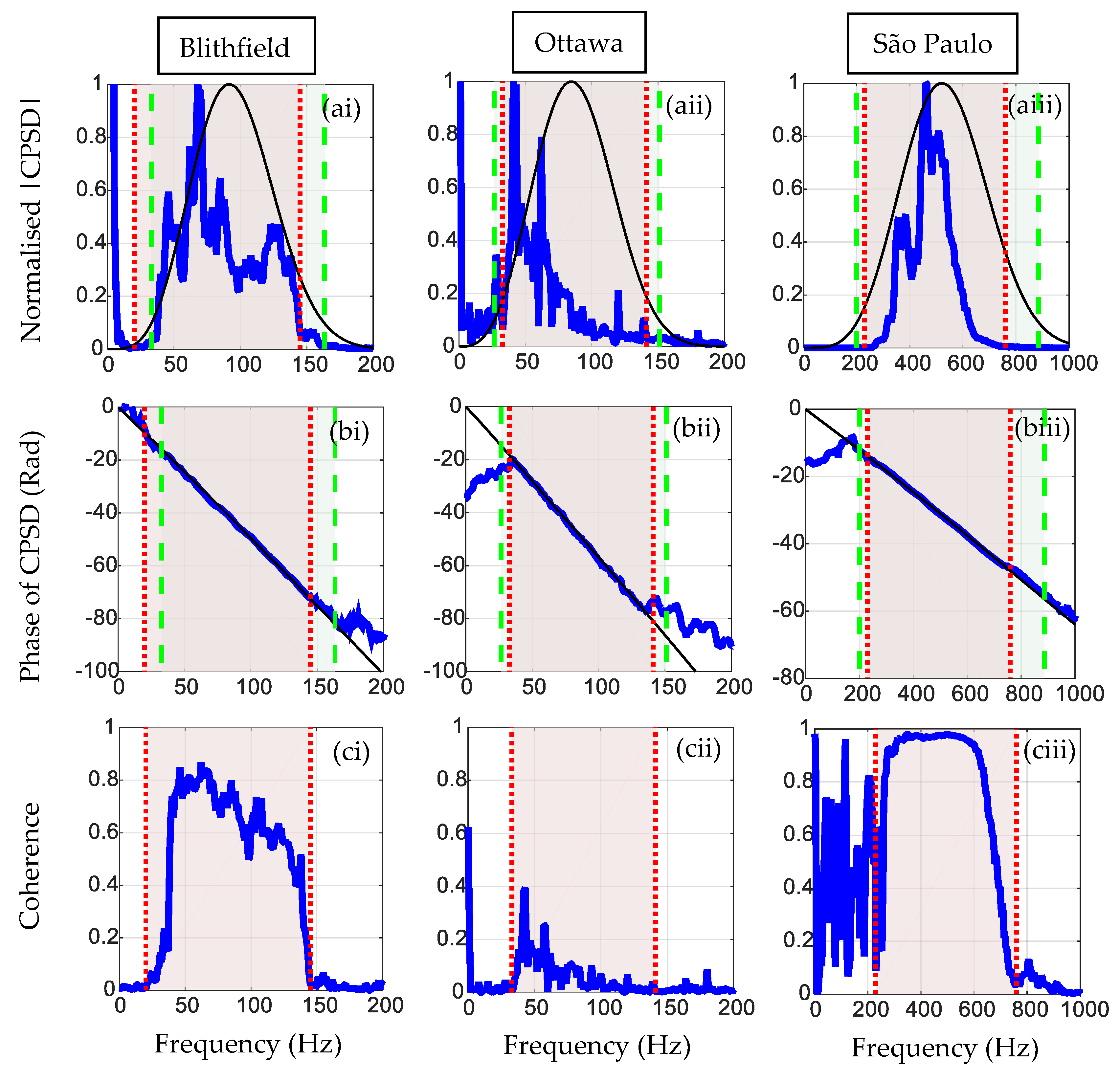
6.2. Experimental Results

Figure 8 shows the experimental results for all three test rigs.
In Figure 8, the graphs depict |CPSD| normalized by its maximum value, the phase of the CPSD and the coherence. The predicted responses for the parameters given in Table 3 and Table 4 are also shown in Figure 8. The experimental measurements have leak noise content within a certain bandwidth because of the band-pass filtering effects of the pipe-surrounding medium-sensor systems and measurement noise [24]. These frequency bands are estimated roughly through the coherence function [37] and are denoted as a shaded area in each case, whose edges are marked with vertical dotted red lines. The predicted leak noise frequency bands, where |CPSD| are within 10 dB of their maximum values, are also plotted as shaded areas, in which the edges are marked with vertical dashed green lines. By examining Figure 8, it can be seen that for all the sites, the model cannot predict the shape of the modulus of the CPSD very well because of measurement noise and unmodelled effects, such as the ground surface, inhomogeneity of the soil, uncertainties from the interface between the pipe and soil, pipe joints and discontinuities, and reflections; however, it does capture the bandwidths, over which there is leak noise, reasonably well, and it is possible to see a similar trend between the experiment and the theory, mainly for Blithfield and São Paulo test rigs. The measured CPSD for the Ottawa test rig does not match very well the theoretical one due to low level of coherence along with the effects mentioned above. Furthermore, note that the model does capture the phase behaviour reasonably well within the frequency ranges where there is leak noise for all the test rigs. The main differences observed in the spectral bandwidth of the São Paulo test rig compared to the other test rigs can be mostly attributed to two factors. Firstly, the pipe geometry of the São Paulo test rig is smaller, as indicated in Table 3. Secondly, the soil in the São Paulo test rig is significantly stiffer, indicated by the values of the bulk and shear moduli, which are much higher compared to the soil in the other test rigs as shown in Table 4. As the distance between the measurement position and the leak increases, the leak noise bandwidth decreases and is restricted to lower frequencies. Attenuation of leak noise, as it propagates in plastic pipes, contributes to this effect. This is highly influenced by the pipe geometry/properties along with the properties of the surrounding medium.

7. Conclusions

This paper has demonstrated the influence of the physical parameters of the pipe-soil–sensor system on the measured leak noise frequency range. The approach involves integrating a compact analytical model of the pipe system with the frequency response of the sensors and a model of the CPSD between the two sensors. The effects of the physical parameters on the CPSD and further on the frequency range of the leak noise for different types of surrounding medium, namely water, stiff clay soil and sandy soil, have been investigated. The surrounding medium has a dominant effect on the bandwidth of the measured leak noise. Moreover, it has been shown that the distance between the sensors together with wave speed of the predominantly fluid wave in the pipe and the attenuation of this wave are the three key factors affecting this range of frequencies. The centre frequency can be impacted by the distance between the sensors, while the upper and lower frequencies are not affected. A low (high) centre frequency is observed when the sensors are placed at a large (small) distance from each other and when the soil has a small (large) shear stiffness. The loss of energy propagating into the surrounding medium as the leak noise wave travels along the pipe has a profound effect on the centre frequency and the upper and lower frequencies of leak noise bandwidth. When a considerable amount of vibrational energy propagates into the surrounding medium, then the centre frequency of the CPSD gets lower, and it reduces the range of frequencies. Experimental data from three different testing sites have successfully validated the method proposed in this paper for predicting the bandwidth of the leak noise. Despite its advantages, this method has some limitations including poor estimation when the level of coherence between the measured signal is low. Other effects such as inhomogeneity of the soil, discontinuities due to pipe connections/joints, reflections can also affect the predictions. Nevertheless, the applicability of the method and its simplicity allow an estimate of the bandwidth of the measured leak noise to be made for a given situation, which is extremely useful when using leak noise correlators to pinpoint a leak.

Author Contributions

Conceptualization, M.J.B.; methodology M.J.B., O.S. and F.C.L.d.A.; software, M.J.B., O.S. and F.C.L.d.A.; validation, O.S.; investigation, M.J.B., O.S. and F.C.L.d.A.; resources M.J.B., F.C.L.d.A. and J.M.M.; data curation, F.C.L.d.A. and J.M.M.; writing—original draft preparation, M.J.B. and O.S.; writing—review and editing, F.C.L.d.A., M.K.I., J.M.M., P.F.J. and Y.G.; visualization, M.J.B., O.S., F.C.L.d.A., M.K.I., J.M.M., P.F.J. and Y.G.; supervision, M.J.B., F.C.L.d.A. and J.M.M.; project administration, M.J.B.; funding acquisition, M.J.B., F.C.L.d.A. and J.M.M. All authors have read and agreed to the published version of the manuscript.

Funding

The authors are grateful for the financial support provided by the São Paulo Research Foundation (FAPESP) under Grant numbers 2018/25360-3 and 2019/00745-2. Oscar Scussel is grateful for the support from Coordination for the Improvement of Higher Education Personnel (CAPES) under Grant number 88887.374001/2019-00 and EPSRC under the project RAINDROP (EP/V028111/1).

Data Availability Statement

The data presented in this study are available upon request from the corresponding author.

Acknowledgments

The authors thank the Brazilian water and waste management company (Sabesp) for partly funding this work and for providing one of the test rigs.

Conflicts of Interest

The authors declare no conflict of interest.

Appendix A

This appendix describes an analytical model of a submerged/buried plastic water pipe. A schematic diagram of the pipe system, which includes the pipe wall, the water in the pipe and the surrounding medium, is shown in Figure A1. It has a mean radius a and a wall thickness h.
Figure A1. A water-filled submerged/buried plastic pipe.
Acoustics 05 00029 g0a1
In the derivation of the analytical model the following simplifying assumptions are made:
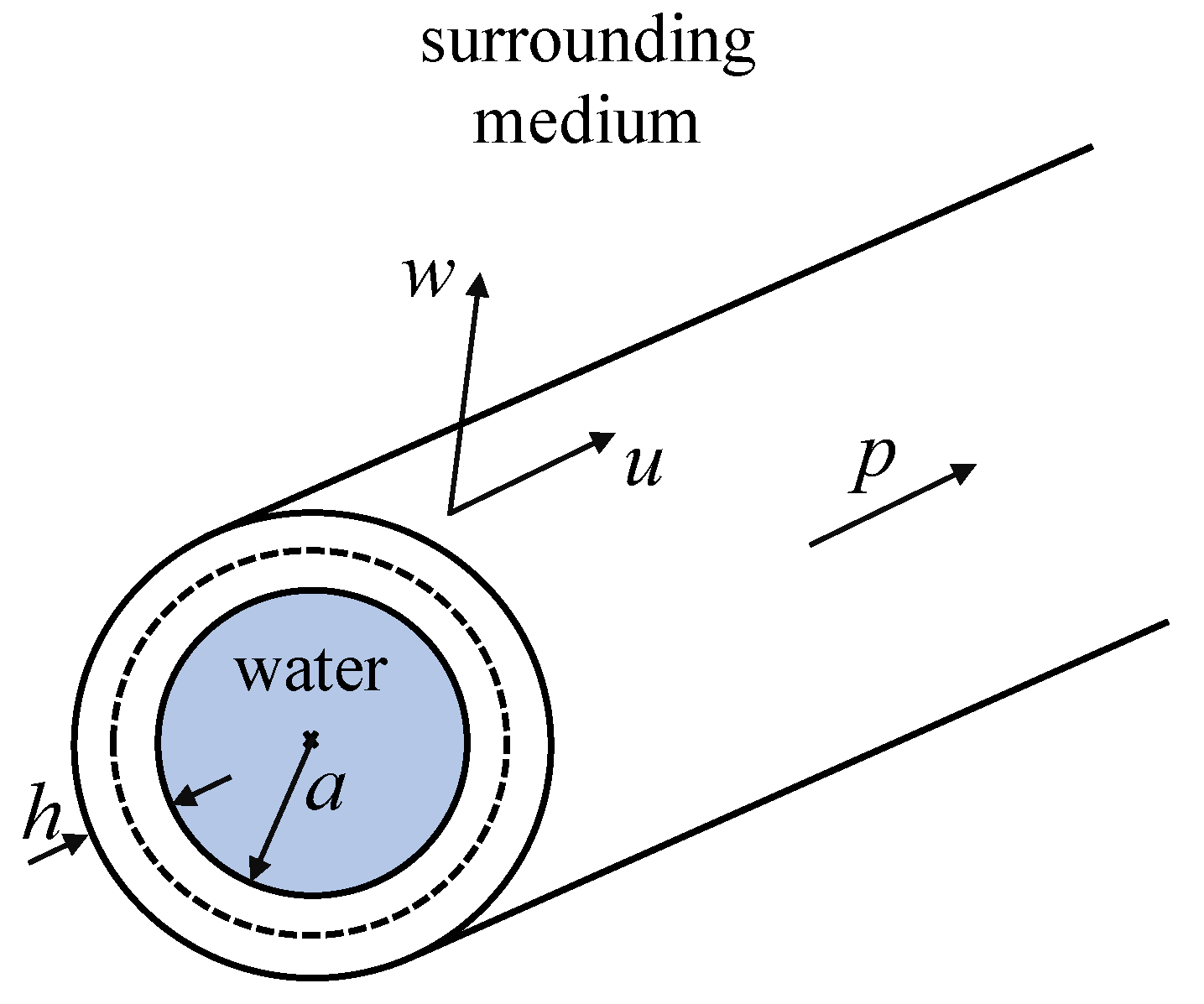
  • The pipe and surrounding medium are of infinite extent in the axial direction, and the surrounding medium is of infinite extent in the radial direction;
  • The predominantly fluid-borne axis-symmetric wave is the only wave propagating in the pipe and is responsible for the propagation of leak noise;
  • The frequency range of interest is well below the pipe-ring frequency so that bending in the pipe wall is neglected;
  • The frequency range of interest is such that an acoustic wavelength of water is much greater than the diameter of the pipe.
The analytical model, which is based on that described by Gao et al. [14], uses the concept of wave dynamic stiffness. This is similar in concept to wave impedance described by Fahy and Gardonio [38], but rather than using the variables of force (or pressure) and velocity, displacement is used instead of velocity as this is more convenient. It essentially involves a pressure that is harmonic in both space and time being applied to a structure or a fluid such that p = P e j ω t k x , where ω is the circular frequency and k is the wavenumber. As the structure or fluid is assumed to be linear, the response is given by w = W e j ω t k x . The wave dynamic stiffness is defined as the ratio P ω , k / W ω , k , i.e., it is a complex quantity that is dependent on both frequency and the wavenumber. The real part of the wave dynamic stiffness is related to the stiffness or inertial properties of the system, and the imaginary part of the wave dynamic stiffness is related to energy dissipation. Here, the wavenumber is written in terms of the wave dynamic stiffness of the component parts of the system, i.e., the water in the pipe, the pipe wall and the surrounding medium. This enables the behaviour of the predominantly fluid-borne wave in a buried plastic water pipe to be interpreted in a physical rather than a mathematical sense. The wavenumber derivation in terms of the wave dynamic stiffness of the component parts of the system starts from the frequency domain equations that govern the axial and radial motion of the pipe wall, which are given by [14]
Ω 2 k a 2 S L 11 j ν pipe k a S L 12 j ν pipe k a S L 21 1 Ω 2 F L S L 22 U W = 0 ,
where Ω = k L a , in which a is the mean radius of the pipe and k L = ω ρ pipe 1 ν pipe 2 / E pipe is the compressional wavenumber of the pipe wall, in which E pipe , ρ pipe ,   and   ν pipe are the Young’s modulus, density and Poisson’s ratio of the pipe wall, respectively; F L and S L i j (i and j = 1, 2) are the fluid and the soil loading terms, respectively. Equation (A1) can be written alternatively as
K ( pipe ) + K ( water ) + K ( medium ) u = 0 ,
where K ( pipe ) is the wave dynamic stiffness matrix for the pipe wall given by,
K ( pipe ) = K 11 ( pipe ) K 12 ( pipe ) K 21 ( pipe ) K 22 ( pipe ) = k a 2 K ˜ ( pipe ) ω 2 ρ pipe h j ν pipe k a K ˜ ( pipe ) j ν pipe k a K ˜ ( pipe ) K ˜ ( pipe ) ω 2 ρ pipe h ,
in which K ˜ ( pipe ) = E pipe * h / a 2 1 ν pipe 2 is the hoop stiffness of a cylindrical ring of unit length, in which the displacement in the axial direction is constrained to be zero; E pipe * = E pipe 1 + j η pipe where η pipe is the material loss factor of the pipe wall. If the speed of a compressional wave in the pipe wall is much greater than the predominantly fluid-borne wave in the pipe (which is the case for plastic water distribution pipes where the wave speed in the pipe wall is typically between 3 and 4 times that of the predominantly fluid-borne wave [25]), such that k a 2 K ˜ ( pipe ) > > ω 2 ρ pipe h , then
K ( pipe ) = K 11 ( pipe ) K 12 ( pipe ) K 21 ( pipe ) K 22 ( pipe ) k a 2 K ˜ ( pipe ) j ν pipe k a K ˜ ( pipe ) j ν pipe k a K ˜ ( pipe ) K ˜ ( pipe ) ω 2 ρ pipe h ,
The wave dynamic stiffness matrix for the water contained in the pipe is given by
K ( water ) = 0 0 0 K ( water ) = [ 0 0 0 ω 2 ρ water k water R J 0 k water R a J 0 k water R a ] ,
where J 0 is a Bessel function of the first kind of zero order, and k water R = k water 2 k 2 is the component of the wavenumber in the radial direction, in which k water = ω / c water is the wavenumber for water, and where c water is the wave speed in an infinite homogeneous body of water, which is approximately 1500 m/s. At low frequencies, when the acoustic wavelength in water is much greater than the diameter of the pipe J 0 k water R a / J 0 k water R a 2 / k water R a . Additionally, noting that k water 2 = ω 2 ρ water / B water , Equation (A4a) can be written as
K ( water ) = 0 0 0 K ( water ) 0 0 0 K ˜ ( water ) / 1 k 2 k water 2 ,
where K ˜ ( water ) = 2 B water / a , in which B water is the bulk modulus of water.
The wave dynamic stiffness matrix for the surrounding medium is given by
K ( medium ) = K 11 ( medium ) K 12 ( medium ) K 21 ( medium ) K 22 ( medium ) = G medium α k d R j 2 α H ¯ d k j 2 α H ¯ d k 2 a + α H ¯ s H ¯ d k s R ,
where H 0 is a Hankel function of the second kind of zero order, k s R = k s 2 k 2 , in which k s = ω / c s is the shear wavenumber for the surrounding medium, and k d R = k d 2 k 2 , in which k d = ω / c d is the dilatational wavenumber for the surrounding medium, where c d = B medium + 4 G medium / 3 / ρ medium and c s = G medium / ρ medium are the wave speeds corresponding to dilatational and shear waves, respectively, in which B medium , G medium and ρ medium are the bulk modulus, shear modulus and density of the surrounding medium, respectively; H ¯ s = H 0 k s R a / H 0 k s R a , H ¯ d = H 0 k d R a / H 0 k d R a , and α = k s 2 / k d R k s R H ¯ s + k 2 H ¯ d .
If the surrounding medium is water, it has no shear stiffness, and Equation (A5) becomes
K ( medium ) = K 11 ( medium ) K 12 ( medium ) K 21 ( medium ) K 22 ( medium ) = 0 0 0 B water k d 2 k d R H ¯ d ,
Note that K 21 ( pipe ) = K 12 ( pipe ) and K 21 ( soil ) = K 12 ( soil ) . The second row of the matrix equation in Equation (A1) can be rearranged to give an expression for the wavenumber in terms of the wave dynamic stiffnesses of the pipe, the surrounding medium and the soil to give
k = k water 1 + K ˜ ( water ) K ( pipe ) + K ( pipe _ medium ) + K ( medium ) 1 2 ,
where K ( pipe ) = K 22 ( pipe ) , K ( pipe _ medium ) = K 12 ( pipe ) + K 12 ( medium ) 2 / K 11 ( pipe ) + K 11 ( medium ) and K ( medium ) = K 22 ( medium ) . Note that the wavenumber is a function of the wave dynamic stiffnesses. One of these is related to the water in the pipe K ˜ ( water ) , one to the pipe alone K ( pipe ) , one to the surrounding medium alone K ( medium ) , and one that is related to the interaction between the surrounding medium and the pipe K ( pipe _ medium ) . Note, however, that the wave dynamic stiffnesses in Equation (A7) are functions of k, so Equation (A7) must be solved recursively [26]. If there is no axial distributed force acting on the pipe from the surrounding medium, as would be the case if the surrounding medium is water, then K ( pipe _ medium ) = 0 . This boundary condition was considered by Muggleton and Yan [13] in the case when the surrounding medium is soil. Formulating the wavenumber in terms of the wave dynamic stiffnesses of the components of the pipe system facilitates an investigation into the way in which the pipe properties and the interface between the soil and the pipe affects the wave behaviour in terms of the wave speed and wave attenuation.

References

  1. United States Environmental Protection Agency Report, Water Audits and Water Loss Control for Public Water Systems. 2013. Available online: https://www.epa.gov/sites/default/files/2015-04/documents/epa816f13002.pdf (accessed on 3 March 2023).
  2. EurEau Report, Europe’s Water in Figures. 2017. Available online: https://www.eureau.org/resources/publications/eureau-publications/5824-europe-s-water-in-figures-2021/file (accessed on 3 March 2023).
  3. Globo Report. 2019. Available online: https://g1.globo.com/economia/noticia/2019/06/05/oito-estados-do-pais-perdem-metade-ou-mais-da-agua-que-produzem-com-vazamentos-e-gatos-diz-estudo.ghtml (accessed on 3 March 2023).
  4. BBC Report. 2014. Available online: https://www.bbc.com/news/world-latin-america-29947965 (accessed on 3 March 2023).
  5. National Geographic Report. 2018. Available online: https://www.nationalgeographic.com/news/2018/02/cape-town-running-out-of-water-drought-taps-shutoff-other-cities/ (accessed on 3 March 2023).
  6. BBC Report. 2019. Available online: https://www.bbc.com/news/world-asia-india-49232374 (accessed on 3 March 2023).
  7. UKWIR Reports. 2017. Available online: https://www.ukwir.org/How-will-we-achieve-zero-leakage-in-a-sustainable-way-by-2050 (accessed on 3 March 2023).
  8. Puust, R.; Kapelan, Z.; Savic, D.A.; Koppel, T. A review of methods for leakage management in pipe networks. Urban Water J. 2010, 7, 25–45. [Google Scholar] [CrossRef]
  9. Fuchs, H.V.; Riehle, R. Ten years of experience with leak detection by acoustic signal analysis. Appl. Acoust. 1991, 33, 1–19. [Google Scholar] [CrossRef]
  10. Gao, Y.; Brennan, M.J.; Joseph, P.F.; Muggleton, J.M.; Hunaidi, O. A model of the correlation function of leak noise in buried plastic pipes. J. Sound Vib. 2004, 277, 133–148. [Google Scholar] [CrossRef]
  11. Gao, Y.; Brennan, M.J.; Joseph, P.F.; Muggleton, J.M.; Hunaidi, O. On the selection of acoustic/vibration sensors for leak detection in plastic water pipes. J. Sound Vib. 2005, 283, 927–941. [Google Scholar] [CrossRef]
  12. Almeida, F.C.L.; Brennan, M.J.; Joseph, P.F.; Whitfield, S.; Dray, S.; Paschoalini, A.T. On the acoustic filtering of the pipe and sensor in a buried plastic water pipe and its effect on leak detection: An experimental investigation. Sensors 2014, 14, 5595–5610. [Google Scholar] [CrossRef] [PubMed]
  13. Muggleton, J.M.; Yan, J. Wavenumber prediction and measurement of axisymmetric waves in buried fluid-filled pipes: Inclusion of shear coupling at a lubricated pipe/soil interface. J. Sound Vib. 2013, 332, 1216–1230. [Google Scholar] [CrossRef]
  14. Gao, Y.; Sui, F.; Muggleton, J.M.; Yang, J. Simplified dispersion relationships for fluid-dominated axisymmetric wave motion in buried fluid-filled pipes. J. Sound Vib. 2016, 375, 386–402. [Google Scholar] [CrossRef]
  15. Brennan, M.J.; Karimi, M.; Muggleton, J.M.; Almeida, F.C.L.; de Lima, F.K.; Ayala, P.C.; Obata, D.; Paschoalini, A.T.; Kessissoglou, N. On the effects of soil properties on leak noise propagation in plastic water distribution pipes. J. Sound Vib. 2018, 427, 120–133. [Google Scholar] [CrossRef]
  16. Xu, W.; Fan, S.; Wang, C.; Wu, J.; Yao, Y.; Wu, J. Leakage identification in water pipes using explainable ensemble tree model of vibration signals. Measurement 2022, 194, 110996. [Google Scholar] [CrossRef]
  17. Fares, A.; Tijani, I.A.; Rui, Z.; Zayed, T. Leak detection in real water distribution networks based on acoustic emission and machine learning. Environ. Technol. 2022, 15, 1–17. [Google Scholar] [CrossRef]
  18. Cheng, W.; Shen, Y. Frequency Characteristic Analysis of Acoustic Emission Signals of Pipeline Leakage. Water 2022, 14, 3992. [Google Scholar] [CrossRef]
  19. Sitaropoulos, K.; Salamone, S.; Sela, L. Frequency-based leak signature investigation using acoustic sensors in urban water distribution networks. Adv. Eng. Inform. 2023, 55, 101905. [Google Scholar] [CrossRef]
  20. Han, X.; Cao, W.; Cui, X.; Gao, Y.; Liu, F. Plastic Pipeline Leak Localization Based on Wavelet Packet Decomposition and Higher Order Cumulants. IEEE Trans. Instrum. Meas. 2022, 71, 3520911. [Google Scholar] [CrossRef]
  21. Xu, T.; Zeng, Z.; Huang, X.; Li, J.; Feng, H. Pipeline leak detection based on variational mode decomposition and support vector machine using an interior spherical detector. Process Saf. Environ. Prot. 2021, 153, 167–177. [Google Scholar] [CrossRef]
  22. Diao, X.; Jiang, J.; Shen, G.; Chi, Z.; Wang, Z.; Ni, L.; Mebarki, A.; Bian, H.; Hao, Y. An improved variational mode decomposition method based on particle swarm optimization for leak detection of liquid pipelines. Mech. Syst. Signal Process. 2020, 143, 106787. [Google Scholar] [CrossRef]
  23. Chew, A.W.Z.; Kalfarisi, R.; Meng, X.; Pok, J.; Wu, Z.Y.; Cai, J. Acoustic feature-based leakage event detection in near real-time for large-scale water distribution networks. J. Hydroinform. 2023, 25, 526–551. [Google Scholar] [CrossRef]
  24. Scussel, O.; Brennan, M.J.; Almeida, F.C.L.; Iwanaga, M.K.; Muggleton, J.M.; Joseph, P.F.; Gao, Y. An Investigation into the Factors Affecting the Bandwidth of Measured Leak Noise in Buried Plastic Water Pipes. In Recent Trends in Wave Mechanics and Vibrations; Dimitrovová, Z., Biswas, P., Gonçalves, R., Silva, T., Eds.; Springer: Cham, Switzerland, 2023; Volume 125, pp. 1031–1038. [Google Scholar] [CrossRef]
  25. Pinnington, R.J.; Briscoe, A.R. Externally applied sensor for axisymmetric waves in a fluid filled pipe. J. Sound Vib. 1994, 173, 503–516. [Google Scholar] [CrossRef]
  26. Muggleton, J.M.; Brennan, M.J.; Linford, P.W. Axisymmetric wave propagation in fluid-filled pipes: Wavenumber measurements in in vacuo and buried pipes. J. Sound Vib. 2004, 270, 171–190. [Google Scholar] [CrossRef]
  27. Scussel, O.; Brennan, M.J.; Almeida, F.C.L.; Muggleton, J.M.; Rustighi, E.; Joseph, P.F. Estimating the spectrum of leak noise in buried plastic water distribution pipes using acoustic or vibration measurements remote from the leak. Mech. Syst. Signal Process. 2021, 147, 107059. [Google Scholar] [CrossRef]
  28. Brennan, M.J.; de Lima, F.K.; Almeida, F.C.L.; Joseph, P.F.; Paschoalini, A.T. A virtual pipe rig for testing acoustic leak detection correlators: Proof of concept. Appl. Acoust. 2016, 102, 137–145. [Google Scholar] [CrossRef]
  29. Gray, J.J.; Tilling, L. Johann Heinrich Lambert, mathematician and scientist, 1728–1777. Hist. Math. 1978, 5, 13–41. [Google Scholar] [CrossRef]
  30. Dence, T.P. A Brief Look into the Lambert W Function. Appl. Math. 2013, 4, 887–892. [Google Scholar] [CrossRef]
  31. Hayes, B. Why W? Am. Sci. 2005, 93, 104–108. Available online: https://www.americanscientist.org/sites/americanscientist.org/files/2005216151419_306.pdf (accessed on 1 March 2023). [CrossRef]
  32. Muggleton, J.M.; Brennan, M.J. Leak noise propagation and attenuation in submerged plastic water pipes. J. Sound Vib. 2004, 278, 527–537. [Google Scholar] [CrossRef]
  33. Scussel, O.; Brennan, M.J.; Muggleton, J.M.; Almeida, F.C.L.; Paschoalini, A.T. Estimation of the bulk and shear moduli of soil surrounding a plastic water pipe using measurements of the predominantly fluid wave in the pipe. J. Appl. Geophy. 2019, 164, 237–246. [Google Scholar] [CrossRef]
  34. Hunaidi, O.; Chu, W.T. Acoustical characteristics of leak signals in plastic water distribution pipes. Appl. Acoust. 1999, 58, 235–254. [Google Scholar] [CrossRef]
  35. Hunaidi, O.; Chu, W.; Wang, A.; Guan, W. Detecting leaks in plastic pipes. J. Am. Water Works Assoc. 2000, 92, 82–94. [Google Scholar] [CrossRef]
  36. Gao, Y.; Brennan, M.J.; Liu, Y.; Almeida, F.C.L.; Joseph, P.F. Improving the shape of the cross-correlation function for leak detection in a plastic water distribution pipe using acoustic signals. Appl. Acoust. 2017, 127, 24–33. [Google Scholar] [CrossRef]
  37. Almeida, F.C.L.; Brennan, M.J.; Joseph, P.F.; Gao, Y.; Paschoalani, A.T. The effects of resonances on time delay estimation for water leak detection in plastic pipes. J. Sound Vib. 2018, 420, 315–329. [Google Scholar] [CrossRef]
  38. Fahy, F.; Gardonio, P. Sound and Structural Vibration: Radiation, Transmission and Response, 2nd ed.; Elsevier: Oxford, UK, 2007. [Google Scholar]
Figure 1. Schematic of leak noise propagation measurement in a buried plastic water pipe using vibration signals and a correlator.
Acoustics 05 00029 g001
Figure 2. Normalised modulus of the CPSD for a massless in vacuo water-filled pipe. Acceleration data, (thick blue line); velocity data, (thin red line). The modulus of the CPSD has a peak when ω ^ = 2 and ω ^ = 4 for velocity and acceleration data, respectively. The circles and the squares indicate the limits of the bandwidth for a 10 dB drop from the maximum peak for velocity and acceleration data, respectively.
Acoustics 05 00029 g002
Figure 3. Properties of three systems with same buried MDPE pipe for a surrounding medium of (i) water, (ii), clay soil, and (iii) sandy soil; (a) wave speeds; pipe surrounded by the medium, (thick blue solid line); massless in vacuo pipe (thin red solid line); shear wave in the external medium (thick green dotted line); dilatational wave in the external medium, (thick black dashed-dotted line). (b) Normalised value of β .
Acoustics 05 00029 g003
Figure 4. Schematic of the water-pipe system represented as a set of filters.
Acoustics 05 00029 g004
Figure 5. Analysis of the water-pipe system behaviour described in terms of filters, with sensors 20 m apart. (a) Modulus of the filter response of the in vacuo pipe with no inertial effects, (thin solid line); modulus of the response of the in vacuo pipe with mass, (thick dashed line); modulus of the response of the pipe taking into account the surrounding medium, (thick solid line). (b) modulus of the CPSDs corresponding to the systems in (a), including accelerometers at each measurement position. (i) Water, (ii) Clay soil and (iii) Sandy Soil. The shaded region bounded by vertical dashed green line is the frequency range for the full system (pipe, surrounding medium, accelerometers) where the modulus of the CPSD is within 10 dB of the maximum.
Acoustics 05 00029 g005
Figure 6. Schematic diagrams of the test rigs for leak measurements, highlighting the measurement and leak positions, and main features. The diagrams are not to scale. (a) Blithfield test rig in the UK, (b) Ottawa test rig in Canada, (c) São Paulo test rig in Brazil.
Acoustics 05 00029 g006
Figure 7. Photographs of the leak mechanism, instrumentation and measurement positions corresponding to the test rigs shown in Figure 6. (a) Blithfield test rig in the UK, (b) Ottawa test rig in Canada, (c) São Paulo test rig in Brazil. (i) Leak mechanism, (ii) Access point.
Acoustics 05 00029 g007
Figure 8. Comparison of measurements carried out in the three experimental rigs and predictions made using the proposed model with the parameters given in Table 3 and Table 4. (a) |CPSD|, (b) phase of the CPSD, (c) coherence; experimental results (thick solid blue lines); predictions (thin solid black lines). The shaded region bounded by the thick dotted red lines denotes the bandwidth where there is good coherence; the shaded area bounded by the thick dashed green lines denotes the frequency range predicted by the model. (i) Blithfield, (ii) Ottawa and (iii) São Paulo.
Acoustics 05 00029 g008
Table 1. MDPE pipe properties used in the simulations.
Properties of the MDPE PipeValue
Young’s modulus E pipe (N/m2) 2 × 10 9
Density ρ pipe (kg/m3)900
Loss factor η pipe 0.06
Poisson’s ratio ν pipe 0.4
Pipe mean radius a (mm)84.5
Pipe-wall thickness h (mm)11
Table 2. Water and soil properties used in the simulations.
PropertiesWaterStiff Clay SoilSandy Soil
Bulk   modulus   B water ,   B medium (N/m2) 2.25 × 10 9 4.0 × 10 9 4.0 × 10 7
Shear   modulus   G medium (N/m2)0 2.4 × 10 8 1.5 × 10 7
Bulk and shear loss factor000
Density   ρ medium (kg/m3)100020002000
Poisson’s ratio0.50.470.33
Dilatational   wave   speed   c d (m/s)15001414141
Shear   wave   speed   c s (m/s)034686
Table 3. Properties of the pipes in the experimental test rigs.
Properties of the PipeBlithfieldOttawaSão Paulo
Young’s modulus E pipe (N/m2) 1.78 × 10 9 4.18 × 10 9 4.3 × 10 9
Density ρ pipe (kg/m3)900900900
Loss factor η pipe 0.060.040.06
Poisson’s ratio ν pipe 0.40.40.4
Pipe radius a (mm)807535.8
Pipe-wall thickness h (mm)9.859.853.4
Table 4. Water and soil properties of the experimental test rigs.
PropertiesBlithfieldOttawaSão Paulo
Bulk   modulus   B medium (N/m2) 1.36 × 10 8 4.0 × 10 8 4.0 × 10 9
Shear   modulus   G medium (N/m2) 3.2 × 10 7 1.0 × 10 5 1.44 × 10 8
Bulk and shear loss factor0.0600
Density   ρ medium (kg/m3)200020002000
Poisson’s ratio0.390.50.49
Dilatational   wave speed   c d (m/s)2994471442
Shear   wave speed   c s (m/s)1267552
Disclaimer/Publisher’s Note: The statements, opinions and data contained in all publications are solely those of the individual author(s) and contributor(s) and not of MDPI and/or the editor(s). MDPI and/or the editor(s) disclaim responsibility for any injury to people or property resulting from any ideas, methods, instructions or products referred to in the content.

