Article

Acoustic Radiation of a Beam Subjected to Transverse Load

Department of Engineering Mechanics, Faculty of Engineering, University of Rijeka, 51000 Rijeka, Croatia
*
Author to whom correspondence should be addressed.
Acoustics 2023, 5(2), 462-475; https://doi.org/10.3390/acoustics5020027
Submission received: 3 February 2023 / Revised: 11 March 2023 / Accepted: 27 April 2023 / Published: 5 May 2023

Abstract

:
In this paper, the dynamic response of a Euler–Bernoulli beam subjected to transverse harmonic forces is calculated. The method of separation of variables combined with the mode shape superposition method, which includes the determination of eigenvalues, is used to define the velocity field of the beam surface. The Rayleigh integral was used to calculate the sound radiation and the beam was placed in an infinite baffle. Additional actuators are introduced in order to minimize the sound radiation, or, more specifically, the total sound power level of the vibrating beam, and their optimal position and force amplitude are determined; the conclusions were drawn from the optimization results. This paper proposes a method for faster determination of the optimal actuator parameters in order to achieve the minimum total sound power level. The validity of the obtained results is demonstrated with examples, whose solutions are compared to the results in the published literature.

1. Introduction

Sound radiation around vibrating flat components is of practical importance and has been intensively researched for many years. With the development of the industry, the flat structural elements used are becoming larger and more flexible, while their natural frequencies and damping are relatively low. Due to the increasing requirements for reducing the vibrations of such elements (e.g., in aircraft), the application of active control is occupying an increasingly important place [1]. Smart materials, such as piezoelectric actuators, are often used as sensors and actuators to control their vibrations [2].
The calculation of sound radiation is based on placing a vibrating flat source in an infinite baffle and calculating the sound field using an integral approach [3,4], usually by one of the following methods: integration of the sound intensity on the hemisphere in the far field, or integration of the sound intensity on the surface of the vibrating flat source.
In this paper, the solutions of both approaches are compared for the parametric testing of the acoustic properties of vibrating beams.
To simulate the vibrations of a flat construction element, a beam of constant rectangular cross-section was chosen, with simple supports attached to its ends.
This paper uses the Euler–Bernoulli theory to define the kinematics of the beam and the mode superposition method. In cases where the structure vibrates simultaneously with multiple vibration modes, each individual vibration mode contributes to the total sound radiation of the structure. If the material damping is neglected, the vibration modes are real, but in case of higher damping or if the complexity of the modes is too large, the acoustic radiation must be investigated on the basis of complex modes [5]. Moreover, the sound radiation of each vibration mode is not independent, and the coupling between them affects the total sound power. It is shown in the literature [6] that the effects of modal coupling are negligible for a structure with resonant excitation and/or high excitation frequency. However, for lowfrequency excitation and non-resonant excitation, the contributions of modal coupling can be significant. Modal radiation efficiencies were also studied by the authors of [7]. The results show that without considering the effects of the cross-modal coupling, the radiated sound power can be well over- or -underestimated even at resonance frequencies. Thus, it is difficult to determine when the modal interaction can be neglected, but in the literature, the modal interaction is often omitted in order to simplify the calculation of the sound power [8].
The Rayleigh integral was used to calculate the sound radiation. It should be noted that the Rayleigh integral is valid only for plate-like structures. However, it is possible to replace the acoustic model with a more advanced model for more complex structures, such as a boundary element model [9,10,11].
The vibration response of the beam was calculated for the excitation and actuator action perpendicular to the beam (along the vertical axis) and at specific positions on the beam. In this paper, an analysis of the influence of the actuator parameters on the total sound power level was performed and the optimal solution for the position and amplitude of the actuator force with the minimal total sound power was determined. The same optimization objective was chosen in [12]. In [13], a method is described to find the optimal force driver array (actuators) that allows for the control of all bending modes of the plate within a certain frequency band. In [14], a method for generating a directional sound field by controlling the structural vibration of a plate through multiple actuators is proposed. In [15], a method for optimizing the arrangement of actuators for more effective active noise barriers is described.
Since most of the vibrational energy is accounted for by the forced frequencies near the natural frequencies, the optimal solution was determined using analytical expressions for the sound power of individual vibrational modes and finally confirmed via calculation from the response for the entire frequency range. An efficient method for determining the minimum sound power using the additional actuators was found. The contribution lies in the simplicity of the new method for the determination of the optimal position and amplitude of the actuators, which enables faster determination of the optimal actuator parameters. The final optimal position is confirmed with the simulation of the entire given frequency spectrum.

2. Mathematical Model

The derivation of sound radiation around a vibrating beam involves the evaluation of vibrations and the calculation of sound radiation.
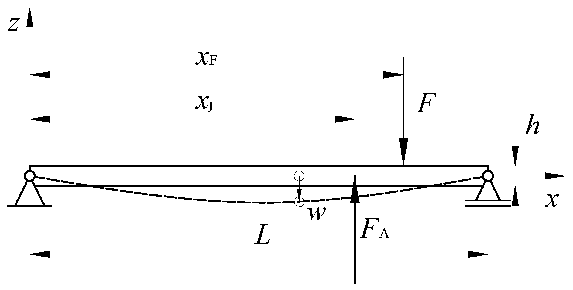
The mathematical model of vibrations of an elastic beam (Figure 1) is represented by differential equations based on the Euler–Bernoulli theory as follows [16,17,18]:
E I 4 u x , t x 4 + ρ s S 2 u x , t t 2 = F x , t
where E is Young’s modulus of elasticity, I is the axial moment of inertia of the cross-section S about the y-axis, u(x,t) is the transverse displacement of the beam, x is the longitudinal axis of the beam, t is the time, ρs is the density of the beam material, and F(x,t) is the load per unit length of the beam. The beam damping is neglected for simplicity.
For forced harmonic oscillations, the displacement of the beam is defined by the expression using the method of separation of variables (Fourier method) as follows:
u x , t = u x e i ω t
where u(x) are the amplitudes of the transverse displacements along the length of the beam and ω is the circular frequency of the harmonic excitation u(x).
The displacement amplitudes, u(x), are obtained using the mode superposition method. This solution is valid for lightly damped (damping ratio ζ < 0.01) [3], harmonically excited flat constructions and it can be used to estimate the response at any excitation frequency. A harmonic excitation F(x,t) of the following form is assumed as:
F x , t = F x e i ω t
The displacement amplitudes along the length of the beam can be determined using the following equation:
d 2 u x d x 2 k f 4 u x = F x E I
where
k f 4 = ω 2 ρ s S E I
The load per unit length of the beam F is defined in [16], as follows:
F x = F F e i φ F δ x x F + j = 1 M F j e i φ j δ x x j
where FF, φF, and xF, and Fj, φj, and xj are the amplitude, phase, and position of the force and actuator, respectively, M is the total number of actuators, and δ(x) is the Dirac function.
The differential Equation (4) is solved for simple supports at the ends of the beam as follows:
u(x) = 0 and My(x) = 0 on x = 0 and x = L
where My is the moment of force about the y-axis, and the natural frequencies and natural modes are defined using the following expressions:
ω n = I E ρ s S n π L 2
u n x = A s i n n π x L
where A is the amplitude and n is the ordinal number of the mode shape.
The general solution of Equation (4) and the chosen boundary conditions of Equation (7) can be obtained using the mode superposition method as follows [16]
u x = 2 ρ s S L n = 1 s i n n π x L ω 2 ω n 2 F F e i φ F s i n n π x F L + j = 1 M F j e i φ j s i n n π x j L
where M is the total number of used actuators.
In practice, the first four mode shapes have the greatest influence on the total level of sound power [19], which is also applied in this paper.
The harmonic waves in the ambient air are defined using the following Helmholtz equation:
p + k 2 p = 0
where p is the acoustic pressure and k is the wave number in the air.
For the interaction between the vibrating surface of the beam and the air surrounding the beam, the following condition,
p z = ρ ω 2 u x
must be fulfilled on the surface of the beam, and the condition,
p z = 0 z = 0
must be fulfilled on the surrounding baffle.
The solution of the Helmholtz equation is the expression for the acoustic pressure, Rayleigh integral [3], as follows:
p x , y , 0 = ρ ω 2 2 π 0 L 0 b e i k r r u x o d x 0 d y 0
where b is the width of the beam, ρ is the air density, and r is the distance between the differential surface dA(x0, y0), and the position (x, y, z = 0) of the sound pressure estimate is as follows:
r = x x 0 2 + y y 0 2
The velocity of the vibrating beam at position x is determined using the following equation:
v x = i ω u x
while the sound power of the vibrating beam is determined using the following:
W ω = 1 2 R e 0 L 0 b p x , y , 0 v * x d x d y
where v* is the conjugate complex velocity.
Since the results of the integrals just described can be obtained only by numerical integration, the calculation was carried out for confirmation with another basic principle, namely, with the sound pressures in the far field [20], as follows:
p f f = i k ρ c e i k r 2 π r 0 b 0 L v x e i α x L + β x b d x d y
where the quantities α and β are defined by the following expressions:
α = k L s i n θ c o s φ
β = k b s i n θ s i n φ
and the quantities φ and θ are the coordinates of the spherical coordinate system (φ, π/2 − θ, r) of which the origin lies in the corner of the beam.
The following is an expression for the sound power based on acoustic pressures on a hemisphere in the far field:
W ω = 0 2 π 0 π 2 p f f 2 ρ c r 2 s i n θ d θ d φ
From the sound power in paper [20], the sound radiation efficiency of an Sn beam vibrating in one of its mode shapes was calculated as follows:
S n = 32 k 2 b L n 2 π 4 0 π 2 0 π 2 c o s s i n α 2 s i n β 2 1 α n π 2 β 2 s i n θ d θ d φ
The cosine function is used when n is an odd integer, while the sine function is used when n is an even integer. From the sound radiation efficiency, the sound power level is calculated according to the following expression:
W n ω = S n ω ρ c b L v ω 2
where v ω 2 is the average mean square surface velocity of the beam surface.
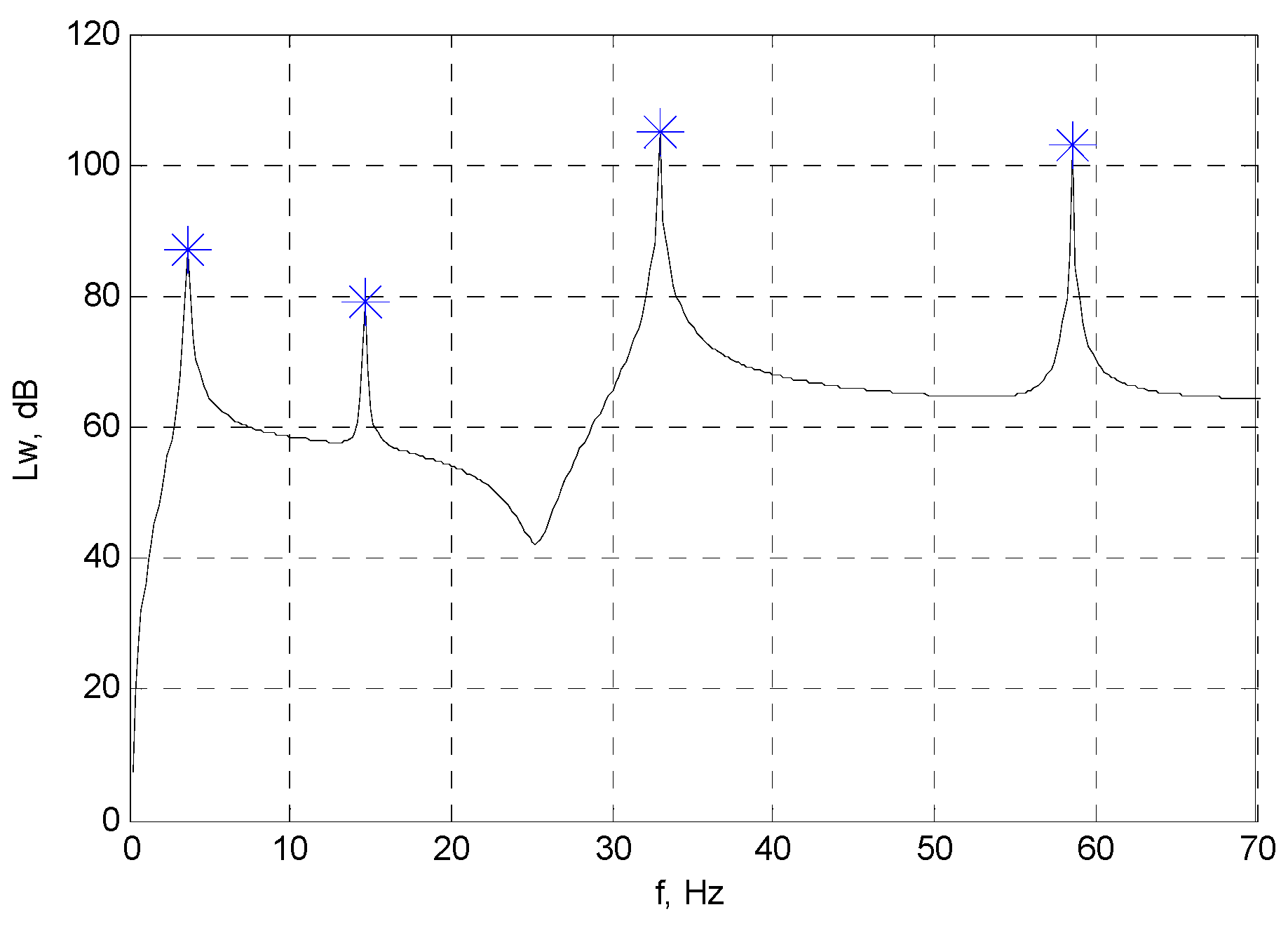
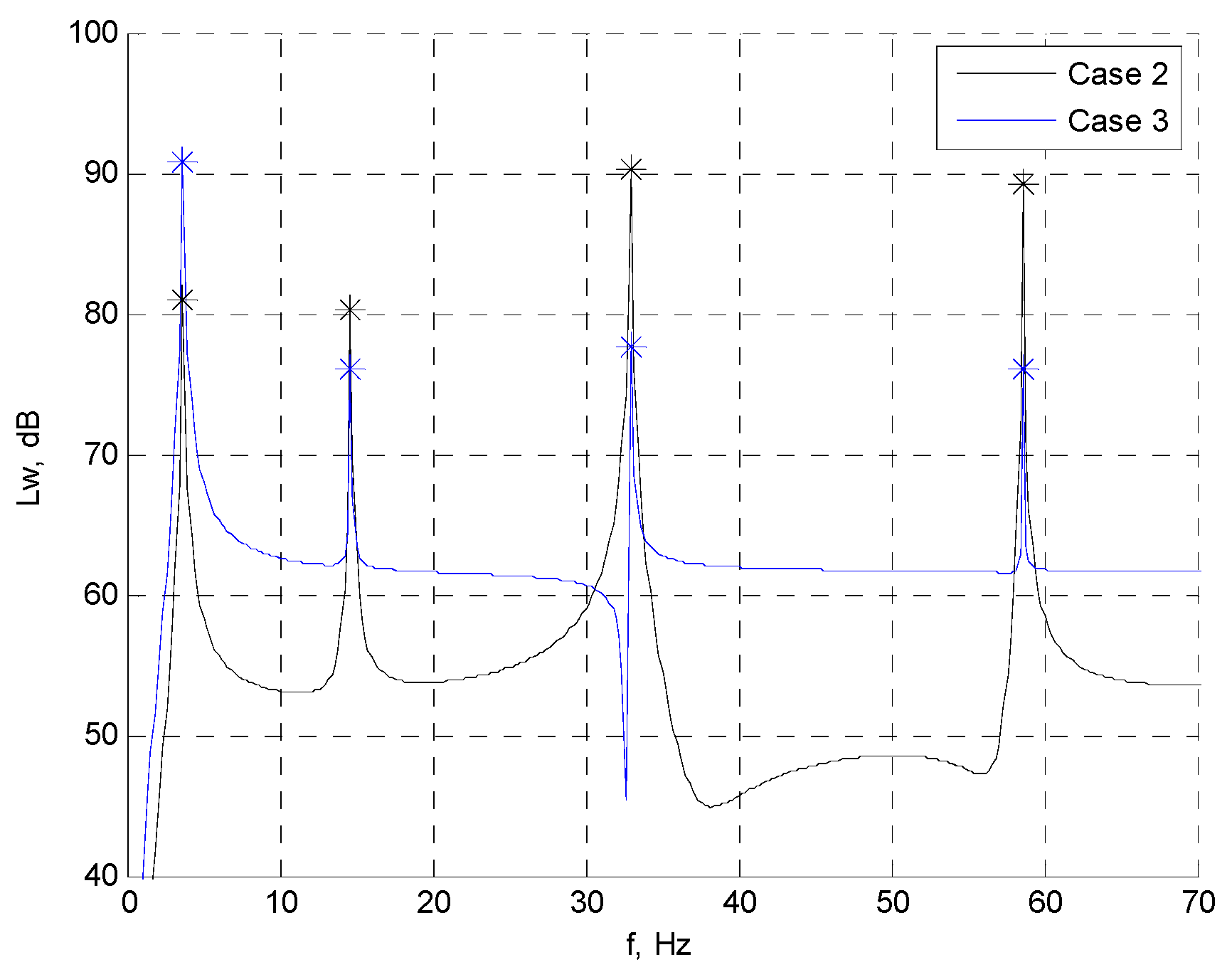
The sound power values calculated according to this procedure are marked with an asterisk in Example 1, and a complete agreement with the numerical result can be seen.
The average mean square surface velocity is calculated using the following expression:
v ω 2 = 1 b L 0 b 0 L 1 2 v 2 d x d y
and for the mode shape of a beam that is simply supported at both ends, the average mean-square surface velocity can be determined using the following expression:
v ω 2 = 1 4 v m 2
where vm is the amplitude of the vibration velocity of the given mode shape.
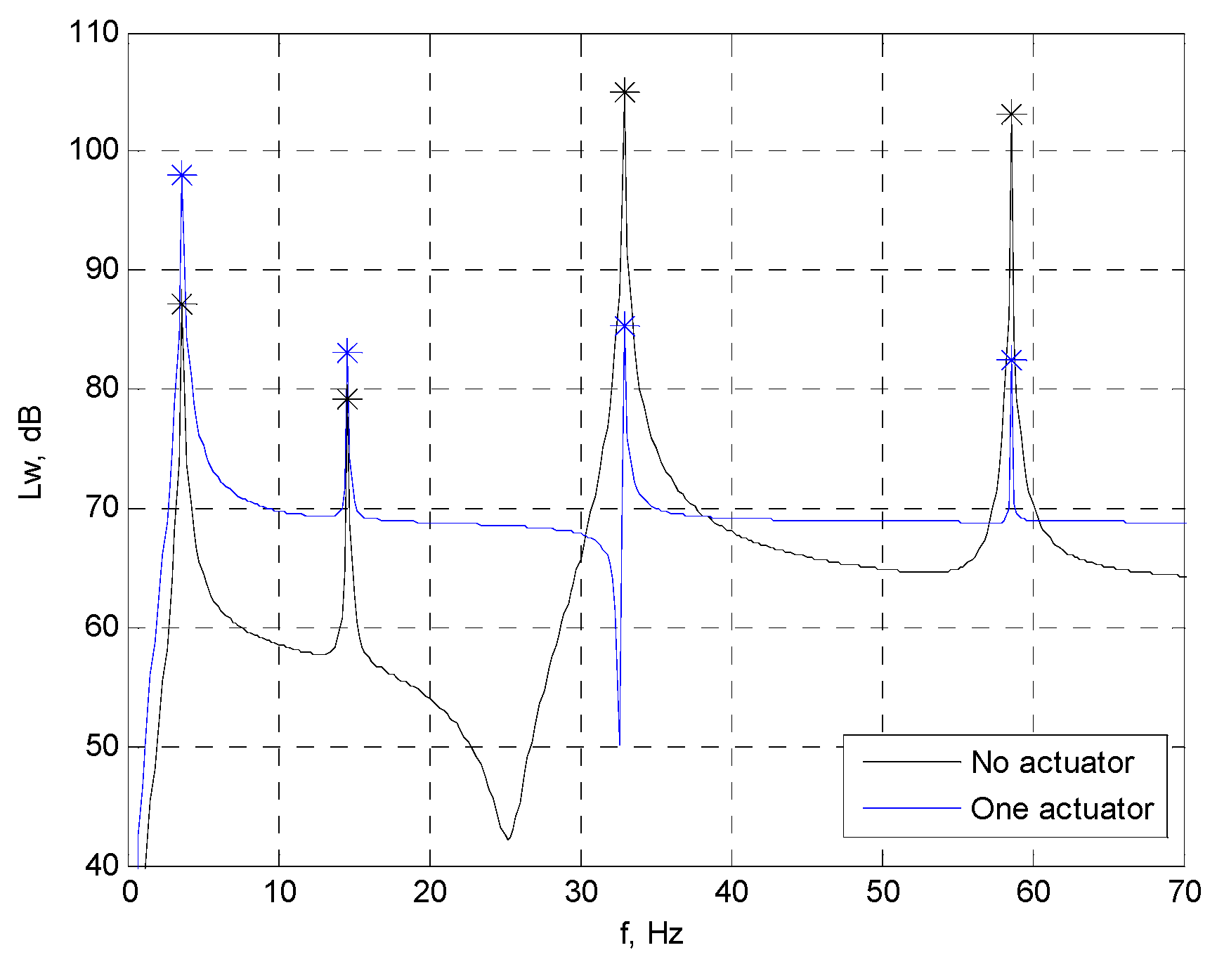
The total response of the beam to the force is determined by the mode superposition method, i.e., for each forced frequency, the response is the sum of its own mode shapes multiplied by the corresponding time functions. If the forced frequency is close to the natural frequency, the beam is assumed to vibrate approximately in the corresponding mode shape. Possible deviations from this were checked by comparing the amplitudes of the excited mode shapes (Example 1).
The sound power level of the beam for the forced circular frequency ω is calculated according to the following expression:
L W = 10 l o g W W 0
where the reference sound power is W0 = 10−12 W.
The total sound power level of the whole spectrum LWtot is calculated by the following expression:
L W t o t = 10 l o g i = 1 N 10 L W i 10
where LWi is the sound power level calculated for a forced circular frequency ω and N is the total number of calculation frequencies or the ratio between the width of the frequency band and the frequency step. The interaction between the vibrational modes is neglected for simplicity. The influence of the parameters (amplitude of the force and position of the force on the total sound power level is considered for a given frequency band. The aim is to determine the minimum total sound power level.
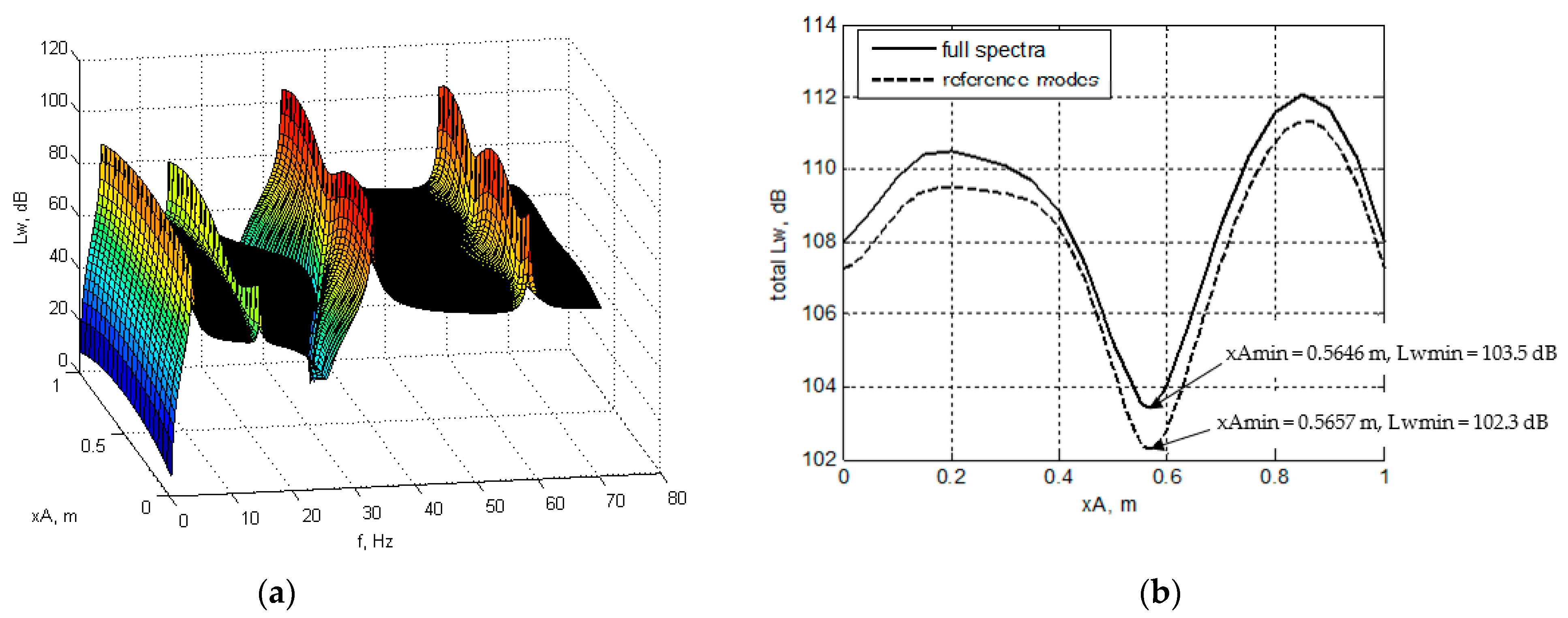
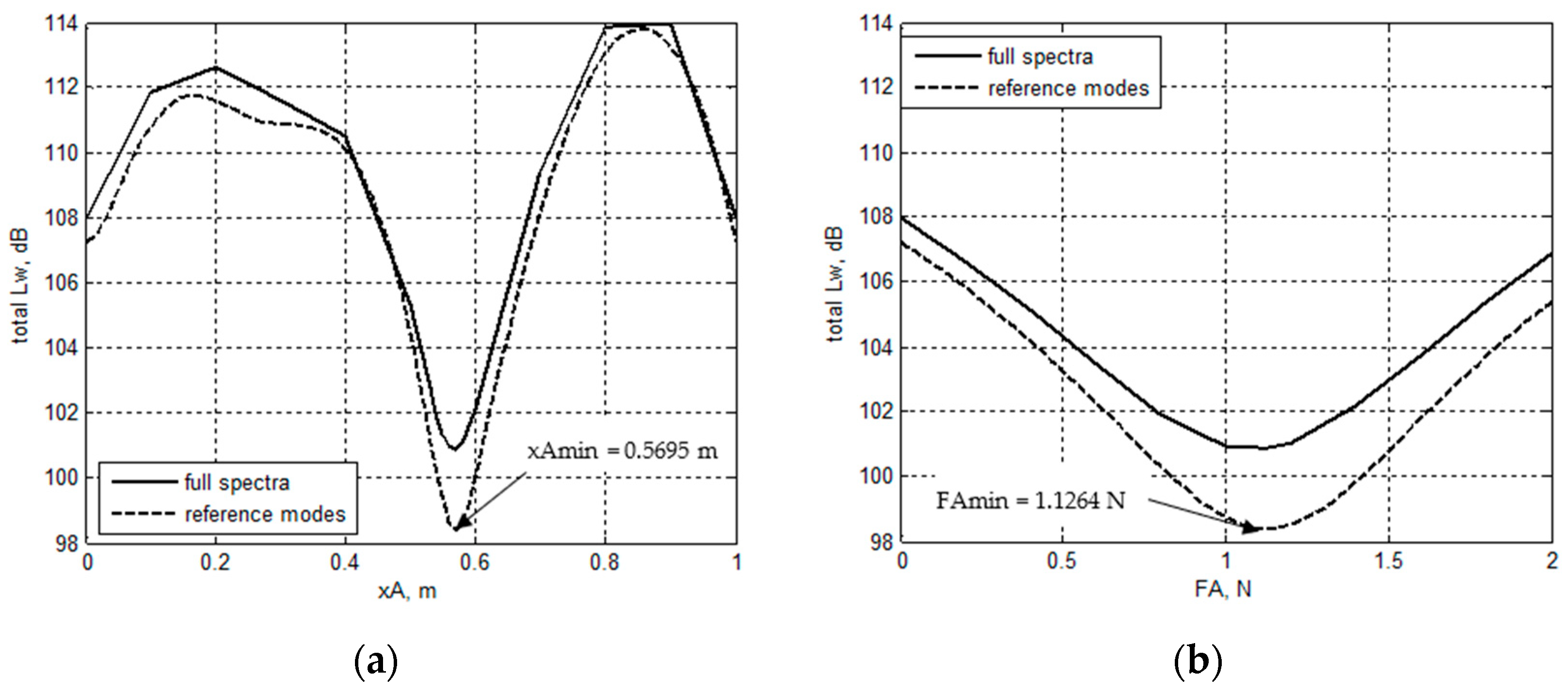
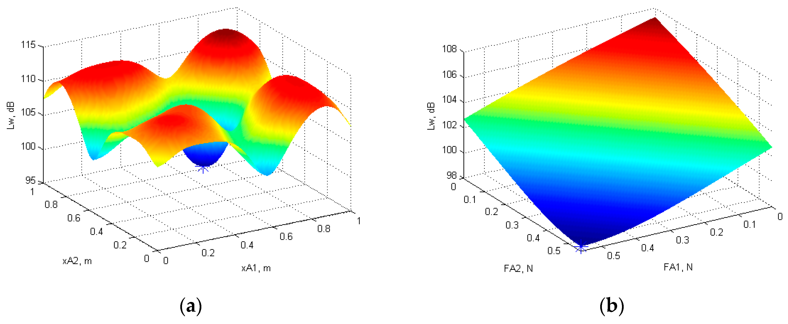
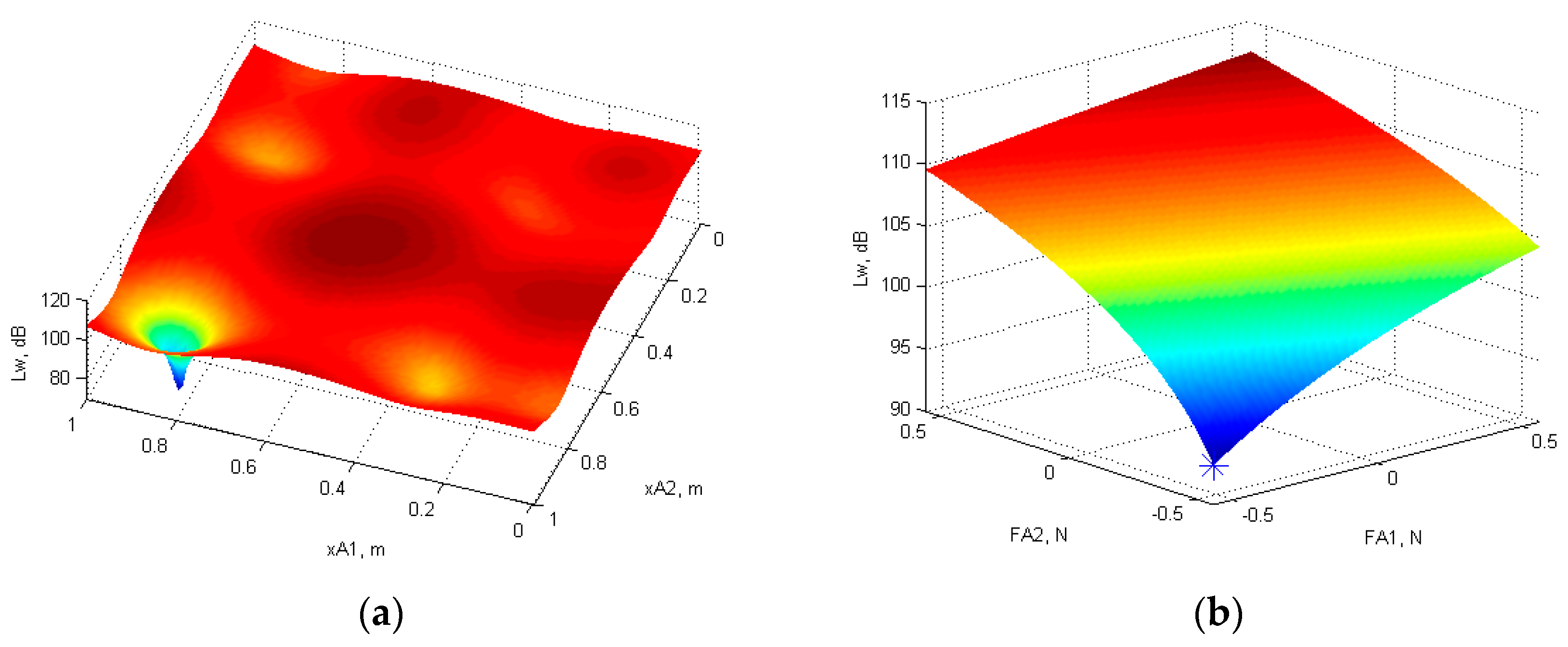
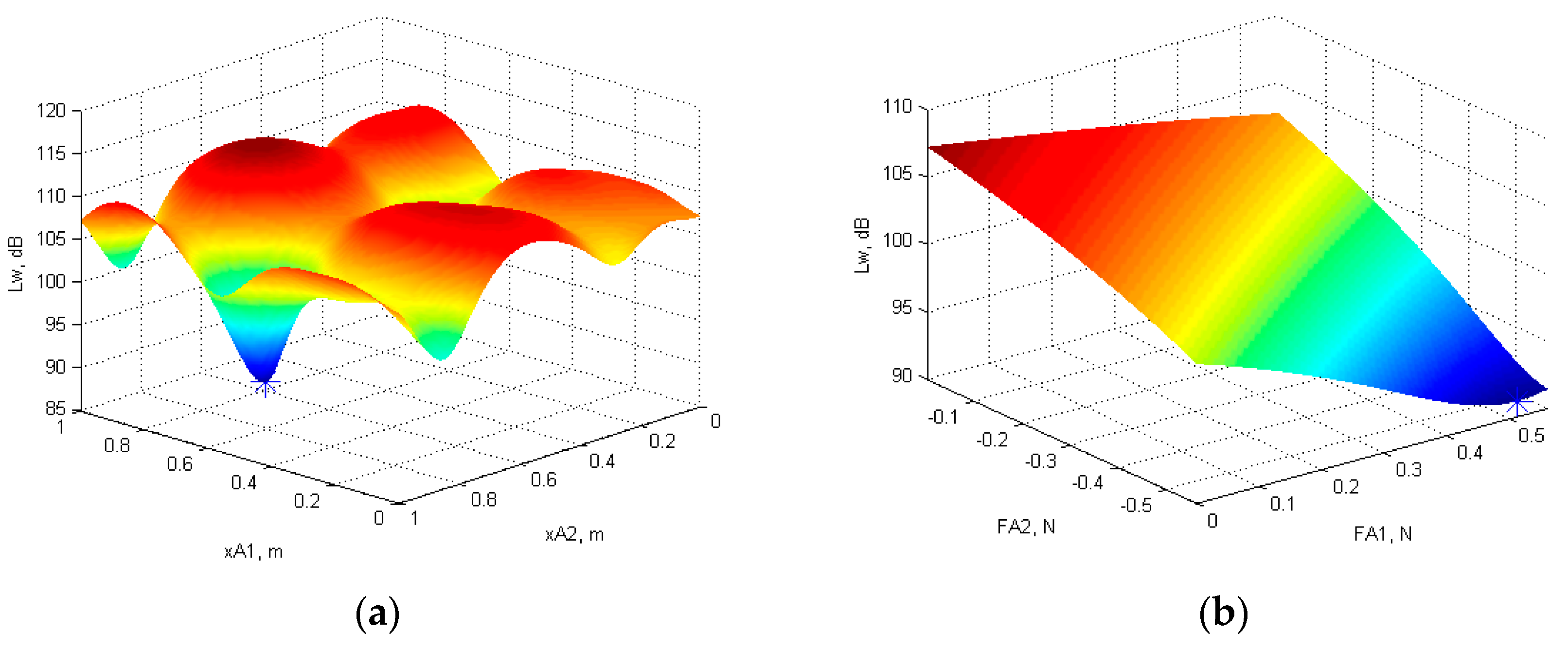
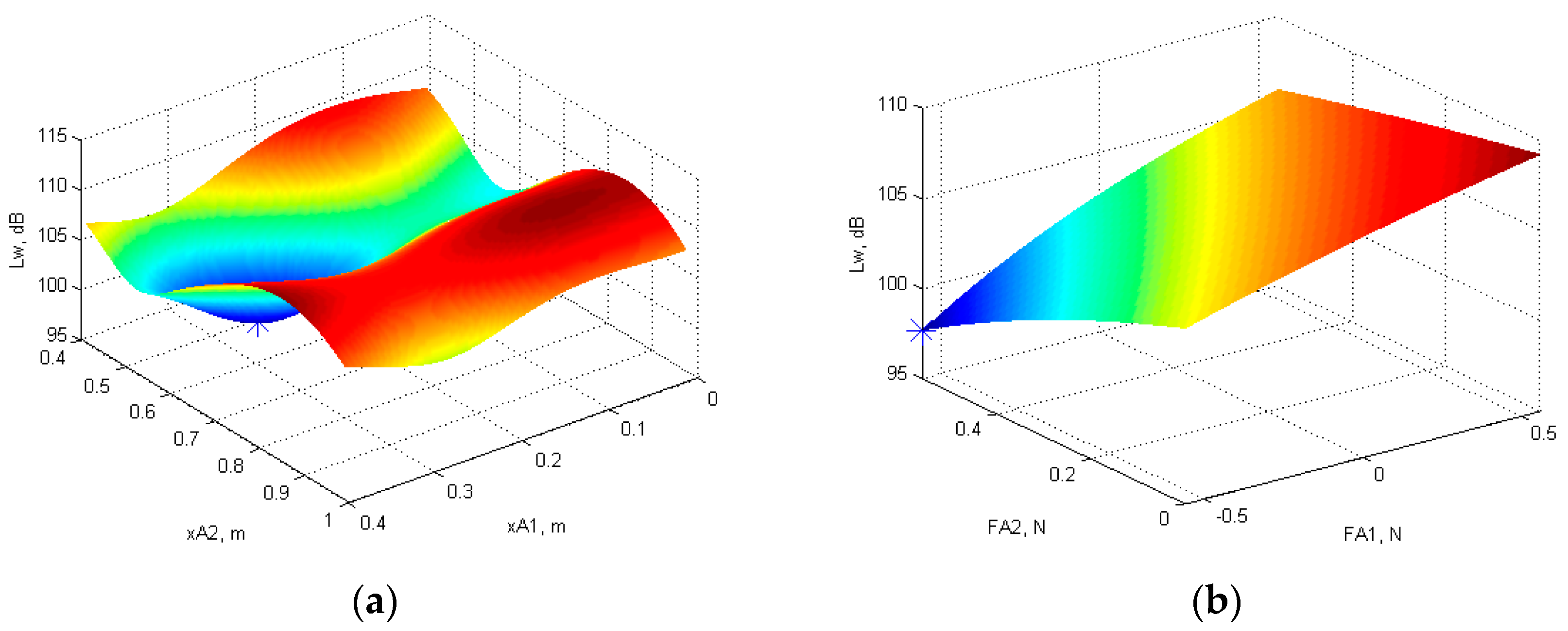
This paper presents a method for efficiently determining the parameters of the minimum total sound power level (Examples 3.2–3.4) based on the fact that the individual mode shapes have the most impact on the total sound power level. It was also proven that the minimum of the total power of the whole spectrum is close to the total power of the reference mode shapes. The optimization problem is solved using the sequential quadratic programming (SQP) method [
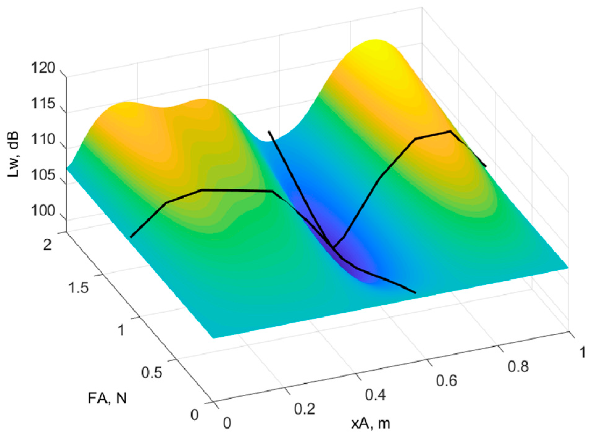
21]. The objective function, i.e., the total sound power level calculated using Equation (27) obtained with four reference mode shapes, is optimized in the presence of constraints on optimization variables. The optimization variable in Example 3.2 is the position of one actuator. The optimization variables in Example 3.3 are the position and amplitude related to one actuator, and in Example 3.3 are the position and amplitude related to two actuators. Details of the constraints on optimization variables are given as a part of the presented examples in the text that follows.

3. Examples

3.1. Comparison of Sound Power Calculations

In this example, the sound power level of a simply supported beam with the length of L = 1 m, the rectangular cross section of the height h = L/640, and the width b = L/64 was calculated. The harmonic load force with the amplitude FF = 1 N is applied at the position of xF = 0.85 L. The actuator with the amplitude FA = 0.6 N is applied in phase with the load at the position of xj = 0.4 m. A material with the density ρg = 7865.77 kg/m3 and the modulus of elasticity E = 2.1·1011 Pa is chosen. The damping in the material is considered to be small and is not considered. The ambient air has the density ρ = 1.2041 kg/m3 and the speed of sound in the air is c = 343.26 m/s.
The sound power level was calculated for the frequency range 0–70 Hz, which includes the first four natural frequencies of the beam, and the step size of the frequency range is 0.2 Hz. Figure 2 shows the diagram of the sound power level (Lw) for the given parameters. The mark * in Figure 2 refers to the results in the literature ([20] Figure 2), where the width ratio b = L/64 was also used.
The same diagram shows the control values of the sound power level of the vibration of the beam obtained with the reference mode shapes (values marked with *), i.e., calculated using the analytical expression (22). Considering the fact that there are small proportions of other mode shapes in the resonance response of the observed mode shape, a small difference in the mean square surface velocity between the shape of the overall response in resonance and the corresponding mode shape was noticed (Table 1).
Table 1 shows that the total response at resonance is approximately equal to the response of the reference mode shape, which led the authors to the conclusion that the mode shape radiation efficiency expression (22) can be used to calculate the parameters that yield the minimum total sound power level.

3.2. Position of the Actuator for Minimum Total Sound Power Level

In this example, an attempt was made to determine the optimal position of the actuator that minimizes the total sound power level of the vibrating beam. The selected step of the actuator position in the simulation for the new estimation of the sound power level is 0.01 m (for xA in the range of 0.5 to 0.6 m) and 0.05 m otherwise. The results are shown in Figure 3.
If the actuator position is at the left or at the right end of the beam, it has no influence on the response of the beam, so that the sound power level is equal to the sound power of the beam under the influence of the basic excitation FF. It follows that the maximal possible reduction in the total sound power level can be seen from the ratio of the minimum value and the side values of the total sound power level LWtot in Figure 3b.
Based on the comparison of the results of two different methods for calculating the sound power, an agreement was found between the minimum of the total sound power level calculated for the entire spectrum and the minimum of the total sound power level of the reference mode shapes for which the total sound power level was calculated according to the following expression:
L W t o t , r e f . m o d e s = 10 l o g j = 1 n t o t 10 L W j 10
where LWj is the sound power level calculated for a forced frequency near the jth natural frequency, and ntot is the total number of natural frequencies in the calculation (in this paper ntot = 4).
From the diagram in Figure 3b, it can be seen that the total sound power level of the whole spectrum is slightly higher than the total sound power level of the reference mode shapes (1.16%), but also that their minimums match closely, indicating that an analytical method can calculate the optimal parameters very efficiently and with a considerably shorter computational time (within a minute). For comparison, the computational time of the analyzed numerical simulation for only one actuator position lasts 3 h or more depending on the computer configuration. A short computational time allows for a fast optimization of the solution for several parameters simultaneously, which was carried out in the third and fourth example. The mentioned approach of multi-parameter optimization and the use of the solution of the total sound power level for reference mode shapes was not observed by the authors in the existing published works [12,13,14,19].
The accuracy of determining the parameters for the total sound power level minimum from the reference mode shapes decreases as the damping in the system increases, because the difference in the sound power level in the resonant and surrounding domain decreases. However, the calculation of the sound pressure, i.e., the Rayleigh integral, is defined for beams with low damping whose mode shapes are approximately in phase or antiphase, which allows the use of pressure expressions of the form (14) [3], so that the applied methods are suitable for flat structures with small damping.

3.3. Optimal Position and Force Amplitude of the Actuator for Minimum Total Sound Power Level

With the proposed method, it is possible to determine the optimized parameters that give the minimum total sound power level with much shorter computational time. The above presented procedure was applied for the simultaneous determination of the optimal position and force amplitude of the actuator, as presented in Figure 4. The matching of the analytical values, i.e., those represented with the two black curves obtained for xAmin = 0.5695 m, and for FAmin = 1.1264 N, with the values calculated for the total spectrum, is more clearly presented in Figure 5a,b.
Other authors optimize the value of one parameter, while the other parameters are fixed [19]. The mentioned approach is used because of the large computational time. With the new approach, it is possible to obtain the optimal values with analytical expressions and simultaneously optimize several parameters to reach the solution faster. Afterward, the obtained solution can be checked on a narrower frequency spectrum with less computational time. The effect of changing the position and force intensity of the actuators on the radiated sound power level and the best solution are shown in Figure 4.

3.4. Optimal Position and Force Amplitude of Two Actuators for Minimum Total Sound Power Level

In this example, the objective is to optimize the position and amplitude of the force of two actuators to obtain a minimum total sound level. There are four cases of constraints on the optimization and the corresponding results are presented in Table 2. The objective of the analysis is to determine the optimal position and force of the actuators for a minimum total sound power level.
Case 1: The lower and upper bounds of the actuator’s positions are defined as 0 and 1 m, respectively, the maximum force is limited to FAmin/2 = 0.5632 N (as in Example 3.3) and the actuators act in phase with the harmonic loading. The optimal position is 0.5695 m and the force amplitude FAmin/2 for both actuators. The result is consistent with Example 3.3. where one actuator was optimized.
Figure 6a shows the influence of the position of two actuators with constant force amplitudes (FAmin/2) on the total sound power level. It can be seen from the Figure 6a that the calculated positions result in a minimum of the total sound power level, which confirms the calculation. Figure 6b shows the influence of the force levels of two actuators on the optimal positions (in this case 0.5695 m). From the Figure 6b it can also be seen that the calculated forces give the minimum of the total sound power, which confirms the calculation.
If the upper bound of the actuator 1 amplitude force is FA1 < FAmin and the upper bound of the actuator 2 amplitude force is FA2 = FAminFA1, the results show that both the actuators should be in the same position 0.5695 m and their intensities should be equal to the given maximum values.
In Figure 7. the influence of the actuator at the position 0.5695 m in phase with the harmonic load force on the total sound power level can be seen. The sound power level of the 1st and 2nd mode shape is increased, but the sound power level of the 3rd and 4th mode shape is more significantly reduced, resulting in the decrease of the total sound power level. The increase in the sound power level can be explained by the fact that the actuator acts in phase with the beam velocity at the actuator position for the 1st and 2nd mode shape, which increases their amplitude, and the actuator acts in antiphase with the beam velocity at the actuator position for the 3rd and 4th mode shape which reduces their amplitudes. It should also be noted that the change in the amplitude of one mode shape does not automatically define the change in the total sound power level, since the sound pressure generated by one mode can affect or excite the vibration of another [8].
Case 2: The lower and upper bounds of the actuator’s positions are defined as 0 and 1 m, respectively, the maximum force is FAmin/2 = 0.5632 N (as in Example 3.3), and the actuators act in antiphase to the harmonic load. The optimization resulted in three solutions; in the first, both actuators act opposite to the harmonic load at the position of 0.85 m, and in the second and third solutions, the positions are symmetrical (Figure 8a) and correspond to positions 0.2812 and 0.8580 m when the force intensity is maximum, i.e., 0.5632 N.
If the actuator 1, of which the position is limited to the left half of the beam, can have the upper bound of the amplitude force FA1 and the upper bound of the amplitude force of the actuator 2 is FA2 = FAminFA1, with the condition FA2 > FA1, the optimization results in similar positions of the actuators and the sum of their intensities is equal to FAmin (Table 2. Case 2, left and right column). From the given results it follows that in this case it is more favorable to position the actuator with the higher force closer to the harmonic load.
Case 3: The lower and upper bounds of the actuator’s positions are defined as 0 and 1 m, respectively, the maximum force is FAmin/2 = 0.5632 N (as in Example 3.3), actuator 1 acts in phase, while actuator 2 acts in antiphase with harmonic load. The optimization results are listed in Table 2. (Case 3), where it can be seen that the actuator acting in phase is positioned near the center of the beam, while the actuator acting in antiphase is positioned near the harmonic load.
This is the case with the best result for the total sound power (Figure 9) level when using the upper bound of amplitude equal to FAmin/2 and ignoring the case where the actuators act in the opposite direction to the harmonic load (Case 2, first solution). From the comparison of the sound power spectra for Case 2 and Case 3, a reduction of the sound power level at the multiple modes can be seen (Figure 10).
Case 4: Actuator 1 position range is from 0 to 0.4 m, the upper bound of the amplitude force of the actuator 1 is FAmin/2 = 0.5632 N, and the actuator can act in phase or in antiphase to the harmonic load, while the actuator 2 position range is from 0.4 to 1 m, the maximum force is FAmin/2, and the actuator can act in phase with the harmonic load. The optimization results in actuator 1 with amplitude FAmin/2 in antiphase to the harmonic load at position 0.2834 m and actuator 2 with the same force amplitude but in phase with the harmonic load at position 0.569 m. Case 4 gives a slightly more favorable result (Figure 11) than Case 1, although the actuators are on average farther from the load. The reason for this is that both the actuators act in antiphase with the velocity of the 3rd and 4th mode shape at the actuator positions.
If the upper bound of the actuators force amplitude is less than FAmin/2, for example Fmax = 0.3 N (Table 3), their positions are approximately the same as in the previously analyzed case with FAmin/2, while the total sound power level increases. It is important to note that Case 3 gives the best result, which indicates that the key input parameter for defining the optimal positions of the actuators is the position of the harmonic load.

4. Conclusions

The sound power level of a stationary vibrating structural surface can be noticeably reduced by selecting the optimal position, force amplitude, and phase of the added actuators. This paper proposes a method for faster determination of the optimal parameters to achieve the minimum total sound power level.
To simulate the vibrations of a flat construction element, a beam of constant rectangular cross-section was chosen, simply supported at its ends. In this paper, the Euler–Bernoulli theory and the mode superposition method are used to define the motion of the beam. The beam is placed in an infinite baffle, and the calculation of the sound power using the sound pressures in the near and far fields is described.
The method is based on the similarity of the total sound power level of the reference mode shapes and the total sound power level of the whole spectrum. This paper showed that the optimized actuator positions for both approaches match closely. In addition, due to the significantly reduced computational time, the proposed method for determining optimal parameters allows the simultaneous search for the optimum for several parameters, which, to the authors’ knowledge, has not been executed before in published works.
In this work, the position and force amplitude of one and two actuators operating in phase or in antiphase with a given harmonic load on a simply supported beam were optimized in the frequency range of the first four natural frequencies. The following conclusions were drawn from the optimization results:
-
When one or two actuators are applied in phase with a harmonic load, the optimization results are equal, i.e., two actuators act at the same position as one actuator and the sum of the force amplitudes of two actuators is equal to the force amplitude of one actuator.
-
If one actuator acts in antiphase with the harmonic load, its optimal position is always at the position of the harmonic load.
-
If two given actuators and the load cannot act in antiphase, the optimal positions of the actuators enable the actuator force to be in antiphase with the velocity of the excited mode shape.
-
The most influential input parameter for the optimization of the actuator position is the position of the harmonic load.

Author Contributions

Conceptualization, A.S., G.Š.R., D.L. and S.B.; formal analysis, A.S. and G.Š.R.; investigation, A.S., G.Š.R., D.L. and S.B.; methodology, A.S., G.Š.R. and S.B.; validation, A.S., G.Š.R. and D.L.; writing—original draft, A.S. and G.Š.R.; writing—review and editing, A.S., G.Š.R., D.L. and S.B. All authors have read and agreed to the published version of the manuscript.

Funding

This research was funded by the Croatian Science Foundation (grant number: IP-2019-04-8615), University of Rijeka (grant number: uniri-tehnic-18-139) and University of Rijeka (grant number: uniri-tehnic-18-225). This support is gratefully acknowledged.

Data Availability Statement

Not applicable.

Conflicts of Interest

The authors declare no conflict of interest.

References

  1. Dimino, I.; Aliabadi, F. Active Control of Aircraft Cabin Noise; Imperial College Press: London, UK, 2015. [Google Scholar]
  2. Preumont, A. Vibration Control of Active Structures, 2nd ed.; Kluwer Academic Publishers: Dordrecht, The Netherlands, 2003. [Google Scholar]
  3. Fahy, F.; Gardonio, P. Sound and Structural Vibration: Radiation, Transmission and Response, 2nd ed.; Academic Press: London, UK, 2007. [Google Scholar]
  4. Nayan, A.; Kam, T.Y. Sound enhancement of orthotropic sound radiation plates using line loads and considering resonance characteristics. Acoustics 2021, 3, 642–664. [Google Scholar] [CrossRef]
  5. Wei, L.; Sheng, L. Mutual-radiation efficiency estimation of vibration modes by finite element method and boundary element method software. J. Low Freq. Noise Vib. Act. Control 2022, 41, 1131–1142. [Google Scholar] [CrossRef]
  6. Keltie, R.F.; Peng, H. The effects of modal coupling on the acoustic power radiation from panels. J. Vib. Acoust. Stress Reliab. Des. 1987, 109, 48–54. [Google Scholar] [CrossRef]
  7. Snyder, S.D.; Tanaka, N. Calculating total acoustic power output using modal radiation efficiencies. J. Acoust. Soc. Am. 1995, 97, 1702–1709. [Google Scholar] [CrossRef]
  8. Li, W.L.; Gibeling, H.J. Determination of the mutual radiation resistances of a rectangular plate and their impact of the radiated sound power. J. Sound Vib. 2000, 229, 1213–1233. [Google Scholar] [CrossRef]
  9. Ringwelski, S.; Luft, T.; Gabbert, U. Piezoelectric controlled noise attenuation of engineering systems. J. Theor. Appl. Mech. 2011, 49, 859–878. [Google Scholar]
  10. Lan, L.; Cheng, S.; Sun, X.; Li, W.; Yang, C.; Wang, F. A fast singular boundary method for the acoustic design sensitivity analysis of arbitrary two-and three-dimensional structures. Mathematics 2022, 10, 3817. [Google Scholar] [CrossRef]
  11. Cheng, S.; Wang, F.; Wu, G.; Zhang, C. A semi-analytical and boundary-type meshless method with adjoint variable formulation for acoustic design sensitivity analysis. Appl. Math. Lett. 2022, 131, 108068. [Google Scholar] [CrossRef]
  12. Makarenko, V. Modeling and control of sound radiation by simply supported and cantilever beam coupled with smart material. Vìsnik NAU 2007, 3, 142–150. [Google Scholar] [CrossRef]
  13. Anderson, D.A.; Heilemann, M.C.; Bocko, M.F. Optimized driver placement for array-driven flat-panel loudspeakers. Arch. Account. 2017, 42, 93–104. [Google Scholar] [CrossRef]
  14. Kournoutos, N.; Cheer, J. A system for controlling the directivity of sound radiated from a structure. J. Acoust. Soc. Am. 2019, 147, 231–241. [Google Scholar] [CrossRef] [PubMed]
  15. Wrona, S.; Pawelczyk, M.; Cheer, J. Acoustic radiation-based optimization of the placement of actuators for active control of noise transmitted through plates. Mech. Syst. Signal. Process. 2021, 147, 107009. [Google Scholar] [CrossRef]
  16. Rao, S.S. Vibration of Continuous Systems; John Wiley & Sons, Inc.: Hoboken, NJ, USA, 2007. [Google Scholar]
  17. Rončević, G.Š.; Rončević, B.; Skoblar, A.; Žigulić, R. Closed form solutions for frequency equation and mode shapes of elastically supported Euler-Bernoulli beams. J. Sound Vib. 2019, 457, 118–138. [Google Scholar] [CrossRef]
  18. Skoblar, A.; Žigulić, R.; Braut, S. Numerical ill-conditioning in evaluation of the dynamic response of structures with mode superposition method. Proc. Inst. Mech. Eng. C J. Mech. Eng. Sci. 2017, 231, 109–119. [Google Scholar] [CrossRef]
  19. Zaporozhets, A.; Tokarev, V.; Hufenbach, W.; Taeger, O.; Modler, N.; Dannemann, M.; Makarenko, V. Parametric investigation of acoustic radiation by a beam under load and actuator forces. Vìsnik NAU 2005, 26, 122–133. [Google Scholar] [CrossRef]
  20. Wallace, C.A. Radiation resistance of a baffled beam. J. Acoust. Soc. Am. 1972, 51 Pt 2, 936–945. [Google Scholar] [CrossRef]
  21. Schittkowski, K.; Yuan, Y.X. Sequential Quadratic Programming Methods. In Wiley Encyclopedia of Operations Research and Management Science; John Wiley & Sons, Inc.: Hoboken, NJ, USA, 2011. [Google Scholar] [CrossRef]
Figure 1. Beam parameters.
Acoustics 05 00027 g001
Figure 2. Sound power level spectrum (comparison with published results in [20] marked with *).
Acoustics 05 00027 g002
Figure 3. Diagram of (a) the sound power level and (b) the total sound power level for different actuator positions.
Acoustics 05 00027 g003
Figure 4. Total sound power level as a function of actuator position and force amplitude.
Acoustics 05 00027 g004
Figure 5. Total sound power level as a function of the actuator (a) position and (b) force amplitude.
Acoustics 05 00027 g005
Figure 6. The influence of (a) the position of two actuators with constant force amplitudes and (b) force amplitudes with constant actuator position, on the total sound power level for Case 1.
Acoustics 05 00027 g006
Figure 7. Sound power level spectra with one actuator (Case 1) and without the actuator (comparison with literature [20] marked with *).
Acoustics 05 00027 g007
Figure 8. The influence of (a) the position of two actuators with constant force amplitudes and (b) force amplitudes with constant actuator position on the total sound power level for Case 2.
Acoustics 05 00027 g008
Figure 9. The influence of (a) the position of two actuators with constant force amplitudes and (b) force amplitudes with constant actuator position on the total sound power level for Case 3.
Acoustics 05 00027 g009
Figure 10. Sound power level spectra for Case 2 and Case 3.
Acoustics 05 00027 g010
Figure 11. The influence of (a) the position of two actuators with constant force amplitudes and (b) force amplitudes with constant actuator position on the total sound power level for Case 4.
Acoustics 05 00027 g011
Table 1. Comparison of average mean square velocities.
v ω 2 1. Mode Shape2. Mode Shape3. Mode Shape4. Mode Shape
Total response29.54265.2018155.355994.9151
Ref. m. shape29.62085.1174155.253194.2995
Table 2. Optimal position and force amplitude of two actuators.
Case 1Case 2Case 3Case 4
F A 1 , N 0.5632−0.5632−0.32640.5109−0.5632
x A 1 , m 0.56950.28120.27840.57480.2834
F A 2 , N 0.5632−0.5632−0.8000−0.56320.5632
x A 2 , m 0.56950.85790.85920.83690.5690
L W t o t . m i n , d B 98.37993.198283.547191.155297.6596
Table 3. Optimal position and force amplitude of two actuators with upper bound Fmax = 0.3 N.
Case 1Case 2Case 3
F A 1 , N 0.3−0.30.3
x A 1 , m 0.5680.27870.5672
F A 2 , N 0.3−0.3−0.3
x A 2 , m 0.5680.8560.8542
L W t o t . m i n , d B 102.2909102.2606100.801
Disclaimer/Publisher’s Note: The statements, opinions and data contained in all publications are solely those of the individual author(s) and contributor(s) and not of MDPI and/or the editor(s). MDPI and/or the editor(s) disclaim responsibility for any injury to people or property resulting from any ideas, methods, instructions or products referred to in the content.

