Reviving the Low-Frequency Response of a Rupestrian Church by Means of FDTD Simulation

Abstract

Rupestrian churches are spaces obtained from excavation of soft rocks that are frequently found in many Mediterranean countries. In the present paper the church dedicated to Saints Andrew and Procopius, located close to the city of Monopoli in Apulia (Italy) is studied. On-site acoustical measures were made, obtaining a detailed description of the acoustics in the current state pointing out, thanks to a combination of analysis techniques, the presence of significant modal behavior in the low frequencies, causing reverberation time to be about 2 s, four times longer than in the other bands, as well as being strongly dependent on source and receiver position (with variations of about 1 s when source is moved outside the chancel). However, as the church is characterized by significant degradation of surfaces and large amounts of debris cover the floor, the original acoustic conditions can be expected to somewhat differ. Acoustical modelling can be very helpful in grasping the original conditions, but given the small dimensions of the space, conventional geometrical acoustic prediction methods cannot be applied to simulate the low-frequency behavior. Thus, the present paper proposes an application of finite-difference-time-domain (FDTD) computation to simulate the low-frequency behavior and analyze a possible reconstruction of the original state. Results showed that a very good agreement was obtained between predictions and measurements, both in terms of resonance frequencies and reverberation times that differed by less than 5%. Modal response strongly affected the acoustical conditions also in the hypothetical reconstruction of the original state, although the sound field proved to be more uniform than in the current state.

1. Introduction

Rupestrian churches belong to the largest and most widespread group of artificial cavities of anthropic origin, often labelled as rocky or troglodytic settlements, which can be found all over the world [1]. However, in the Mediterranean area, they can be found in nearly every country, with some of them showing a significantly higher number, as outlined by a census of rocky sites in the Mediterranean area [2], from which Italy, Spain, and Turkey appear as the richest in settlements. Apulia (and the neighboring area of Matera), Sicily and Tuscany in Italy, Andalusia in Spain, and Cappadocia in Turkey showed the highest number of rocky sites, most frequently located in areas where soft stone in combination with meteorological agents already created natural caves that were subsequently enlarged and shaped according to the needs of the occupants. With reference to religious buildings, the sites in Southern Italy originated from the spreading of Greek monks following the iconoclastic prosecution in the Eastern regions but also from local communities that often found a safe place far from the frequent aggressions arriving from the sea. In Spain, many sites were built by the Mozarabic population during the Moorish occupation of the South. In Cappadocia the churches can be found in settlements of cenobite monks that developed from 6th and 7th century after the introduction of the Christian cult [3], but it is not unusual to also find mosques in some places.

The shape of the rupestrian churches usually recalled that of ordinary architectures of the time, with the obvious limitations related to the characteristics of the site and the nature of the stone, but it is not unusual to find spaces that may well compete in dimension and complexity with ordinary churches.

Cave acoustics has attracted a considerable interest in the last years, starting with the seminal studies that tried to demonstrate that acoustic effects might have influenced the choice of the locations. Infrasonic resonances [4], echoes, and long resonances might have influenced mural paintings [5,6], as well as the use of sites as burial places [7]. Some studies [8,9] seem to agree with these hypotheses, also suggesting a deliberate use of such effects in the underground galleries of Chavin de Huantar in Peru [8]. More recently the topic has been further investigated by several large interdisciplinary groups [10,11,12,13], and other studies of cave acoustics have been carried out involving natural caves mostly [14,15,16] or burial places like catacombs [17].

When dealing with rupestrian churches and sacred spaces, the number of studies is significantly reduced [18,19], suggesting that many specific features of such spaces still need to be better disclosed and understood. One key issue in such spaces is represented by the bad conservation state, often related to locations far from urban areas, lack of controls, and exposure to any type of weather agents. Thus, current acoustic conditions may significantly differ from their original state, in most cases. It is important to underline that rupestrian churches were, first of all, “worship” spaces although their usage was not simply ascribed to individual celebrations by monks practicing ascetism, but they were used by whole communities of the settlements. Consequently, as rupestrian churches were used for ordinary masses, they had to deal with problems of speech intelligibility and propagation of the typical Byzantine hymns, inducing us to hypothesize correlations between acoustics and the shape and size of the spaces. For this reason, a reconstruction of the original acoustics of such spaces is of the utmost importance to understand which were the conditions in which the church was used and whether such correlations might exist.

Given the small dimensions of such spaces, modal behavior is likely to appear, resulting in non-uniform sound distribution at low frequencies, sound coloration (i.e., amplification or attenuation of certain frequencies), and strong variations of reverberation time as a function of narrow band frequencies. Modal behavior originates from standing waves that appear whenever the distance between the walls is a multiple of half wavelengths [20]. Axial, tangential, or oblique modes may appear depending on the number of surfaces that are involved in such standing wave paths.

Consequently, it is important to underline that simulating the acoustics of such spaces may be particularly challenging because of their small dimension which prevents a straightforward application of conventional methods based on geometrical acoustics which would be valid only well above the Schroeder frequency. Therefore, in such cases, it is essential to take advantage of different wave-based computational tools that may better describe the low-frequency behavior of the spaces. To this purpose, in this paper an application of the finite-difference-time-domain (FDTD) method is proposed, by implementing a simple scheme with frequency-independent boundary conditions limited to the lowest frequencies. Even though this method has been already applied to larger buildings and covering a much broader spectrum [21,22] using parallel computation on several graphical processing units, the present implementation aims at providing a useful low-frequency complement to conventional geometrical acoustic-based simulations, without requiring a high computational load.

The paper, taking advantage of the results already published in Ref. [19], will be organized as follows: Section 2 outlines the church that was surveyed, the acoustic measurement methods, the modelling techniques, and a few notes about FDTD; Section 3 presents the results of the on-site measurements, the results of the FDTD simulation in the current conditions, and the reconstruction of the original state; Section 4 provides a brief discussion of the results in comparison with other existing studies; finally, Section 5 summarizes the major conclusions.

2. Materials and Methods

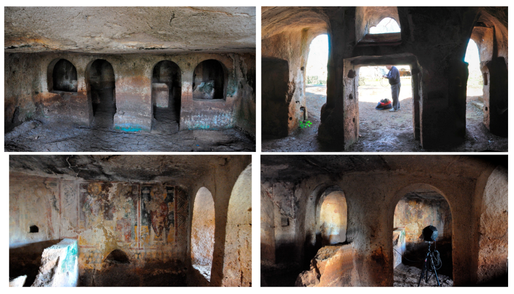
2.1. The Church Surveyed

The church of Saints Andrew and Procopius (Santi Andrea and Procopio) in Monopoli (Figure 1 and Figure 2) is located in the Contrada L’Assunta, along the Via Traiana and was likely built after the city of Monopoli was destroyed in 1042 to fight the Normans. The dedication of the church confirms the strong Byzantine influence as Andrew the Apostle was the founder of the church of Constantinople, and Procopius, martyr of Caesarea, was the protector of the Byzantine armies. The church was at the center of a rock village which also served as a post station along the Via Traiana (later Francigena) made up of a large number of caves with two or more rooms, oil mills, and mills [23].

The facade, just like in a masonry temple, has three arched entrances. The church is divided in two parts, the “naos” occupied by the congregation, having a simple rectangular shape (about 5.6 m by 5.2 m) and the chancel, divided by means of a “templum” (i.e., a stone iconostasis). The chancel was subdivided into four squares, two of them (the farthest from the entrance) define the “bema” where the altar was located. The ceiling is flat and its current height varies between 1.90 m and 2.40 m, but the original height is likely to be greater as a large amount of debris covers the floor. All the walls were originally covered by frescos but only a few fragments may be admired today.

Among the frescoes on the walls that are still visible, there are the apostles Peter and Paul, the saints Cosma, Damiano, Eligio (with the symbols of his patronage over the blacksmiths), Giorgio, Leonardo, a Virgin in throne and a scene of the Annunciation, datable between the 13th and 14th centuries. The painted scenes are all found in the bema and transept: Annunciation, Deesis, Trinity, Crucifixion, while the saints instead occupy the walls of the naos. The wall decoration is not contemporaneous with the excavation of the crypt but was constructed two centuries later. However, it reflects the continuity of worship from the Norman age, to which Saints Peter and Paul, Leonardo and Eligius belong, for example, up to the period of the Crusades (see, for example, the fresco of Saint George with the emblem of the cross on the saddle and on the shield). Unfortunately lost is the Byzantine iconography of the eleventh century relating to the eponymous saints of the sanctuary.

From the point of view of the liturgical functions, the church had the bema closed by a first iconostasis in stone opened by two doors in correspondence with the two apses. The transverse arm of the transept separates the presbytery from the naos, a common quadrangular room, not divided by pillars, with a second iconostasis, also with two doors. A summary of the main geometrical features is given in

Table 1. Summary of geometrical data and surface finishing.

Volume	113 m3
Plan surface	57 m2
Total area	210 m2
Average height	2.15 m
Surface openings	5 m2
Floor	Dry ground with large cracks
Ceiling/vault	Extremely rough and peeling tuffaceous stone
Wall	Strongly degraded tuffaceous stone, with evident signs of erosion and, in some points, covered by frescoed plasters also with evident signs of superficial deterioration

.

2.2. Acoustic Measurement Methods

Given the location of the church in an open field, all the measurements were carried out with portable instruments powered with battery packs. An omni-directional sound source (Lookline D301) was located in two positions, one in front of the altar (Position A) and one in the congregation area (Position B), so as to simulate in this way the priest and the congregation, respectively. The source was fed by an equalized sine sweep played back by a portable music player and generated using MATLAB (v. 2021b) according to Müller and Massarani [24] so that the spectrum of the radiated sound was substantially flat from 50 Hz to 16 kHz. The duration of the sweep was kept short (about 8 s) in order to limit any potentially adverse effects due to lack of doors, which, determining significant air circulation, might compromise the linear and time-invariant hypothesis. In addition, given the conservation state of the surface finishing, longer sine sweeps might have induced excess mechanical stress, so it was preferred to keep signals short. Given the limited dimensions of the space, the signal-to-noise (S/N) ratio was sufficiently high to ensure perfectly usable impulse responses, even if a short sweep was used. Room responses were collected using a portable B-format microphone (Soundfield ST-350) connected to a multi-channel recorder (Tascam DR-680) and a pair of binaural microphones (Soundman OKM II) worn by one of the authors and connected to a second recorder (Tascam DR-07). The measurement chain was previously tested in the lab to ensure that the “open loop” settings did not create any sync problem.

All the measurements were carried out complying with ISO 3382-1 [25] standard and taking into account the guidelines for measurements in worship spaces [26], and, despite the small dimensions of the church, eight receiver positions were used to provide a detailed description of the point-by-point variations. Microphones were placed at 1.6 m from the floor, assuming that the congregation was standing during the celebration. Source and receiver locations were chosen to provide a description of acoustical conditions that could be produced by actual sound sources and heard by listeners distributed in the space. Given the small dimension of the churches, only one person stayed in the room during the measurements.

Impulse responses (IR) were calculated by deconvolving the signal used to feed the sound source and, despite a significant background noise due to birds and other natural sounds (resulting, on average, in an A-weighted sound pressure level of 45 dB), provided a minimum S/N ratio of about 55 dB over the whole spectrum of interest. The measured IRs were then processed in order to calculate the most important acoustic parameters and to investigate room resonances. In particular, in addition to monaural parameters based on the omni (W) response of the B-format microphone, lateral energy fraction was calculated using W and Y Ambisonic components (assuming X axis was aimed at the source), while inter-aural cross correlation was based on binaural responses.

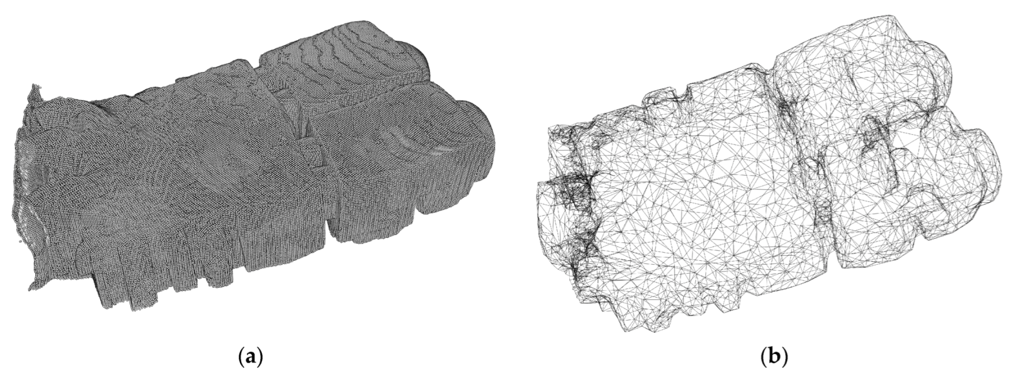
2.3. Geometrical Modelling of the Space

Given the complex and irregular shape of the space, the only reasonable way to obtain a reliable geometrical model was to use 3D laser scanning. A point cloud of more than 150k elements was originally obtained using a Riegl VZ 400 scanner (with an original resolution of 5 cm), but for the purpose of the simulation, such level of detail was unnecessary and thus, after cleaning artifacts and imperfections using a specifically designed tool developed in MATLAB, the point cloud was further simplified using the open source software Meshlab through subsequent applications of the “Quadric Edge Collapse Decimation” algorithm (Figure 3).

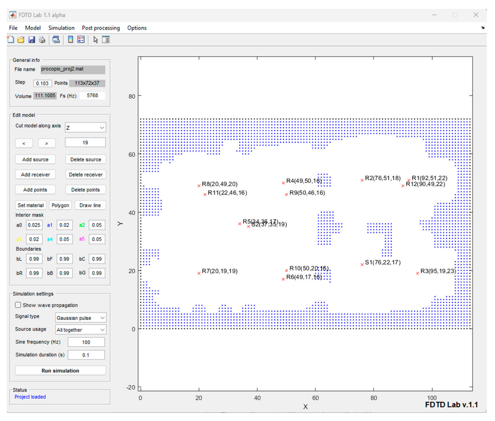
2.4. FDTD Simulation

FDTD acoustic modelling has been applied to solve acoustic problems for a long time [27] but given the computational load it has been mostly applied to low frequencies [28], while the availability of parallel computation distributed by several GPUs fostered a gradual extension to a much wider frequency range [21,22,28,29,30]. FDTD starts from the assumption that a generic derivation operator can be replaced by one of its finite difference forms:

$$\frac{df}{dx}\left(x_0\right)\approx \frac{f\left(x_0+\Delta x\right)-f\left(x_0\right)}{\Delta x}$$

(1)

and hence the second-order derivative becomes:

$$\frac{d^{2}f}{d{x}^2}\left(x_0\right)\approx \frac{f\left(x_0+\Delta x\right)-2f\left(x_0\right)+f\left(x_0-\Delta x\right)}{\Delta x^2}$$

(2)

In acoustics, any propagation phenomenon is described by the wave equation expressed by:

$${\nabla }^{2}p=\frac{1}{c^2}\frac{{\partial }^{2}p}{\partial t^2}$$

(3)

The equation is only expressed as a function of sound pressure p, but its finite-difference form would require three different time steps to be numerically solved, so in a 2D case in which T is the time step and X is the grid spacing, pressure at step n + 1 and node (x,y) will be given by:

$$p_{x,y}^{n+1}={\lambda }^2\left(p_{x+1,y}^n+p_{x-1,y}^n+p_{x,y+1}^n+p_{x,y-1}^n\right)+2\left(1-2{\lambda }^2\right)p_{x,y}^n-p_{x,y}^{n-1}$$

(4)

where λ = c T/X, c being the speed of sound in air. However, considering that the wave equation is derived by two other fundamental equations, involving only first-order derivatives, but also including particle velocity, it is possible to find a perfectly equivalent [29,30] alternative formulation. This formulation is known as staggered Yee’s grid, in which the grid of the pressure values is complemented by the grid of the particle velocity values (u). Thus, it is possible to first update particle velocity components (remembering that particle velocity is a vector quantity and, in 2D, it will have ux and uy components) and when this matrix is available, we can update the pressure at the next time step. Pressure at step n + 1 and node (x,y) will consequently be given by:

$$p_{x,y}^{n+1}=p_{x,y}^n-\frac{\rho c^2\mathrm{T}}{\mathrm{X}}\left(u{x}_{x+0.5,y}^{n+0.5}-u{x}_{x-0.5,y}^{n+0.5}\right)-\frac{\rho c^2\mathrm{T}}{\mathrm{X}}\left(u{y}_{x,y+0.5}^{n+0.5}-u{y}_{x,y-0.5}^{n+0.5}\right)$$

(5)

The above equations apply when non-boundary conditions are found, while at grid points close to walls, assuming a wall impedance Z, it is possible to find an update formula that, in case Z may be considered a real number independent of frequency, yields (in the 2D case) [31]:

$$u{x}_{x,y}^n=\frac{R_x-Z}{R_x+Z}u{x}_{x,y}^{n-1}+\frac{2}{R_x+Z}{p}_{x-0.5,y}^{n-0.5}$$

(6)

where R_x = ρ T/X, ρ being air density, and Z= ρ · c {[1 + (1 − α)^0.5]/[1 − (1 − α)^0.5]}, with α being the absorption coefficient of the given surface. A number of alternative approaches have been proposed to account for frequency dependence [27,32], but in the present case, being the analysis limited to the low-frequency case, the proposed assumption was not considered a major limitation.

In order to obtain a reliable calculation using FDTD, it is essential to properly set grid spacing X and time step T. In fact, they are both related to the maximum frequency that can be analyzed, as a minimum of five points per wavelength is usually required to prevent errors. Therefore, this means that given the minimum wavelength of interest (λ), the grid spacing should be at least λ/5 or, better, λ/10. Thus, for a grid spacing of 0.1 m, the FDTD results will be accurate up to a maximum frequency of 340 Hz. The time step is not independent of the grid spacing if the stability condition given by:

$$T\le \frac{X}{c\sqrt{D}} ,$$

(7)

(where D is the number of dimensions of the problem) is satisfied. Thus, once the grid spacing and the problem dimension are defined, time step results consequently (in the present case corresponding to a sampling frequency of 5768 Hz). Proper limitation of the highest frequency of analysis is also useful to minimize dispersion errors that result in phase velocity being different from the actual value of the medium. In the present case, limiting to frequencies below 340 Hz ensures that dispersion errors will be below 2% [29].

The previously described FDTD framework was implemented in MATLAB (Figure 4), where the geometrical model was first voxelized using a 10 cm grid spacing, and then surface properties could be assigned together with source and receiver locations. Sound sources were modeled as simple point sources and emitted signals could vary between sine waves (for modal analysis) and short pulses.

As per usual, surface properties were adjusted in order to have a suitable match between measured and predicted values of the reverberation time in the present condition at frequencies of 63 Hz and 125 Hz.

It is important to point out that for a space of such dimensions (113 m³), it is essential to model sound propagation by means of wave-based models because geometrical acoustics can only be effective well above Schroeder’s frequency that, being equal to $2000\sqrt{T/V}$, in this case was around 250 Hz. For this reason, modal response was also carefully compared to ensure that the model could realistically reproduce low-frequency propagation.

2.5. Material Characterization

In order to characterize sound absorption of the tuffaceous surface of the church, samples taken from quarries of geologically similar limestone were analyzed. Measurements of normal incidence sound absorption coefficient were carried out according to ISO 10534-2:1998 [33], using the transfer function method. As the objective of the study was to understand the low-frequency behavior of the materials, only the tube with an internal diameter of 10 cm was used, resulting in a maximum measurable frequency of 2 kHz and a low-frequency limit of 50 Hz. The emitting end consisted of an 11 cm loudspeaker sealed into a wooden case and suitably isolated from the tube structure by an elastic and protective layer. All the processing was performed by a MATLAB graphic user interface generating a linear sweep to feed the loudspeaker.

As shown in

Table 2. Summary of measured normal incidence absorption coefficients of different limestone samples 5 cm thick.

Material	63 Hz	80 Hz	100 Hz	125 Hz	160 Hz
Soft limestone (Carparo)	0.010	0.020	0.030	0.050	0.080
Hard limestone	0.010	0.020	0.020	0.024	0.037

, the major difference between different types of tuffaceous stones appears above 80 Hz, where higher porosity may contribute to nearly double absorption compared to harder samples. At very low frequencies, no significant differences were observed in the measured values.

3. Results

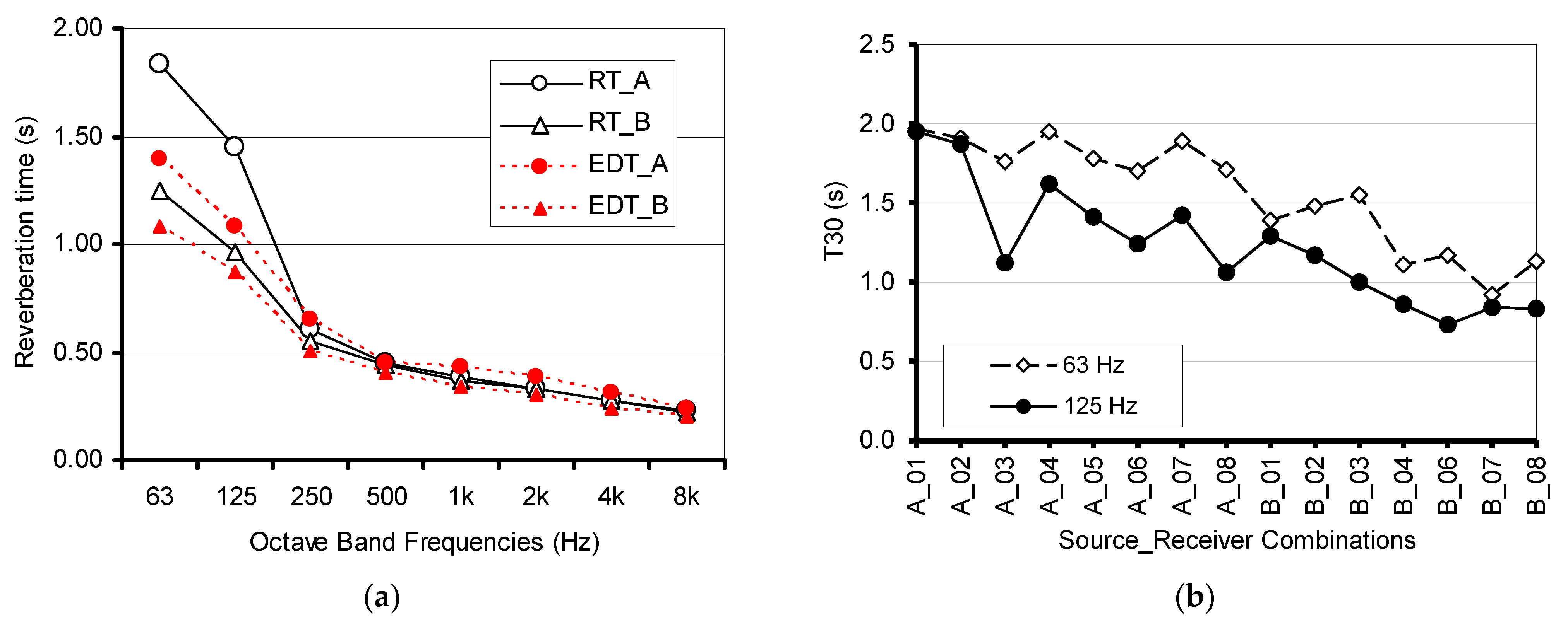
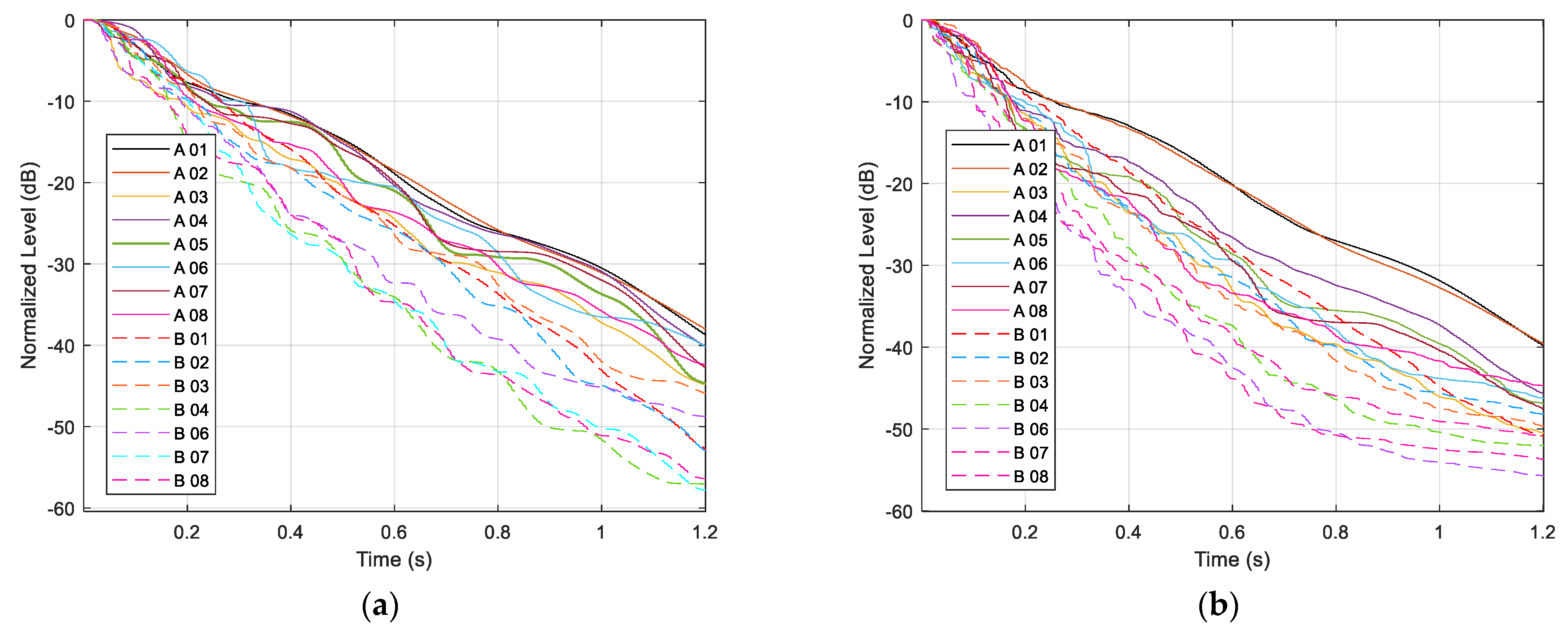
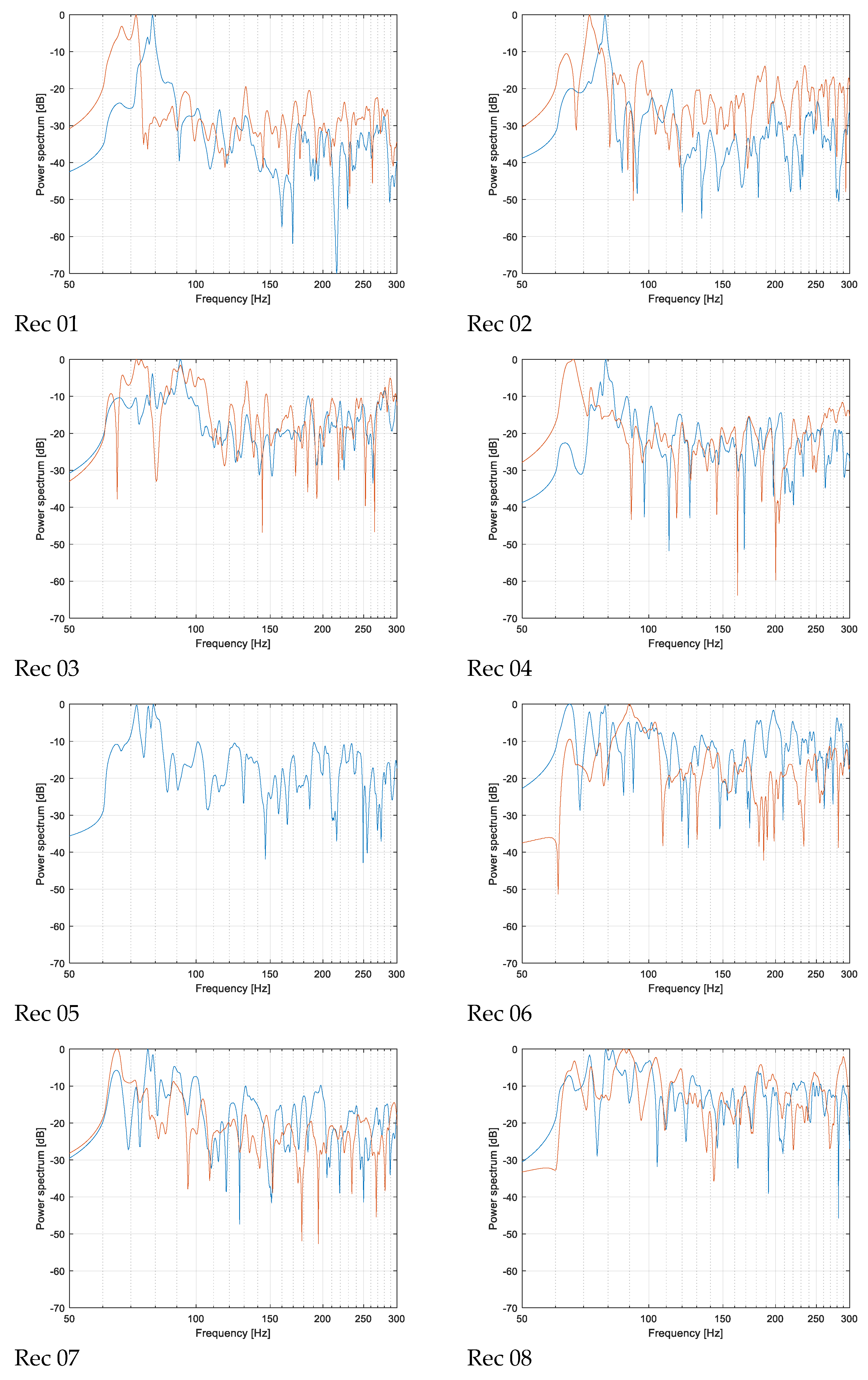
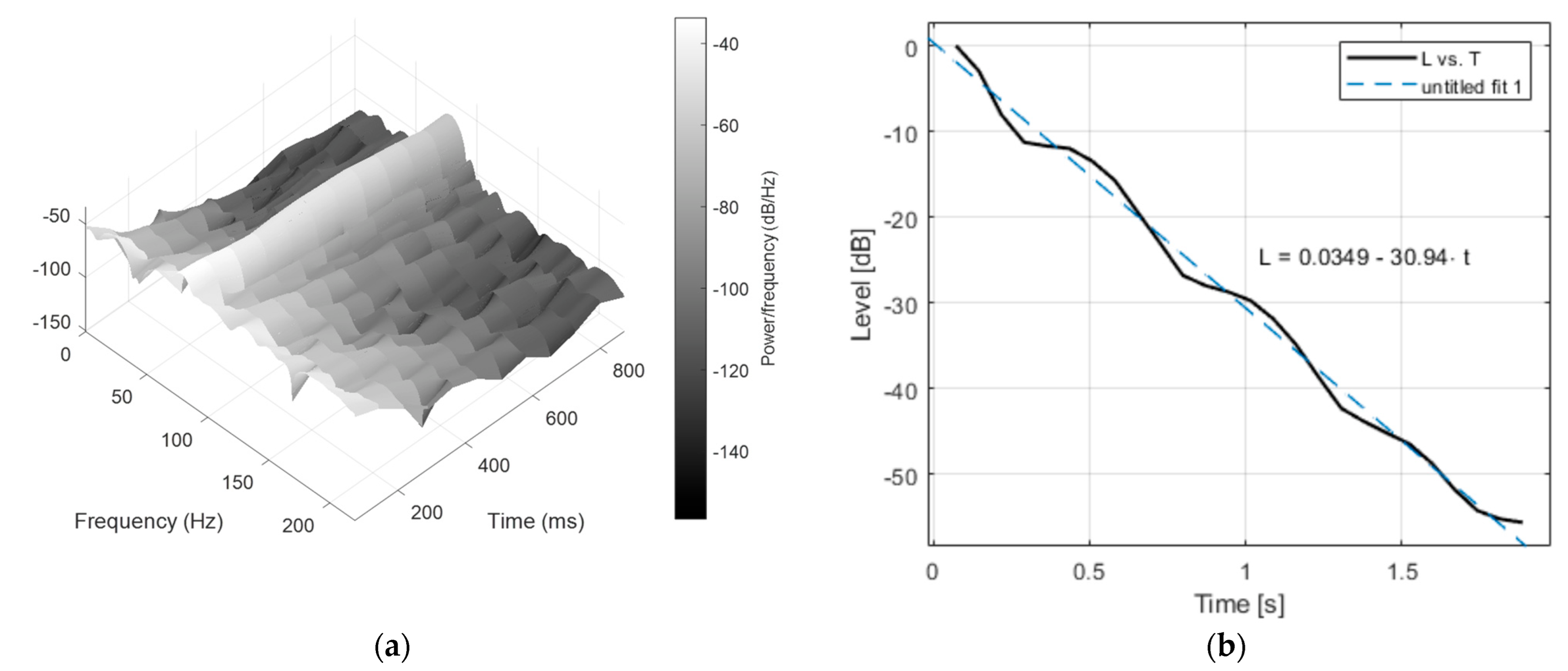
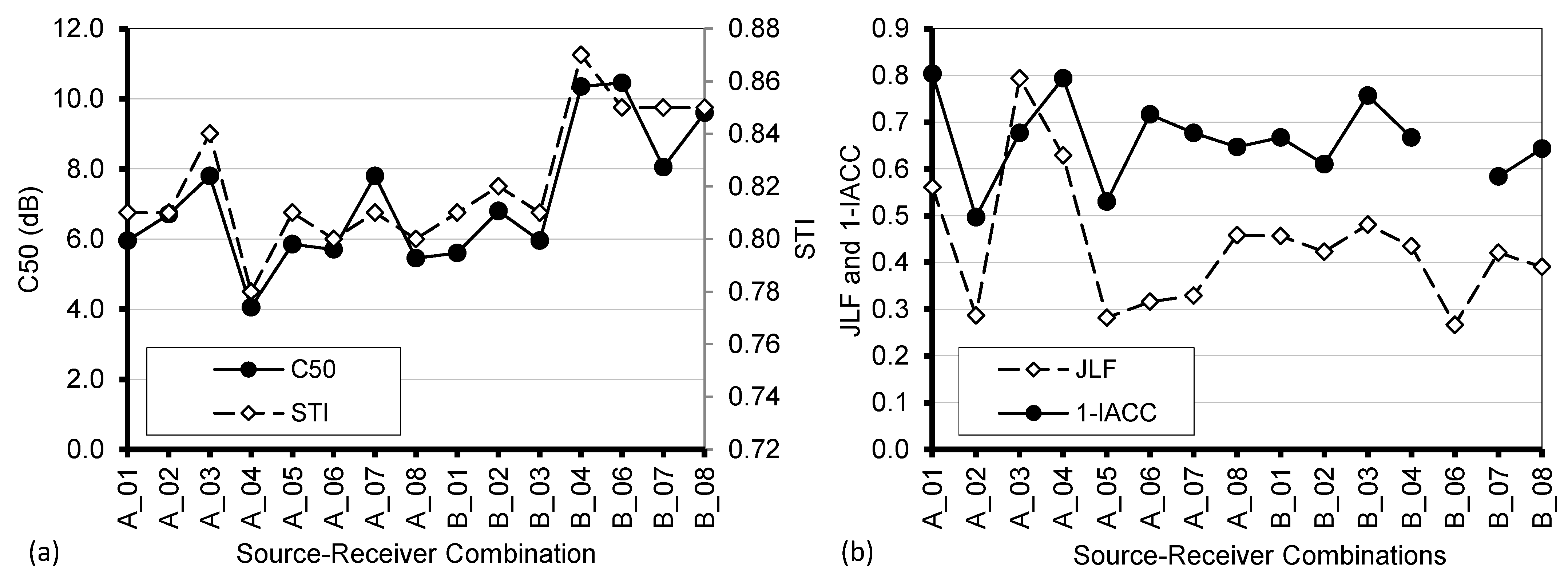
3.1. On-Site Acoustic Measurements

The analysis of the reverberation times shows very interesting differences between the medium-high frequencies, where the values settle below 0.5 s, with negligible point-by-point variations, and the low frequencies, where the values are considerably longer and show some variability depending on the location of both source and receivers (Figure 5). In particular, when the source was close to the altar (Source A), T30 at 63 Hz and at 125 Hz assumed the longest values (particularly at receivers 1, 2, 4, and 7), smoothly decreasing when moving closer to the entrance. When the source was in position B, T30 dropped by about 0.5 s in the same position. This fact, combined with EDT values shorter than T30 whatever the source position, suggested that no evident reverberant coupling effects between the sub-volumes may explain the observed variations. Conversely, the analysis of the time decays at 63 Hz and 125 Hz shows (Figure 6) that decays are characterized by a staircased or “pulsating” trend, clearly evident at 63 Hz, but also appearing at 125 Hz, in particular for combinations A_01 and A_02. Such behavior is typically associated with repeated reflections (flutter echoes) or modal effects which could be better investigated by analyzing the narrow band spectra of the responses.

Before delving into the analysis of the spectra, it is worth noticing that the short reverberation time at medium-high frequencies was likely due to the presence of openings (about 4 m²) and to the particular state of deterioration of the stone which appeared very pronounced, with frescoes occupying only a small part of the surfaces and the underlying layer characterized by greater porosity and tenderness. As shown in Table 2, a soft limestone is capable of absorbing a significantly higher amount of acoustic energy, which may easily explain the observed values. In addition, the floor was completely covered by waste soil overflowed during floods, characterized, at the time of measurement, by numerous cracks and having a thickness which could be estimated to vary between 10 cm and 50 cm in some points.

In order to better understand the observed low-frequency behavior, narrow band spectra were determined for all the source–receiver combinations (Figure 7). As expected, when source was in position A, receivers 1, 2, and 4 clearly showed a marked peak at 79 Hz, surrounded by many others appearing at 65 Hz, 73 Hz, and 87 Hz. In the other receivers, the same modes appeared but their energy content was significantly reduced. In fact, if the mid-frequency spectrum density is taken as a reference, the level variation around 79 Hz is about 30 dB between receivers 1 and 2 and the others.

When the source was moved into the “naos”, the acoustic energy redistributed among modes. In fact, the new absolute peak appeared around 65 Hz and 73 Hz at receivers 1, 2, and 4, while in the others the mode energy was more evenly distributed but remained at least 10 dB higher than in the frequencies above 100 Hz.

This can clearly explain what was observed in terms of reverberation time because the peak appearing around 80 Hz due to its position and magnitude influenced both the octave bands of 63 Hz and 125 Hz, causing the slower decay as observed in Figure 6 to appear in receiver 1 and 2 also in the higher octave band. In the other receivers, as the energy in the modes decreases, the reverberation time becomes gradually shorter, remaining longer in the 63 Hz band due to persistence in time of modal behavior (Figure 8a). To this purpose, modal reverberation time [34,35] was calculated for combination A-01 at the frequency of 78.2 Hz, showing (Figure 8b) that the observed value basically coincided with the octave band value.

The mathematics of the axial resonance modes [20] state that resonances appear at frequency f_n = (c ⋅ n)/(2L), where c is the speed of sound, L is the room dimension in the direction that is considered, and n is an integer index that defines the mode order. Thus, it can be easily found that 79 Hz corresponds to the first (n = 1) axial mode along the vertical direction assuming a height of 2.15 m (which is in good agreement with the average height of the space, although being far from a simple rectangular box), while 65 Hz corresponds well to the second (n = 2) axial mode along the two side walls (spaced by about 5.4 m), the only two large and continuous surfaces besides the floor and the ceiling.

Once the basic acoustical features have been explained by properly combining reverberation time and modal analysis, it is now possible to have a look at the other acoustical parameters (Figure 9). Given the short reverberation, very high speech intelligibility is obtained (STI = 0.82 on average) and strong frequency imbalance represented by a bass ratio (BR) equal to 2.1, although in the original conditions, with walls covered by frescos, it is likely that a more balanced condition was observed.

The perception of sound spatiality and, more generally, the binaural impression were particularly interesting. JLF and 1-IACC applied to the initial part of the impulse response showed rather high values (1-IACC = 0.67 on average) which were reduced only (as expected) in correspondence with the points placed in direct proximity to the source (receivers 2 and 5). The large amount of surface irregularities distributed almost everywhere, together with the presence of obstacles (such as the iconostasis) all contribute to this effect, making the sound perception very “spacious” despite the small size. JLF showed extremely high values deriving from the strong contribution of lateral reflections combined with the frequent shielding of reflections coming from frontal directions.

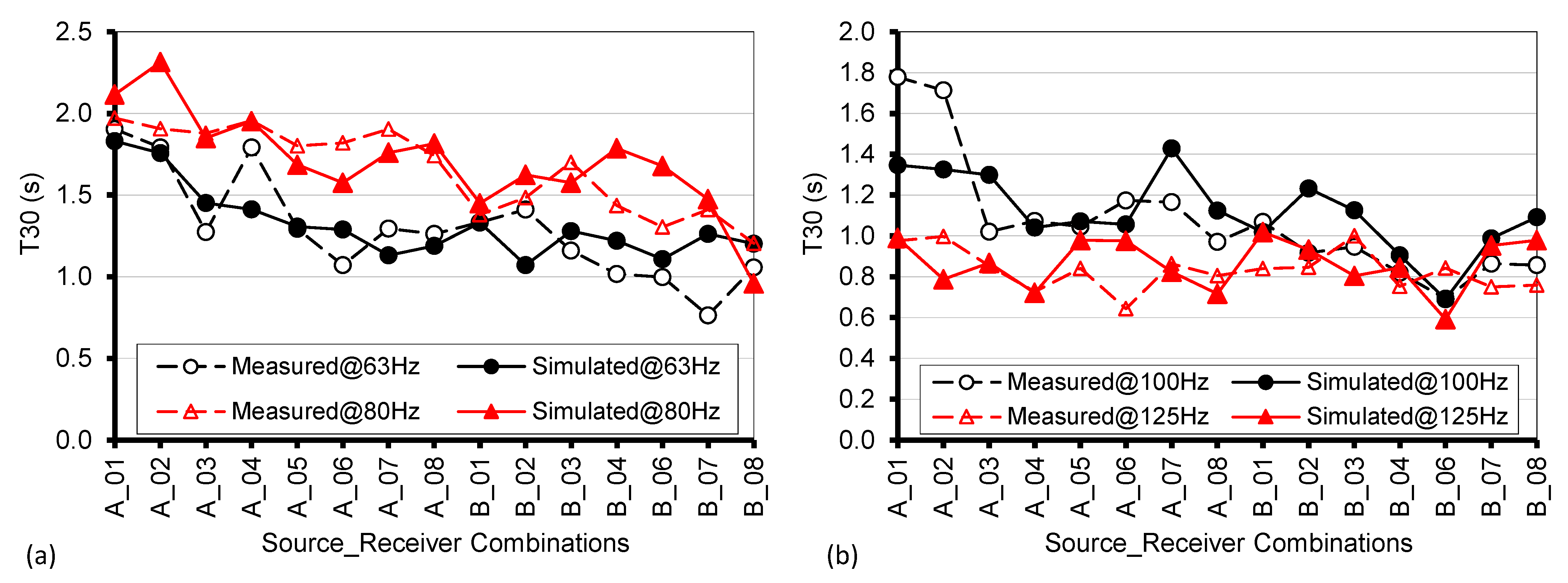
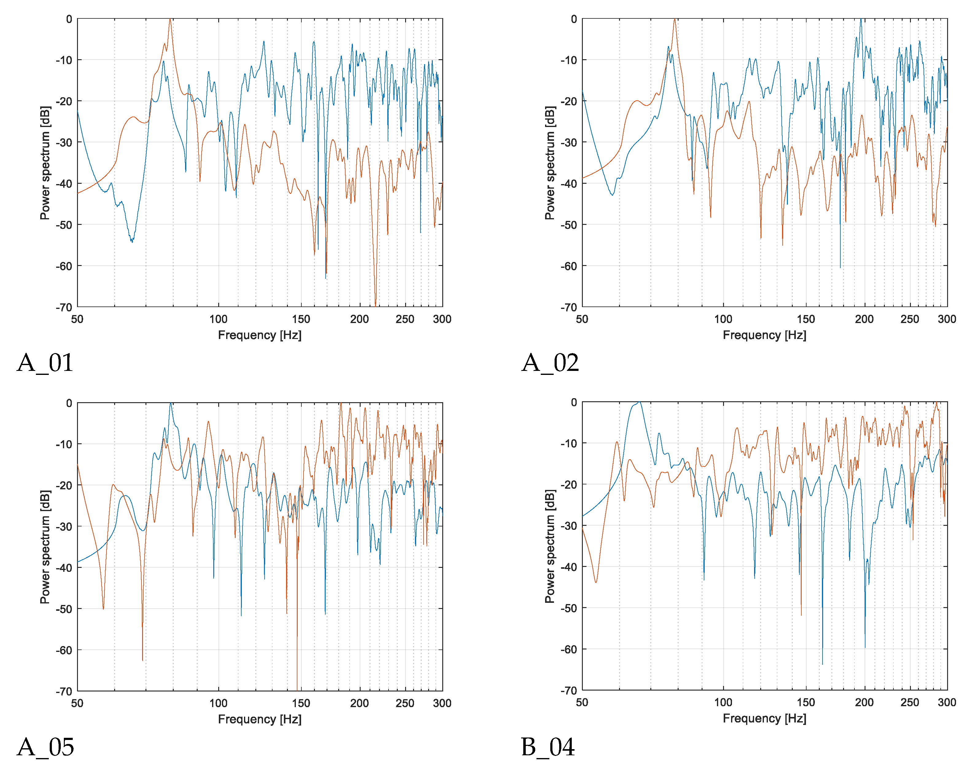
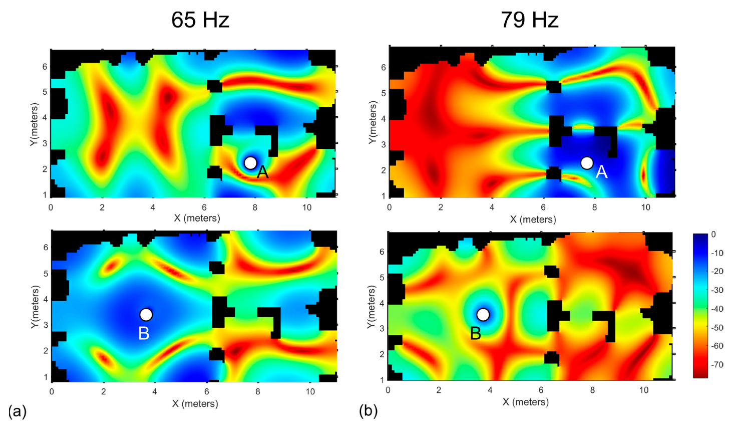
3.2. FDTD Acoustical Simulation of Current State

FDTD simulations were carried out according to the procedures described in Section 2.4. As the finishing was relatively the same over all the surfaces, with the notable exception of the floor covered by hardened soil, and given the values measured for similar materials (Table 2), an initial value of 0.015 was used for the absorption coefficient (obtained by averaging among the 63 Hz and the 125 Hz values). As this value returned slightly longer T30 values than expected, while in acoustic modelling [22] a maximum difference of 5% (corresponding to one just noticeable difference [25]), is considered to be acceptable, step-by-step increases were applied until a value of 0.025 was reached. Under these conditions, the spatial average of T30 in one-third octave bands from 63 Hz to 80 Hz differed by only 2% from measurements, while at 100 Hz the error was 4%. At higher frequencies, the error was bigger, suggesting that a further increase in absorption coefficient was needed. By adopting an α value of 0.04, the mean error was finally reduced to 4% also in the 125 Hz band. Figure 10 shows the comparison between measured and predicted reverberation time in one-third octave bands at individual positions. It can be observed that in the lowest bands clear modal behavior appears at given receiver positions, resulting from the strong non-uniform distribution of the values. In addition, as discussed in the previous section, the strength of the first axial mode along the vertical direction clearly appears also in the simulated results, where T30 in the 80 Hz band is markedly higher than the corresponding values at 63 Hz despite the same absorption coefficient. At 100 Hz and 125 Hz the modal behavior is significantly attenuated in the simulations (although the measured values at combinations A-01 and A-02 still show some effects).

Given the role played by modal response of the room, it was important to check the agreement between measured and predicted spectra. Considering that Figure 7 had already shown the combinations where a strong modal response was measured, the comparison was restricted to a subset of all the source–receiver combinations. Figure 11 shows that for combinations A-01 and A-02, the strong response around 79 Hz clearly appears, although the magnitude is attenuated compared to measurements assuming higher frequencies as a reference (which also explains why the 100 Hz T30 is shorter in the simulated response). Small shifts in the peak frequencies can be observed, but they rarely exceed 2 Hz. Combination A-05 is modelled pretty well, with the peak around 65 Hz well visible and a slightly less defined cluster around 79 Hz but a well comparable distribution of levels. Finally, combination B-04 is considered, as in the measured spectrum a clear peak appeared at 65 Hz. The simulated spectrum presents several peaks that are mostly aligned with measurements, but the stronger peak at 65 Hz seems more attenuated (by about 15 dB), and another peak below 60 Hz appears. However, considering that measured spectra were band-limited by the inherent frequency response of the sound source and by the signal used to feed the loudspeaker, this was considered a minor problem.

A further element to be considered that might explain some of the small differences observed in the T30 values and in the responses is the strong point-by-point variations that appear in consequence of the modal behavior. Taking into account the FDTD model, the sound pressure level resulting from pure tones at 65 Hz and 79 Hz was calculated for the two source positions. As shown in Figure 12, dramatic sound pressure level variations take place by simply moving the receivers a few centimeters apart. Hence, it is not unlikely that small misplacement of the receivers (both during the measurements and in the simulation setup) might explain some of the observed differences.

However, Figure 12 is quite instructive because it shows which are the positions in the church where stronger resonances appear and, consequently, where longer reverberation might be experienced. Predictably, receivers close to the side walls in the “naos” could experience strong resonances whatever the source position was, particularly at 65 Hz (which was the second axial mode along the transverse direction), but also at the other frequencies.

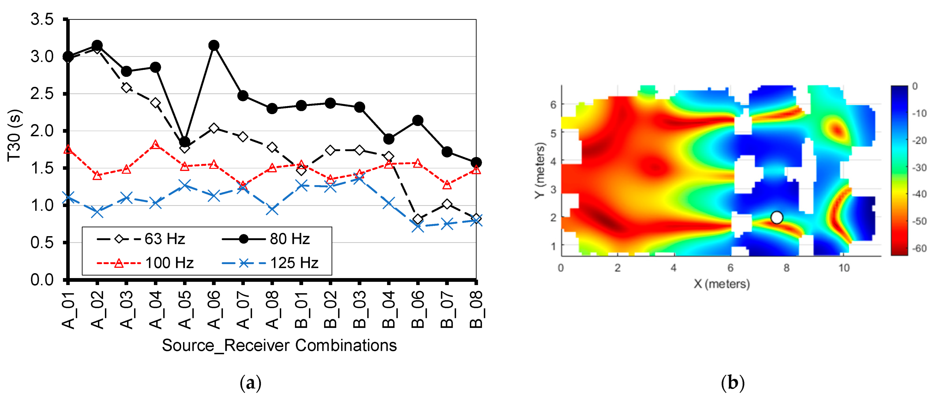
3.3. FDTD Acoustical Reconstruction of Original State

Once the model was calibrated, it could be used to apply a few changes that could realistically correspond to the original state, allowing us to appreciate the implications for the acoustics. In the specific case, three simple changes were applied. First, the floor area was rectified assuming that the layers of debris that currently occupy the entrance and the chancel area, where the ceiling is unusually low (see dashed line in Figure 1b), could be removed. Surfaces were considered to be covered by plasters and frescos (like the limited portions still existing clearly suggest, and like it is found in many other rupestrian churches in the region), resulting in a reduced absorption coefficient of 0.015 at 63 Hz and 80 Hz, and 0.025 at 100 Hz. Finally, in order to simulate acoustics under occupied conditions, a seated audience was located along the two side walls of the “naos”, according to the common practice of the time, as demonstrated by the usual presence of “subsellia” (carved benches) in other churches. This position was chosen in order to locate the absorption in the position where modal behavior might have more strongly affected the acoustic response in terms of damping. Absorption coefficients for this area were set to 0.2 [36] assuming the audience to be tightly distributed among the limited seats. All the openings were left in their actual state as no evidence of pre-existing doors or windows was found.

As shown in Figure 13, most of the main features observed in the “current” state also appear in the “reconstructed”, but now reverberation is longer and the modal response at 79 Hz when the source is in A is stronger and extends well beyond the “templum”. When the source is in B, the most evident variation is a drop appearing at receivers close to the entrance, possibly as a consequence of the change in room height (that is the part where the debris were thicker and after removal the ceiling height becomes about 2.7 m) and increase in the absorbing elements in the volume due to audience and increased opening surfaces (again as a consequence of debris removal).

Such results seem to suggest that the resulting acoustic effects might have been exploited during liturgical celebrations and singing, in particular, considering that the specific features of many Byzantine hymns include many bass notes sustained for a long time, which could well excite the resonances of the space.

4. Discussion

After presenting the results of the measurements and of the simulations, a brief discussion to put the results in the context of the existing literature can be developed. Among the spaces that have been surveyed by other authors, the highest similarity can be found with the rock-cut structures in Cappadocia [18]. Although the only space having a comparable volume was the Avanos dining room (114 m³), and the observed reverberation times spanned over a much broader range (up to 5 s for the Hallaç Church and main hall and for Açıksaray Hall), in all of the cases a significant low-frequency imbalance was observed, with reverberation time being up to 3 times longer than at mid-frequencies. This was likely caused by the characteristics of the stone that due to its porosity caused increased absorption as frequency grew. However, no specific low-frequency measures were made, and the frequency range of analysis was limited to 125 Hz.

Similarly, among the catacombs in Southern Italy [17], it was difficult to find spaces that are entirely comparable, but the two cubicles in the “San Callisto” catacombs have several similarities in terms of room dimensions and volumes. Materials are also similar, the walls being made of tufa stone, resulting in short reverberation times usually well below 1 s. In this case, the frequency range of the measurements extends into the 63 Hz band, showing only a moderate increase in reverberation time compared to mid-frequencies, with the notable exception of the so called “double cubicle”, where reverberation is longer (up to 1.5 s at 63 Hz) and characterized by point-by-point variations. Regardless, even in this study, although the “resonant” behavior in the low frequencies is supposed, no additional investigations were made.

Low-frequency resonances and modal behavior were investigated in many stone chambers and cairns in the British Isles [7]. In this case, experimental measurements were carried out using sine sweeps to find resonant frequencies and the distribution of nodes and antinodes in the space. A theoretical justification was consequently found based on the dimensions of the space, showing that in most of the cases, resonance frequencies varied between 95 Hz and 120 Hz, slightly above the resonances observed in the present work, likely as a consequence of the smaller dimension.

Finally, one interesting example where the modal behavior of a space was investigated also by means of wave-based acoustic simulation is the Ħal Saflieni Hypogeum [11]. In this Neolithic structure, the authors investigated the possibility that the resonance frequencies observed in different chambers have been “tuned” in some way. Based on the on-site measurements, a numerical model was developed to test whether different dimensions of the chambers might have altered this tuning. However, as in the present study, this reconstruction reflects the “current” conditions which might have been different from the original conditions which, as the authors clearly state, may be difficult to imagine.

5. Conclusions

In this paper, the case of the rupestrian church of Saints Andrew and Procopius in Monopoli (Apulia, Italy) was considered. The church has a small volume and is in a very bad conservation state, but it was acoustically analyzed in its current state by means of measurements carried out according to ISO 3382-1 standard. A combination of different analysis methods, including not only simple room acoustical parameters, as in most previous studies, but also spectrograms, modal reverberation time, and detailed maps based on FDTD modelling, were used to interpret the results. Measurements pointed out a singular behavior characterized by short reverberation times (around 0.5 s) at frequencies above 250 Hz, and much longer values in the lowest bands reaching up to 2 s, also in combination with strong resonances due to the modal response of the room. The analysis of the narrow band spectra and of modal reverberation time confirmed such dependance and resonant frequencies, especially those appearing at 65 Hz and 79 Hz, which were explained as a function of the room dimensions (although with some approximations due to the strongly irregular shape). In order to acoustically simulate the space and analyze the distribution of sound both in the current and in any possible reconstructions of the original state, given the small dimensions that make it impossible to use geometrical acoustic models in the low-frequency range, the numerical FDTD method was applied by using a proprietary code developed in MATLAB. Thanks to a laser scanner survey, the geometry was simplified and voxelized so that FDTD could be applied. Results showed a very good agreement both in terms of predicted reverberation time and modal response, implying that FDTD method, despite its simplified implementation, is the most reliable approach to simulate such small spaces and obtain time-dependent responses. Consequently, a simulation of a possible reconstructed condition, characterized by plastered surfaces, debris removed from the floor, and some occupants in the space, was carried out. Results showed that the strong modal response still appeared, suggesting that liturgical singing might have taken advantage of such specific acoustic features.

References

1. UNESCO World Heritage Centre. Available online: http://whc.unesco.org/ (accessed on 28 March 2023).
2. Bixio, R.; De Pascale, A.; Mainetti, M. Census of Rocky Sites in the Mediterranean Area. In The Rupestrian Settlements in the Circum-Mediterranean Area; Crescenzi, C., Caprara, R., Eds.; Publisher DAdsp–UniFi: Florence, Italy, 2012. [Google Scholar]
3. Crescenzi, C. Typology of Rupestrian Churches in Cappadocia. In The Rupestrian Settlements in the Circum-Mediterranean Area; Crescenzi, C., Caprara, R., Eds.; Publisher DAdsp–UniFi: Florence, Italy, 2012. [Google Scholar]
4. Plummer, W.T. Infrasonic Resonances in Natural Underground Cavities. J. Acoust. Soc. Am. 1969, 46, 1074–1080. [Google Scholar] [CrossRef]
5. Dayton, L. Rock art evokes beastly echoes of the past. New Sci. 1992, 1849, 14. [Google Scholar]
6. Waller, S.J. Sound and rock art. Nature 1993, 363, 501. [Google Scholar] [CrossRef]
7. Jahn, R.; Devereux, P.; Ibison, M. Acoustical resonances of assorted ancient structures. J. Acoust. Soc. Am. 1996, 99, 649–658. [Google Scholar] [CrossRef]
8. Abel, J.S.; Rick, J.W.; Huang, P.P.; Kolar, M.A.; Smith, J.O.; Chawning, J.M. On the acoustics of the underground galleries of Ancient Chavin de Huantar. In Proceedings of the Acoustics 08, Paris, France, 29 June 29–4 July 2008; pp. 4165–4170. [Google Scholar]
9. Reznikoff, I. Sound resonance in prehistoric times: A study of Paleolithic painted caves and rocks. In Proceedings of the Acoustics 08, Paris, France, 29 June–4 July 2008; pp. 4135–4139. [Google Scholar]
10. Fazenda, B.; Scarre, C.; Till, R.; Pasalodos, R.J.; Guerra, M.R.; Tejedor, C.; Peredo, R.O.; Watson, A.; Wyatt, S.; Benito, C.G.; et al. Cave acoustics in prehistory: Exploring the association of Palaeolithic visual motifs and acoustic response. J. Acoust. Soc. Am. 2017, 142, 1332. [Google Scholar] [CrossRef] [PubMed] [Green Version]
11. Wolfe, K.; Swanson, D.; Till, R. The frequency spectrum and geometry of the Ħal Saflieni Hypogeum appear tuned. J. Arch. Sci. Rep. 2020, 34, 102623. [Google Scholar] [CrossRef]
12. Santos da Rosa, N.; Alvarez Morales, L.; Martorell Briz, X.; Fernández Macías, L.; Díaz-Andreu García, M. The acoustics of aggregation sites: Listening to the rock art landscape of Cuevas de la Araña (Spain). J. Field Archaeol. 2023, 48, 130–143. [Google Scholar] [CrossRef]
13. Mattioli, T.; Farina, A.; Armelloni, E.; Hameau, P.; Díaz-Andreu, M. Echoing landscapes: Echolocation and the placement of rock art in the Central Mediterranean. J. Archaeol. 2017, 83, 12–25. [Google Scholar] [CrossRef]
14. Till, R. Sound Archaeology: A Study of the Acoustics of Three World Heritage Sites, Spanish Prehistoric Painted Caves, Stonehenge, and Paphos Theatre. Acoustics 2019, 1, 661–692. [Google Scholar] [CrossRef] [Green Version]
15. Iannace, G.; Trematerra, A. The acoustics of the caves. Appl. Acoust. 2014, 86, 42–46. [Google Scholar] [CrossRef]
16. Małecki, P.; Lipecki, T.; Czopek, D.; Piechowicz, J.; Wiciak, J. Acoustics of Icelandic lava caves. Appl. Acoust. 2022, 197, 108929. [Google Scholar] [CrossRef]
17. Iannace, G.; Trematerra, A.; Qandil, A. The acoustics of the catacombs. Arch. Acoust. 2014, 39, 583–590. [Google Scholar] [CrossRef] [Green Version]
18. Adeeb, A.H.; Sü, Z.; Henry, A. Characterizing the Indoor Acoustical Climate of the Religious and Secular Rock-Cut Structures of Cappadocia. Int. J. Archit. Herit. 2021, 1–22. [Google Scholar] [CrossRef]
19. Martellotta, F.; Cirillo, E. Acoustic characterization of Apulian Rupestrian churches. In Proceedings of the Forum Acusticum 2011, Aalborg, Denmark, 27 June–1 July 2011. Paper 00052. [Google Scholar]
20. Kuttruff, H. Room Acoustics, 5th ed.; Spon Press: London, UK, 2009. [Google Scholar]
21. Fratoni, G.; Hamilton, B.; D’Orazio, D. Feasibility of a finite-difference time-domain model in large-scale acoustic simulations. J. Acoust. Soc. Am. 2022, 152, 330–341. [Google Scholar] [CrossRef] [PubMed]
22. D’Orazio, D.; Fratoni, G.; Rovigatti, A.; Hamilton, B. Numerical simulations of Italian opera houses using geometrical and wave-based acoustics methods. In Proceedings of the 23rd International Congress on Acoustics, Aachen, Germany, 9–13 September 2019; pp. 5994–5996. [Google Scholar]
23. Dell’Aquila, F.; Messina, A. Le chiese rupestri di Puglia e Basilicata; Adda Editore: Bari, Italy, 1998. [Google Scholar]
24. Müller, S.; Massarani, P. Transfer-function measurement with sweeps. J. Audio Eng. Soc. 2001, 49, 443–471. Available online: http://www.aes.org/e-lib/browse.cfm?elib=10189 (accessed on 28 March 2023).
25. ISO 3382-2009; Acoustics–Measurement of Room Acoustic Parameters--Part 1: Performance Spaces. ISO: Geneva, Switzerland, 2009.
26. Martellotta, F.; Cirillo, E.; Carbonari, A.; Ricciardi, P. Guidelines for acoustical measurements in churches. Appl. Acoust. 2008, 70, 378–388. [Google Scholar] [CrossRef]
27. Botteldooren, D. Finite-difference time-domain simulation of low-frequency room acoustic problems. J. Acoust. Soc. Am. 1995, 98, 3302–3308. [Google Scholar] [CrossRef]
28. Southern, A.; Siltanen, S.; Murphy, D.T.; Savioja, L. Room Impulse Response Synthesis and Validation Using a Hybrid Acoustic Model. IEEE Trans Audio Speech Lang Process 2013, 21, 1940–1952. [Google Scholar] [CrossRef]
29. Kowalczyk, K. Boundary and Medium Modelling Using Compact Finite Difference Schemes in Simulations of Room Acoustics for Audio and Architectural Design Applications. Ph.D. Dissertation, Queen’s University Belfast, Belfast, UK, 2008. [Google Scholar]
30. Kowalczyk, K.; van Walstijn, M. Room acoustics simulation using 3-D compact explicit FDTD schemes. IEEE Trans. Audio Speech Lang. Process. 2011, 19, 34–46. [Google Scholar] [CrossRef] [Green Version]
31. Hill, A.J.; Hawksford, M.O.J. Visualization and Analysis Tools for Low-Frequency Propagation in a Generalized 3D Acoustic Space. J. Audio Eng. Soc. 2011, 59, 321–337. Available online: http://www.aes.org/e-lib/browse.cfm?elib=15932 (accessed on 28 March 2023).
32. Kowalczyk, K.; van Walstijn, M. Formulation of locally reacting surfaces in FDTD/K-DWM modelling of acoustic spaces. Acta Acust. United Acust. 2008, 94, 891–906. [Google Scholar] [CrossRef] [Green Version]
33. ISO 10534-2; Acoustics–Determination of Sound Absorption Coefficient and Impedance in Impedance Tubes-Part 2: Transfer-function Method. ISO: Geneva, Switzerland, 1998.
34. Rindel, J.H. Modal energy analysis of nearly rectangular rooms at low frequencies. Acta Acust. United Acust. 2015, 101, 1211–1221. [Google Scholar] [CrossRef]
35. Prato, A.; Casassa, F.; Schiavi, A. Reverberation time measurements in non-diffuse acoustic field by the modal reverberation time. Appl. Acoust. 2016, 110, 160–169. [Google Scholar] [CrossRef]
36. Martellotta, F.; D’Alba, M.; Della Crociata, S. Laboratory measurement of sound absorption of occupied pews and standing audiences. Appl. Acoust. 2011, 72, 341–349. [Google Scholar] [CrossRef]
Figure 1. (a) Plan with source positions (A,B) and receiver positions (1–8), (b) cross section, and (c) schematic of the different areas of the surveyed church.
Acoustics 05 00023 g001
Figure 2. Photographs of the interior of the church taken during the survey.
Acoustics 05 00023 g002
Figure 3. Comparison between the original point cloud (a) and the simplified mesh (b).
Acoustics 05 00023 g003
Figure 4. Graphical User Interface developed in MATLAB to perform FDTD simulations.
Acoustics 05 00023 g004
Figure 5. (a) Plot of spatially averaged reverberation time (T30) and early decay time (EDT) as a function of frequency and source position; (b) plot of T30 as a function of receiver position at 63 and 125 Hz.
Acoustics 05 00023 g005
Figure 6. Plot of decay curves for all source–receiver combinations at (a) 63 Hz octave band and (b) 125 Hz octave band.
Acoustics 05 00023 g006
Figure 7. Plot of narrow band spectra measured in each receiver position (Rec. 01 to Rec. 08), having source located in position A (blue) and B (orange).
Acoustics 05 00023 g007
Figure 8. (a) Low-frequency spectrogram for combination A-01, and (b) modal decay curve for combination A-01, at frequency of 78.2 Hz, calculated according to Ref. [32].
Acoustics 05 00023 g008
Figure 9. Plot of multi-octave band averages (as defined in ISO 3382-1) of other acoustical parameters as a function of source–receiver combinations. (a) Clarity (C50) and Speech Transmission Index (STI). (b) Early lateral energy fraction (JLF) and early interaural cross-correlation (1-IACC).
Acoustics 05 00023 g009
Figure 10. Plot of measured and simulated values of T30 as a function of source–receiver combination, at (a) 63 Hz and 80 Hz, and at (b) 100 Hz and 125 Hz.
Acoustics 05 00023 g010
Figure 11. Plot of narrow band spectra measured (blue) and simulated (orange) in selected source and receiver combinations (A-01, A-02, A-05, and B-04).
Acoustics 05 00023 g011
Figure 12. Sound pressure level distribution resulting FDTD simulation of pure tones emission at (a) 65 Hz and (b) 79 Hz, with sound source located in position A (top) and B (bottom).
Acoustics 05 00023 g012
Figure 13. (a) Plot of T30 under simulated “reconstructed” state, as a function of receiver position at one-third octave bands from 63 Hz to 125 Hz. (b) Sound pressure level distribution resulting from FDTD simulation under simulated “reconstructed” state, of pure tones emission at 79 Hz, with sound source located in position A.
Acoustics 05 00023 g013