
A Review of Finite Element Methods for Room Acoustics

Fraunhofer Institute for Integrated Circuits IIS, 91058 Erlangen, Germany
Acoustics 2023, 5(2), 367-395; https://doi.org/10.3390/acoustics5020022
Submission received: 7 February 2023
/
Revised: 24 March 2023
/
Accepted: 31 March 2023
/
Published: 4 April 2023
(This article belongs to the Special Issue Building Materials and Acoustics)
Abstract
:Accurate predictions of the wave-dominated region of an acoustic field in a room can be generated using wave-based computational methods. One such method is the finite element method (FEM). With presently available computing power and advanced numerical techniques, it is possible to obtain FEM predictions of sound fields in rooms with complicated geometries and complex boundary conditions in realistic time frames. The FEM has been continuously developed since its inception and attempts to provide solutions in real time using finite element-based methods are beginning to appear in the literature; these developments are especially interesting for auralization and virtual acoustics applications. To support these efforts, and provide a resource for neophytes, the use of the FEM for room acoustics is reviewed in this article. A history is presented alongside examples of the method’s derivation, implementation, and solutions. The current challenges and state-of-the-art are also presented, and it is found that the most recent contributions to the field make use of one or a mixture of the following: the finite element-based discontinuous Galerkin method, extended reaction boundary conditions written in the frequency domain but solved in the time domain, and the solution of large-scale models using parallel processing and graphics processing units.
1. Introduction
Typical problems in room acoustics that might be tackled with computational methods include:
- the determination of interior sound pressure levels caused by exterior sources of sound, e.g., traffic noise in bedrooms,
- the estimation of sound transmission between adjoining rooms,
- room mode analysis and the estimation of resonant frequencies and modal decay rates,
- the predicting of acoustical parameters, e.g., reverberation time, strength, or clarity,
- the design of listening rooms and reverberation chambers, and
- the simulation of acoustic spaces for auralization and virtual acoustics.
The first article in which the use of the Finite Element Method (FEM) was considered for solving acoustical problems appeared in 1965 [1]. Although the FEM has been used to solve a variety of acoustical problems since the 1960s, it has only recently been seriously considered by the room acoustics community as a tool for solving practical problems. This is because the increasing availability of computing power and the development of more efficient methods are making computation times increasingly shorter. Along with the robustness of the method when handling complicated room geometries, and the ability of the method to provide accurate solutions for complex-valued frequency-dependent boundary conditions, the increased performance makes the FEM more attractive to those who need to model room acoustics.
Owing to the wealth of information that has been published on the FEM, it can be overwhelming for students and young researchers to understand the method and its limits and capabilities. This review paper has two main aims: to provide a source of information for beginners interested in computational room acoustics, and to provide an up-to-date analysis of the state-of-the-art for practitioners in computational room acoustics. Additionally, this review highlights potential future directions. Hopefully, this review will help younger researchers develop an understanding of the field, and experienced researchers develop advanced approaches.
This review is structured as follows. In Section 2 a derivation of the standard FEM is presented, to provide neophytes with a mathematical background to the method. Since the FEM is used in many branches of physics, this section presents a general derivation of the standard FEM. The use of the FEM for room acoustics is reviewed in the remaining sections. In Section 3, Section 4 and Section 5, we review the literature that deals with FEM solutions obtained in three domains. These are, respectively, modal, frequency, and time domains. In each section, a history of the application of the FEM will be presented alongside examples of the solutions, for the benefit of readers that might be new to the field or interested in the history of the use of the FEM for room acoustics. In Section 6 the current challenges and state-of-the-art are presented. For readers comfortable with the development of the FEM and familiar with the history of its application to problems in room acoustics, this section may be of most interest, as it outlines the current efforts in the field. The majority of articles cited in this section have appeared in the past 10 years. In each section an attempt is made to present the articles in chronological order—with a few exceptions for coherence. Lastly, the review is concluded in Section 7, along with a few suggestions for future research.
2. Finite Element Method
The FEM was born from the need to solve the partial differential equations that arise from the mathematical modeling of physical processes. The governing equation for acoustic propagation in rooms is the wave equation. In this section, we present the wave equation and introduce the general framework of the standard FEM for room acoustics.
2.1. Wave Equation
The homogeneous wave equation for a quiescent medium can be written as (see, e.g., Pierce [2]):
In this equation, p is the acoustic pressure and c is the speed of sound. To complete the mathematical model, we must define boundary conditions. Of the many available acoustic boundary conditions, two are commonly used to model sound in rooms. These are, a source condition and an impedance (or, equivalently, admittance) condition. If one considers a vibrating surface, for example, a loudspeaker membrane, the following source condition can be defined:
where n is the unit normal perpendicular to the surface, is the density of the acoustic propagation medium, and is the velocity normal to the surface. An assumption often used in FEM modeling is that absorbing boundaries are locally reacting, i.e., the normal velocity at a surface depends only on the local pressure. At locally reacting surfaces an impedance condition of the form
may be imposed. Here, is a normalized impedance and Z is the specific acoustic impedance. In the case of a rigid wall, the acoustic particle velocity is zero, which gives the following condition:
2.2. Variational Formulation
Next, we introduce a weak variational formulation of the wave equation (see, e.g., Astley [3]). A weak formulation enables us to reduce the order of the equation being solved, and to straightforwardly include boundary conditions. To proceed, we multiply Equation (1) by a test function w and integrate over a domain , to obtain
We use integration by parts to write a weak formulation, i.e.,
We then invoke the divergence theorem to write
where is the boundary of the domain. This boundary may be composed of surfaces with different conditions. Let be a vibrating surface, and be an impedance condition. Using Equations (2) and (3), the weak formulation of the wave equation can be written as
2.3. Discretization
The computational domain, , is discretized using non-overlapping elements. This process results in a mesh composed of finite elements defined by discrete nodes. Examples of commonly used finite elements are shown in Figure 2. Note that mesh generation lies beyond the scope of this review article. The interested reader should consult one of the numerous works dealing with mesh generation, for example, the review by Ho-Le [4].
It should be clear that we now consider the acoustic pressure at discrete positions only. To discretize Equation (8), we define a trial function for the pressure (see, e.g., Desmet & Vandepitte [5]):
where , n is the number of nodes, is a shape function attached to the jth node, and the pressure at node j. Shape functions are defined by the choice of element shape used to discretize the physical problem. The shape function is unity at node j, and zero on all elements not attached to node j.
Using the Galerkin method, we choose to use the same shape functions for the test function, w, and the trail function, . The weak variational formulation, Equation (8), can then be written in the discretized domain as
where , and are generally referred to as the stiffness, damping, and mass matrices, respectively. These matrices are square, symmetric, and, since the shape functions are non-zero on neighboring elements only, sparsely populated. From here onward, we will refer to the discrete positions at which the pressure is predicted as degrees of freedom, rather than nodes. This terminology makes it easier to define the mesh resolution when using hierarchic shape functions of higher-order than linear (see, e.g., [6]). The number of degrees of freedom used in a given model determines the size of the matrices. The damping matrix has non-zero terms only at degrees of freedom that correspond to boundary surfaces at which sound is absorbed. The superscripts and denote the first- and second-order time derivatives, and is a source term.
The stiffness, damping, and mass matrices, computed over each element, can be written as
where the subscript e represents an interior element, and represents a boundary element. Mapping to isoparametric elements and numerical integration (see, e.g., Bathe [7]) are used to computed these integrals, and a global stiffness matrix is assembled. Isoparametric elements, numerical integration, and assembly routines are omitted from this review, as there are many works that deal with these topics, see, for example, the book by Astley [8] (Section 8.5, pp. 203–212, Section 8.6, pp. 212–217, and Section 4.3, pp. 104–110, respectively).
2.4. Solution
There are a few different types of analysis of the wave equation that can be performed using the FEM. One might seek solutions in the modal domain, by using eigenvalue analysis of the FEM system, in the frequency domain, by assuming time-harmonic behavior, or in the time domain. In general, each type of analysis requires a different kind of solver. The details and histories of these analyses are presented in the Section 3, Section 4 and Section 5.
Note that it is possible to define other types of models and analyses. For example, one could include the effect of vibro-acoustic coupling between a vibrating structure and an acoustic field. This is sometimes important to consider, for example, when designing loudspeaker enclosures in which the vibrations generated by the loudspeaker driver can couple with the loudspeaker enclosure. However, multiphysics models are considered to be outside of the scope of this review paper.
Once solutions have been obtained, post-processing is often required. Post-processing is a vital part of FEM modeling, which facilitates the derivation of variables and quantities of interest from the FEM solutions, and the visualization of results. An important aspect to consider is the accuracy of the FEM solutions. It is possible to compare the FEM solutions with analytically obtained solutions and thus determine the error incurred by the numerical approach. Computing this error while varying the parameters of the model can lead to what is known as convergence plots. Convergence, as the name implies, suggests that as the resolution of the numerical method is increased, its solution converges toward the analytical solution. This approach instills confidence that the method has been correctly implemented and that it is able to solve the governing equation.
Error analysis is a topic of ongoing interest in the FEM community since measures of error can be used to determine the minimum computational effort required for a given level of accuracy. The work by Ihlenburg & Babuska [9] provides an analysis of FEM solutions to wave problems. From the measures of error provided therein, it is common to define the number of degrees of freedom per wavelength in an attempt to control the error. A general rule of thumb states that 6 to 10 degrees of freedom per wavelength should be used (see, e.g., [3]). Note, however, that this becomes less valid as the frequency of interest is increased.
3. Modal Domain Solutions
In this section we review the literature that deals with FEM solutions in the modal domain. When performing modal analysis, the source term is neglected. This permits one to write the weak formulation as an eigenvalue problem. Using the computed eigensolutions one can analyze the problem at hand, or reduce the size of the problem of interest by considering only the most important modes (this last point will be considered in Section 4.2 and Section 5.2).
3.1. Rigid-Walled Rooms
For a rigid-walled room, using Equation (4), we can write the eigenvalue system
where we have assumed that the pressure is time-harmonic, i.e., with and angular frequency . Here, is an eigenvalue and is an eigenmode. If the determinant of is singular, then Equation (14) has non-trivial solutions. Solution methods for eigenvalue problems are not considered in this work; the interested reader is directed elsewhere, e.g., the book by Saad [14].
Gladwell [1] was the first to apply the FEM to simple acoustical problems. He performed an eigenvalue analysis on a square domain discretized using only four elements. He also considered a coupled acousto-mechanical problem, for which good agreement was found between the numerical and analytical solutions. The first researcher to use the FEM to solve a room acoustics problem was Craggs [15,16]. He studied the sound produced inside a room by a shock wave impacting on a window. To verify that the FEM solution converged to the correct solution, Craggs performed an eigenvalue analysis of the acoustic domain. A rigid-walled boundary condition was imposed, allowing comparison of the FEM solution to an analytical solution. He used the analytical solution for a rigid-walled rectangular cuboid, given by, e.g., Morse [17], or Morse & Ingard [18]. Damping was not considered due to the additional computational effort that would have been required at the time.
Craggs [19] modeled a rigid-walled room using tetrahedral and cuboid elements (which would be referred to as hexahedral in current definitions), with linear interpolating shape functions. It was noted that there was no need to explicitly handle the uniform pressure mode, which has a natural frequency in the region of 0 Hz. Good agreement with the analytical solution was found and it was shown that when using linear elements the FEM solutions converge like , where N is the number of elements. In addition, the FEM was used to predict the natural frequencies and modes of a car interior. The FEM solutions were compared to experimental data, and to solutions obtained using the finite difference method, and encouraging agreement between the numerical solutions and the measured data was found.
The structural coupling between two enclosures was studied by Craggs [20], with a view to modeling the sound transmission from a car’s engine bay to its cabin. Modal analysis of the coupled, undamped, system was carried out. Shuku & Ishihara [21] also applied the FEM to the analysis of an irregularly shaped car compartment in 2D. They showed that their FEM solutions were more accurate than finite difference method solutions, which is to be expected due to the difficulty of modeling complex geometries with the finite difference method. They also showed that elements with cubic shape functions are more accurate than linear functions. In passing we note that, in general, higher-order functions are more accurate than lower-order functions. This can be seen by considering the error of the FEM for wave problems [22]
where and are constants, is the wavenumber, h is the typical element length, and is the order of the shape functions. The first term on the right-hand side of Equation (15) can be related to an interpolation error, and the second term can be related to numerical dispersion, which manifests itself as a phase error. The accumulation of the numerical phase error by a propagating wave is often referred to as the pollution effect (for more details, see, e.g., Bayliss et al. [23], or Ihlenburg & Babuška [9]).
Petyt et al. [24] sought modal solutions to an irregularly shaped 3D domain with rigid walls. They used hexahedral elements with quadratic shape functions. They compared their numerical predictions of a van model to measured data and found qualitative agreement. Petyt et al. [25] compared the numerically obtained natural frequencies of an enclosure with a partition to measured data. They investigated the variation of the mode shapes as a result of varying the height and position of the partition, and used a component mode synthesis technique (see, e.g., MacNeal [26]) to reduce the computational demands of the method.
Richards & Jha [27] also studied the acoustic field in a car cavity. They used a hybrid method, comprising 2D FEM solutions and Fourier components to compute 3D solutions. Triangular elements with quadratic shape functions were used to solve the eigenvalue problem. The numerical results were compared to analytic solutions and measured data, with good agreement being found. Nefske et al. [28] reviewed the solution of coupled structural-acoustical problems using the FEM. They considered a frequency range of 20 to 200 Hz and performed an eigenvalue analysis. The effect of modal coupling due to flexible walls was investigated, and they showed that the frequencies of the coupled modes are different to those of the uncoupled modes.
Milner & Bernhard [29] considered the modal characteristics of reverberant rooms. They used the FEM as a tool to model rooms with varying shapes. The FEM was used in conjunction with an optimization scheme to find a room shape with a more even distribution of modal frequencies. Otsuru & Tomiku [30] considered the use of spline-based interpolation elements to model a sound field in a small room. They solved an undamped eigenvalue problem, and studied the relation between element types and solution accuracy. They compared the error levels of linear, quadratic, serendipity quadratic, and spline functions, and showed that spline interpolating functions can provide more accurate solutions than quadratic Lagrange functions. They also showed that a certain number of elements per acoustic wavelength is required to achieve a given accuracy.
Papadopoulos [31] used the FEM to determine the distribution of resonant frequencies in reverberant rooms. An optimization routine was used to identify room geometries with even distributions of resonant frequencies. The approach successfully redistributed the resonant frequencies of the room. Yuezhe & Shuoxian [32] studied two coupled rectangular rooms. They solved an undamped eigenvalue problem and investigated the variation of the natural frequencies when the coupling area is changed. Roozen et al. [33] used the FEM to better understand the measurement of reverberation time in a reverberation room. They considered rooms with non-parallel walls, and performed modal analysis. While rigid walls were assumed, losses in the air were included by way of a frequency-dependent complex speed of sound. Good agreement with measured data was obtained.
3.2. Example: A Room with Rigid Walls
As a demonstration of modal-domain FEM solutions, a shoebox-shaped room with acoustically rigid walls is analyzed in this section. The analytical solution for the natural frequencies of a rigid-walled rectangular room is, e.g., Kuttruff [34],
where , , is a non-negative integer, and is the length of the jth dimension of the room.
The room under test has dimensions m, m, and m. The speed of sound of the air in the room is m/s. The natural frequencies and mode shapes of the room are computed using the FEM, by solving Equation (14), using quadratic tetrahedral and quadratic hexahedral elements. For both element types, the maximum element size is determined by requiring 10 degrees of freedom per wavelength, i.e.,
For this example, the use of quadratic elements gives , and we choose Hz. The FEM solutions are compared to the analytical solutions in Table 1. Included in this table are the relative errors of the FEM solutions, computed using
It can be seen that the FEM solutions have a small error compared to the analytical solutions. If the element size is reduced, the error will further decrease, but the size of the global stiffness matrix will increase.
3.3. Damped Rooms
The literature reviewed thus far has not considered damping in the models. However, damping is a vital aspect in room acoustics. We now review the literature that deals with damped eigenvalue problems. If we include damping, we obtain the quadratic eigenvalue problem
This can be rewritten as the first-order system
This generalized eigenvalue problem can be written more succinctly as
where
The resonant frequencies of a damped room can be recovered from the eigenfrequencies, as follows:
where Re indicates the real part and m identifies the mth room mode. Note that since we solve a quadratic problem, we obtain pairs of eigenfrequencies with negative and positive frequencies. Negative frequencies can be ignored. The damping coefficient of the mth mode is given by
where Im represents the imaginary part. When damping is included, the eigenmodes (or, mode shapes) are complex-valued. The eigenmodes can be normalized as follows:
Watson & Lansing [35] used the finite difference method, a weighted residual method, and the FEM to model an acoustically treated duct of infinite extent. A generalized eigenvalue problem was solved, and the numerical solutions were compared with exact solutions. Of the three numerical methods considered, they found the FEM solutions to be the most accurate. Craggs [36] used the FEM to predict the acoustic response of lightly damped rectangular rooms. He assumed that the surface impedance was large, and thus that the modes were weakly coupled. Hexahedral elements with linear shape functions were used. Convergence of the modal decay rates to those given by an analytic solution was presented. It was observed that in the presence of absorbing surfaces, the axial modes undergo the least attenuation, and the oblique modes the greatest attenuation. Craggs concluded that modal decay rates depend on mode type.
Easwaran & Craggs [37] computed the resonant frequencies of lightly damped rectangular, cylindrical, and triangular rooms. They also computed the damping coefficients of irregularly shaped rooms with a patch of absorbing material. They concluded that damping coefficients depend on the location of absorbing patches and suggested that acoustic treatments should be placed at pressure maximums for the greatest attenuation. They proposed that the FEM is good for low-frequency analyses, for which geometrical acoustic models fail to capture the relevant physics.
Bermudez et al. [38] considered a system damped by a viscoelastic material. A frequency-independent impedance was placed on one wall of a 2D rectangular room and an irrotational field was assumed to write the system in terms of acoustic displacement. They solved the eigenvalue problem for acoustic displacement, using Arnoldi iteration [39]. They compared their solutions for a 2D rectangular cavity with one absorbing wall with analytical solutions and found excellent agreement. Larbi et al. [40] also considered a system damped by viscoelastic material. A normal displacement variable was used at the absorbing boundary. A rectangular 2D room with one absorbing wall with frequency-independent impedance was modeled. The numerical eigenvalue solutions were compared to analytical eigenvalues, and good agreement was found.
3.4. Example: Two Rooms with Damped Walls
Two examples of the modal analysis of damped rooms are presented in this section. A shoebox-shaped room and an L-shaped room are considered, and their floor plans are presented in Figure 3. Both rooms have two cuboidal loudspeakers placed on the floor and a rigid sphere positioned at a seated listener’s height. Note that, for a modal analysis, we do not need to define a source function. A uniform normalized impedance independent of frequency with a value of is specified on all surfaces, except for the loudspeakers and the rigid sphere. Quadratic tetrahedral elements are used and eigenvalue analysis is carried out to compute the resonant frequencies and damping coefficients of the rooms.
The numerical data are presented in Figure 4. It can be seen that the resonant frequencies differ slightly - this will result in shifted peaks in a comparison of room transfer functions. While the resonant frequencies are not too dissimilar, the damping coefficients are significantly different. One result of this is that the reverberation times at low frequencies will differ between rooms. This difference will also appear in the Q-factors of the resonant peaks of the room transfer functions.
3.5. Modal Domain Summary
Modal analysis can be used to determine the resonant frequencies, damping coefficients, and mode shapes of a damped room of arbitrary shape. While this is straightforward for non-uniform frequency-independent boundary conditions, nonlinear solution techniques might be required for frequency-dependent boundary conditions. Modal analysis can also be used to reduce the computational effort of modeling the acoustic field in a room, as will be shown in the following section.
4. Frequency Domain Solutions
To obtain solutions in the frequency domain, one begins by assuming that the problem under consideration is time-harmonic. This is equivalent to applying the Fourier transform to the wave equation. The resulting equation is the Helmholtz equation:
where is the pressure in the frequency domain. In this section we present a history of the use of the FEM to obtain frequency-domain solutions to room acoustics problems by solving the Helmholtz equation.
4.1. Direct Approach
Applying the time-harmonic assumption to Equation (10) we obtain the system
where is the global stiffness matrix and a possible source term is
where is the complex-valued amplitude of the normal velocity. Equation (27) is solved for the unknown pressure coefficients, , by inverting the global stiffness matrix. Several solution strategies exist; the most commonly known strategy is Gaussian elimination. Examples of solvers often used to solve large linear systems are MUMPS [41] and PARDISO [42]. More details of direct solution methods for sparse systems can be found in, e.g., the book by Davis [43].
Kagawa et al. [44] modeled expansion chambers and acoustic horns using an axisymmetric formulation of the Helmholtz equation with triangular elements and quadratic shape functions. Sound absorbing walls were modeled by defining the acoustic impedance. The FEM solutions were validated using measured data. Joppa & Fyfe [45] considered enclosures with an absorbing material in 2D. The field variable used was the velocity potential, , which can be related to the acoustic pressure as follows:
It is quite common to find velocity potential being used in computational acoustics for general acoustical problems. Joppa & Fyfe studied a range of problems, namely: an impedance tube, a Helmholtz resonator, an exponential horn, a cavity divided by a permeable membrane cavity, and a folded cavity. They found good agreement in all cases, and found that the only drawback of the FEM was storage space, but that sparse matrix storage could help.
Craggs [46] presented a generalized impedance model to avoid the restrictions of a locally reacting impedance model (which is discussed in Section 6.3.3). An acoustic domain was coupled to absorbing finite elements, and the continuity of pressure and normal velocity were enforced at the interface. A 2D model of an impedance tube was used as a test case. The complex impedance of an absorbing material and its corresponding absorption coefficient were computed and found to be in good agreement with the analytic solution. Craggs [47] modeled acoustically lined rooms using his absorbing elements [46]. A rectangular room was investigated, with acoustic treatment on one wall. FEM data was compared to solutions of the Delany-Bazley model [48], and qualitative agreement was found between measured and simulated data.
In their review of the use of the FEM to solve coupled structural-acoustical problems, Nefske et al. [28] predicted the transfer function from a vibrating surface to an observer position. They compared the numerical predictions with the measured data and found good agreement. This analysis allowed the researchers to determine the contribution of each surface to the sound pressure at the observation position. They also considered the phase relations of the various panels and suggested that varying phase relations would change the observed pressure level. Maluski & Gibbs [49] studied the transmission of sound from one room to another, joined by a party wall. They were able to show that if the rooms differ in volume by 40%, then a 3 dB increase of sound isolation might be achieved.
Tomiku et al. [50] used the FEM to study the spatial variation of sound pressure levels in reverberation chambers. They compared the spatial correlation of the simulated sound field with that of a diffuse field. They determined that the shape of the room and the position of the sound source affect the standard deviation and spatial correlation of the sound fields, while the absorbing material does not affect the standard deviation.
Naka et al. [51] aimed to reduce the computational cost of solving FEM models of a rectangular room. This was achieved by reducing the size of the global stiffness matrix, by introducing an imaginary surface within the room on which a Dirichlet-to-Neumann (DtN) map boundary condition was imposed. A Krylov subspace iterative method was used to solve the system (the use of iterative solvers is discussed in Section 6.1.1). Their solutions were compared to analytic and to standard FEM solutions, and they found that the accuracy of the DtN procedure is related to the number of modes included. The DtN method was found to be more computationally efficient than the standard approach. Additionally, Naka et al. [52] used the FEM to verify an eigenvalue method for rectangular rooms with damped walls.
Vorländer [53] considered a hybrid modeling approach, for which wave-based methods are used for low frequencies, and geometrical methods are used for high frequencies. In particular, he studied the choice of crossover frequency. The variations of temperature and phase were also considered in the study, and the effect of uncertainty in the input data was demonstrated. At low frequencies in a scaled room, qualitative agreement was found between FEM and measured data. Pelzer et al. [54] simulated acoustic responses of a reverberation chamber using the hybrid approach, in order to obtain better binaural rendering. The FEM was used up to the Schroeder frequency [55], and geometrical methods were used above. The FEM model included a dummy head for binaural solutions, and fitted absorption coefficients were used to obtain more reliable models. Although qualitative agreement with the measured data was found, it was noted that the simulations are highly dependent on the input parameters. Relatedly, the uncertainty of material parameters is discussed in Section 6.3.1 of this review.
Aretz [56] also investigated the hybrid approach. The resulting room transfer function, spanning the audible frequency range, was inverse Fourier transformed to recover a room impulse response. While good agreement was found with the measured data, the accuracy of the solutions was highly dependent on the impedance information used at the boundaries. It was found that modeling a 3D absorber as a boundary condition improved the correspondence between the numerical and measured data. Aretz & Vorländer [57,58] stated that a significant challenge was the correct description of the impedance of sound absorbing surfaces. They concluded that FEM solutions are limited by the accuracy of the boundary and source data used.
Dokmanic & Vetterli [59] considered acoustic source localization in a rigid-walled room with known geometry. The FEM was used to locate sources in the room, based on measurements at given points. The problem reduced to the inversion of a matrix at each frequency of interest. Noise was added to the system and the performance of the approach was assessed. For sources without a direct line of sight to the microphone, encouraging results were found.
4.2. Modal Approach
To reduce computational effort, one can solve the eigenvalue problem and use the eigensolutions to write the Helmholtz equation in modal coordinates. The acoustic pressure can be mapped onto the modal coordinates as follows:
where , and the superscript identifies quantities written in modal coordinates. The modal stiffness, damping, and mass matrices are then given by
and the modal source is
Thus, Equation (27) can be rewritten in terms of eigenmodes as
After solving Equation (33), the pressure is given by Equation (30). By choosing a subset of modes, the size of the matrices can be reduced, enabling more efficient solutions.
Kopuz & Lalor [60] considered a rectangular room with a vibrating wall, and compared direct and modal approaches. Using hexahedral elements with linear shape functions, qualitative agreement was found between the direct and modal solutions. Additionally, it was shown that the modal solution converges to the direct solution as the number of modes increases. Tomiku et al. [61] also compared the performance of direct and modal approaches. The direct analysis problem was solved using an iterative solver, specifically, a conjugate orthogonal conjugate gradient (COCG) method [62] was used. They considered two versions of the modal analysis: the first neglected damping, yielding a linear eigenvalue problem, the second included damping, resulting in a generalized eigenvalue problem. They used a monopole source, characterized by a volume velocity, and a range of impedance conditions were considered. Good agreement was found between the solutions of the direct and modal approaches.
4.3. Example: Room Transfer Function
As an example of frequency-domain analysis, we simulate two room transfer functions in the L-shaped room shown in Figure 3. A frequency range of 20 to 300 Hz is considered, with a frequency resolution of 1 Hz. The two loudspeakers, and , are excited with a unit normal acceleration. The transfer functions on either side of the rigid sphere, at and are computed.
The model is solved using the direct approach and the modal approach. Both solutions are presented in Figure 5. We see that the solutions are similar, between roughly 50 and 200 Hz. Differences observed above (approximately) 200 Hz are the result of omitting higher-order modes. Differences observed below (approximately) 50 Hz are a result of not specifying the uniform pressure mode (see Section 3.1). Note that, while the modal approach can reduce the size of the model, its accuracy is limited by the number of modes used.
4.4. Frequency Domain Summary
Generally, obtaining frequency-domain solutions requires one matrix inversion of for each frequency of interest. Due to the sparsity of matrix , if one is interested in a narrow range of low frequencies, the cost is not too large. However, at higher frequencies the number of degrees of freedom required to maintain a given level of accuracy (cf. Equation (15)) results in increasing computational effort. To some extent, frequency-domain solutions can be more efficiently obtained by using parallel computing. Attempts to reduce the computational effort of the FEM in frequency and time domains are reviewed in Section 6.
Obtaining solutions in the frequency domain is straightforward, and for low frequencies not computationally expensive with currently available compute power. When compared to measured data, deviations occur due to misuse of the method, or lack of accurate input data. Lastly, we have seen that modal analysis can be used to accelerate the frequency-domain method, by including only the most important modes.
5. Time Domain Solutions
There are three main approaches for obtaining solutions in the time domain: (1) use numerical time-stepping algorithms to solve the wave equation, (2) make use of modal analysis to reduce the computational effort, or (3) perform an inverse Fourier transform of frequency-domain solutions. The history of using the FEM to predict time-dependent behavior of sound fields in rooms is presented in this section, in three separate sections that are related to these approaches.
5.1. Time-Stepping Approach
A time stepping approach that appears often in the literature is the Newmark-beta method [63]. Using this approach, the acoustic pressure and its first-order derivative with respect to time can be approximated as follows:
and
where is a time step, and and are parameters that determine the performance of the method. Generally, . For more information on common choices for and see, e.g., [13,64]. Inserting Equations (34) and (35) into Equation (10) yields the system
where
and
Equation (36) can be solved using either a direct or an iterative solver. For more information on iterative methods in general consider, for example, [65,66]. For more detail on iterative methods used to obtain FEM solutions for room acoustics problems, the reader is invited to consult the book by Sakuma et al. [13].
Craggs [16] solved a structural acoustics problem in the time domain using the FEM. He predicted the pressure in a rigid-walled room subject to a shock wave impacting upon the window. Later, Otsuru & Uchida [67] sought impulse responses in 3D rooms with absorbing walls. They tested both locally reacting boundaries and Cragg’s absorbent finite element [47]. The source used was a tone burst with a driving frequency of 1 kHz, filtered with a hamming window to give 12 cycles. They used the FEM to predict a reverberant sound field in a scaled model, using real impedances derived from measured absorption coefficients. Their solutions were compared to measured data, but the agreement was poor. It was suggested that inaccurate impedance values were the cause of the observed discrepancies. A similar study was performed by Murillo et al. [68], in which it was shown that omitting the imaginary part of the impedance can be a source of error in FEM predictions. Otsuru et al. [69] investigated the use of the conjugate gradient method to solve large scale problems. They considered damped systems with complex impedance values, and applied the method to the prediction of a sound field up to 1 kHz in a room with a volume of 12,000 m. The system solved had more than 29 million degrees of freedom.
Okuzono et al. [70] used 27-node hexahedral elements with spline functions, and a Newmark-beta method to model impulse responses. The linear system was solved using the COCG method, and four types of preconditioning were studied. Of the four preconditioners, absolute diagonal with incomplete Cholesky factorization with no fill-in was identified as a suitable option for solving time-domain FEM systems. Additionally, an element-by-element method [71] was used to solve the system on a parallel architecture. They found an almost linear speedup up to 128 processes. For 256 processes a slowdown was observed, which was attributed to communication costs between Central Processing Units (CPUs). With this approach, they were able to model a room with a volume of approximately 13,000 m, using 12 million degrees of freedom on 256 CPUs.
Okuzono et al. [72] studied the precision of time-domain FEM with spline functions for an irregularly shaped reverberation room at frequencies up to 500 Hz in comparison with measured values. Good agreement between simulated and measured energy decay curves was found. Papadakis & Stavroulakis [73,74] computed an impulse response of a reverberant space. They used the implicit, second-order accurate generalized- [75] time stepping algorithm. They compared the FEM solutions to measured data of a concrete walled room, and found good agreement. Okuzono & Sakagami [76] modeled a permeable membrane using a limp membrane finite element [77] and implicit time integration. Their proposed method was verified using an impedance tube model. Good agreement was found with analytical and frequency-domain FEM solutions.
5.2. Modal Approach
A modal analysis can also be used to reduce the cost of the time-domain analysis. As was done for the frequency-domain modal analysis, the acoustic pressure is mapped to the modal coordinates. This results in the system
which is solved using a time-stepping algorithm.
Easwaran & Craggs [78] considered a lightly damped room, and used modal coordinates to find the resonant frequencies and damping coefficients of the room. They generated impulse responses and found good agreement with a transition matrix approach. Otsuru & Uchida [67] simulated transient responses in 3D rooms with absorption. They assumed a lightly damped room with locally reacting impedance, and found the uncoupled modes of the system. Larbi et al. [40] also considered the damped room problem. The undamped modes of the system were found, and a modal version of the time-domain problem was solved. They demonstrated the effect of including a limited number of modes in the modal time-domain approach, and showed that the resulting system is only accurate up to a maximum frequency, which is determined by the number of modes included.
5.3. Inverse Fourier Transform Approach
Solutions obtained in the frequency domain can be inverse Fourier transformed to recover solutions in the time domain, as follows:
Granier et al. [79] considered the use of computational methods for virtual acoustics. They discussed the inverse Fourier transformation of frequency-domain FEM solutions to obtain impulse responses. It was stated that the non-causality present in their obtained impulse responses caused listener annoyance. They also considered a hybrid approach, using the FEM for low frequencies and geometrical methods for high frequencies. Otsuru and Uchida [67] also performed inverse Fourier transformation on frequency-domain solutions to recover impulse responses. They noted that this approach has the advantage of including frequency-dependent boundary conditions. Both locally reacting and absorbent element methods were used.
Aretz et al. [80] considered the combination of the FEM and geometrical methods for auralization. They stated that the frequency resolution of frequency-domain FEM solutions must be chosen carefully, as there is a trade-off between accuracy and computational effort. Roozen et al. [33] also considered solutions in the time domain via the inverse Fourier transform. They filtered the obtained impulse response to observe the beating of modes. Some agreement with measured data from a reverberation room was found.
Prinn [81] presented a quantitative analysis of the use of FEM solutions in the frequency domain to obtain impulse responses. The incurred error was quantified and a set of guidelines was proposed to obtain accurate impulse responses. It was found that accurate solutions are computationally expensive to compute, due to the small frequency spacing required, and that there are numerical dispersion and non-causality artifacts present in the time-domain solutions. Yatabe & Sugahara [82] attempted to recover impulse responses from frequency-domain FEM solutions using a post-processing technique, which involves convex optimization. They used interpolation and extrapolation of an under-resolved frequency-domain solution to minimize the non-causality artifacts present in their impulse responses.
5.4. Example: Room Impulse Response
For this example, the FEM has been used to simulate two impulse responses in the L-shaped room (presented in Figure 3), using the time-stepping approach. The gradient of a Gauss pulse is used to define the source condition, imposed as the normal velocity of the loudspeakers. The impulse responses are shown in Figure 6. Also shown in the figure are their resulting energy decay curves. It can be seen that the reverberation time in the L-shaped room is roughly 0.5 s. Note the ability of the FEM to capture the subtle differences present in the impulse responses and decay curves, caused by a slight change of receiver position.
5.5. Time Domain Summary
Time-stepping algorithms may be implicit or explicit, and use of both types can be found in the literature. While there are advantages and disadvantages to using either type, explicit methods appear to be preferred because they offer faster solutions (at the cost of stability). Using inverse Fourier transformed frequency-domain solutions allows for a natural implementation of complex-valued, frequency-dependent boundary conditions.
6. Challenges and State-of-the-Art
The FEM is a robust and versatile method for computing acoustic fields in complicated geometries, with complex-valued, frequency-dependent boundary conditions. The current challenges of using the FEM for room acoustics, and the work carried out to address these challenges, are discussed in this section.
6.1. Computational Cost
The greatest current challenge is to reduce the computational effort required to simulate sound fields in rooms. A requirement for broader application of the FEM in room acoustics would be to perform these simulations in (or close to) real time, as this would facilitate the inclusion of wave effects in auralization and virtual acoustics applications, and would enable more efficient room geometry and material parameter optimization. Note that there are ongoing efforts by the room acoustics community to achieve this using other wave-based methods, like the boundary element, finite difference or finite volume methods (see, e.g., [83,84,85,86]).
6.1.1. Iterative Solvers
Obtaining FEM solutions in the frequency domain using a direct method typically requires one matrix inversion per frequency of interest. While the global stiffness matrix is sparse, the matrices can become very large and can be costly to solve. When solutions at many frequencies are required, e.g., when using inverse Fourier transformation to obtain impulse responses (cf. Section 5.3), the computational cost can be significant. Thus, there is an incentive to use iterative solvers to solve frequency-domain models [87,88]. However, iterative solution of the Helmholtz equation is not straightforward and preconditioning is often required, see, for example, Thompson [11].
Okamoto et al. [89] considered the use of iterative solvers for frequency-domain solutions. They studied the performance of Krylov subspace iterative solvers and showed that the COCG method can be used to find solutions that are in good agreement with solutions obtained using the direct method. They also showed that diagonal scaling of the global stiffness matrix is a suitable choice for reducing computation time. Good agreement was obtained between FEM solutions and measured data from an irregularly shaped reverberation room. A comparison of iterative solvers used for frequency-domain FEM is given by Sakuma et al. [13].
Okuzono et al. [90] compared the performance of implicit time-domain FEM with frequency-dependent boundary conditions (see Section 6.3.2) with that of frequency-domain FEM. They found that the convergence rates of the approaches are the same, and concluded that the time-domain FEM approach is more efficient than the frequency-domain FEM approach. Indeed, the majority of recently written articles that have been reviewed have solved room acoustic problems in the time domain.
6.1.2. Domain Decomposition
For large scale problems, or high frequencies, the number of degrees of freedom significantly increases and the matrix storage requirements can exceed the available memory on laptop and desktop computers. In such cases solutions are often computed on large computing clusters with multiple CPUs, or multiple Graphics Processing Units (GPUs). One way to take advantage of multiple processors is to divide a model into several subdomains, and then compute a solution for each subdomain using a single processor; This is a domain decomposition approach. Various sources of information regarding domain decomposition methods can be found in the literature, e.g., [11,91,92], and the approach will not be described in any detail here.
Domain decomposition is one way to make use of parallel processing for more efficient FEM solutions, as shown by Yoshida et al. [93]. They used domain decomposition-based parallel computing to simulate an auditorium with locally reacting frequency-dependent boundary conditions. To model the auditorium, with a volume of 2271 m, approximately 150 million degrees of freedom were required. They were able to model an impulse response of 3 s up to 3 kHz, using 512 CPU cores. Solution took about 2.5 h.
The use of GPUs for solving wave-based models other than the FEM has been investigated, e.g., [94,95,96], and, encouragingly, GPUs have been used to generate real time solutions with the finite difference method [97]. However, to the best of the author’s knowledge, domain decomposition has not been used to solve room acoustics problems with the FEM on GPUs.
6.1.3. Discontinuous Galerkin Method
Regarding time-domain analyses, there are ongoing efforts to develop the Discontinuous Galerkin Method (DGM) for time-domain room acoustics simulations. Especially in light of the fact that the DGM lends itself naturally to parallelization on GPUs, e.g., [98,99].
Simonaho et al. [100] studied the performance of the DGM using a Runge-Kutta time-stepping algorithm. Good agreement with measured was data found. Wang et al. [101] presented a study of a nodal time-domain DGM for room acoustics, which made use of an explicit Runge-Kutta time stepping algorithm. Real-valued frequency-independent impedance boundary conditions were used. They compared the DGM solutions to measured data and found good agreement. Schoeder et al. [102] presented a high-performance higher-order DGM code with explicit Runge-Kutta and local time stepping methods. The convergence of the method was demonstrated and an urban acoustics problem was tackled.
Pind et al. [103] made use of an Equivalent Fluid Model [104] (EFM) formulation to model Extended Reaction (ER) porous absorbers (discussed in Section 6.3.3) using the DGM. The proposed approach was verified using analytical data. Wang et al. [105] used a Taylor series integrator and a local time-stepping algorithm to develop a DGM with arbitrary high-order derivatives. They demonstrated that the proposed approach reduced computational cost while maintaining accuracy.
6.1.4. Reduced Basis
When using optimization routines to identify a preferred room shape or optimal acoustic treatments, the computational cost can be a significant issue. More efficient methods are required to facilitate faster acoustic design, among other applications.
Sampedro Llopis et al. [106] developed a method to explore the parameter space based on a reduced basis of a spectral element method formulated in the Laplace domain. Using Weeks’ method [107] they computed room impulse responses, and found good agreement with time-domain solutions and full-order method solutions. They considered the accuracy, efficiency, and storage of the approach and demonstrated the potential speed up of using a reduced basis for parameter studies in room acoustics.
6.2. Pollution Effect
It has been found that the numerical dispersion present in impulse responses simulated using wave-based methods can be audible [108]. Unfortunately, dispersion is inherent to the FEM, and it is difficult to control the resulting pollution effect. To mitigate the pollution effect, studies of Modified Integration Rules (MIR), higher-order functions, and the Partition-of-Unity FEM (PUFEM) have appeared in the literature.
6.2.1. Modified Integration Rules
Dispersion reducing techniques aim to reduce the phase error, and in doing so can reduce the computational effort. One approach that appears often in the literature is the use of MIR. MIR were introduced by Guddati & Yue, in the frequency domain [109] and in the time domain [110], to minimize the numerical dispersion.
Okuzono et al. [111] studied the use of MIR for the time-domain FEM. They performed a dispersion analysis, and demonstrated the improved performance of MIR over conventional integration points. Furthermore, the use of MIR resulted in faster convergence of the iterative solver. Otsuru et al. [112] made use of MIR to reduce the pollution effect. They used several shape functions to perform an eigenvalue analysis of an impedance tube, and found that the performance of linear shape functions with MIR are comparable to the performance of higher-order spline shape functions. Additionally, the use of MIR required fewer degrees of freedom to achieve a given accuracy. The approach was used to predict the sound field in a music hall with a volume of 8050 m, using a 1 kHz tone burst. The system that was solved had almost 50 million degrees of freedom.
Okuzono et al. [113] attempted to address the poor efficiency of the FEM at high frequencies, by reducing the pollution effect using MIR. A 3D problem with real-valued impedances was studied and solved in the time domain using an implicit method and an explicit method. For the explicit approach, the system was split into two coupled first-order differential equations. Upon comparison, it was found that the explicit method had more error than the implicit method. The source of the error was a higher level of pollution in the explicit method solution. The number of degrees of freedom per wavelength was increased for the explicit method until both approaches gave the same error. For the same accuracy, the explicit method was faster but required more solving memory.
6.2.2. High-Order Methods
Using higher-order functions in the FEM is often referred to in the literature as the p-version of the method (see, e.g., [114]). Obtaining solutions with higher-order functions often requires more computational effort than solution with low order functions. Note, however, that the use of some higher-order functions can reduce the dispersion while also reducing the computational effort, see for example the use of Lobatto functions [115]. Higher-order methods are often used to tackle the pollution effect.
Regarding room acoustics, Okuzono et al. [116] proposed a method to reduce the pollution effect for a frequency-domain FEM using 27 node hexahedral elements with spline shape functions. The proposed method used fewer degrees of freedom than conventional spline functions [30] to obtain a given accuracy. Later, Okuzono et al. [117] enhanced the efficiency and accuracy of the time-domain FEM by using MIR to reduce the phase error. A stability condition for the Fox-Goodwin method (a subset of Newmark-beta), based on an eigenvalue analysis of the linear system at the element level, was presented. A dispersion analysis showed that MIR reduced the numerical dispersion. The improved accuracy and efficiency (due to relaxed stability conditions) of spline shape functions with MIR over standard spline and quadratic Lagrange shape functions were demonstrated.
Yoshida et al. [118] presented an explicit time-domain method that is fourth-order accurate is both space and time. They used dispersion-reduced low-order elements and a high-order time integration algorithm. Using this approach, the sound fields in a room containing acoustic diffusers and in a concert hall were modeled. Good agreement was found with reference solutions. More recently, Yoshida et al. [119] aimed to control the pollution effect by minimizing the error in the axial and diagonal directions for a given frequency range and mesh resolution. They showed that the proposed approach is capable of achieving accuracy and efficiency higher than those of the standard time-domain FEM.
The use of higher-order spectral elements for room acoustics have also appeared in the literature (see, e.g., Pind et al. [120]). These methods have notable efficiency and low dispersion. Higher orders also tend to be used in the DGM. For a recent comparison of the dispersion properties of an FEM and a DGM on tetrahedral meshes for time-domain simulations, see Geevers et al. [121].
6.2.3. Partition of Unity FEM
The standard shape functions of the FEM form a partition of unity. Therefore, one way to increase the accuracy of the FEM is to use the partition of unity to add enrichment functions to the approximation space. Typical choices for enrichment functions are polynomials, plane waves, and spherical waves. When it comes to modeling room acoustics, plane waves are often found in the literature. For more details of the PUFEM, see: Duarte & Oden [122] and Melenk & Babuška [123]. In passing, we note that polynomial-enriched PUFEM can result in poorly conditioned systems, see, e.g., Prinn [115].
Okuzono et al. [124] studied the use of a PUFEM with plane waves as enrichment functions. They modeled single and coupled rooms, and showed that PUFEM is potentially more efficient than standard FEM, but noted the poor conditioning of the systems. Tamaru et al. [125] also used the PUFEM with plane wave enrichment. They sought an efficient numerical quadrature approach and defined a rule for the number of integration points to be used for the plane wave enrichment (based on the frequency of interest). Mukae et al. [126] studied the robustness of the FEM enriched with plane waves. They suggested that PUFEM becomes more robust when using a mesh discretized with element sizes comparable to the wavelength of the upper-limit frequency.
6.3. Material Modeling
To obtain accurate FEM solutions, the characteristics of a room’s materials must be accurately modeled. However, there is a degree of uncertainty present in the measured quantities of materials. Additionally, the characteristics of absorbing materials are generally complex-valued and frequency-dependent, which presents a challenge for time-domain methods. Lastly, not all absorbing materials are adequately described by the Local Reaction (LR) model. The literature that deals with these issues is reviewed in this section.
6.3.1. Uncertainty of Material Properties
When defining the input parameters to a computational model of a room, there are many sources of uncertainty, for example: sound source characteristics, air temperature and humidity, level of detail in geometrical description, and material properties [127]. In this section we are concerned with the uncertainty of the acoustic properties of materials.
When specifying boundary conditions a resource often relied upon are tables of random incidence absorption coefficients of typical building and absorbing materials. However, there is uncertainty associated with the measurement of the absorption coefficients of some acoustic treatments (see, e.g., Wittstock [128]). Vorländer [127] demonstrated that the absorption coefficients obtained using the reverberation chamber method are not accurate enough to ensure that the differences between the simulated and measured reverberation times are below just noticeable differences.
Recently, Thydal et al. [129] presented a framework for quantifying uncertainty in room acoustic simulations. Using the time-domain DGM to model a small rectangular room with a porous absorber, they studied the uncertainty of the flow resistivity and thickness of the porous absorber, and the uncertainty of the absorption properties of the walls of the room. The study included a comparison of uncertainty to auditory perceptual limits. For the test case considered, it was found that the uncertainty results in differences between simulated and measured data that exceed just noticeable differences. They speculated that the lack of adequately resolved complex-valued frequency-dependent impedance and the use of an LR impedance model could have contributed to the differences.
Impedance estimation is a difficult task, yet the results are a prerequisite for accurate predictions. There are therefore ongoing efforts to measure surface impedance in situ. Brandão et al. [130] present a review of in situ impedance measurement methods. With regards to the modal region of a sound field, Prinn et al. [131] presented an FEM based eigenvalue approximation method for in situ estimation of the LR impedance of sound absorbing materials at low frequencies. The proposed approach was verified using FEM simulations of an impedance tube and a reverberation room.
While the uncertainty of material properties can limit the accuracy of FEM solutions, we stress that the fault does not lie with the FEM. The absence of certain input parameters causes disagreement with measured data. Advanced measurement methods and numerical models are needed to reduce the uncertainty.
6.3.2. Frequency-Dependent Materials
When computing solutions in the time domain, one difficulty that arises is the description of frequency-dependent quantities. This is dealt with in the literature by employing an Auxiliary Differential Equation (ADE) method [132,133]. Wang & Hornikx [134] presented a multipole model of a frequency-dependent boundary condition in the time domain. Along with the ADE method, the multipole approach was used to model LR surfaces with the DGM in the time domain. The approach was used to simulate a reflection from a glass wool baffle with rigid backing in a large room.
Okuzono et al. [135] modeled permeable membranes in the time-domain FEM, using MIR and a limp model that takes into account the flow resistance and surface density of a membrane. Although the limp membrane had zero thickness, due to an air-filled backing the elements modeled a non-locally reacting surface impedance. The approach was verified using an impedance tube model and subsequently used to model absorption coefficient measurements in a reverberation chamber.
Yoshida et al. [136] used the ADE method to model the frequency-dependent LR boundary condition in time-domain FEM. A model of an impedance tube measurement was used to verify the the approach. Okuzono et al. [90] implemented a frequency-dependent absorbing boundary using the ADE method and found good agreement between FEM solutions in the time domain and the frequency domain. Okuzono and Yoshida [137] modeled the frequency dependence of both LR and ER materials in the time domain.
6.3.3. Extended Reaction Materials
An assumption often made in room acoustics simulations is that absorbing surfaces can be described using an LR model. This assumption is not valid for many of the materials that are typically used to absorb sound, for example, porous absorbers. For such acoustical treatments, the impedance is often of ER type and depends on the incident angle. These materials are more accurately modeled using an EFM. For a more detailed discussion of sound absorbing materials, the interested reader is referred to the books by Allard & Atalla [104] and by Cox & D’antonio [138].
Chazot et al. [139] aimed to solve medium to high frequency problems using PUFEM with plane wave enrichment. They modeled 2D cavities with ER absorbing material using an EFM. Lagrange multipliers were used to enforce the continuity of acoustic velocity and pressure at the interface between the air and the absorbing material domains, and the approach was verified by comparison with a 1D analytical solution. Chazot et al. [140] extended PUFEM to solve problems with poroelastic materials, i.e., problems which include elastic and pressure waves. They used the approach to model the sound field in a car with a seat made of poroelastic foam. Mukae et al. [141] used plane-wave-enriched FEM to model microperforated panels and permeable membrane sound absorbers. They found that the pollution effect was smaller with the PUFEM than with the standard FEM.
Okuzono & Sakagami [142,143] proposed a frequency-domain FEM formulation with linear hexahedral elements and MIR that included ER microperforated panels. The microperforated panels were modeled by a lumped limp model with the Maa impedance model [144]. Good agreement with analytical solutions was found. Okuzono & Sakagami [145] presented linear hexahedral absorption finite elements based on an EFM with MIR to model porous materials more efficiently. Two plane wave propagation problems in porous and coupled air-porous domains showed that the absorption finite elements have better accuracy than the conventional linear absorption finite elements.
Yoshida et al. [146] presented an implicit formulation in the time domain of ER porous absorbers. They used an EFM and an ADE to model the frequency dependence of the absorber. An implicit Runge-Kutta method was used to solve the ADE, and the proposed model was coupled to an air-filled domain. Additionally, MIR were used. The coupled model was used to simulate the measurement of impedance in an impedance tube, and good agreement with analytical data was found. Okuzono & Yoshida [137] considered the FEM in the time domain for small room acoustics. They modeled frequency-dependent LR and ER sound absorbers, and simulated impulse responses up to 6 kHz. They compared the costs of solving in the time domain and the frequency domain (using both direct and iterative solvers), and found the time-domain approach to be more efficient than the frequency-domain method for a given accuracy, both in terms of computation time and required memory.
An ER model based on the EFM was also considered in the context of the time-domain DGM by Pind et al. [103]. Solutions obtained using an LR model and a field-incidence approximation were compared with solutions given by an ER model, and it was shown that the ER model results in lower levels of error when compared to the LR model. The approach was experimentally validated. Pind et al. [147] presented a wave-splitting technique to model the angle dependency of a reflected wave. They also demonstrated the improvement of the ER model over the LR model. The proposed approach was developed with sparse reflections in mind, i.e., the early reflections in large rooms. Wang & Hornikx [148] considered ER materials in the time domain. They modeled porous absorbers covered by thin materials using the time-domain DGM. A coupled model was presented, in which the porous material domain was modeled using an EFM. The effective density and compressibility of the equivalent fluid were modeled using multipole rational functions, and an upwind numerical flux formulation, which reduces the computational effort when compared to other approaches, e.g., [103,147], was presented. The approach was verified using analytical solutions, with good agreement being found.
6.4. Verification and Validation
As more advanced techniques are developed it is likely that acousticians will aim to solve larger and more convoluted problems, which would suggest that the challenge of computational cost will not disappear overnight. Furthermore, with more complicated problems comes the issue of verifying and validating the advanced techniques. The determination of the precision or efficiency of solutions arising from new techniques can be made easier by using databases of benchmark test cases, which contain simulation results from well established methods or measured data.
Benchmark databases can be found in the literature, for example, Otsuru et al. [149] presented a database of benchmark problems for assessing the performance of computational methods for architectural and environmental acoustics [150]. The database enables comparison with solutions from other researchers’ tools, and can serve as a sanity check for new approaches. More recently, Hornikx et al. [151] have proposed a benchmark database [152], which can be used to verify computational methods for both interior and exterior acoustics. While specifically for room acoustics, Brinkmann et al. [153] have also presented a benchmark database [154] consisting of measured impulse responses in a variety of rooms. Unification of these celebrated efforts would greatly aid the verification and validation of advanced computational methods for acoustics.
7. Conclusions and Future Directions
The FEM has been used to predict sound fields in rooms for more than 50 years. Due to recent increased interest in using wave-based methods for more accurate simulations for room acoustics, this review has been carried out to provide a source of information for both neophytes and experts.
In this review, the standard FEM has been derived in order to elucidate the construction and properties of the method. The three domains in which the FEM can be used to obtain solutions (i.e., modal, frequency, and time) have been introduced. For each of these domains, histories of the use of the FEM for room acoustics have been presented. Through this, the solid foundation of the method has been demonstrated.
More recent developments of the method, in the context of room acoustics, have also been reviewed. It has been found that current research efforts focus on
- time-domain solutions, because they are faster and more convenient that frequency-domain solutions,
- dispersion reducing techniques, and higher-order approaches,
- the DGM, due to its accuracy, speed, and parallelizability, and
- ER models written using an EFM and ADEs.
Currently, it is possible to simulate a three second long impulse response in an auditorium by using 512 CPUs to solve a finite element system containing 150 million degrees of freedom [93]. Although there does not appear to be any similar published data regarding the DGM, it is expected that the DGM will have similar or improved performance. With these advances, the use of hybrid methods (i.e., use of a wave-based method up to the Schroeder frequency and geometrical methods above) for simulating the entire audible frequency range in short time frames is on our doorstep. What is required now are advances of the currently available methods, and novel approaches.
Future Directions
Various research directions that aim to improve the efficiency of the FEM can be identified. The development of optimized adaptive-order finite element and discontinuous Galerkin methods, which ensure a minimum computational cost for a given level of accuracy, could improve the efficiency of the method, e.g., using adaptive-order hierarchic shape functions on a fixed mesh can reduce the cost of obtaining solutions at multiple frequencies [115,155]. Indeed, techniques that reduce the effort of mutli-frequency approaches could result in next-generation frequency-domain FEMs. Model order reduction techniques are also a promising avenue for more efficient room acoustics simulations, as demonstrated in Ref. [106]. Another area of possible exploration is the use of low-order elements with dispersion reduction techniques. In addition to efficiency, to make the FEM more attractive for auralization and virtual acoustics, techniques for including moving sources and time-varying domains should be devised.
Machine learning approaches are attracting a great deal of attention from practitioners in room acoustics [156] and virtual acoustics [157], due to their reduced computational effort. Currently, the FEM can be used to generate training and test data for machine learning approaches in room acoustics. For example, in the context of data-driven methods for room acoustics, Tuna et al. [158] used finite element data to train a machine learning approach that improves loudspeaker equalization. The current impetus to make use of machine learning algorithms to realize more efficient models is already starting to have an effect on physical modeling approaches, e.g., physical constraints are being built into cost functions, and neural networks are being used to solve differential equations. In the future, it may be possible to combine the FEM and machine learning methods to further reduce costs while maintaining a given level of accuracy.
The uncertainty of input data can seriously affect the quality of the FEM solutions. Advanced measurement methods and numerical models are needed to reduce the uncertainty of input data. Although it is difficult to speculate on advanced measurement techniques that might appear, we can say a few words on numerical models. More advanced and accurate approaches for including complex-valued, frequency-dependent boundary conditions in time-domain FEM approaches will be required as the fidelity of the models is increased, or as more complicated materials are included in models. For example, metamaterials may soon be used in the construction and treatment of rooms. Developing efficient and accurate approaches for including metamaterials in room acoustics simulations could be an interesting research track.
One aspect that does not seem to have received any attention in the literature is the development of nonlinear eigenvalue analysis techniques for frequency-dependent boundary conditions in the context of room acoustics. Such a study would provide more information on the behavior of modal fields in rooms with realistic or advanced acoustic treatments.
Aside from the development of more efficient methods and advanced material modeling techniques, the advance of computing power will of course facilitate faster simulations. Hardware is already contributing to the development of more efficient approaches, for example, the use of GPU clusters to realize more efficient solutions [85,94]. The development of GPU-based FEM solvers could be a rewarding avenue for future research. Finally, looking hopefully into the not-too-distant future, real-time room acoustic simulations might even benefit from advances in quantum computing technologies.
Funding
This research received no external funding.
Institutional Review Board Statement
Not applicable.
Informed Consent Statement
Not applicable.
Data Availability Statement
No new data were created or analyzed in this study. Data sharing is not applicable to this article.
Conflicts of Interest
The author declares no conflict of interest.
Abbreviations
The following abbreviations are used in this manuscript:
| 1D | one dimensional |
| 2D | two dimensional |
| 3D | three dimensional |
| ADE | auxiliary differential equation |
| COCG | conjugate orthogonal conjugate gradient |
| CPU | central processing unit |
| DGM | discontinuous Galerkin method |
| DtN | Dirichlet-to-Neumann |
| EFM | equivalent fluid model |
| ER | extended reaction |
| FEM | finite element method |
| GPU | graphics processing unit |
| LR | local reaction |
| MIR | modified integration rules |
| PUFEM | partition of unity FEM |
References
- Gladwell, G. A finite element method for acoustics. In Proceedings of the Fifth International Conference on Acoustics, Liege, Belgium, 15–17 June 1965. [Google Scholar]
- Pierce, A.D. Acoustics—An Introduction to Its Physical Principles and Applications; ASA Press: Monroe, MI, USA, 2019. [Google Scholar]
- Astley, R.J. Handbook of Noise and Vibration Control: Numerical Acoustical Modeling (Finite Element Modeling); John Wiley & Sons, Inc.: Hoboken, NJ, USA, 1998; Chapter 7; pp. 101–115. [Google Scholar]
- Ho-Le, K. Finite element mesh generation methods: A review and classification. Comput. Aided Des. 1988, 20, 27–38. [Google Scholar] [CrossRef]
- Desmet, W.; Vandepitte, D. Finite Element Method in Acoustics. In Proceedings of the ISAAC 13—International Seminar on Applied Acoustics, Leuven, Belgium, 13–15 September 2002. [Google Scholar]
- Solin, P.; Segeth, K.; Dolezel, I. Higher-Order Finite Element Methods; Chapman and Hall/CRC: Boca Raton, FL, USA, 2004. [Google Scholar]
- Bathe, K.J. Finite Element Procedures, 2nd ed.; Klaus-Jurgen Bathe: Belmont, MA, USA, 2014; Chapter 5. [Google Scholar]
- Astley, R.J. Finite Elements in Solids and Structures; Chapman & Hall: Boca Raton, FL, USA, 1992. [Google Scholar]
- Ihlenburg, F.; Babuška, I. Finite element solution of the Helmholtz-equation with high wave-number.1. The h-version of the FEM. Comput. Math. Appl. 1995, 30, 9–37. [Google Scholar] [CrossRef] [Green Version]
- Ihlenburg, F. Finite Element Analysis of Acoustic Scattering; Springer-Verlag: New York, NY, USA, 1998. [Google Scholar]
- Thompson, L.L. A review of finite-element methods for time-harmonic acoustics. J. Acoust. Soc. Am. 2006, 119, 1315–1330. [Google Scholar] [CrossRef] [Green Version]
- Harari, I. A survey of finite element methods for time-harmonic acoustics. Comput. Methods Appl. Mech. Eng. 2006, 195, 1594–1607. [Google Scholar] [CrossRef]
- Sakuma, T.; Sakamoto, S.; Otsuru, T. Computational Simulation in Architectural and Environmental Acoustics; Springer: New York, NY, USA, 2014. [Google Scholar]
- Saad, Y. Numerical Methods for Large Eigenvalue Problems; Society for Industrial and Applied Mathematics: Philadelphia, PA, USA, 2011. [Google Scholar]
- Craggs, A. The Transient Response of Coupled Acousto-Mechanical Systems; Technical report CR1421; NASA: Washington, DC, USA, 1969. [Google Scholar]
- Craggs, A. The Transient Response of a Coupled Plate-Acoustic System using Plate and Acoustic Finite Elements. J. Sound Vib. 1971, 15, 509–528. [Google Scholar] [CrossRef]
- Morse, P.M. Vibration and Sound, 2nd ed.; McGraw-Hill: New York, NY, USA, 1948. [Google Scholar]
- Morse, P.; Ingard, K. Theoretical Acoustics; McGraw-Hill: New York, NY, USA, 1971. [Google Scholar]
- Craggs, A. The use of simple three-dimensional acoustic finite elements for determining the natural modes and frequencies of complex shaped enclosures. J. Sound Vib. 1972, 23, 331–339. [Google Scholar] [CrossRef]
- Craggs, A. An acoustic finite element approach for studying boundary flexibility and sound transmission between irregular enclosures. J. Sound Vib. 1973, 30, 242–357. [Google Scholar] [CrossRef]
- Shuku, T.; Ishihara, K. The analysis of the acoustic field in irregularly shaped rooms by the finite element method. J. Sound Vib. 1973, 29, 67–76. [Google Scholar] [CrossRef]
- Ihlenburg, F.; Babuška, I. Finite element solution to the Helmholtz equation with high wave number—part II: The hp-version of the FEM. SIAM J. Numer. Anal. 1996, 34, 315–358. [Google Scholar] [CrossRef]
- Bayliss, A.; Goldstein, C.I.; Turkel, E. On accuracy conditions for the numerical computation of waves. J. Comput. Phys. 1985, 59, 396–404. [Google Scholar] [CrossRef]
- Petyt, M.; Lea, J.; Koopmann, G. A finite element method for determining the acoustic modes of irregular shaped cavities. J. Sound Vib. 1976, 45, 495–502. [Google Scholar] [CrossRef]
- Petyt, M.; Koopmann, G.; Pinnington, R. The acoustic modes of a rectangular cavity containing a rigid, incomplete partition. J. Sound Vib. 1977, 53, 71–82. [Google Scholar] [CrossRef]
- MacNeal, R.H. A hybrid method of component mode synthesis. Comput. Struct. 1971, 1, 581–601. [Google Scholar] [CrossRef] [Green Version]
- Richards, T.; Jha, S. A simplified finite element method for studying acoustic characteristics inside a car cavity. J. Sound Vib. 1979, 63, 61–72. [Google Scholar] [CrossRef]
- Nefske, D.; Wolf, J.; Howell, L. Structural-acoustic finite element analysis of the automobile passenger compartment: A review of current practice. J. Sound Vib. 1982, 80, 247–266. [Google Scholar] [CrossRef]
- Milner, J.R.; Bernhard, R.J. An investigation of the modal characteristics of nonrectangular reverberation rooms. J. Acoust. Soc. Am. 1989, 85, 772–779. [Google Scholar] [CrossRef]
- Otsuru, T.; Tomiku, R. Basic characteristics and accuracy of acoustic element using spline function in finite element sound field analysis. J. Acoust. Soc. Jpn. 2000, 21, 87–95. [Google Scholar] [CrossRef] [Green Version]
- Papadopoulos, C. Redistribution of the low frequency acoustic modes of a room: A finite element-based optimisation method. Appl. Acoust. 2001, 62, 1267–1285. [Google Scholar] [CrossRef]
- Yuezhe, Z.; Shuoxian, W. Acoustic normal mode analysis for coupled rooms. In Proceedings of the 21st Audio Engineering Society Conference, St. Petersburg, Russia, 1–3 June 2002. [Google Scholar]
- Roozen, N.; Piana, E.; Deckers, E.; Scrosati, C. On the numerical modelling of reverberation rooms, including a comparison with experiments. In Proceedings of the 26th International Conference of Sound and Vibration, Montreal, Canada, 7–11 July 2019. [Google Scholar]
- Kuttruff, H. Room Acoustics, 6th ed.; Taylor & Francis: Abingdon, UK, 2017. [Google Scholar]
- Watson, W.; Lansing, D. A Comparison of Matrix Methods for Calculating Eigenvalues in Acoustically Lined Ducts; Technical Report; NASA: Washington, DC, USA, 1976. [Google Scholar]
- Craggs, A. A Finite Element Method for the Free Vibration of Air in Ducts and Rooms with Absorbing Walls. J. Sound Vib. 1994, 173, 568–576. [Google Scholar] [CrossRef]
- Easwaran, V.; Craggs, A. On further validation and use of the finite element method to room acoustics. J. Sound Vib. 1995, 187, 195–212. [Google Scholar] [CrossRef]
- Bermúdez, A.; Durán, R.G.; Rodríguez, R.; Solomin, J. Finite Element Analysis of a Quadratic Eigenvalue Problem Arising in Dissipative Acoustics. SIAM J. Numer. Anal. 2000, 38, 267–291. [Google Scholar] [CrossRef] [Green Version]
- Arnoldi, W.E. The principle of minimized iterations in the solution of the matrix eigenvalue problem. Quart. Appl. Math. 1951, 9, 17–29. [Google Scholar] [CrossRef] [Green Version]
- Larbi, W.; Deü, J.F.; Ohayon, R. A new finite element formulation for internal acoustic problems with dissipative walls. Int. J. Numer. Methods Eng. 2006, 68, 381–399. [Google Scholar] [CrossRef] [Green Version]
- Amestoy, P.R.; Duff, I.; L’Excellent, J.Y. MUltifrontal Massively Parallel sparse direct Solver. Available online: https://mumps-solver.org/index.php (accessed on 9 March 2023).
- Schenk, O. Available online: https://pardiso-project.org/ (accessed on 9 March 2023).
- Davis, T.A. Direct Methods for Sparse Linear Systems; SIAM: Philadelphia, PA, USA, 2006. [Google Scholar]
- Kagawa, Y.; Yamabuchi, T.; Mori, A. Finite element simulation of an axisymmetric acoustic transmission system with a sound absorbing wall. J. Sound Vib. 1977, 53, 357–374. [Google Scholar] [CrossRef]
- Joppa, P.; Fyfe, I. A finite element analysis of the impedance properties of irregular shaped cavities with absorptive boundaries. J. Sound Vib. 1978, 56, 61–69. [Google Scholar] [CrossRef]
- Craggs, A. Coupling of finite element acoustic absorption models. J. Sound Vib. 1979, 66, 605–613. [Google Scholar] [CrossRef]
- Craggs, A. A finite element model for acoustically lined small rooms. J. Sound Vib. 1986, 108, 327–337. [Google Scholar] [CrossRef]
- Delany, M.E.; Bazley, E.N. Acoustic properties of fibrous absorbent materials. Appl. Acoust. 1970, 3, 105–116. [Google Scholar] [CrossRef]
- Maluski, S.P.S.; Gibbs, B.M. Application of a finite-element model to low-frequency sound insulation in dwellings. J. Acoust. Soc. Am. 2000, 108, 1741–1751. [Google Scholar] [CrossRef]
- Tomiku, R.; Otsuru, T.; Takahashi, Y. Finite Element Sound Field Analysis of Diffuseness in Reverberation Rooms. J. Asian Archit. Build. Eng. 2002, 1, 33–39. [Google Scholar] [CrossRef]
- Naka, Y.; Oberai, A.; Shinn-Cunningham, B. The finite element method with the Dirichlet-to-Neumann map for sound-hard rectangular rooms. In Proceedings of the 18th International Conference on Acoustics, Kyoto, Japan, 4–9 April 2004. [Google Scholar]
- Naka, Y.; Oberai, A.A.; Shinn-Cunningham, B. Acoustic eigenvalues of rectangular rooms with arbitrary wall impedances using the interval Newton/generalized bisection method. J. Acoust. Soc. Am. 2005, 118, 3662–3671. [Google Scholar] [CrossRef]
- Vorländer, M. Simulation and auralization of broadband room impulse responses. In Proceedings of the Tecniacústica, Cadiz, Spain, 23–25 September 2009. [Google Scholar]
- Pelzer, S.; Aretz, M.; Vorländer, M. Quality assessment of room acoustic simulation tools by comparing binaural measurements and simulations in an optimized test scenario. In Proceedings of the Forum Acusticum, Aalborg, Denmark, 27 June–1 July 2011. [Google Scholar]
- Schroeder, M.R.; Kuttruff, K.H. On Frequency Response Curves in Rooms. Comparison of Experimental, Theoretical, and Monte Carlo Results for the Average Frequency Spacing between Maxima. J. Acoust. Soc. Am. 1962, 34, 76–80. [Google Scholar] [CrossRef]
- Aretz, M. Combined Wave and Ray Based Room Acoustic Simulations of Small Rooms. Ph.D. Thesis, RWTH, Aachen, Germany, 2012. [Google Scholar]
- Aretz, M.; Vorländer, M. Combined wave and ray based room acoustic simulations of audio systems in car passenger compartments, Part I: Boundary and source data. Appl. Acoust. 2014, 76, 82–99. [Google Scholar] [CrossRef]
- Aretz, M.; Vorländer, M. Combined wave and ray based room acoustic simulations of audio systems in car passenger compartments, Part II: Comparison of simulations and measurements. Appl. Acoust. 2014, 76, 52–65. [Google Scholar] [CrossRef]
- Dokmanić, I.; Vetterli, M. Room helps: Acoustic localization with finite elements. In Proceedings of the IEEE International Conference on Acoustics, Speech and Signal Processing, Kyoto, Japan, 25–30 March 2012. [Google Scholar]
- Kopuz, S.; Lalor, N. Analysis of interior acoustic fields using the finite element method and the boundary element method. Appl. Acoust. 1995, 45, 193–210. [Google Scholar] [CrossRef]
- Tomiku, R.; Otsuru, T.; Okamoto, N.; Kurogi, Y. Direct and modal frequency response analysis of sound fields in small rooms by finite element method. In Proceedings of the Acoustics, Reading, UK, 10–11 April 2008. [Google Scholar]
- Van der Vorst, H.A.; Melissen, J.B. A Petrov-Galerkin type method for solving Axk = b, where A is symmetric complex. IEEE Trans. Magn. 1990, 26, 706–708. [Google Scholar] [CrossRef]
- Newmark, N.M. A method of computation for structural dynamics. J. Eng. Mech. Div. 1959, 85, 67–94. [Google Scholar] [CrossRef]
- Hughes, T.J. The Finite Element Method: Linear Static and Dynamic Finite Element Analysis; Courier Corporation: Gloucester, MA, USA, 2012. [Google Scholar]
- Barrett, R.; Berry, M.; Chan, T.F.; Demmel, J.; Donato, J.; Dongarra, J.; Eijkhout, V.; Pozo, R.; Romine, C.; Van der Vorst, H. Templates for the Solution of Linear Systems: Building Blocks for Iterative Methods; SIAM: Philadelphia, PA, USA, 1994. [Google Scholar]
- Saad, Y. Iterative Methods for Sparse Linear Systems; SIAM: Philadelphia, PA, USA, 2003. [Google Scholar]
- Otsuru, T.; Uchida, T. A discussion on finite elemental analysis of sound field in rooms with sound absorbing materials. In Proceedings of the Fifth International Conference on Sound and Vibration, Adelaide, Australia, 15–18 December 1997. [Google Scholar]
- Murillo, D.M.; Fazi, F.M.; Astley, R.J. Room Acoustic Simulations Using the Finite Element Method and Diffuse Absorption Coefficients. Acta Acust. United Acust. 2019, 105, 231–239. [Google Scholar] [CrossRef]
- Otsuru, T.; Uchinoura, Y.; Tomiku, R.; Okamoto, N.; Takahashi, Y. Basic concept, accuracy and application of large-scale finite element sound field analysis of rooms. In Proceedings of the International Congress on Acoustics, Kyoto, Japan, 4–9 April 2004. [Google Scholar]
- Okuzono, T.; Otsuru, T.; Tomiku, R.; Okamoto, N.; Minokuchi, T. Speedup of Time Domain Finite Element Sound Field Analysis of Rooms. In Proceedings of the Internoise, Shanghai, China, 26–29 October 2008. [Google Scholar]
- Carey, G.; Barragy, E.; McLay, R.; Sharma, M. Element-by-element vector and parallel computations. Commun. Numer. 1988, 4, 299–307. [Google Scholar] [CrossRef]
- Okuzono, T.; Otsuru, T.; Tomiku, R.; Okamoto, N. Fundamental accuracy of time domain finite element method for sound-field analysis of rooms. Appl. Acoust. 2010, 71, 940–946. [Google Scholar] [CrossRef] [Green Version]
- Papadakis, N.; Stavroulakis, G. Validation of time domain finite element method via calculation of acoustic parameters in a reverberant space. In Proceedings of the 10th HSTAM International Congress on Mechanics, Chania, Greece, 25–27 May 2013. [Google Scholar]
- Papadakis, N.; Stavroulakis, G.E. Time domain finite element method for the calculation of impulse response of enclosed spaces. Room acoustics application. AIP Conf. Proc. 2015, 1703, 100002. [Google Scholar] [CrossRef]
- Chung, J.; Hulbert, G.M. A Time Integration Algorithm for Structural Dynamics with Improved Numerical Dissipation: The Generalized-α Method. J. Appl. Mech. 1993, 60, 371–375. [Google Scholar] [CrossRef]
- Okuzono, T.; Sakagami, K. A time-domain finite element model of permeable membrane absorbers. Acoust. Sci. Technol. 2016, 37, 46–49. [Google Scholar] [CrossRef] [Green Version]
- Sakuma, T.; Iwase, T.; Yasuoka, M. Prediction of sound fields in rooms with membrane materials: Development of a limp membrane element in acoustical FEM analysis and its application. J. Archit. Plann. Environ. Eng. 1998, 63, 1–8. [Google Scholar]
- Easwaran, V.; Craggs, A. Transient response of lightly damped rooms: A finite element approach. J. Acoust. Soc. Am. 1996, 99, 108–113. [Google Scholar] [CrossRef]
- Granier, E.; Kleiner, M.; Dalenbäck, B.; Svensson, P. Experimental Auralization of Car Audio Installations. J. Audio Eng. Soc. 1996, 44, 835–849. [Google Scholar]
- Aretz, M.; Nöthen, R.; Vorländer, M.; Schröder, D. Combined broadband impulse responses using FEM and hybrid ray-based methods. In Proceedings of the EAA Symposium on Auralization, Espoo, Finland, 15–17 June 2009. [Google Scholar]
- Prinn, A. On Computing Impulse Responses from Frequency-Domain Finite Element Solutions. J. Theor. Comput. Acoust. 2021, 29, 2050024. [Google Scholar] [CrossRef]
- Yatabe, K.; Sugahara, A. Convex-optimization-based post-processing for computing room impulse response by frequency-domain FEM. Appl. Acoust. 2022, 199, 108988. [Google Scholar] [CrossRef]
- Hargreaves, J.A. Time Domain Boundary Element Method for Room Acoustics. Ph.D. Thesis, University of Salford, Salford, UK, 2007. [Google Scholar]
- Bilbao, S. Modeling of Complex Geometries and Boundary Conditions in Finite Difference/Finite Volume Time Domain Room Acoustics Simulation. IEEE Trans. Audio Speech Language Process. 2013, 21, 1524–1533. [Google Scholar] [CrossRef] [Green Version]
- Hamilton, B. Finite Difference and Finite Volume Methods for Wave-based Modelling of Room Acoustic. Ph.D. Thesis, University of Edinburgh, Edinburgh, UK, 2016. [Google Scholar]
- Gumerov, N.A.; Duraiswami, R. Fast multipole accelerated boundary element methods for room acoustics. J. Acoust. Soc. Am. 2021, 150, 1707–1720. [Google Scholar] [CrossRef]
- Magolu monga Made, M. Performance of parallel incomplete LDLt factorizations for solving acoustic wave propagation problems from industry. Numer. Linear Algebra Appl. 2004, 11, 813–830. [Google Scholar] [CrossRef]
- Petersen, S.; Dreyer, D.; Von Estorff, O. Assessment of finite and spectral element shape functions for efficient iterative simulations of interior acoustics. Comput. Methods Appl. Mech. Eng. 2006, 195, 6463–6478. [Google Scholar] [CrossRef]
- Okamoto, N.; Tomiku, R.; Otsuru, T.; Yasuda, Y. Numerical analysis of large-scale sound fields using iterative methods part II: Application of Krylov subspace methods to finite element analysis. J. Comp. Acous. 2007, 15, 473–493. [Google Scholar] [CrossRef]
- Okuzono, T.; Yoshida, T.; Sakagami, K. Efficiency of room acoustic simulations with time-domain FEM including frequency-dependent absorbing boundary conditions: Comparison with frequency-domain FEM. Appl. Acoust. 2021, 182, 108212. [Google Scholar] [CrossRef]
- Lieu, A. High-Accuracy Methods for Frequency-Domain Flow Acoustics. Ph.D. Thesis, University of Southampton, Southampton, UK, 2019. [Google Scholar]
- Lieu, A.; Marchner, P.; Gabard, G.; Beriot, H.; Antoine, X.; Geuzaine, C. A non-overlapping Schwarz domain decomposition method with high-order finite elements for flow acoustics. Comput. Methods Appl. Mech. Eng. 2020, 369, 113223. [Google Scholar] [CrossRef]
- Yoshida, T.; Okuzono, T.; Sakagami, K. A Parallel Dissipation-Free and Dispersion-Optimized Explicit Time-Domain FEM for Large-Scale Room Acoustics Simulation. Buildings 2022, 12, 105. [Google Scholar] [CrossRef]
- Mehra, R.; Raghuvanshi, N.; Savioja, L.; Lin, M.C.; Manocha, D. An efficient GPU-based time domain solver for the acoustic wave equation. Appl. Acoust. 2012, 73, 83–94. [Google Scholar] [CrossRef] [Green Version]
- López, J.J.; Carnicero, D.; Ferrando, N.; Escolano, J. Parallelization of the finite-difference time-domain method for room acoustics modelling based on CUDA. Math. Comput. Model. 2013, 57, 1822–1831. [Google Scholar] [CrossRef]
- Spa, C.; Rey, A.; Hernández, E. A GPU Implementation of an Explicit Compact FDTD Algorithm with a Digital Impedance Filter for Room Acoustics Applications. IEEE/ACM Trans. Audio Speech Language Process. 2015, 23, 1368–1380. [Google Scholar] [CrossRef]
- Savioja, L. Real-Time 3D Finite-Difference Time-Domain Simulation of Low- and Mid-Frequency Room Acoustics. In Proceedings of the 13th International Conference on Digital Audio Effects (DAFx-10), Graz, Austria, 6–10 September 2010. [Google Scholar]
- Klöckner, A.; Warburton, T.; Bridge, J.; Hesthaven, J.S. Nodal discontinuous Galerkin methods on graphics processors. J. Comput. Phys. 2009, 228, 7863–7882. [Google Scholar] [CrossRef] [Green Version]
- Modave, A.; St-Cyr, A.; Warburton, T. GPU performance analysis of a nodal discontinuous Galerkin method for acoustic and elastic models. Comput. Geosci. 2016, 91, 64–76. [Google Scholar] [CrossRef] [Green Version]
- Simonaho, S.P.; Lähivaara, T.; Huttunen, T. Modeling of acoustic wave propagation in time-domain using the discontinuous Galerkin method—A comparison with measurements. Appl. Acoust. 2012, 73, 173–183. [Google Scholar] [CrossRef]
- Wang, H.; Sihar, I.; Raúl, P.M.; Hornikx, M. Room acoustics modelling in the time-domain with the nodal discontinuous Galerkin method. J. Acoust. Soc. Am. 2019, 145, 2650–2663. [Google Scholar] [CrossRef] [PubMed] [Green Version]
- Schoeder, S.; Wall, W.A.; Kronbichler, M. ExWave: A high performance discontinuous Galerkin solver for the acoustic wave equation. SoftwareX 2019, 9, 49–54. [Google Scholar] [CrossRef]
- Pind, F.; Jeong, C.H.; Engsig-Karup, A.P.; Hesthaven, J.S.; Strømann-Andersen, J. Time-domain room acoustic simulations with extended-reacting porous absorbers using the discontinuous Galerkin method. J. Acoust. Soc. Am. 2020, 148, 2851–2863. [Google Scholar] [CrossRef]
- Allard, J.F.; Atalla, N. Propagation of Sound in Porous Media: Modelling Sound Absorbing Materials, 2nd ed.; John Wiley & Sons, Ltd.: Chichester, UK, 2009. [Google Scholar]
- Wang, H.; Cosnefroy, M.; Hornikx, M. An arbitrary high-order discontinuous Galerkin method with local time-stepping for linear acoustic wave propagation. J. Acoust. Soc. Am. 2021, 149, 569–580. [Google Scholar] [CrossRef]
- Sampedro Llopis, H.; Engsig-Karup, A.P.; Jeong, C.H.; Pind, F.; Hesthaven, J.S. Reduced basis methods for numerical room acoustic simulations with parametrized boundaries. J. Acoust. Soc. Am. 2022, 152, 851–865. [Google Scholar] [CrossRef]
- Weeks, W.T. Numerical inversion of Laplace transform using Laguerre functions. J. Assoc. Comput. Mach. 1966, 13, 419–429. [Google Scholar] [CrossRef]
- Saarelma, J.; Savioja, L. Audibility of dispersion error in room acoustic finite-difference time-domain simulation in the presence of a single early reflection. J. Acoust. Soc. Am. 2019, 145, 2761–2769. [Google Scholar] [CrossRef] [Green Version]
- Guddati, M.N.; Yue, B. Modified integration rules for reducing dispersion error in finite element methods. Comput. Methods Appl. Mech. Eng. 2004, 193, 275–287. [Google Scholar] [CrossRef]
- Yue, B.; Guddati, M.N. Dispersion-reducing finite elements for transient acoustics. J. Acoust. Soc. Am. 2005, 118, 2132–2141. [Google Scholar] [CrossRef] [Green Version]
- Okuzono, T.; Otsuru, T.; Tomiku, R.; Okamoto, N. Application of modified integration rule to time-domain finite-element acoustic simulation of rooms. J. Acoust. Soc. Am. 2012, 132, 804–813. [Google Scholar] [CrossRef] [PubMed]
- Otsuru, T.; Okuzono, T.; Tomiku, R.; Kusno, A.; Okamoto, N. Large-scale finite element sound field analysis of rooms using a practical boundary modeling technique. In Proceedings of the 19th International Congress on Sound and Vibration, London, UK, 23–27 July 2012. [Google Scholar]
- Okuzono, T.; Otsuru, T.; Sakagami, K. An explicit time-domain finite-element method for room acoustics simulation. In Proceedings of the Internoise, Melbourne, Australia, 16–19 November 2014. [Google Scholar]
- Babuška, I.; Suri, M. The p-and hp versions of the finite element method, an overview. Comput. Methods Appl. Mech. Eng. 1990, 80, 5–26. [Google Scholar] [CrossRef]
- Prinn, A.G. Efficient Finite Element Methods for Aircraft Engine Noise Prediction. Ph.D. Thesis, University of Southampton, Southampton, UK, 2014. [Google Scholar]
- Okuzono, T.; Otsuru, T.; Tomiku, R.; Okamoto, N. Dispersion-reduced spline acoustic finite elements for frequency-domain analysis. Acoust. Sci. Technol. 2013, 34, 221–224. [Google Scholar] [CrossRef] [Green Version]
- Okuzono, T.; Otsuru, T.; Tomiku, R.; Okamoto, N. A finite-element method using dispersion reduced spline elements for room acoustics simulation. Appl. Acoust. 2014, 79, 1–8. [Google Scholar] [CrossRef] [Green Version]
- Yoshida, T.; Okuzono, T.; Sakagami, K. Time Domain Room Acoustic Solver with Fourth-Order Explicit FEM Using Modified Time Integration. Appl. Sci. 2020, 10, 3750. [Google Scholar] [CrossRef]
- Yoshida, T.; Okuzono, T.; Sakagami, K. Dissipation-free and dispersion-optimized explicit time-domain finite element method for room acoustic modeling. Acoust. Sci. Technol. 2021, 42, 270–281. [Google Scholar] [CrossRef]
- Pind, F.; Engsig-Karup, A.P.; Jeong, C.H.; Hesthaven, J.S.; Mejling, M.S.; Strømann-Andersen, J. Time domain room acoustic simulations using the spectral element method. J. Acoust. Soc. Am. 2019, 145, 3299–3310. [Google Scholar] [CrossRef] [Green Version]
- Geevers, S.; Mulder, W.A.; Van der Vegt, J.J.W. Dispersion Properties of Explicit Finite Element Methods for Wave Propagation Modelling on Tetrahedral Meshes. J. Sci. Comput. 2018, 77, 372–396. [Google Scholar] [CrossRef] [Green Version]
- Duarte, C.A.; Tinsley Oden, J. An h-p adaptive method using clouds. Comput. Methods Appl. Mech. Eng. 1996, 139, 237–262. [Google Scholar] [CrossRef]
- Melenk, J.; Babuška, I. The partition of unity finite element method: Basic theory and applications. Comput. Methods Appl. Mech. Eng. 1996, 139, 289–314. [Google Scholar] [CrossRef] [Green Version]
- Okuzono, T.; Mohamed, M.S.; Sakagami, K. Potential of Room Acoustic Solver with Plane-Wave Enriched Finite Element Method. Appl. Sci. 2020, 10, 1969. [Google Scholar] [CrossRef] [Green Version]
- Tamaru, K.; Okuzono, T.; Mukae, S.; Sakagami, K. Exploration of efficient numerical integration rule for wideband room-acoustics simulations by plane-wave-enriched finite-element method. Acoust. Sci. Technol. 2021, 42, 231–240. [Google Scholar] [CrossRef]
- Mukae, S.; Okuzono, T.; Tamaru, K.; Sakagami, K. On the Robustness and Efficiency of the Plane-Wave-Enriched FEM with Variable q-Approach on the 2D Room Acoustics Problem. Acoustics 2022, 4, 53–73. [Google Scholar] [CrossRef]
- Vorländer, M. Computer simulations in room acoustics: Concepts and uncertainties. J. Acoust. Soc. Am. 2013, 133, 1203–1213. [Google Scholar] [CrossRef]
- Wittstock, V. Determination of Measurement Uncertainties in Building Acoustics by Interlaboratory Tests. Part 2: Sound Absorption Measured in Reverberation Rooms. Acta Acust. United Acust. 2018, 104, 999–1008. [Google Scholar] [CrossRef]
- Thydal, T.; Pind, F.; Jeong, C.H.; Engsig-Karup, A.P. Experimental validation and uncertainty quantification in wave-based computational room acoustics. Appl. Acoust. 2021, 178, 107939. [Google Scholar] [CrossRef]
- Brandão, E.; Lenzi, A.; Paul, S. A review of the In Situ impedance and sound absorption measurement techniques. Acta Acust. United Acust. 2015, 101, 443–463. [Google Scholar] [CrossRef]
- Prinn, A.; Walther, A.; Habets, E.A.P. Estimation of locally reacting surface impedance at modal frequencies using an eigenvalue approximation technique. J. Acoust. Soc. Am. 2021, 150, 2921–2935. [Google Scholar] [CrossRef]
- Joseph, R.M.; Hagness, S.C.; Taflove, A. Direct time integration of Maxwell’s equations in linear dispersive media with absorption for scattering and propagation of femtosecond electromagnetic pulses. Opt. Lett. 1991, 16, 1412–1414. [Google Scholar] [CrossRef]
- Dragna, D.; Pineau, P.; Blanc-Benon, P. A generalized recursive convolution method for time-domain propagation in porous media. J. Acoust. Soc. Am. 2015, 138, 1030–1042. [Google Scholar] [CrossRef] [PubMed] [Green Version]
- Wang, H.; Hornikx, M. Time-domain impedance boundary condition modeling with the discontinuous Galerkin method for room acoustics simulations. J. Acoust. Soc. Am. 2020, 147, 2534–2546. [Google Scholar] [CrossRef] [PubMed]
- Okuzono, T.; Sakagami, K.; Otsuru, T. Dispersion-reduced time domain FEM for room acoustics simulation. In Proceedings of the 23th International Congress on Acoustics, Aachen, Germany, 9–13 September 2019. [Google Scholar]
- Yoshida, T. and Okuzono, T. and Sakagami, K.. Implementation of a frequency-dependent impedance boundary model into a room acoustic solver with time-domain finite element method. Acoust. Sci. Technol. 2020, 41, 819–822. [Google Scholar] [CrossRef]
- Okuzono, T.; Yoshida, T. High potential of small-room acoustic modeling with 3D time-domain finite element method. Front. Built Environ. 2022, 8, 1006365. [Google Scholar] [CrossRef]
- Cox, T.J.; D’antonio, P. Acoustic Absorbers and Diffusers: Theory, Design and Application, 3rd ed.; Taylor & Francis: London, UK, 2017. [Google Scholar]
- Chazot, J.D.; Nennig, B.; Perrey-Debain, E. Performances of the Partition of Unity Finite Element Method for the analysis of two-dimensional interior sound fields with absorbing materials. J. Sound Vib. 2013, 332, 1918–1929. [Google Scholar] [CrossRef]
- Chazot, J.D.; Perrey-Debain, E.; Nennig, B. The Partition of Unity Finite Element Method for the simulation of waves in air and poroelastic media. J. Acoust. Soc. Am. 2014, 135, 724–733. [Google Scholar] [CrossRef] [PubMed] [Green Version]
- Mukae, S.; Okuzono, T.; Tamaru, K.; Sakagami, K. Modeling microperforated panels and permeable membranes for a room acoustic solver with plane-wave enriched FEM. Appl. Acoust. 2022, 185, 20–26. [Google Scholar] [CrossRef]
- Okuzono, T.; Sakagami, K. Room acoustics simulation with single-leaf microperforated panel absorber using two-dimensional finite-element method. Acoust. Sci. Technol. 2015, 36, 358–361. [Google Scholar] [CrossRef] [Green Version]
- Okuzono, T.; Sakagami, K. A finite-element formulation for room acoustics simulation with microperforated panel sound absorbing structures: Verification with electro-acoustical equivalent circuit theory and wave theory. Appl. Acoust. 2015, 95, 20–26. [Google Scholar] [CrossRef] [Green Version]
- Maa, D.Y. Potential of microperforated panel absorber. J. Acoust. Soc. Am. 1998, 104, 2861–2866. [Google Scholar] [CrossRef]
- Okuzono, T.; Sakagami, K. Dispersion error reduction of absorption finite elements based on equivalent fluid model. Acoust. Sci. Technol. 2018, 39, 362–365. [Google Scholar] [CrossRef] [Green Version]
- Yoshida, T.; Okuzono, T.; Sakagami, K. Time-domain finite element formulation of porous sound absorbers based on an equivalent fluid model. Acoust. Sci. Technol. 2020, 41, 837–840. [Google Scholar] [CrossRef]
- Pind, F.; Jeong, C.H.; Hesthaven, J.S.; Engsig-Karup, A.P.; Strømann-Andersen, J. A phenomenological extended-reaction boundary model for time-domain wave-based acoustic simulations under sparse reflection conditions using a wave splitting method. Appl. Acoust. 2021, 172, 107596. [Google Scholar] [CrossRef]
- Wang, H.; Hornikx, M. Extended reacting boundary modeling of porous materials with thin coverings for time-domain room acoustic simulations. J. Sound Vib. 2023, 548, 117550. [Google Scholar] [CrossRef]
- Otsuru, T.; Sakuma, T.; Sakamoto, S. Constructing a database of computational methods for environmental acoustics. Acoust. Sci. Technol. 2005, 26, 221–224. [Google Scholar] [CrossRef] [Green Version]
- Working Group on Computational Method for Environmental Acoustics. Benchmark Platform on Computational Methods for Architectural/Environmental Acoustics. Available online: http://news-sv.aij.or.jp/kankyo/s26/AIJ-BPCA/index.html (accessed on 9 March 2023).
- Hornikx, M.; Kaltenbacher, M.; Marburg, S. A platform for benchmark cases in computational acoustics. Acta Acust. United Acust. 2015, 101, 811–820. [Google Scholar] [CrossRef] [Green Version]
- European Acoustics Association. Benchmark Cases for Computational Acoustics. Available online: https://www.tuwien.at/en/mwbw/mec/e325-03-research-unit-of-measurement-and-actuator-technology/eaa-benchmarks (accessed on 9 March 2023).
- Brinkmann, F.; Aspöck, L.; Ackermann, D.; Opdam, R.; Vorländer, M.; Weinzierl, S. A benchmark for room acoustical simulation. Concept and database. Appl. Acoust. 2021, 176, 107867. [Google Scholar] [CrossRef]
- Technische Universität Berlin. Benchmark for Room Acoustical Simulation. Available online: https://depositonce.tu-berlin.de/items/38410727-febb-4769-8002-9c710ba393c4 (accessed on 9 March 2023).
- Bériot, H.; Prinn, A.; Gabard, G. Efficient implementation of high-order finite elements for Helmholtz problems. Int. J. Numer. Methods Eng. 2016, 106, 213–240. [Google Scholar] [CrossRef] [Green Version]
- Bianco, M.J.; Gerstoft, P.; Traer, J.; Ozanich, E.; Roch, M.A.; Gannot, S.; Deledalle, C.A. Machine learning in acoustics: Theory and applications. J. Acoust. Soc. Am. 2019, 146, 3590–3628. [Google Scholar] [CrossRef] [Green Version]
- Pulkki, V.; Svensson, U.P. Machine-learning-based estimation and rendering of scattering in virtual reality. J. Acoust. Soc. Am. 2019, 145, 2664–2676. [Google Scholar] [CrossRef] [Green Version]
- Tuna, C.; Zevering, A.; Prinn, A.; Götz, P.; Walther, A.; Habets, E.A.P. Data-driven local average room transfer function estimation for multi-point equalization. J. Acoust. Soc. Am. 2022, 152, 3635–3647. [Google Scholar] [CrossRef] [PubMed]
Figure 1.
The computational domain: illustrated using the example of a non-rectangular room with interior volume and boundary . Also included in the illustration is a possible acoustic source, s, in this case a loudspeaker placed on the floor, a possible receiver position, r, and the outwardly pointing normal, .

Figure 2.
Finite elements in one (left), two (middle) and three (right) dimensions. From left to right, these are often referred to as: line, triangular, quadrilateral, tetrahedral, and hexahedral elements. The circles represent the degrees of freedom of the elements. Linear elements are shown in the top row, and quadratic elements are shown in the bottom row. Note that, depending on the application, higher-order finite elements or other element shapes (e.g., prismatic, pyramidal) could also be considered.

Figure 3.
Floor plans of two rooms used to demonstrate the FEM solutions that can be obtained for damped rooms. Left: a shoebox-shaped room. Right: an L-shaped room. The rooms have the same height. The loudspeakers, and , and receivers, and , have the same positions in both rooms.
Figure 3.
Floor plans of two rooms used to demonstrate the FEM solutions that can be obtained for damped rooms. Left: a shoebox-shaped room. Right: an L-shaped room. The rooms have the same height. The loudspeakers, and , and receivers, and , have the same positions in both rooms.

Figure 4.
Eigenvalues of the two damped rooms shown in Figure 3. Left: resonant frequencies. Right: damping coefficients.
Figure 4.
Eigenvalues of the two damped rooms shown in Figure 3. Left: resonant frequencies. Right: damping coefficients.

Figure 5.
Room transfer functions in the L-shaped room at receiver positions and , simulated in the frequency domain. Left: solutions from the direct approach. Right: solutions from the modal approach.
Figure 5.
Room transfer functions in the L-shaped room at receiver positions and , simulated in the frequency domain. Left: solutions from the direct approach. Right: solutions from the modal approach.

Figure 6.
Time-domain solutions obtained using the time-stepping approach. Left: room impulse response functions at receiver positions and . Right: energy decay curves at positions and .
Figure 6.
Time-domain solutions obtained using the time-stepping approach. Left: room impulse response functions at receiver positions and . Right: energy decay curves at positions and .


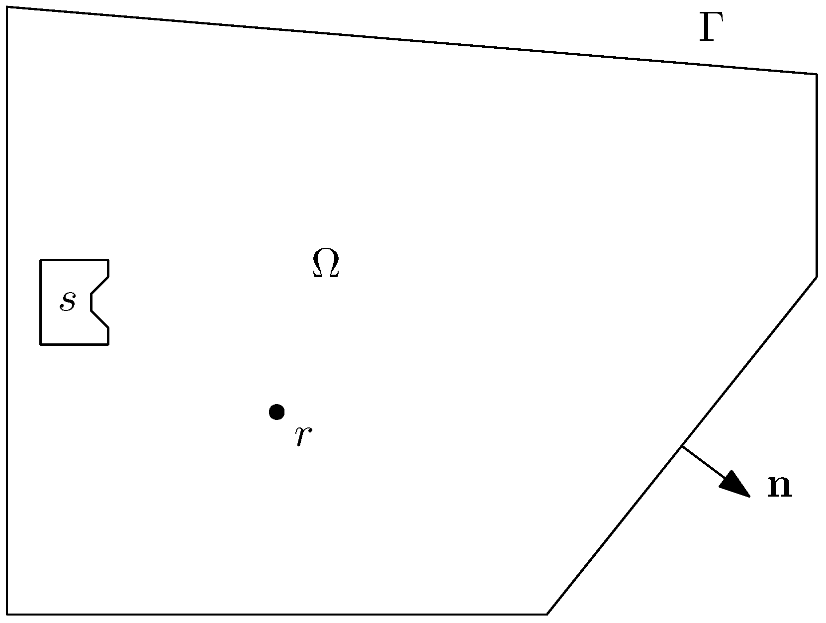
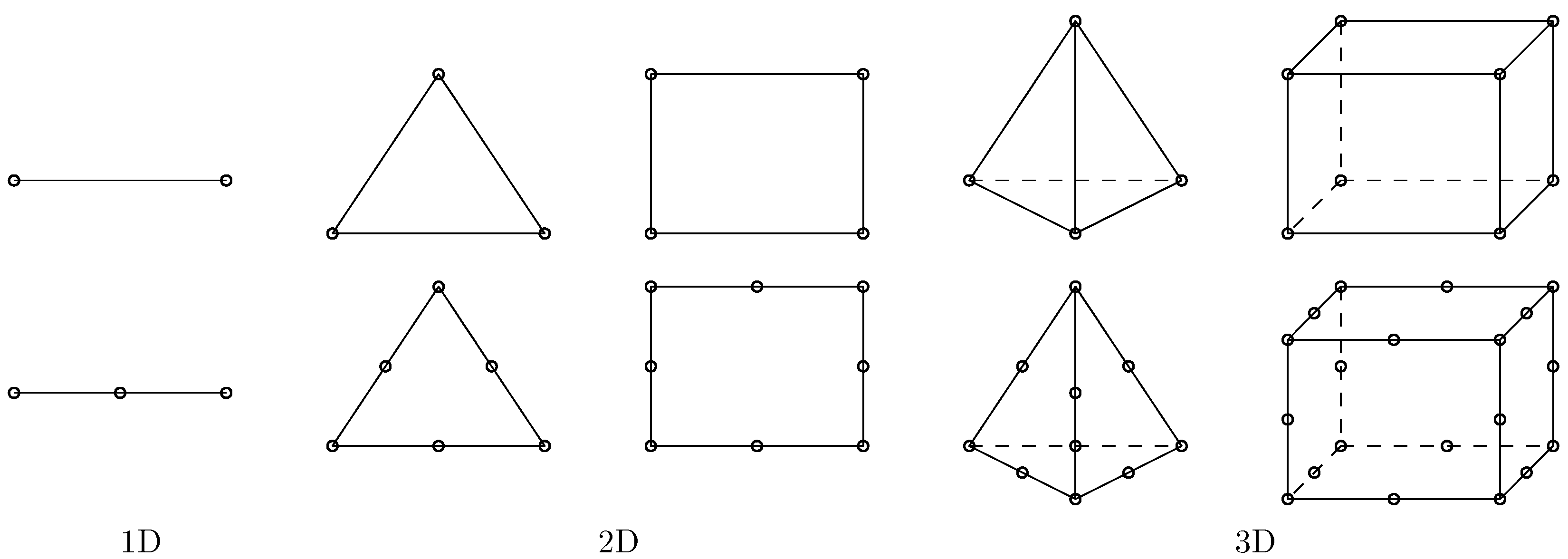
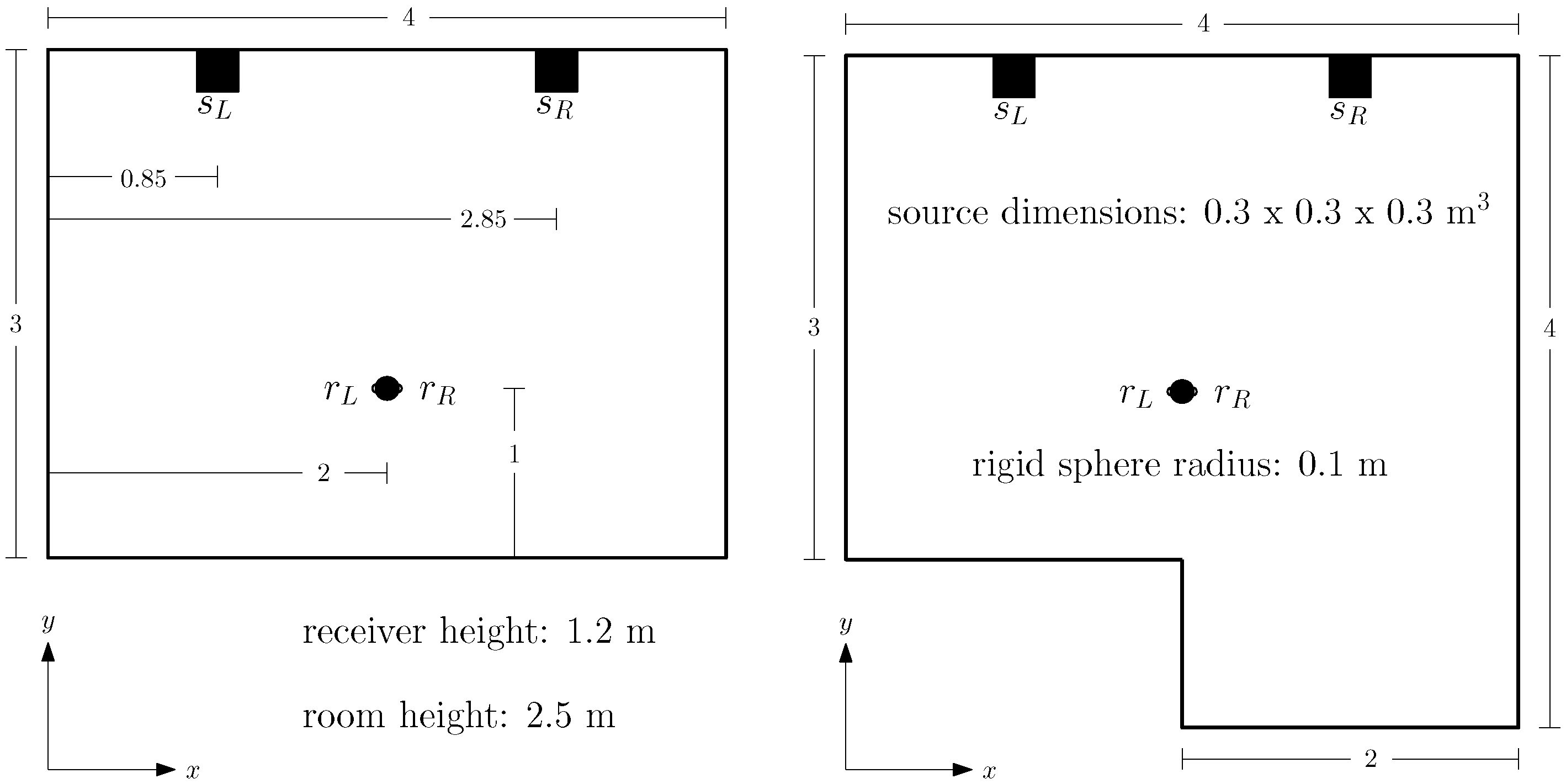
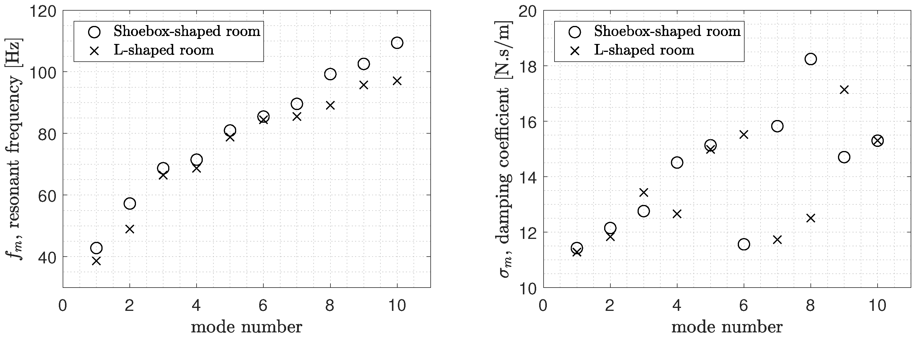
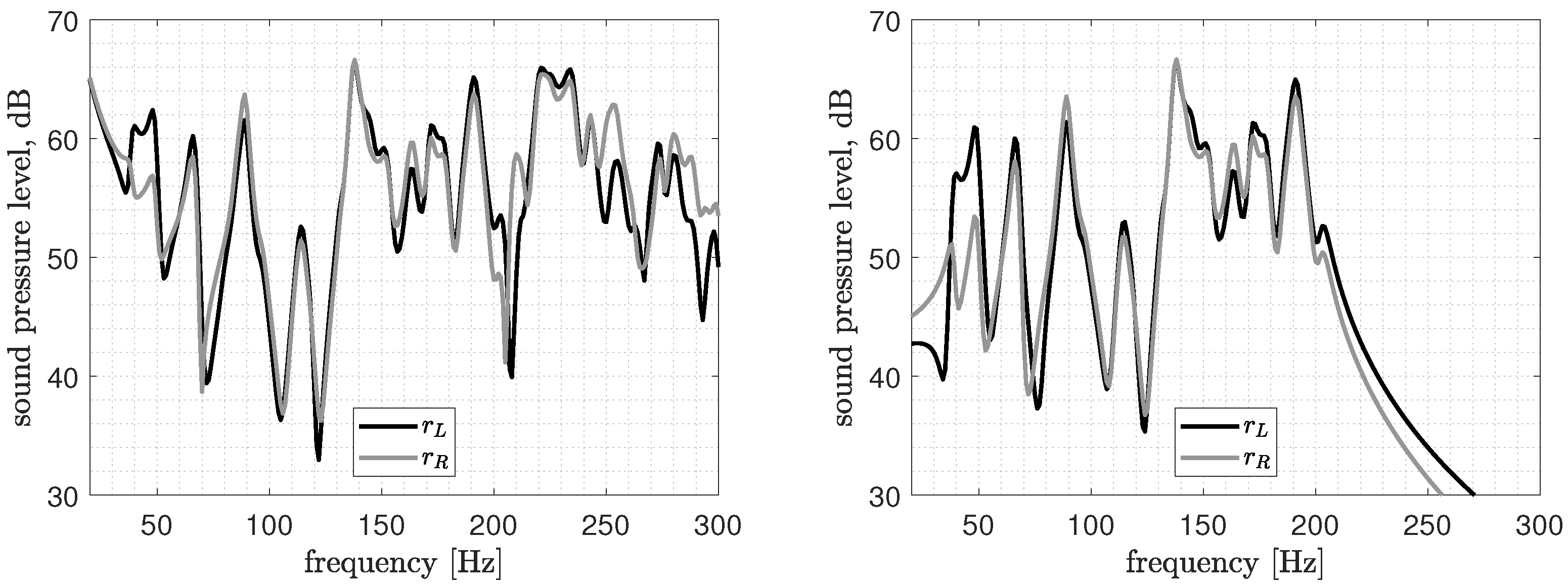
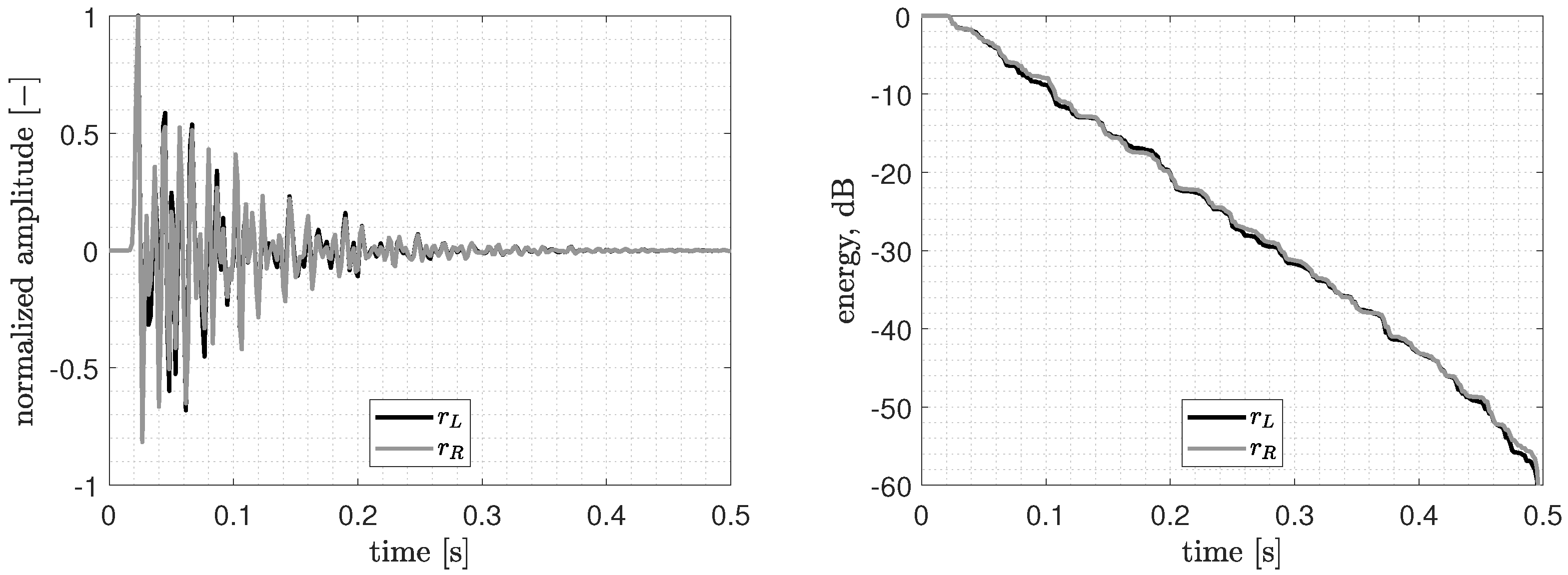
Table 1.
Natural frequencies of a rigid-walled rectangular room, with relative error.
| Exact [Hz] | FEM, tet. [Hz] | Error, tet. [%] | FEM, hex. [Hz] | Error, hex. [%] | |||
|---|---|---|---|---|---|---|---|
| 1 | 0 | 0 | 42.8750 | 42.8757 | 0.0016 | 42.8772 | 0.0051 |
| 0 | 1 | 0 | 57.1667 | 57.1693 | 0.0046 | 57.1727 | 0.0106 |
| 0 | 0 | 1 | 68.6000 | 68.6056 | 0.0082 | 68.6176 | 0.0256 |
| 1 | 1 | 0 | 71.4583 | 71.4668 | 0.0119 | 71.4645 | 0.0086 |
| 1 | 0 | 1 | 80.8964 | 80.9099 | 0.0166 | 80.9125 | 0.0199 |
| 2 | 0 | 0 | 85.7500 | 85.7707 | 0.0241 | 85.8178 | 0.0790 |
| 0 | 1 | 1 | 89.2972 | 89.3203 | 0.0258 | 89.3146 | 0.0195 |
| 1 | 1 | 1 | 99.0568 | 99.0941 | 0.0377 | 99.0734 | 0.0168 |
| 2 | 1 | 0 | 103.0587 | 103.1089 | 0.0487 | 103.1184 | 0.0580 |
| 2 | 0 | 1 | 109.8136 | 109.8829 | 0.0631 | 109.8775 | 0.0582 |
Disclaimer/Publisher’s Note: The statements, opinions and data contained in all publications are solely those of the individual author(s) and contributor(s) and not of MDPI and/or the editor(s). MDPI and/or the editor(s) disclaim responsibility for any injury to people or property resulting from any ideas, methods, instructions or products referred to in the content. |
© 2023 by the author. Licensee MDPI, Basel, Switzerland. This article is an open access article distributed under the terms and conditions of the Creative Commons Attribution (CC BY) license (https://creativecommons.org/licenses/by/4.0/).
Share and Cite
MDPI and ACS Style
Prinn, A.G. A Review of Finite Element Methods for Room Acoustics. Acoustics 2023, 5, 367-395. https://doi.org/10.3390/acoustics5020022
AMA Style
Prinn AG. A Review of Finite Element Methods for Room Acoustics. Acoustics. 2023; 5(2):367-395. https://doi.org/10.3390/acoustics5020022
Chicago/Turabian StylePrinn, Albert G. 2023. "A Review of Finite Element Methods for Room Acoustics" Acoustics 5, no. 2: 367-395. https://doi.org/10.3390/acoustics5020022