An Iterative Ray Tracing Algorithm to Increase Simulation Speed While Maintaining Overall Precision

Abstract

Ray tracing is a frequently used method for acoustic simulations, valued for its calculation speed and ease of use. Although it is fast, there are no fully ray tracing-based real-time simulation methods or engines. Under real-time restrictions, ray tracing simulations lose precision and the variance inherent in the random simulation method has too much impact on the outcome. In this paper, an algorithm called iterative ray tracing is presented that reduces the negative effects of real-time restrictions by iteratively improving the initial calculation and increasing the precision over time. In addition, new estimates of the expected value and variance of ray tracing simulations are presented and used to show the iteration steps in the new algorithm reduce variance, while maintaining the expected value. Simulations using iterative ray tracing are compared to measurements and simulations using the classical ray tracing method, and it is shown that iterative ray tracing can be used to improve precision over time. Although more testing is needed, iterative ray tracing can be used to extend most ray tracing algorithms, in order to decrease the adverse effects of real-time restrictions.

1. Introduction

Ray tracing is one of the most common methods of acoustic simulations [1] and is used in popular commercial acoustic simulation software [2,3,4]. Among its advantages are its relatively low computational load and its close relationship to geometrical acoustic (GA) models for sound propagation [1,5,6]. The relatively low computational load means that ray tracing is a good candidate for acoustic simulations in virtual reality (VR) and other real-time applications. Additionally, acoustic ray tracing can be used to unlock the extreme computational capabilities of modern Graphics Processing Units (GPUs) for the purpose of acoustic simulations [7,8]. The ray tracer used in this study is implemented to run on the GPU.

Today, there exists a range of acoustic simulation software aimed at VR and acoustically immersive experiences. The most precise simulation tools achieve their accuracy by solving the wave equation for low frequencies, but cannot be considered fully real-time, as they rely on computing at least parts of the acoustic response in advance [9,10]. On the other hand, some tools aimed primarily at entertainment purposes, such as video games, can be very fast, but are found to be of questionable physical accuracy [11]. In between these extremes, there are at least two applications relying on geometrical acoustics that are capable of real-time simulation. One is developed at the Technical University of Aachen (RWTH Aachen), and called Room Acoustics for Virtual Environments (RAVEN) [12]. It implements image source, ray tracing, and radiosity techniques. A second example is EVERTims [13], which is an open-source solution that combines an image sources with a statistical model for the late reverberation. Image source modelling is computationally efficient if a low order of image sources is used, which explains their prevalence in real-time modelling techniques. In EVERTims, the order of image sources is increased over time, thus refining the simulation data. As of yet, there is no real-time acoustic simulation software relying only on ray tracing, despite its popularity as an element of room acoustic simulation software [2,3].

If an acoustic application is to be perceptually real-time, the simulated sound field must respond to changes in the virtual environment sufficiently fast. There is no firm consensus on what should be considered “sufficiently fast”, but values in the range of 20–60 ms are called interactive in the literature [13,14]. The actual time limit depends on the actions of the listener and their attention, and a hard bound is, thus, hard to define. Within this time limit, the sound field must be updated to account for any changes in the environment. Depending on what these changes entail, the sound field update may consist only of impulse response filtering or the calculation of a completely new simulation [12]. The variations in time requirements indicate that there is a need for more adaptive simulation strategies.

Ray tracing is a prevalent room acoustic simulation tool, and the term defines both the model for sound propagation (geometrical acoustics) and the calculation method. The sound field is modelled as a set of plane waves, and typically only the energy content of the waves are considered [1,5]. With these assumptions, the sound field can be described as an infinite set of energy particles whose behavior is well-defined. This model for the sound field is called geometrical acoustics [6], and in the case of ray tracing, the acoustic field is estimated by Monte Carlo sampling of the energy particles (or rays) [15].

Monte Carlo methods are a class of simulation methods that rely on random sampling to calculate something that may be deterministic in nature. In the case of room acoustic simulations, the impulse response is defined by the wave equation and the space under consideration and is, thus, deterministic. It is estimated using random samples of energy particles and their paths. In practice, this means calculating the potential propagation paths for a large set of rays and determining their energy levels over time. As the rays intersect the position of the sound receiver, their energy is recorded and added to an estimate of the energetic impulse response. By sampling a large number of random ray paths, the deterministic impulse response can be estimated. Frequently, the impulse response is estimated in a given subset of positions, leading to a spatial discretization.

Although the impulse response is deterministic, the ray tracing simulation method itself is random. Consequently, the simulation outcome can be described by its statistical properties. The expected value of a simulation is the energetic impulse response defined by the geometrical acoustics model. The variance of the simulation outcome describes how much it may differ between calculations, and it can be used to gauge how accurate the calculation is. As is typical for Monte Carlo simulation methods, the expected value is independent of the number of samples whereas the variance decreases as the number of samples increase [16]. Since the variance should be minimized, it is often desirable to use as many rays as possible. However, the higher the number of rays, the higher the computational load and the longer the simulation time. Although the expected value and variance of ray tracing simulations typically cannot be calculated outright, accurate estimates provide insight into the simulation tool itself and can be used as a tool to evaluate simulation parameters, such as the number of rays used.

The lack of a real-time ray tracing option for acoustic simulations, despite its popularity, shows that there is a need for algorithms that allow for faster calculation. On the other hand, the simulation accuracy and precision should be maintained as far as possible, and it has been noted that the real-time limitations vary depending on the situation. A more flexible ray tracing simulation algorithm can be used to fill in both of these gaps.

In this paper, a ray tracing algorithm is presented, which allows for greater flexibility in finding the balance between simulation speed and precision. The algorithm, called Iterative ray tracing, can mitigate the issues caused by small sample sizes in ray tracing simulations when speed cannot be compromised with. It iteratively improves the simulation result until maximum precision is reached. The algorithm itself is easy to combine with other methods for improving the performance of ray tracers.

The algorithm is statistically equivalent to classical ray tracing. This is shown by developing a novel theoretical estimate of the expected value and variance of the energetic impulse response produced by ray tracing under diffused conditions. These estimates improve on earlier versions [14] by fully accounting for the randomness involved in ray tracing, and are compared to results from real simulations to ensure that they are accurate.

The following sections presents and explains iterative ray tracing, as well as formulates the novel estimates of the expected value and variance. From this foundation, the accuracy of the estimates are shown, and the functionality of the algorithm is demonstrated. This is followed by a brief discussion and conclusion.

2. Iterative Ray Tracing: Introduction

In real time acoustic simulation, the sound field presented to the listener should adapt to changes in the environment sufficiently fast that no delay can be perceived. When the listener, or user, is moving quickly through the simulated space or interacting with the environment in acoustically relevant ways (e.g., making noise, changing the environment by opening doors or similar), the real time requirement can be very restrictive. On the other hand, the user may, at times, refrain from interacting at all with the environment, instead remaining in one place and perceiving the surrounding space. In such situations, the time limit becomes almost irrelevant. Iterative ray tracing aims at improving the tools for finding a balance between these two extremes.

In the context of ray tracing, restrictive time limits impact the number of rays that can be used in the simulation. Reducing the number of rays does not change the expected outcome of the simulation, but it can increase variance to the point where the result is not usable. When the time limit imposes an upper bound on the number of rays that negatively affects the reliability of the simulation result, while not rendering it unusable, a possible solution is to iteratively improve the simulation result. In this way, the simulation can offer excellent precision, while still generating simulation results quickly enough to comply with real-time restriction [13]. This is the idea behind iterative ray tracing.

The calculated impulse response can be iteratively improved in cases when the simulated space has not changed since the last time frame. In other cases, the impulse response is no longer accurate and should be discarded. In the context of ray tracing, an intuitive way of improving the simulated impulse response is by increasing the number of rays. In iterative ray tracing, this is achieved by adding the results from a new ray tracing simulation to the existing, still accurate, impulse response. When the ray tracing simulations are configured in the right way, this is statistically equivalent to performing one single ray tracing simulation with a number of rays equal to the sums of the two separate simulations.

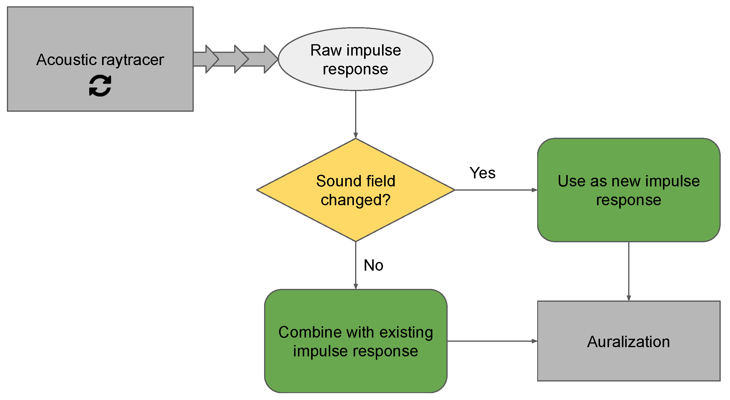
A flowchart illustrating the algorithm is shown in Figure 1. The ray tracing and auralization frameworks are presented as grey boxes, and their specific implementations are not considered. In this algorithm, the ray tracing engine is assumed to continuously produce impulse responses. New impulse responses (grey oval) are passed to the iterative algorithm, which is responsible for determining what to do next (yellow rhombus). If the acoustic field has changed significantly since the last frame, the newly produced impulse response is passed directly to auralization. If it has not, it is combined with the existing impulse response which may, in turn, consist of the result of multiple previous calculations, and then it is passed to the auralization engine. The combination of impulse responses is a central part of the iterative ray tracing algorithm. The conditions under which it can be performed and how it should be implemented are described in Section 3.2.

The iterative algorithm is responsive to the events in the environment, in that speed is prioritized when needed and higher quality calculations are provided when possible. In general, when a fully new calculation is performed, it coincides with some significant event in the environment, which, in turn, may distract the listener from possible momentary acoustic variations, due to sample size [17]. On the other hand, when a listener is stationary and inactive, the sound simulation is reliable and realistic.

When implementing this algorithm, a central aspect is determining the criteria for when a new simulation is needed. When particular events occur, such as a door opening or closing, it can be straightforward to determine whether it has occurred and the simulation should be updated. In many cases, such as the user moving to a new location, the situation is less clear. Typically, a human standing still is not entirely still, but makes very small movements, due to both breathing and heart beats. Such movements should not lead to the previous simulation being discarded, as they do not cause audible changes to the sound field. On the other hand, if the simulation is only updated when audible changes occur, the updates are naturally audible, rather than imperceptible.

In practice, this leads to a spatial discretization. Its resolution depends on how acoustically homogenous the simulated space is. The Nyquist–Shannon sampling theorem suggests a spatial resolution of about 4 cm, given a maximum frequency of 4 kHz, but research findings suggest that the human hearing’s spatial resolution for room acoustic variations is less fine [18,19]. Accurate estimates of the appropriate spatial resolution are yet to be determined, but are likely to be on the order of 20–75 cm. The spatial discretization can be based on the distance to the most recently calculated impulse response.

In the following section, it is shown that the iterative ray tracing algorithm can be implemented such that it has the same expected value and variance as the classical algorithm.

3. Expected Value and Variance of Ray Tracing Simulations

Iterative ray tracing relies on the fact that separate ray tracing simulations can be combined to reduce variance while maintaining the expected value. By studying the expected value and variance of impulse responses generated by ray tracing, as well as their sums, this prerequisite can be evaluated. While it is not possible to derive a general closed-form expression, estimates can be formed by making some strong assumptions on the distribution of sound energy in the simulated space. In this section, such estimates are formed for both classical and iterative ray tracing. The discussion in this section is applicable to ray tracers in general and is specific to the iterative algorithm only when specified.

While the estimates of the expected value and variance of ray tracing simulations exist [14], they do not take the full stochastic nature of Monte Carlo simulations into account. This leads to a significant simplification of the expressions and associated calculations, but may also have a significant impact on the accuracy of the estimates. The estimates derived in this paper do not rely on such assumptions and are, consequently, more formally accurate. They may, therefore, lead to an increased understanding of the behavior of ray tracing simulations and may be used to evaluate the accuracy of the earlier, simplified expressions. The derived expressions are compared both to earlier estimates and to real simulation outcomes, to evaluate their accuracy.

Theoretical estimates of the expected value and variance of a ray tracing simulations are a useful tool in learning more about ray tracing simulations, but can, in general, not be used as a tool to study the real sound field. In particular, the estimated variance only relates to the simulation outcome and not the real sound field in any way. Since ray tracing is a Monte Carlo simulation method, the expected result of a ray tracing simulation is the impulse response predicted by the GA model. However, the theoretical estimate of the expected value of the impulse response relies on strict assumptions on the sound field, which are generally never fulfilled in real spaces. Consequently, the expression for the expected value should not be used as a substitute for a real ray tracing simulation. In this paper, it is used to compare the expected value of different simulation configurations.

The most central assumption in the derivation of the estimates below is the assumption of diffuseness. In this context, a diffused sound field is a sound field which is described entirely by its statistical properties. Real sound fields can be more or less diffused, where a more diffused sound field has a more even distribution of sound energy with little to no net flow of acoustic energy. In less diffused sound fields, there is at least some net flow of acoustic energy caused by properties of the surrounding space itself. When making general estimates of the sound energy, no information is known about the space and the assumption of diffuseness becomes a best-guess of the distribution of sound energy. Since the expressions derived in this paper should be generally applicable, it is assumed that the sound field is sufficiently diffused to be described by its statistical properties.

Under some circumstances, the assumption of diffuseness is not fulfilled. In particular, in the very early parts of the impulse response, the sound field is not diffused. Immediately when a sound impulse is emitted, there is a concentration of sound energy at that position, and the sound field cannot be described as diffused before some amount of diffusion has occurred. Other factors that affect the level of diffuseness are the simulated space and the amount of surface scattering. In general, very geometrically regular spaces, low surface scattering, or very unevenly distributed absorption can lead to a sound field that is highly non-diffused. In these cases, the estimates derived in this section are less accurate.

Finally, some comments are made regarding frequency dependence and scattering and absorption parameters. In general, the behavior of low and high frequency acoustical waves differ significantly and this is typically implemented in ray tracers by frequency-dependent surface absorption and scattering. In the derivation of the expected value and variance, however, it is assumed that the sound field is diffused for all frequencies. A consequence of this is that the scattering parameter, which would normally relate to the amount of diffuseness in the sound field; however, is not considered in the calculations below. In terms of the absorption coefficient, the assumption of diffuseness ensures that an average absorption coefficient for the walls of the enclosure is adequate. It is, consequently, assumed to be constant for all surfaces in the sequel. In terms of frequency dependence, the theoretical estimates derived in this paper, thus, only takes it into account in the definition of surface and air absorption coefficients.

3.1. Classical Ray Tracing Simulation: Expected Value and Variance

In this section, an estimate is derived for the expected value and variance of the energetic impulse response found by ray tracing simulation. The energetic impulse is discretized in the time domain and contains the energy detected at the listener position for each time step. The expected value and variance is, consequently, also defined for each time frame. It is assumed that the ray tracing simulations take place in a closed volume, where acoustic energy is lost only by surface or air absorption. It is further assumed that surface absorption is constant and non-zero, to ensure that the acoustic energy decays over time.

We find that in time step k, the energy detected $E_k$ can be described as

$$\begin{array}{c}\hfill E_k=\sum _{j=1}^N{i}_{j,k}{e}_{j,k},\end{array}$$

(1)

where $i_{j,k}$ is the number of times ray j intersects the detector in time interval k, and $e_{j,k}$ is the energy of ray j in time interval k. N is the total number of rays in the simulation. Note that the energy of each ray is assumed to be constant during the full time step. This assumption is acceptable if the time step $\Delta t$ is sufficiently small.

If all rays are generated the same way, with constant energy and a randomly generated direction, they have identical distribution, and the expected values $\mathbb{E}\left[i_{j,k}\right]$ and $\mathbb{E}\left[e_{j,k}\right]$ are constant for all values j. Furthermore, it is assumed that $i_{j,k}$ and $e_{j,k}$ are mutually independent. This is true if the energy of each ray is unrelated to how likely it is to be found close to the detector. For example, this assumption would not necessarily hold if the detector is placed close to several absorptive surfaces, as rays close to absorbers are more likely to have lower energy. Since we consider the sound field to be diffuse; however, we can assume that $i_{j,k}$ and $e_{j,k}$ are independent. We can then write the expected value $\mathbb{E}\left[E_k\right]$

$$\mathbb{E}\left[E_k\right]=\mathbb{E}\left[\sum _{j=1}^N{i}_{j,k}{e}_{j,k}\right]=\sum _{j=1}^N\mathbb{E}\left[i_{j,k}\right]\mathbb{E}\left[e_{j,k}\right]=N\mathbb{E}\left[i_{j,k}\right]\mathbb{E}\left[e_{j,k}\right].$$

(2)

The number of times a given ray intersects the detector in a given time interval, $i_{j,k}$, is Poisson distributed. In fact, $i_{j,k}\in \mathrm{Po}\left(\overline{n}\frac{S_d}{S}\Delta t\right)$, where $S_d$ is the surface area of the detector (given by $4\pi r_d^2$ if it is modelled as a sphere with radius $r_d$), S is the total surface area of the modelled space, and $\overline{n}$ is the average rate of reflection for a ray. In a diffused field, $\overline{n}=\frac{cS}{4V}$, where V is given by the volume of the space and c is the speed of sound [6]. This yields, for expected value $\mathbb{E}$ and variance $\mathbb{V}$,

$$\mathbb{E}\left[i_{j,k}\right]=\mathbb{V}\left[i_{j,k}\right]=\overline{n}\frac{S_d}{S}\Delta t=\overline{i},$$

(3)

where the detection rate $\overline{i}$ has been introduced to simplify the expressions. It is the expected number of times a ray hits the detector in a single time step. Note that $\overline{i}$ is independent of j, as has already been discussed, but also independent of time k. In most ray tracing simulations, rays are eventually terminated and no longer detectable once their energy falls below some threshold. The detection rate should, thus, tend to zero over time. In the later parts of the impulse response, assuming a constant detection rate $\overline{i}$ may lead to an inflated estimate of the detected energy, as compared to the results of the simulation. If the energy threshold for termination is set sufficiently low in the simulation, this does not have a significant impact on the accuracy of the estimate.

The energy of each ray, $e_{j,k}$, decreases over time as energy is absorbed from surface reflections and air absorption. The latter is assumed to be deterministic, whereas energy absorbed from surface reflections depend on the number of reflections a given ray has undergone. It is found that

$$e_{j,k}=e_0{\mathrm{e}}^{-\gamma ck\Delta t}{\left(1-\alpha \right)}^{m_{j,k}}=e_0{a}_k{\left(1-\alpha \right)}^{m_{j,k}},$$

(4)

where $e_0$ is the initial energy of an emitted ray, $\alpha$ is the absorption parameter of the walls of the enclosure (here assumed to be constant), ${\mathrm{e}}^{-\gamma ck\Delta t}=a_k$ accounts for air absorption, and $m_{j,k}$ is the number of surface reflections ray j has undergone at time step k. Since the number of reflections depends on the random ray path, it is stochastic and the energy is also stochastic. The number of reflections a ray has undergone at a given time is a Poisson process and $m_{j,k}\in \mathrm{Po}\left(\overline{n}k\Delta t\right)$. Accordingly, $\mathbb{E}\left[m_{j,k}\right]=\mathbb{V}\left[m_{j,k}\right]=\overline{n}k\Delta t={\overline{m}}_k$, where the expected number of reflections a given ray has undergone at time k, ${\overline{m}}_k$, has been introduced. This number increases as k increases, but is, again, independent of j.

The ray energy $e_{j,k}$ is stochastic, as it depends on the path of the given ray, which is randomly generated. However, in a completely diffused sound field, the rays would be evenly distributed in space and have equal energy. It is, thus, possible to assume that the energy decay of each ray is deterministic and determined by models for diffused sound decay in enclosures, so that $m_{j,k}\triangleq {\overline{m}}_k$ and $\mathbb{V}\left[e_{j,k}\right]=0$. With this assumption, the mathematical operations become significantly more simple and compact, and it has been used in previous derivations [14]. In this paper, the stochastic nature of the energy levels is, instead, dealt with by introducing a Taylor expansion. Either of these solutions are approximations that introduce some level of uncertainty.

As mentioned, the ray energy is a function of a stochastic variable in our model, $e_{j,k}=e_{j,k}\left(m_{j,k}\right)$. An estimate of $\mathbb{E}\left[e_{j,k}\right]$ can be formed by using a Taylor expansion about the expected value of $m_{j,k}$. The general expression for the second order Taylor expansion of the expected value of a function of a stochastic variable $\mathbb{E}\left[f\left(x\right)\right]$ about the expected value of $x=\mu$ is:

$$\mathbb{E}\left[f\left(x\right)\right]\approx \mathbb{E}\left[f\left(\mu \right)+f^{\prime }\left(\mu \right)\left(x-\mu \right)+\frac{1}{2}{f}^{″}\left(\mu \right){\left(x-\mu \right)}^2\right]=f\left(\mu \right)+\frac{1}{2}{f}^{″}\left(\mu \right)\mathbb{V}\left[x\right],$$

(5)

using the fact that $\mathbb{E}\left[x-\mu \right]=0$ and $\mathbb{V}\left[x\right]=\mathbb{E}\left[{\left(x-\mu \right)}^2\right]$.

Inserting $e_{j,k}=e_{j,k}\left(m_{j,k}\right)$ for f and using $\mathbb{E}\left[m_{j,k}\right]=\mathbb{V}\left[m_{j,k}\right]={\overline{m}}_k$, we obtain

$$\mathbb{E}\left[e_{j,k}\right]\approx e_0{a}_k{\left(1-\alpha \right)}^{{\overline{m}}_k}+\frac{1}{2}{e}_0{a}_k{\left(1-\alpha \right)}^{{\overline{m}}_k}{ln}^2\left(1-\alpha \right){\overline{m}}_k.$$

(6)

We define the dimensionless constant $\widehat{\alpha }=ln\left(1-\alpha \right)$ and insert Equations (3) and (6) into Equation (2), obtaining

$$\mathbb{E}\left[E_k\right]=N\mathbb{E}\left[i_{j,k}\right]\mathbb{E}\left[e_{j,k}\right]\approx N{e}_0{a}_k\overline{i}\left({\mathrm{e}}^{\widehat{\alpha }{\overline{m}}_k}+\frac{{\mathrm{e}}^{\widehat{\alpha }{\overline{m}}_k}}{2}{\widehat{\alpha }}^2{\overline{m}}_k\right).$$

(7)

This is an estimate of the expected energy in the energetic impulse response produced by a ray tracer. If $N{e}_0=1\iff e_0=\frac{1}{N}$, the total energy emitted in the impulse is 1, and the impulse response is normalized. For this case, we set $\mathbb{E}\left[E_k\right]={\mathbf{E}}_k$. When the initial ray energy is determined this way, the expected value is independent of the number of rays; additionally, the impulse response neither amplifies nor diminishes sounds emitted in the space.

The variance of the energetic impulse response can be estimated using a Taylor expansion in a similar way. Firstly, we note that its variance can be calculated by

$$\mathbb{V}\left[E_k\right]=\mathbb{V}\left[\sum _{j=1}^N{i}_{j,k}{e}_{j,k}\right]=N\left(\mathbb{V}\left[i_{j,k}\right]\mathbb{V}\left[e_{j,k}\right]+\mathbb{V}\left[i_{j,k}\right]{\mathbb{E}}^2\left[e_{j,k}\right]+\mathbb{V}\left[e_{j,k}\right]{\mathbb{E}}^2\left[i_{j,k}\right]\right),$$

(8)

if we assume that $\mathbb{COV}\left[E_k,E_l\right]$ for all $k\ne l$, or that they are mutually independent. Since the distribution of $i_{j,k}$ is known from Equation (3), we find that $\mathbb{V}\left[i_{j,k}\right]=\overline{i}$, ${\mathbb{E}}^2\left[i_{j,k}\right]={\overline{i}}^2$

Using our earlier approximation of $\mathbb{E}\left[e_{j,k}\right]$, we determine

$${\mathbb{E}}^2\left[e_{j,k}\right]\approx e_0^2{a}_k^2{\mathrm{e}}^{\widehat{\alpha }2{\overline{m}}_k}\left(1+{\widehat{\alpha }}^2{\overline{m}}_k+\frac{1}{4}{\widehat{\alpha }}^4{\overline{m}}_k^2\right).$$

(9)

In addition, an estimate of $\mathbb{E}\left[e_{j,k}^2\right]$ needs to be constructed. This is achieved by Taylor expansion,

$$\begin{array}{cc}\hfill \mathbb{E}\left[f^2\left(x\right)\right]& \approx \mathbb{E}\left[f^2\left(\mu \right)+2f\left(\mu \right)f^{\prime }\left(\mu \right)(x-\mu )+2\frac{{\left(x-\mu \right)}^2}{2}\left(f^{\prime 2}\left(\mu \right)+f\left(\mu \right)f^{″}\left(\mu \right)\right)\right]\hfill \\ \hfill & =f^2\left(\mu \right)+\left(f^{\prime 2}\left(\mu \right)+f\left(\mu \right)f^{″}\left(\mu \right)\right)\mathbb{V}\left[x\right].\hfill \end{array}$$

(10)

Using $e_{j,k}=e_{j,k}\left(m_{j,k}\right)$, $\mathbb{E}\left[m_{j,k}\right]=\mathbb{V}\left[m_{j,k}\right]={\overline{m}}_k$ and Equation (9), an estimate of the variance $\mathbb{V}\left[e_{j,k}\right]$ is found as

$$\mathbb{V}\left[e_{j,k}\right]\approx e_0^2{a}_k^2{\mathrm{e}}^{\widehat{\alpha }2{\overline{m}}_k}\left({\overline{m}}_k{\widehat{\alpha }}^2-\frac{{\widehat{\alpha }}^4}{4}{\overline{m}}_k^2\right)$$

(11)

Finally, Equations (9) and (11) are inserted into Equation (8) to arrive at an estimate for $\mathbb{V}\left[E_k\right]$:

$$\begin{array}{cc}\hfill \mathbb{V}\left[E_k\right]& =N\left(\mathbb{V}\left[i_{j,k}\right]\mathbb{V}\left[e_{j,k}\right]+\mathbb{V}\left[i_{j,k}\right]{\mathbb{E}}^2\left[e_{j,k}\right]+\mathbb{V}\left[e_{j,k}\right]{\mathbb{E}}^2\left[i_{j,k}\right]\right)\hfill \\ \hfill & \approx N{e}_0^2{a}_k^2{\mathrm{e}}^{\widehat{\alpha }2{\overline{m}}_k}\overline{i}\left(1+2{\overline{m}}_k{\widehat{\alpha }}^2+\overline{i}{\overline{m}}_k{\widehat{\alpha }}^2-\frac{{\widehat{\alpha }}^4}{4}{\overline{m}}_k^2\overline{i}\right)\hfill \end{array}$$

(12)

This is an estimate of the variance of the energetic impulse response produced by ray tracing simulations. Reviewing the expression, it seems that the total variance increases as the number of rays N increases. If we, instead, consider the normalized impulse response ${\mathbf{E}}_k$, the case when the product $N{e}_0=1\iff e_0=\frac{1}{N}$, we find that

$$\mathbb{V}\left[{\mathbf{E}}_k\right]=\frac{1}{N}{a}_k^2{\mathrm{e}}^{\widehat{\alpha }2{\overline{m}}_k}\overline{i}\left(1+2{\overline{m}}_k{\widehat{\alpha }}^2+\overline{i}{\overline{m}}_k{\widehat{\alpha }}^2-\frac{{\widehat{\alpha }}^4}{4}{\overline{m}}_k^2\overline{i}\right)=\frac{1}{N}{V}_k,$$

(13)

where $V_k$ has been introduced for the factor of the variance that is independent of the number of rays. The total variance, thus, decreases as the number of rays increase.

In conclusion, an estimate for the expected value and variance of the outcome of acoustic ray tracing simulations has been derived, as shown in Equations (7) and (12). When the initial ray energy $e_0$ is set, so that $N{e}_0=1$, the expected value is independent of and the variance is inversely proportional to the number of rays.

In order to show that the iterative ray tracing algorithm can be used to further decrease variance, while maintaining the expected value, it is reviewed in the following section.

3.2. Iterative Ray Tracing: Expected Value and Variance

In this section, the estimates of the expected value and variance of the iterative ray tracing algorithm are derived. From those estimates, the method for combining the impulse responses from distinct ray tracing simulations is more closely defined to ensure that the iterative ray tracing algorithm has the desired expected value and variance. It is shown that, using the method presented in this paper, the iterative ray tracing algorithm has the same expected value as the classical algorithm. Initially, only the combination of two simulations are considered. The results are then generalized to multiple simulations.

Consider the sum of two separate simulations, each consistent with the expression for the energetic impulse response in Equation (1). In general, the variables related to the secondary simulations are denoted as ${·}^{*}$, and variables from the iterative algorithm are marked with an I. The expected value for the detected energy in each time step using the iterative algorithm, $E_k^I$, then becomes

$$E_k^I=\sum _{j=1}^N{i}_{j,k}{e}_{j,k}+\sum _{l=1}^{N^{*}}{i}_{l,k}^{*}{e}_{l,k}^{*}.$$

(14)

For the expected value and variance, it is known that

$$\begin{array}{cc}\hfill \mathbb{E}\left[x+y\right]& =\mathbb{E}\left[x\right]+\mathbb{E}\left[y\right],\hfill \\ \hfill \mathbb{V}\left[x+y\right]& =\mathbb{V}\left[x\right]+\mathbb{V}\left[y\right]+2\mathbb{COV}\left[x,y\right],\hfill \end{array}$$

(15)

where $\mathbb{COV}$ denotes the covariance. Since the initial ray tracing step is generated randomly in the same way as the initial simulation, the expressions derived in Equations (7) and  (12) can be used to determine the expected value and variance of the secondary sum in Equation  (14). Regarding the covariance, it describes how the random variations in the two simulations are connected. When the two simulations are randomly and independently initialized, the covariance term can generally be discarded. It is, consequently, important to ensure that, for example, the same random seed or ray generation pattern is not used for both simulations.

We find that, using Equations (14), (7), and (12)

$$\begin{array}{cc}\hfill \mathbb{E}\left[E_k^I\right]\approx & N{e}_0{a}_k\overline{i}\left({\mathrm{e}}^{\widehat{\alpha }{\overline{m}}_k}+\frac{{\mathrm{e}}^{\widehat{\alpha }{\overline{m}}_k}}{2}{\widehat{\alpha }}^2{\overline{m}}_k\right)\hfill \\ \hfill & +N^{*}{e}_0^{*}{a}_k{\overline{i}}^{*}\left({\mathrm{e}}^{\widehat{\alpha }{\overline{m}}_k^{*}}+\frac{{\mathrm{e}}^{\widehat{\alpha }{\overline{m}}_k^{*}}}{2}{\widehat{\alpha }}^2{\overline{m}}_k^{*}\right),\hfill \end{array}$$

(16)

$$\begin{array}{cc}\hfill \mathbb{V}\left[E_k^I\right]\approx & N{e}_0^2{a}_k^2{\mathrm{e}}^{\widehat{\alpha }2{\overline{m}}_k}\overline{i}\left(1+2{\overline{m}}_k{\widehat{\alpha }}^2+\overline{i}{\overline{m}}_k{\widehat{\alpha }}^2-\frac{{\widehat{\alpha }}^4}{4}{\overline{m}}_k^2\overline{i}\right)\hfill \\ \hfill & +N^{*}{e}_0^{*2}{a}_k^2{\mathrm{e}}^{\widehat{\alpha }2{\overline{m}}_k^{*}}\overline{i}\left(1+2{\overline{m}}_k^{*}{\widehat{\alpha }}^2+{\overline{i}}^{*}{\overline{m}}_k^{*}{\widehat{\alpha }}^2-\frac{{\widehat{\alpha }}^4}{4}{\overline{m}}_k^{*2}{\overline{i}}^{*}\right).\hfill \end{array}$$

(17)

If the simulated space has not changed significantly between the two simulations, it can be assumed that $\overline{i}\approx {\overline{i}}^{*}$ and ${\overline{m}}_k\approx {\overline{m}}_k^{*}$. This mean that the expected number of times a given ray hits the detector $\overline{i}$ and the expected number of reflections a ray has undergone at time k, ${\overline{m}}_k$ is the same in the two simulations. Using this assumption, we can express Equations (16) and (17) as

$$\mathbb{E}\left[E_k^I\right]\approx \left(N{e}_0+N^{*}{e}_0^{*}\right)a_k\overline{i}\left({\mathrm{e}}^{\widehat{\alpha }{\overline{m}}_k}+\frac{{\mathrm{e}}^{\widehat{\alpha }{\overline{m}}_k}}{2}{\widehat{\alpha }}^2{\overline{m}}_k\right)=\left(N{e}_0+N^{*}{e}_0^{*}\right){\mathbf{E}}_k,$$

(18)

$$\begin{array}{c}\hfill \mathbb{V}\left[E_k^I\right]\approx \left(N{e}_0^2+N^{*}{e}_0^{*2}\right)a_k^2{\mathrm{e}}^{\widehat{\alpha }2{\overline{m}}_k}\overline{i}\left(1+2{\overline{m}}_k{\widehat{\alpha }}^2+\overline{i}{\overline{m}}_k{\widehat{\alpha }}^2-\frac{{\widehat{\alpha }}^4}{4}{\overline{m}}_k^2\overline{i}\right)=\left(N{e}_0^2+N^{*}{e}_0^{*2}\right)V_k,\end{array}$$

(19)

where ${\mathbf{E}}_k$, the expected value of the normalized impulse response and $V_k$, and the portion of the variance that is independent of the number of rays (see Equation (13)) has been reintroduced.

The results presented above can easily be generalized to the case where more than two simulations are used, and we find that for the $\nu$th iterative step,

$$\mathbb{E}\left[E_{k,\nu }\right]=\left(\sum _{\kappa =1}^{\nu }{N}_{\kappa }{e}_{0,\kappa }\right){\mathbf{E}}_k,$$

(20)

$$\mathbb{V}\left[E_{k,\nu }\right]=\left(\sum _{\kappa =1}^{\nu }{N}_{\kappa }{e}_{0,\kappa }^2\right)V_k.$$

(21)

In the case of a single simulation, the initial ray energy is typically set so that $N{e}_0=1$, as this produces an impulse response that is normal, in the sense that it does not artificially amplify or diminish sound energy. When this is the case, $\mathbb{E}\left[E_k\right]={\mathbf{E}}_k$. Since the iterative ray tracing algorithm should not change the expected outcome of the simulation, the resulting summed impulse response $E_{k,\nu }$ in Equation (20) must be normalized by $\sum N_{\kappa }{e}_{0,\kappa }$ or the total emitted energy in all simulations.

We find that

$$\mathbb{E}\left[\frac{1}{{\sum }_{\kappa =1}^{\nu }{N}_{\kappa }{e}_{0,\kappa }}{E}_{k,\nu }\right]=\frac{1}{{\sum }_{\kappa =1}^{\nu }{N}_{\kappa }{e}_{0,\kappa }}\mathbb{E}\left[E_{k,\nu }\right]={\mathbf{E}}_k.$$

(22)

Now, we consider the variance of the normalized iterative impulse response.

$$\mathbb{V}\left[\frac{1}{{\sum }_{\kappa =1}^{\nu }{N}_{\kappa }{e}_{0,\kappa }}{E}_{k,\nu }\right]=\frac{1}{{\sum }_{\kappa =1}^{\nu }{N}_{\kappa }^2{e}_{0,\kappa }^2}\mathbb{V}\left[E_{k,\nu }\right]=\frac{1}{{\sum }_{\kappa =1}^{\nu }{N}_{\kappa }^2{e}_{0,\kappa }^2}\sum _{\kappa =1}^{\nu }{N}_{\kappa }{e}_{0,\kappa }^2{V}_k.$$

(23)

The underlying theory behind iterative ray tracing comes from Monte Carlo simulation theory, which states that the simulation precision increases as the number of samples, or rays, increases. However, this relies on the samples being identically distributed. Consequently, the initial energy should be constant for all rays, $e_{0,\kappa }=e_0$. Inserting this into Equation (23) gives

$$\mathbb{V}\left[\frac{1}{{\sum }_{\kappa =1}^{\nu }{N}_{\kappa }{e}_{0,\kappa }}{E}_{k,\nu }\right]=\frac{1}{{\sum }_{\kappa =1}^{\nu }{N}_{\kappa }}{V}_k.$$

(24)

Here, the variance decreases by the total number of rays in all iteration steps. This is equivalent to the behavior in the classical algorithm and is the suggested method for this algorithm.

In conclusion, if multiple ray tracing simulations are run independently for the same space using the same initial ray energy, the sum of their results normalized by the total emitted energy has the same expected value and variance as a single ray tracing simulation using the total number of rays emitted in all simulations.

4. Method

In this section, the methods used to test the iterative ray tracing algorithm and the estimated expected value and variance are described. As a first step, the space used for digital simulations and measurements is described. The measurements are described, as well as the simulation setups used. Finally, the implementation of the ray tracer, post-processing of the results, and some timing tests are commented.

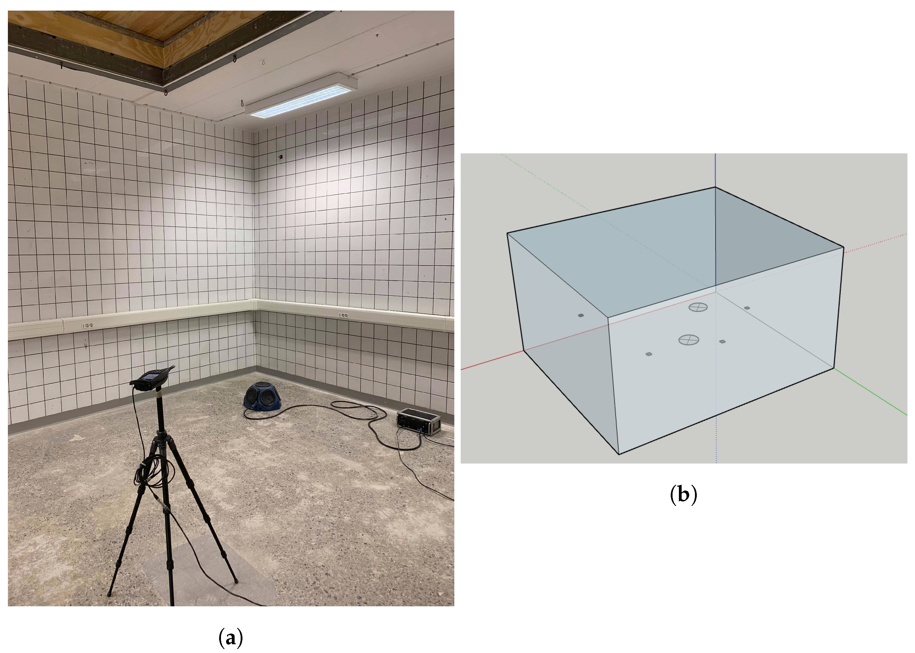
4.1. Measurement and Simulation Space

The space used for measurements and simulations was the lower chamber in the impact sound lab at the Division of Engineering acoustics, Lund University (see Figure 2). The space has an approximate volume of 95 m${}^3$ and a mid-frequency reverberation time of about 1.3 s. During the measurements, a suspended acoustic ceiling of porous absorbers was mounted in the center of the ceiling. This common acoustic treatment generally leads to a sound field with a net flow of acoustic energy towards the ceiling. This reduces the diffuseness in the sound field.

The space is rectangular, indicating that there should be strong and clear influences from eigenfrequencies in the low frequency range. Since ray tracers, in general, do not take resonance into account, the simulation results are expected to be relatively poor in the low frequency range. The Schroeder frequency can be used as a lower bound of the cut-off between these two cases, and it is found to be approximately 234 Hz [14]. In this project, especially the frequency bands centered on 125 Hz and 250 Hz are expected to be affected by resonances.

Acoustic impulse response measurements were obtained for validation of the ray tracer. Measurements were performed based on the international standards for room acoustic measurements [20] and have been previously described in 2021 [15]. An exponential sweep were used to obtain impulse response measurements. The measurements were performed using the open-source software REW version 5.19 (https://www.roomeqwizard.com/, accessed on 5 October 2022). A laptop with the software installed was connected to an Audio 8 DJ soundcard from Native instruments (Berlin, Germany) (https://www.native-instruments.com/en/, accessed on 5 October 2022), which connected to a Brüel & Kjær amplifier type 2734 (Hottinger Brüel & Kjær, Virum, Denmark) (https://www.bksv.com/en/transducers/acoustic/sound-sources/power-amplifier-2734, accessed on 29 August 2021). The amplifier fed the excitation signal to a dodecahedral loudspeaker. As a microphone, a Brüel & Kjær 2270 Sound Level Meter and Analyzer (Hottinger Brüel & Kjær, Virum, Denmark) (https://www.bksv.com/en/instruments/handheld/sound-level-meters/2270-series/type-2270-s, accessed on 5 October 2022) was used. A total of eight configurations were measured, two source positions and four listener positions, which are marked in Figure 2b. Due to technical and practical limitations, the sound source was located closer to the floor than what is prescribed in the standards.

4.2. Simulation Setups

Simulations were performed in the model space using both a classical ray tracer and using the iterative algorithm. Two main sets of simulations were performed, one to evaluate the theoretical estimates of the expected value and variance and one to evaluate the similarity between the classical and iterative algorithms. Both are described below.

When testing the estimates for expected value and variance, the surface absorption coefficient was constant across all frequency bands, but the air attenuation and scattering parameters were frequency dependent. The surface absorption was set uniformly to $\alpha =0.1$ across all surfaces and frequencies and air attenuation and scattering parameters are presented in

Table 1. Simulation parameters described for each octave band by frequency (f). s is the dimensionless surface scattering parameter, constant for all surfaces in the space. $\gamma$ is the air attenuation parameter, defined in m${}^{-1}$. Finally, the dimensionless absorption coefficients $\alpha$ are given for the surfaces in the model. Note that the surface absorption parameters were not used in the simulations designed to evaluate the estimates of expected value and variance. Surface scattering and absorption parameters are based on calibration from earlier research [15].

f(Hz)	s	$\mathit{\gamma }$(m${}^{-1}$)	$\mathit{\alpha }$, Walls	$\mathit{\alpha }$, Floor	$\mathit{\alpha }$, Ceiling Absorbers
125	0.01	0	0.0734	0.0596	0.25
250	0.13	0	0.056	0.0453	0.80
500	0.05	0.00064	0.0453	0.0453	0.95
1000	0.13	0.0015	0.04	0.045	0.95
2000	0.1	0.00208	0.045	0.045	0.95
4000	0.25	0.00532	0.045	0.045	0.95

. Air attenuation is set based on the environmental conditions of the measurement space during measurements, and the scattering parameters were set based on the results of earlier research [15]. Since the scattering parameter affects how diffused the simulated sound field is, their variations across the frequency range should lead to variations where frequency bands with higher scattering coefficients should match the theoretical results better.

Simulations were also used to examine the difference between the iterative and the classical ray tracing algorithms. In these simulations, surface absorption parameters varied across surfaces and frequency bands, shown in Table 1. Air attenuation and surface scattering parameters were identical to what was used in simulations for theory evaluation.

For both of the configurations described above, ray tracing simulations were performed using both the classical and the iterative algorithms. A total of eight configurations were simulated, two source positions and four listener positions (as shown in Figure 2b). In the classical ray tracer, 900,000 rays were used. In the iterative algorithm, each iteration used 9000 rays and there were 100 iterations. This results in a total of 900,000 rays contributing to the final impulse response, the same number as in the classical algorithm. A total of 15 simulations were performed for each configuration, each yielding an energetic impulse response across six octave bands in the range 125 Hz–4 kHz.

4.3. Ray Tracing Implementation

An implementation of a classical ray tracer was used for the simulations. The NVIDIA OptiX ray tracing engine version 4.1.1 [21] is used as a foundation for the program. The OptiX engine traces the paths of traveling rays and detects collisions with the digital model. Programs to generate rays, to determine the direction and energy of rays after reflection, and to record ray collisions with the detector are implemented in CUDA to run on the graphics card. These are accessed through a C++ wrapper, which operates on the host computer. The simulations are performed on an NVIDIA GeForce GTX 1070 on a machine with an Intel i5 3.8 GHz processor with four cores.

In the program, new rays are randomly generated from a uniform spherical distribution at the source. Scattering is implemented by randomly determining the new direction of rays as either the direction predicted by Schnell’s law (i.e., the specular direction) or a direction randomly generated from an ideal diffused distribution. This implementation is arguably the most commonly used implementation [1,5] and found to outperform the most common alternatives [15].

As shown in Figure 1 and Section 3.2, the iterative algorithm can be implemented in addition to, and separately from, a standard ray tracer, as it acts only on the produced energetic impulse responses. In this study, the iterative algorithm is only partially implemented, as only the step for addition of impulse responses is tested. Pseudo code for the implementation in question is shown in Listing 1. For the iterative algorithm, all rays have an initial energy of 1. The same number of rays are emitted in each iteration step, and the total number of rays emitted is recorded and updated after each simulation. Since the initial ray energy is 1, the total number of rays used coincides with the normalization factor that should be used to ensure that the iterative algorithm has the correct expected value. As new impulse responses are calculated, they are added to the current impulse response in the C++ wrapper. The impulse response is only normalized when it is passed on to be used externally.

Listing 1. Pseudo code for the partial iterative implementation.

The raw impulse responses have a sampling rate of 44.1 kHz and are 8 s long.

4.4. Post-Processing of the Results

In order to interpret the results of the simulations, some post-processing was necessary. In particular, graphical comparisons of impulse response data were found to require a low temporal resolution to reduce the noise. Consequently, the impulse responses used in plots have a sampling rate of 441 Hz, giving a time resolution of about 2.23 ms. These data were obtained by summing the energy in the 100 time steps of the original impulse response that would be overlapped by the extended time period. Since ray tracers produce energetic impulse responses, this can be achieved.

Room acoustic variables were extracted from the simulated and measured impulse responses. Reverberation time ($T_{20}$), early decay time (EDT), and speech clarity ($C_{50}$) were extracted from the measured impulse responses using ITA-toolbox for MATLAB version R2020b, developed in Aachen [22], and the same room acoustic parameters were extracted from the simulated impulse responses using a MATLAB script.

4.5. Timing Tests

Finally, the time requirements for the classical algorithm and the iterative algorithm were compared. For the ray tracer used in this study, each ray tracing step can be divided into two parts. The first is the ray tracing procedure itself, complete with ray generation, path calculation, and energy evaluation, where an energetic impulse response is formed on the graphics card. The second part of the ray tracing step is the retrieval of data from the graphics card to the working memory of the host computer. Only the first step depends on the number of rays outright, and the second is independent of the number of rays. In iterative ray tracing, the retrieval of data occurs more frequently, and the overall time consumption per ray, thus, increases. This effect is exacerbated if the number of rays in each update step is very small.

The number of rays used generally has a dominating impact on the overall simulation time and should, therefore, be chosen carefully. For the classical algorithm, it has been determined that 540,000 rays is sufficient to accurately model the reverberation time, early decay time, and speech clarity [15]. It is used for simulation time measurements in this study.

For the iterative algorithm, the number of rays depend on the time available for simulation, on the order of 50 ms for real-time performance [12]. However, that number of rays should still provide a reasonable model of the acoustic field in the space. A possible limit may be, for example, that the simulated impulse response should have room acoustic parameters within 1 JND of the actual value (as predicted by the GA model), 75% of the simulations. For the ray tracer used in this project, further optimization is needed before the simulation results are reasonably accurate after 50 ms simulation time. Instead, the proposed limit of 75% of the studied room acoustic parameters, being within 1 JND of the actual value, is used. This corresponds to 81,000 rays.

5. Results

5.1. Validation of the Theoretical Model

The theoretical expressions for the expected value and the variance of a ray tracing simulation (derived in Section 3.1) were compared to estimates formed from test simulations and to an earlier theoretical model described in [14]. In particular, whether the effects of varying the number of rays is similar for all data sets was examined. If it is, it shows that the theoretically derived estimates describe important behavior in the real simulations.

The simulated estimates of the expected value and variance were derived using standard methods, from the 15 sets of simulations described in Section 4.2. Each source and listener configuration was treated separately, but no systematic or significant differences were found when comparing to the theoretically-derived estimates. The full set of graphs is available as supplementary material.

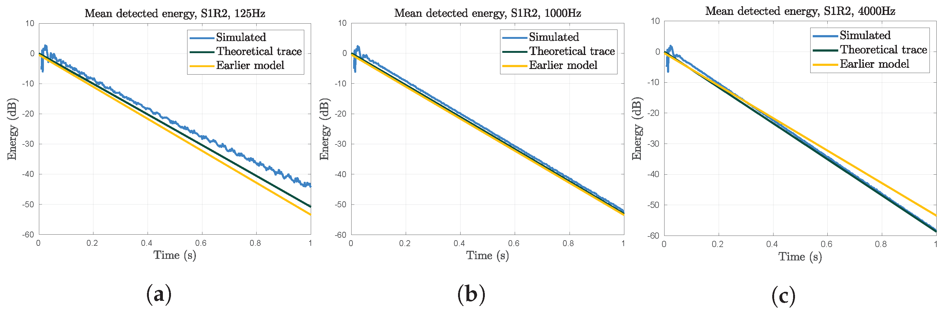
In Figure 3, the expected value estimated both from simulations and theoretical expressions is compared. As expected, the theoretical expressions are less accurate when the sound field is less diffused, in the early parts of the impulse response and in cases with low scattering. In these cases, the theoretical estimates tend to underestimate the total detected power. Since diffused sound fields generally tend to decay faster and have lower energy overall, this supports the theory that the simulated sound field is not diffused in these cases.

The two theoretical expressions are very similar, especially when air attenuation has no significant impact. When air attenuation affects the results, the newly derived estimate is significantly better. This is not surprising, and it is worth mentioning that air absorption can very easily be added also to the older estimate. When air absorption is not significant, the new estimate of the expected value is slightly smaller, as compared to the previous estimate. Since the earlier estimate makes an even stricter assumption on the diffuseness of the sound field (as discussed in Section 3.1), this can be interpreted as the earlier expression describing a more diffused sound field, which consequently has lower energy.

In Figure 3a, the expected detected energy for the octave band centered on 125 Hz is shown. In the results from simulations, a ringing behavior is seen. This is likely due to rays following a cyclical path through the simulated space, hitting the detector once every lap. Since all rays are emitted at the same time, $t=0$, all rays following the same path hit the detector at the same time. This behavior can be seen in ray tracers if the simulated space have very low scattering. It is not related to acoustic resonance.

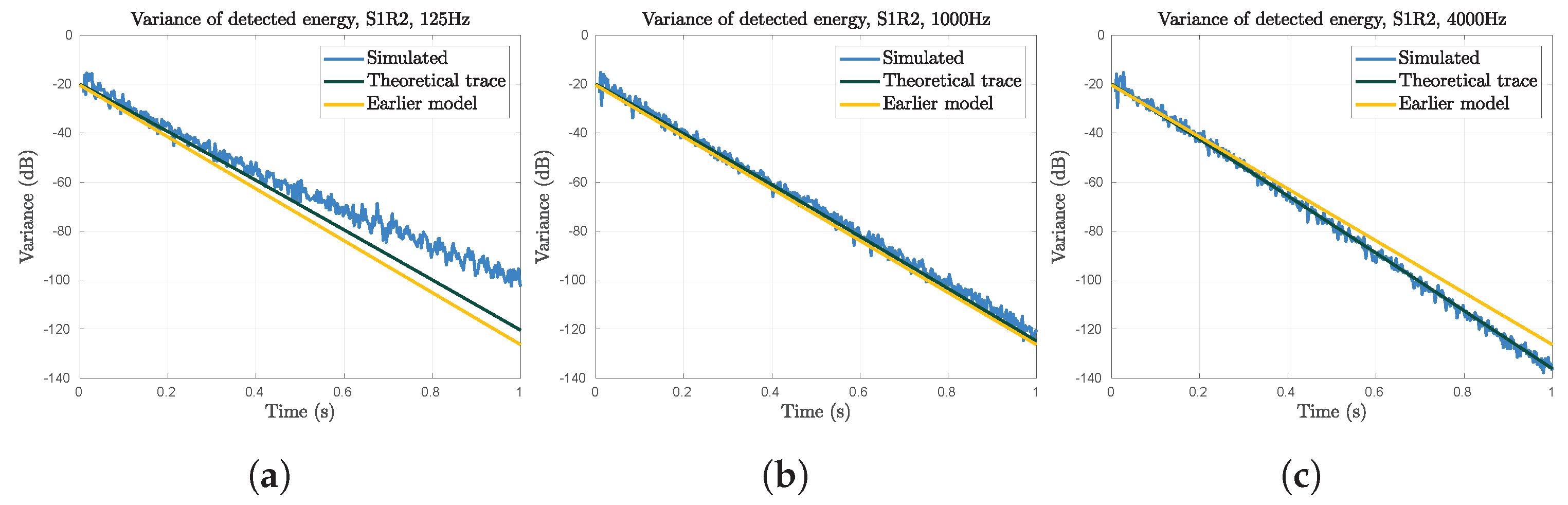
In Figure 4, the theoretical estimates of the variance are shown, together with an estimate from 15 simulations. Although the variance estimate derived from simulations is more noisy, its general trend (when the sound field is sufficiently diffuse) is matched very well by the theoretical expressions. The influence of simulation noise on the estimate of the variance is expected to be larger than its influence on the expected value, since the variance is approximately squared, compared to the measurement data itself. This amplifies all noise.

The results found for the expected value are mostly replicated in the results for the variance. That is, the theoretical expressions are more accurate for higher scattering and not accurate for the very early impulse response. In addition, it is found that the simplified expression and the expression derived in this paper are similar. When air attenuation affects the simulation, the expression which takes this into account is significantly better.

In Figure 5, the expected energy for each time is shown for increasing number of rays. Both the theoretical expressions are independent of the number of rays and are shown as horizontal lines in the plots. The estimated results do not show any dependence on the number of rays. As noted in Section 1, the expected value of Monte Carlo simulations should be independent of the number of samples, and any result other than what was found here would be alarming.

In the three graphs in Figure 5, the simulation results are slightly larger than the theoretical estimates (as was found in Figure 3), possibly due to the level of diffuseness in the simulations not reaching the level of diffuseness assumed in the theoretical expressions. However, the difference between the simulated result and the theoretically calculated results does not seem to change as time grows from 0.15 s to 1 s. A possible explanation is that the sound field after 0.15 s has reached its maximum level of diffuseness.

The variance, as it depends on the number of rays, is shown in Figure 6. As noted in Section 3.1, the variance decreases as the number of rays increase. The rate of change seems similar for all three graphs shown, but the computation noise in the simulated data is too large to make more precise statements.

5.2. Validation of the Algorithm

In this section, the results from the classical and the iterative algorithms are compared. In particular, it is examined whether the precision and accuracy of the two algorithms are equivalent for a large number of rays. This is primarily evaluated by comparing the estimated expected value and variance of the impulse responses produced using the maximum number of rays. Some room acoustic parameters are also studied to help determine whether the two algorithms produce perceptually similar responses. The room acoustic parameters are shown, together with measurement data for the space in question, to put the results into context. For a more detailed discussion of the correspondence between measurements and simulations, the reader is referred to [15].

As an initial test, the total detected energy in the broadband impulse response (simply the sum of all the energy detected in each simulation) was compared using a Mann–Whitney U test (Wilcoxon rank sum test) [23,24]. This is a non-parametric test on two data sets that indicates the likelihood that these or more dissimilar measurements could come from identical populations. As such, low values on the test signifies a higher likelihood that there is a difference between the two data sets. In this case, no significant difference could be found between the classical and the iterative algorithms. The results are shown in

Table 2. p-Value from a Mann–Whitney U test comparing the total energy detected in the impulse response for the iterative and classical algorithms. The results do not show a significant difference between the two data sets for any of the positions.

	S1R1	S1R2	S1R3	S1R4	S2R1	S2R2	S2R3	S2R4
p-Value	0.23	1.00	0.74	0.15	0.13	0.71	0.19	0.37

for each source and listener position separately, since the impulse responses for each source and listener position are unique.

The mean detected energy in the broadband impulse response was compared for the two algorithms, and some sample graphs are shown in Figure 7. The full set of graphs are available in the supplementary material. No significant differences can be seen. In particular, the results for the very early parts, containing the vital early reflections, are almost identical. Towards the end of the response, some discrepancies can be seen, but these are small in absolute terms and likely due to simulation noise. The similarities in the early response and in the decay rate show that the estimated expected values are very similar and likely at least perceptually identical.

In addition to comparing the mean of the simulations, the estimated variance was compared, as shown in Figure 8 and in the supplementary material. The estimates of the variances are more noisy, similarly to the variance found when checking accuracy of the theoretical estimates. It seems that the variances of the two algorithms have an equal decay rate over the impulse response.

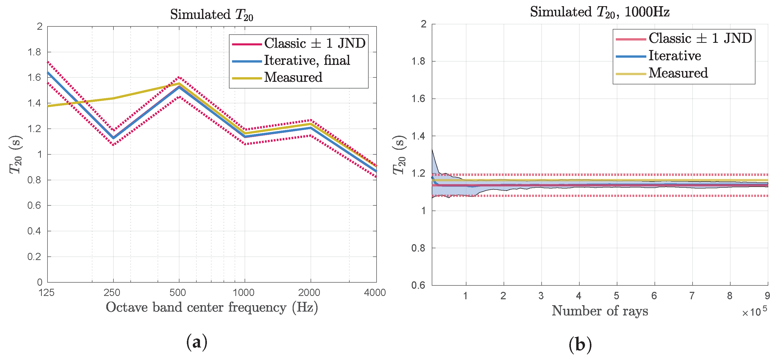
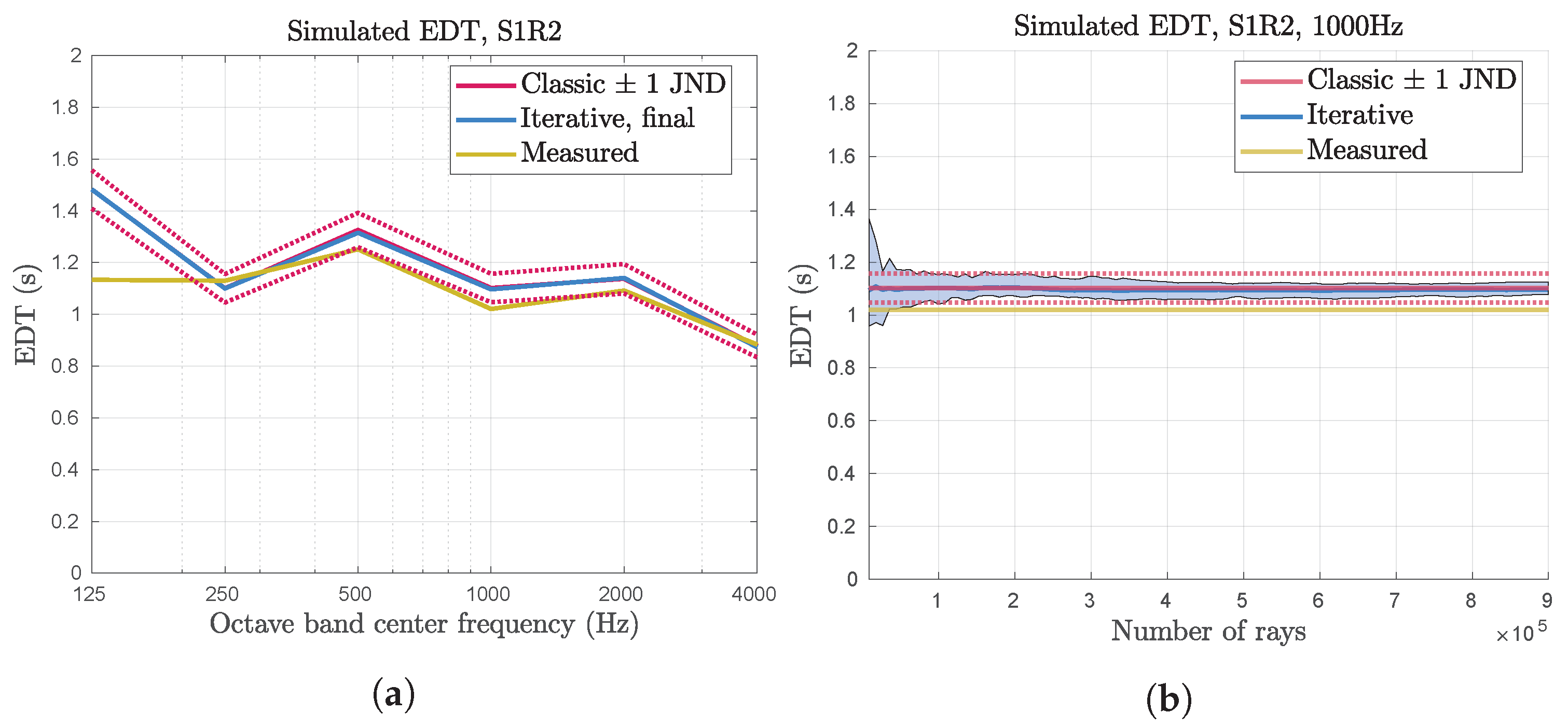
In addition to comparison of the broadband energetic impulse response, the reverberation time $T_{20}$, early decay time (EDT), and speech clarity $C_{50}$ were studied. Some results are shown in Figure 9a, Figure 10a and Figure 11a. In these graphs, the averages from 15 simulation runs are shown for the maximum number of rays. The reverberation time $T_{20}$ has been spatially averaged, in accordance with [20]. No significant difference can be seen between the estimated expected value of the two algorithms for any of the room acoustic parameters.

For the iterative algorithm, the room acoustic parameters were also studied, as the number of steps and, consequently, the number of rays increased, as shown in Figure 9b, Figure 10b and Figure 11b. Based on the calculations in Section 3.1, the expected value of the impulse response should be constant while the variance decreases. This should translate to a decrease in variance of the room acoustic parameters as the number of steps increase, but it does not necessarily mean that their expected value is constant.

In the graphs shown in Figure 9b, Figure 10b and Figure 11b, the room acoustic parameters for the octave band centered on 1000 Hz are shown as the number of steps in the iterative algorithm increases. The average from 15 simulations is shown as thick lines, and the area between the minimum and maximum parameter values is shaded. This illustrates the spread of the estimates over the whole set of simulation runs. As expected, the variations decreases as the number of steps increase, and when the total number of rays reaches about 100,000 (about 11 steps), the variations are about 1 JND.

It can also be noted that the estimated expected values for reverberation time $T_{20}$ and $C_{50}$ are not constant for all steps in the iterative algorithm. It is possible that this reflects a real effect for small numbers of rays, where the increased variability in the impulse response leads to a systematic difference in the calculated room acoustic parameters. It is also possible that the increased variability leads to a situation where the sample size of 15 is not large enough to ensure that the expected value is estimated accurately. However, the estimated expected values does not look particularly noisy, even for small numbers of steps, so it seems more likely that there is a systematic difference, due to how the room acoustic parameters are calculated.

As discussed in Section 4, the room acoustic parameters were used as a tool to estimate an appropriate number of rays to use in the iterative algorithm. The chosen number of rays is 81,000, and it can be seen in Figure 9, Figure 10 and Figure 11 that, for this number of rays, the variations of the room acoustic parameters are about 1 JND for this frequency band.

5.3. Computation Time

Iterative ray tracing is expected to improve the performance of classical ray tracing by adapting to the speed or precision as necessary. The results presented so far focus on showing that the iterative algorithm is as precise as the classical ray tracing algorithm, given sufficient time. In this section, the performance, in terms of speed, is evaluated. One aspect that is considered is how the time consumption per ray changes when iterative ray tracing is implemented. Another aspect is how large the overall time improvement is when the number of rays is decreased, as this indicates if it is possible, in general, to come closer to real-time performance by using fewer rays. As mentioned in Section 4, the ray tracer used in this study is not fully optimized for speed and cannot achieve real-time performance. The number of rays to use in each step of the iterative algorithm was consequently determined using other parameters and set to 81,000. For the classical ray tracing step, the full number of rays used was 540,000. Based on earlier research, this is sufficient for the space in question [15].

The simulation time for each algorithm is shown in

Table 3. Comparison of the time consumption for the classical algorithm and for the iterative algorithm. Computation time is presented for the ray tracing simulations and the transfer of simulation results from the graphics card to the host computer.

Algorithm	Ray Tracing Average ± std (s)	Transfer Average ± std (s)
Classic, 540,000 rays	$2.055\pm 0.039$	$0.0250\pm 0.0012$
Iterative, 81,000 rays	$0.307\pm 0.003$	$0.0260\pm 0.0004$

. The ray tracing average is the average time for a full ray tracing step, yielding energetic impulse responses for six octave bands and four listener positions. The retrieval average details the time consumption for transferring the impulse response data from the graphics card to the host computer (consisting of twelve impulse responses 8 seconds in length with a sample rate of 44.1 kHz). The update trace takes about 15% of the time required by the full simulation. The number of rays used in the iterative algorithm is also 15% of the number of rays used in the full simulation, which suggests that the time consumption is proportional to the number of rays, at least in this implementation of ray tracing. It is also noted that the data retrieval step takes longer for the iterative algorithm. This is due to the additional step of adding the calculated impulse response to that which has been calculated in previous time steps. The increase in total time is short, however.

The iterative algorithm reaches and exceeds the number of rays in the classical algorithm after seven steps with the current configuration. Assuming that the total time of a simulation is adequately estimated as the sum of the two steps detailed above, seven runs would take approximately 2.33 s, or about 0.3 s more than a full classical trace. The total number of rays in the classical trace is then exceeded by 27,000 rays. In total, the time consumption per ray is approximately 7% higher in the iterative algorithm in this specific configuration, and the approximate time consumption per ray is 4 μs for both algorithms.

6. Discussion

In this paper, an algorithm that improves the adaptability of ray tracing simulations in real-time applications has been presented. When the simulation time limits imposed by real-time performance negatively affects the simulation precision, iterative ray tracing can be used to improve simulation precision over time, eventually reaching optimal ray tracing performance. It is shown that the simulations produced by the iterative algorithm are equivalent to those produced using the classical algorithm with the same total number of rays, by both revising the theoretical estimates of the expected value and variance and comparing results from the two algorithms outright.

Additionally, a theoretical expression is derived for the expected outcome and variance of a ray tracing simulation in a diffused sound field. These expressions can be used to increase understanding of ray tracing simulations and their variability, which can help in determining what number of rays to use and what factors affect the reliability of ray tracing simulations. In addition, since ray tracing simulations are an unbiased tool for calculating the energetic impulse response predicted by a geometrical acoustics model, the estimated expected value can be used explicitly to find the impulse response of a space. This is only accurate if the sound field is diffused, and in real spaces, the sound field is practically never diffused. However, the later parts of the sound field, in some cases, can be approximately diffused. The expression could, thus, be an acceptable way to estimate the so-called reverberating tail of the impulse response.

The calculated expected value and variance are very similar to previously derived estimates, while being rather more complex to evaluate. The increased complexity is introduced as both the ray paths and the ray energy are considered stochastic, and the expressions in this paper can, consequently, be said to be more stringent, at least in that aspect. In that sense, the presented calculations show that the simplifications made in earlier derivations are appropriate at least in some spaces. The results presented in this paper also emphasizes that air absorption should be considered.

The iterative ray tracing algorithm has a similar performance as the classical algorithm if the total number of rays is equal. This is shown using the theoretical expressions for expected value and variance by examining the room acoustic parameters and by outright comparing the average impulse responses from the two algorithms.

In general, the time consumption per ray is greater for the iterative algorithm. However, the difference is small. It is not likely that this effect, even in real-time applications, would be sufficiently large to have a significant impact on how many rays can be used in each simulation step.

Iterative ray tracing needs to be tested further before it can be deployed in real applications. Importantly, it is not yet clear whether the algorithm can be used to speed up the simulation without perceptual degradation. This needs to be tested by listening tests with users, preferably in full virtual reality. Furthermore, the resolution for the spatial discretization needs to be determined, although this can likely be estimated quite well from the existing research on acoustic virtual reality.

The future development of the algorithm could be focused on the spatial aspects. For example, linear interpolation is mathematically equivalent to the operations performed when combining the impulse responses from different runs. If the impulse responses are from different locations, the summation and normalization step gives a spatial interpolation of the various positions, and modifications of the normalization value can be used to change the relative position of the interpolated impulse response. This could be used to modify the spatial resolution and to counteract any issues introduced by it. It may also be possible to remove the need for an explicit spatial resolution by, instead, using a moving average process, where the current impulse response consists of a linear combination of several of the latest calculations. This would implicitly perform a spatial interpolation and potentially also mitigate the risks of perceptual degradation when a new impulse response is to be calculated.

An advantage to iterative ray tracing is that it can be used well in combination with other methods of improving ray tracer performance, in terms of either accuracy or speed. The algorithm requires that the results from different runs of the ray tracer are statistically independent, but it does not have any specific limitations on how the ray paths are calculated and is very flexible, in terms of what algorithms and models it can be combined with.

7. Conclusions

Iterative ray tracing improves the overall precision of ray tracing simulations when real-time restrictions may otherwise adversely affect simulation performance. In comparison to classic ray tracing, it is as fast, but can also iteratively improve the simulated impulse response over time. The algorithm is flexible enough to be used in conjunction with other methods of improving ray tracer performance, both in terms of speed and in terms of accuracy.

In this study, and for this test space, it was shown that using as few as 15% of the rays produced simulation results was accurate to within 1 JND of the studied room acoustic parameters ($T_{20}$, EDT, and $C_{50}$) approximately 75% of the time. This is seven times faster than what is needed for full accuracy. It has also been shown that iterative ray tracing can take advantage of this significant improvement in speed, while still providing full accuracy as quickly as the classical algorithm.

The next step in the development of the iterative ray tracing algorithm should be to determine an adequate spatial resolution and then implementing the iterative algorithm, in conjunction with a fast ray tracing step and a real-time auralization engine.