Prediction of Head Related Transfer Functions Using Machine Learning Approaches

Abstract

The generation of a virtual, personal, auditory space to obtain a high-quality sound experience when using headphones is of great significance. Normally this experience is improved using personalized head-related transfer functions (HRTFs) that depend on a large degree of personal anthropometric information on pinnae. Most of the studies focus their personal auditory optimization analysis on the study of amplitude versus frequency on HRTFs, mainly in the search for significant elevation cues of frequency maps. Therefore, knowing the HRTFs of each individual is of considerable help to improve sound quality. The following work proposes a methodology to model HRTFs according to the individual structure of pinnae using multilayer perceptron and linear regression techniques. It is proposed to generate several models that allow knowing HRTFs amplitude for each frequency based on the personal anthropometric data on pinnae, the azimuth angle, and the elevation of the sound source, thus predicting frequency magnitudes. Experiments show that the prediction of new personal HRTF generates low errors, thus this model can be applied to new heads with different pinnae characteristics with high confidence. Improving the results obtained with the standard KEMAR pinna, usually used in cases where there is a lack of information.

1. Introduction

The head-related transfer function (HRTF) is a personal function that describes the propagation of the sound from a source to the auditory system of a human subject [1]. This function is particular to each individual because it largely depends on the anatomical structure of each person and the location of the transmitting and receiving elements [2]. Thus, the use of generic HRTFs, which have not been adapted to each particular individual, has been demonstrated to inhibit a high quality sound experience, and, in many cases, generate disorientation and confusion [3]. This has led to a multitude of studies regarding the generation of near-field HRTFs based on the binaural sound measurement in the free field [4,5,6,7,8].

The head-related impulse response (HRIR) in the time domain or HRTF in the frequency domain is defined by some authors such as Blauert [2] as an acoustic filter from a sound source to the entrance of the ear canal. These functions define the relation between the location of the source, the particular form of the listener’s auditory system, and the final effect on the sound. For this reason, each individual’s HRIR must be measured in order to improve the individual’s sound experience. The acoustic waves received by each individual are reflected and refracted by the pinnae, generating notches and peaks in the acoustic spectrum. Due to the variation of individuals’ pinnae, the HRIR and HRTF are unique to each individual [9,10,11,12].

Previous works to characterize individual HRTFs have been mainly categorized into two different approaches [13]. The first is the most precise method to obtain individual HRTFs. Acoustic signals are measured in an anechoic chamber by placing microphones in the ear canals to perform the necessary measurements to characterize each individual [14,15]. The second approach is less precise but it is faster and uses fewer resources. Acoustic signals are generated by predictive models, obtaining a good approximation of the characteristics of each user [16,17,18].

The problem is that obtaining these functions for each individual requires the use of special equipment and the cost of working time of experts. Machine learning methods are a very useful tool to solve this problem, as they can generalize new information based on historical data that defines the problem. Several studies in this field have used machine learning techniques in relation to HRTFs [19,20,21,22,23,24,25,26], although they used different methodologies and had different objectives in comparison to the current study. These works demonstrated how these techniques can be used to optimize and customize HRTFs with accurate results [11,27,28,29].

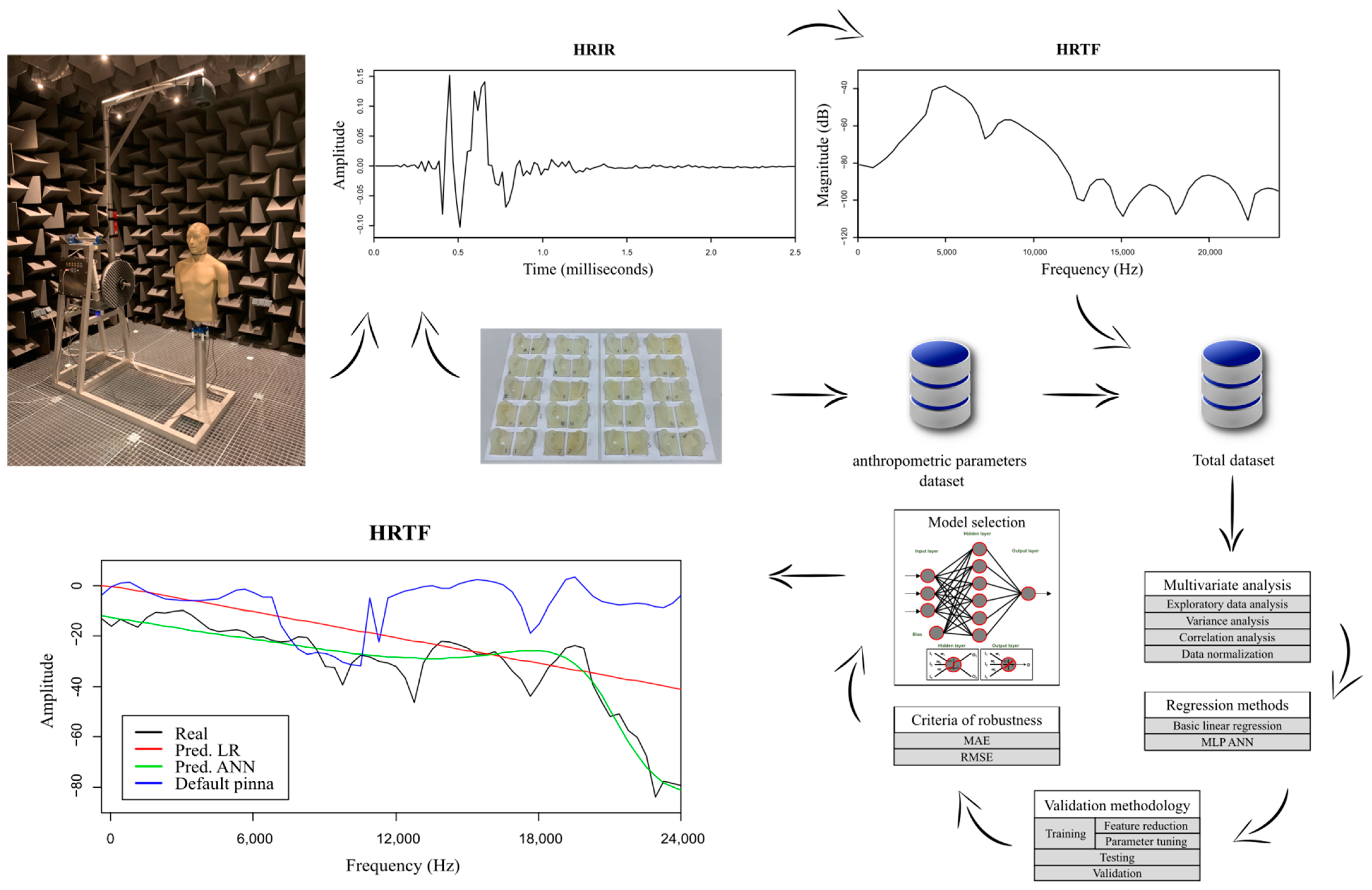
This work introduces a new approach to personalize HRTFs using machine learning techniques. The process is explained in the flow chart shown in Figure 1. Here, several models generalize the relation between HRTFs, source location, and individual ear shape. Two models were developed: a linear model, based on linear regression, and a nonlinear model, based on multilayer perceptron artificial neural network [30]. The applied prediction methodology was based on a training and testing process which optimized and generalized the model’s predictions while avoiding any possible overfitting. Initially, a multivariate analysis was performed to analyze the available dataset with two goals: build a more accurate model and have a better understanding of the problem. Later, a repeated cross-validation training was conducted. During this process, the most significant parameters of each algorithm were adjusted to improve the accuracy of the obtained models [31]. During this step, some robustness criteria were applied as help along the optimization of the training process, with the goal of selecting the most accurate models. Finally, the models with the best predictive behavior were selected and tested with information not previously used during the training. Obtaining in this way the real regression capacity of the model, preventing overfitting [32,33].

Finally, an analysis of the results was performed to know the reliability of the prediction and the efficiency of the applied models. Additionally, in this analysis, the obtained results were compared with the HRTFs measured using standard pinnae in order to verify if the models had a more accurate behavior than the standard HRTFs and thus could be used to improve the quality sound experience.

The remainder of this paper is as follows. Section 2 describes the Viking2 dataset which was used for the study and the new features under analyses. In addition, Section 2 describes the analyses that were performed, the results of which are presented in Section 3. Finally, Section 4 contains some concluding remarks.

2. Materials and Methods

This work was performed based on the Viking2 dataset [34], which contains both acoustic and anthropometric data for 20 individuals. Section 2.1 describes the acoustic measurements and Section 2.2 describes the anthropometric features used in this study.

Then, in Section 2.4, Section 2.5, Section 2.6, Section 2.7 and Section 2.8, the followed methodology is explained. How two techniques, one linear and one nonlinear, were applied to the problem under consideration, obtaining the prediction of HRTF based on personal anthropometric data of the pinnae and the position of the sound source. For this purpose, a multivariate analysis and a training/testing methodology were used, with the aim of developing a better understanding of the problem and predicting the amplitude of each frequency in the HRTF.

2.1. Acoustic Measurements

The acoustic data in the Viking2 dataset consists of a series of HRIR measurements for each of the individuals. Each HRIR signal is measured on a KEMAR mannequin equipped with a replica of the corresponding individual’s left pinna. The mannequin is mounted on a 360° rotating cylindrical stand and a Genelec 8020CPM-6 loudspeaker mounted on an L-shaped rotating arm. These signals were gathered at the University of Iceland in an anechoic environment with a focus on extra median plane measurements. The dataset includes full-sphere HRIRs measured on a dense spatial grid (1513 positions). These 1513 positions mark the location of the sound source, which is defined by the azimuth angle $\theta$ and elevation angle $\varphi$ in vertical-polar coordinates. Elevations are uniformly sampled in 5° steps from −45° to 90°. Azimuths are sampled based on

Table 1. Parameters that define the position of the source in each HRIR measurement.

Elevations [$°$]	[−45, 45]	[50, 70]	[75, 85]	90
Step [$°$]	5	15	45	360
No. of azimuths	72	24	8	1

in order to obtain a uniform density of the sphere. An overview of the methods and procedures of how HRIR signals were measured can be found in Spagnol et al. [4] and Onofrei et al. [35].

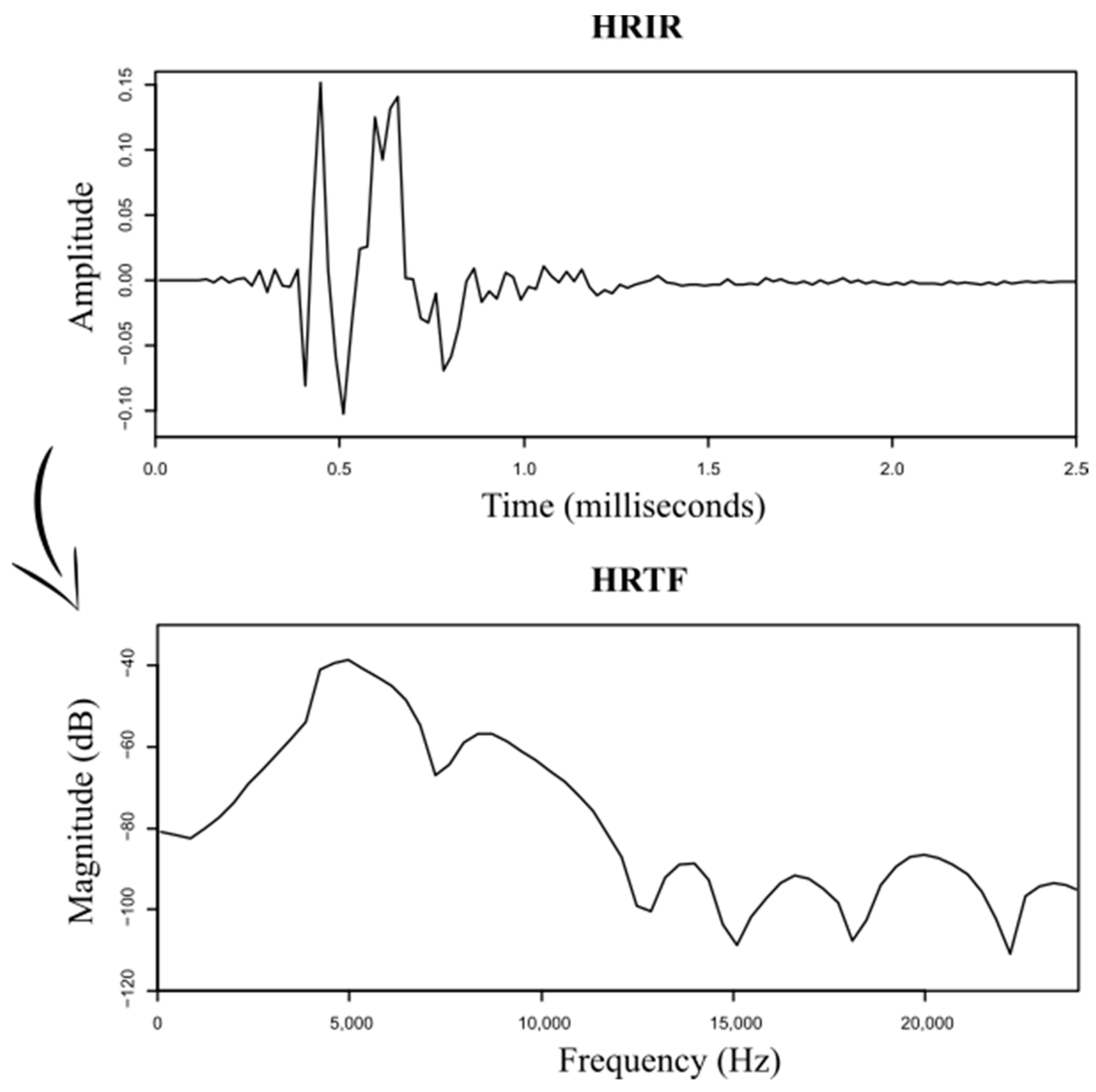
Starting from these measured HRIR signals, the corresponding HRTFs were obtained, from which the amplitude in dB was generated to be added to the final dataset. Sixty-five instances per ear type and per position were calculated, covering the frequency range from 0 to 24 kHz (Figure 2).

2.2. Anthropometric Data

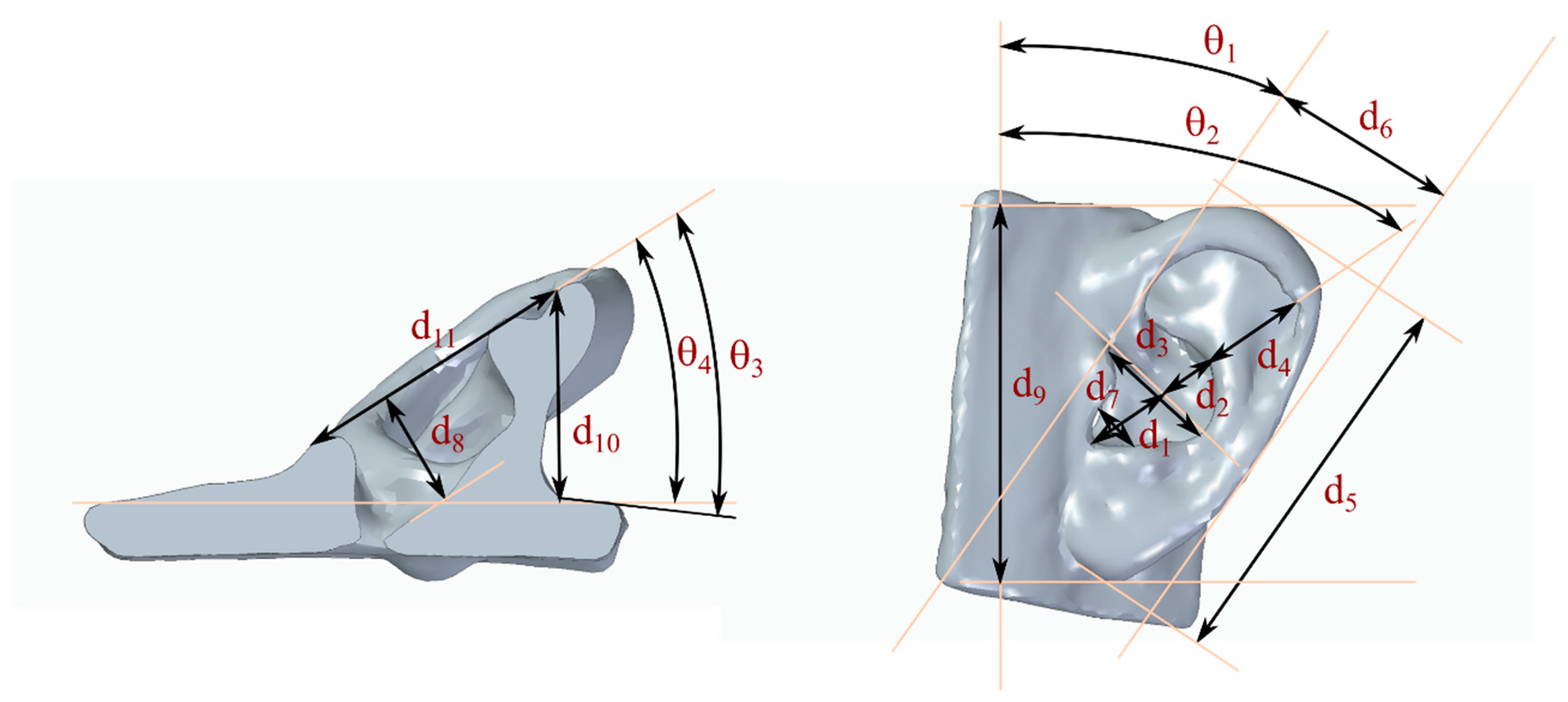
A second source of information, based on these same 20 artificial pinnae, was also used. Measurements of 15 pinna anthropometric parameters, including 11 linear and 4 angular parameters (

Table 2. Parameters measured in the pinnae.

Parameter	Definition	Units
$d_1$	Cavum conchae height	Millimeters
$d_2$	Cymba conchae height	Millimeters
$d_3$	Cavum conchae width	Millimeters
$d_4$	Fossa height	Millimeters
$d_5$	Pinna height	Millimeters
$d_6$	Pinna width	Millimeters
$d_7$	Intertragal incisures width	Millimeters
$d_8$	Cavum conchae depth	Millimeters
$d_9$	Physiognomic pinna length	Millimeters
$d_{10}$	Pinna flaring distance	Millimeters
$d_{11}$	Pinna posterior to tragus distance	Millimeters
${\theta }_1$	Pinna rotation angle	Euler degree
${\theta }_2$	Cavum conchae angle	Euler degree
${\theta }_3$	Pinna flare angle	Euler degree
${\theta }_4$	Pinna deflection angle	Euler degree

) were gathered for this work. There is currently no standard definition for these parameters; the parameters selected for this study are focused on obtaining a relatively integral representation of pinna features, following previous works found in the literature [8,36,37,38]. The anthropometric parameters of each pinna were measured from the 3D models used to manufacture silicone replicas of the pinnae (Figure 3).

Table 3. Statistics of the anthropometric parameters measured for this study.

	Mean	SD	Min	Max	Percentiles
					5th	10th	25th	50th	75th	90th	95th
$d_1$	18.71	3.06	10.96	22.96	14.34	15.11	17.47	18.78	20.33	22.69	22.88
$d_2$	8.83	2.43	5.36	14.53	5.76	6.08	7.42	8.33	9.72	12.44	12.97
$d_3$	18.59	3.37	13.43	25.91	13.83	14.07	16.31	18.09	19.95	23.12	23.90
$d_4$	20.87	4.90	11.23	30.39	13.40	14.96	17.74	21.17	24.09	26.20	28.51
$d_5$	68.03	6.15	54.66	81.95	60.90	61.53	64.28	68.23	70.40	73.42	79.18
$d_6$	33.75	3.88	27.20	41.84	28.94	29.11	30.78	34.09	36.70	37.17	40.11
$d_7$	7.25	1.38	5.32	10.19	5.52	5.70	6.03	7.07	8.00	9.23	9.32
$d_8$	11.27	1.95	7.65	15.00	7.97	8.73	10.38	110.24	12.47	13.76	14.18
$d_9$	66.64	6.03	53.16	79.33	58.65	58.98	63.74	67.28	69.07	71.88	77.94
$d_{10}$	20.07	3.81	14.14	26.92	15.72	15.88	17.22	19.21	22.10	25.83	26.29
$d_{11}$	27.92	5.33	17.98	37.06	20.61	20.79	24.32	28.93	30.58	34.96	35.22
${\theta }_1$	7.85	4.41	0.00	18.00	0.00	2.70	4.75	9.00	10.00	12.20	14.20
${\theta }_2$	25.95	6.64	14.00	42.00	15.90	19.60	21.75	25.50	30.00	32.50	37.25
${\theta }_3$	52.50	10.93	38.00	74.00	39.90	40.00	42.00	49.50	59.50	69.00	69.25
${\theta }_4$	38.70	9.93	24.00	59.00	24.95	25.00	31.00	40.00	43.00	49.60	55.20

summarizes the distribution of these anthropometric parameters, which indicates the parameter space covered by the final model.

2.3. Final Dataset

The final dataset was formed by a total of 21 features, of which 20 were independent variables that defined the only output variable, which was the amplitude of each of the frequencies that defined the HRTF. This study only considered the left pinna, and with this premise, the total number of instances that form the dataset was 1966900.

2.4. Multivariate Analysis

Initially, a general multivariate analysis was performed to obtain a better understanding of the problem and about the available data in order to make the most accurate prediction. For this purpose and to improve the precision of the built models, a study of the possible outliers, a correlation analysis, variance and covariance analysis, as well as a multivariate graphical analysis were performed [39].

2.5. Simple Linear Regression

The linear regression technique (LR) is applied to predict numerical variables using a model that statistically relates a dependent feature with several independent features through a linear relationship such as that shown in Equation (1).

$$y={\omega }_1{x}_1+{\omega }_2{x}_2+\cdots +{\omega }_n{x}_n+\epsilon$$

(1)

where $x_i$ are the independent features, $y$ is the dependent feature, ${\omega }_i$ are the weight coefficients of each independent feature obtained in based at the least squares method, $n$ is the number of features, and $\epsilon$ is the bias of this relationship.

2.6. Artificial Neural Networks

A multilayer perceptron artificial neural network (MLP ANN) is a feedforward single-hidden-layer neural network (given by Equation (2)); it has the ability to accurately predict complex nonlinear mappings inspired by the behavior of the biological neural system [40,41].

$$y={\displaystyle \sum }_{k=1}^s{\omega }_k{g}_k\left(b_k+{\displaystyle \sum }_{j=1}^n{x}_j{\beta }_j{}^{\left[k\right]}\right)+\epsilon$$

(2)

where $\epsilon ~N\left(0, {\sigma }_{\epsilon }^2\right)$, $s$ is the number of neurons, $n$ is the number of features, ${\omega }_k$ is the weight assigned to each neuron, $b_k$ is the bias assigned to each neuron, ${\beta }_j{}^{\left[k\right]}$ is the weight assigned to each variable that defines the network, and $g_k(·)$ express the activation function. In this case, the activation function is a sigmoid function for the hidden layer,$g_k\left(x\right)=\frac{1}{1+e^{-x}}$, and a linear function for the output layer. Finally, the method uses the Broyden-Fletcher-Goldfarb-Shanno (BFGS) algorithm to optimize the network and to find the internal weight constants, and also the decay parameter to avoid overfitting.

2.7. Validation Method

A validation process was necessary to analyze the precision with which the models define the problem. Several candidate models were built and trained based on different techniques and this evaluation must determine which one was the most accurate to solve the problem under study; the remaining models were discarded. In order to have the same weight for all the variables within the built models when making the prediction of the dependent variable, the first step in this process was to normalize the features that define the problem, in this case between 0 and 1. Subsequently, the dataset was divided into three blocks, the training dataset, the testing dataset, and the validation dataset.

The training dataset consisted of 17 pinnae (1,671,865 instances) and it was used to build and train the models. Two of the remaining three pinnae (196,690 instances) made up the testing dataset and were not otherwise used during training, with what they served to evaluate the real prediction capacity of the models. The last pinna was the standard KEMAR pinna (98,345 instances), which was used to validate the selected models. This validation was focused on analyzing how the predicted HRTFs improved the sound experience that can be obtained using the information of the standard pinna.

During the training stage, in order to avoid overtraining, a 50 repeated 10-fold cross-validation process was applied, where the parameters that defined the algorithms were tuned to optimize the precision of the models (

Table 4. Tuned parameters during the training stage for each of the regression techniques applied in the analysis: brief definition and applied range.

Regression Technique	Parameters	Range
LR	no tuning parameters	-
MLP ANN	size: number of units in the hidden layer	1–20
	decay: regularization parameter to avoid over-fitting	0–0.1

). The process was repeated several times, since the MLP ANN algorithm uses randomly initialized weights that define their structure and the accuracy assigned to the models can vary depending on the values selected in each initialization.

Finally, the most accurate models, when predicting the amplitude of each of the frequencies obtained for each technique, were selected from among the built models: one based on LR as a linear model, and one based on MLP ANN as a non-linear model. Using the selected two models, the behavior of how the prediction generalizes the problem was studied, along with the accuracy of the obtained results.

The whole process defined by this methodology was performed using an R statistical software environment v4.1.1 [42].

2.8. Robustness Criteria

To compare the different candidate models, an accuracy measure must be defined. In this work, the mean absolute error (MAE) and the root mean square error (RMSE) (Equations (3) and (4)) were used for this purpose, two of the most applied computational validation errors in supervised machine learning.

$$\mathrm{MAE}=\frac{1}{n}{\displaystyle \sum }_{k=1}^d\left|m_k-p_k\right|$$

(3)

$$\mathrm{RMSE}=\sqrt{\frac{1}{n}{\displaystyle \sum }_{k=1}^d{\left(m_k-p_k\right)}^2}$$

(4)

where $m$ are the measured values, $p$ are the predicted values, and $d$ is the number of instances applied into the validation process.

3. Results and Discussion

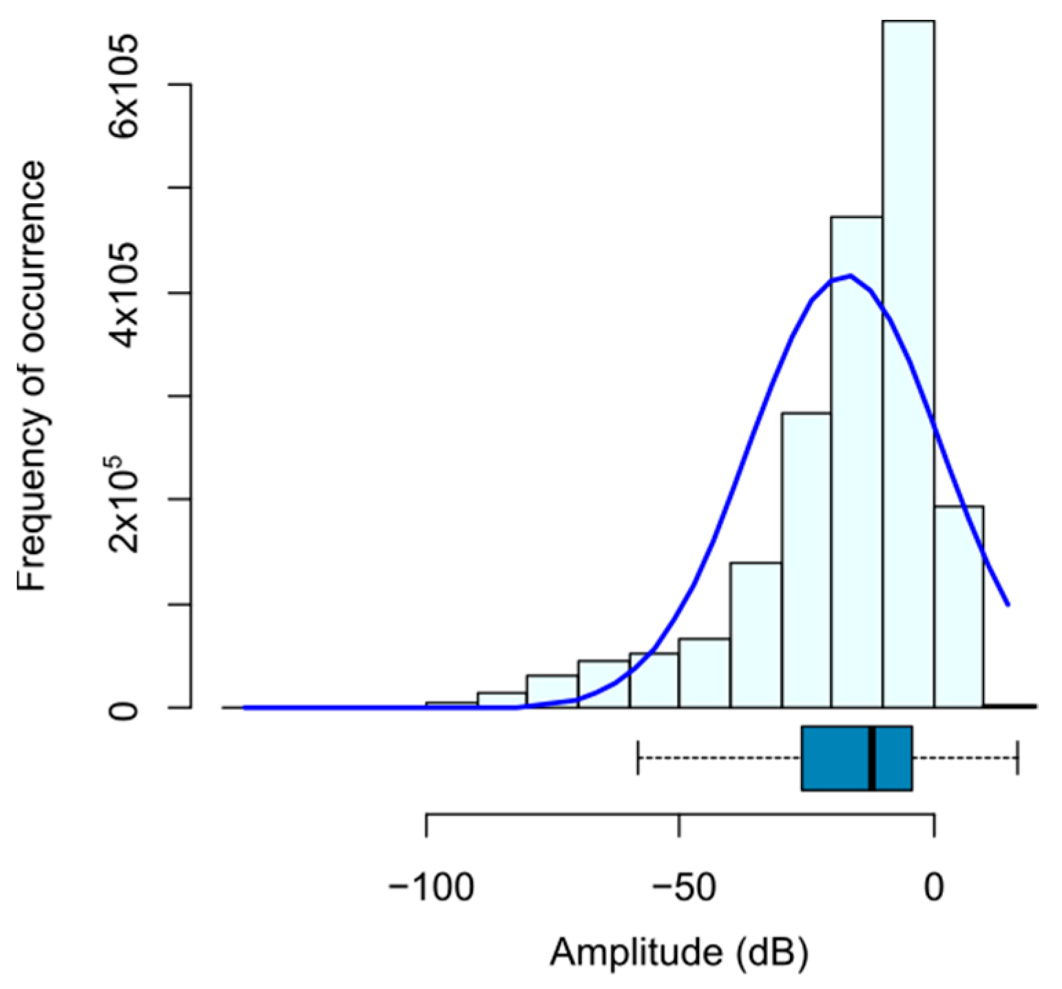
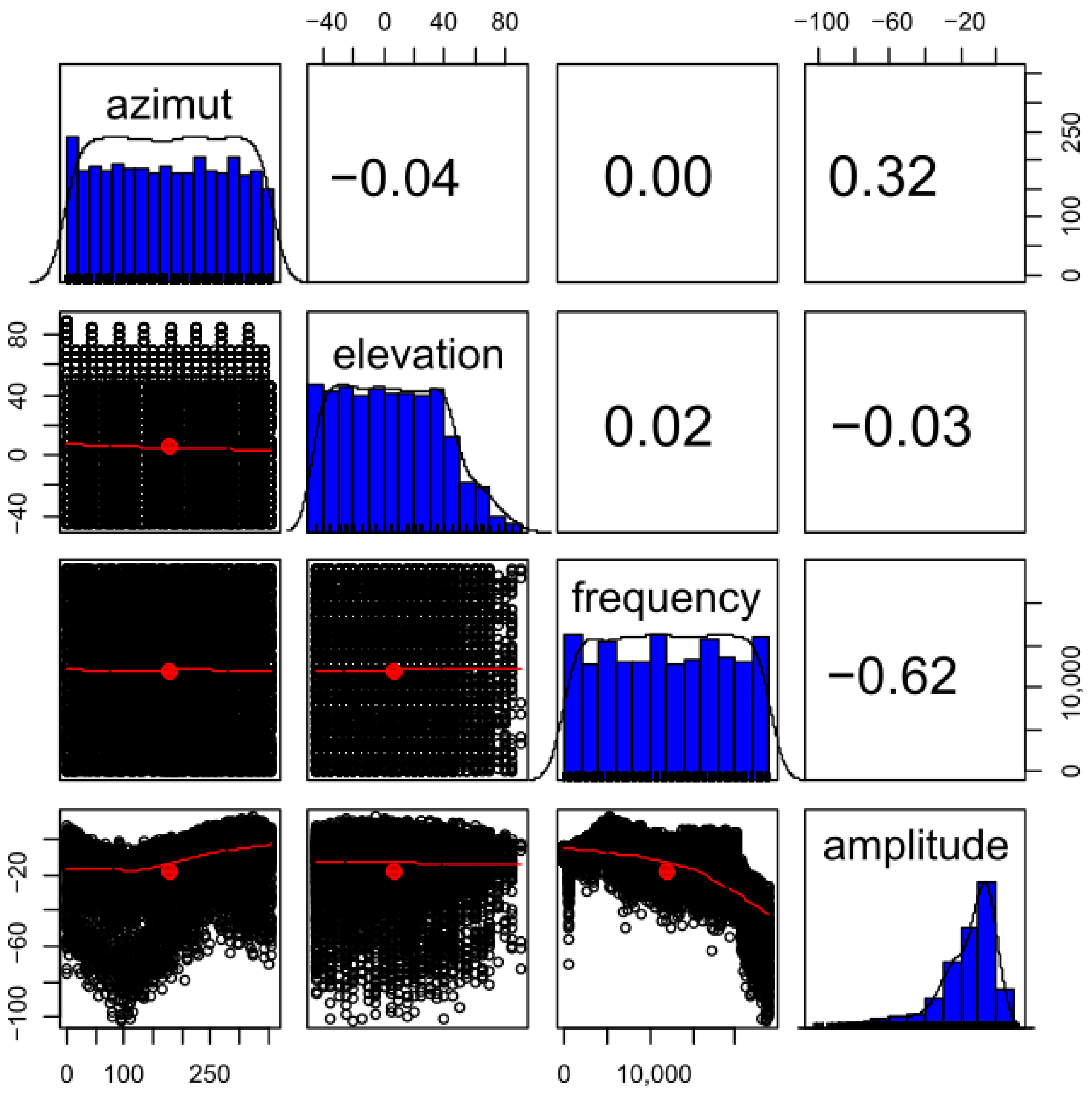
A multivariate analysis was performed to have a better understanding of the problem and to detect possible useless variables or instances in the final dataset for the problem under study. Within this analysis, the dependent variable was studied, and in this case it was the amplitude of each of the measured frequencies (Figure 4). It was found that the distribution was not completely Gaussian since it has a skewness of −1.56, and therefore the original dataset is slightly unbalanced. That means that the low amplitude values are more complex to predict.

Then, an analysis of variance (ANOVA) was performed to assess the uncertainty in the experimental measurements performed on the anechoic environment chamber. The amplitude of each of the studied frequencies were analyzed against the independent variables. The p-values obtained show low values for the most of the variables, indicating that the observed relationships are statistically significant (

Table 5. Results obtained from the ANOVA analysis for the predicted feature. Significant codes according to p-value: ‘***’ 0.001, ‘*’ 0.05, ‘ ’ 0.1.

	Estimate	Std. Error	t Value	p Value
Intercept	0.8738976	0.0012773	684.192	$<2\times {10}^{-16}$	***
$d_1$	−0.0114785	0.0013543	−8.476	$<2\times {10}^{-16}$	***
$d_2$	−0.0077947	0.0005956	−13.087	$<2\times {10}^{-16}$	***
$d_3$	−0.0084882	0.0007583	−11.193	$<2\times {10}^{-16}$	***
$d_4$	0.0190734	0.0009394	20.304	$<2\times {10}^{-16}$	***
$d_5$	−0.0045556	0.0055041	−0.828	0.4079
$d_6$	−0.0064500	0.0008496	−7.592	$3.15\times {10}^{-14}$	***
$d_7$	0.0082313	0.0006021	13.672	$<2\times {10}^{-16}$	***
$d_8$	0.0288839	0.0015689	18.411	$<2\times {10}^{-16}$	***
$d_9$	−0.0131845	0.0051347	−2.568	$0.0102$	*
$d_{10}$	−0.0168657	0.0005806	−29.050	$<2\times {10}^{-16}$	***
$d_{11}$	−0.0027780	0.0006965	−3.989	$<6.65\times {10}^{-5}$	***
${\theta }_1$	−0.0261202	0.0015868	−16.461	$<2\times {10}^{-16}$	***
${\theta }_2$	0.0062978	0.0010993	5.729	$<1.01\times {10}^{-8}$	***
${\theta }_3$	−0.0140979	0.0008816	−15.991	$<2\times {10}^{-16}$	***
${\theta }_4$	0.0142957	0.0007572	18.881	$<2\times {10}^{-16}$	***
azimut	0.1339585	0.0002315	578.635	$<2\times {10}^{-16}$	***
elevation	−0.0034120	0.0002842	−12.005	$<2\times {10}^{-16}$	***
frequency	−0.2717950	0.0002313	−1174.992	$<2\times {10}^{-16}$	***

). Thus, when the p-value is lower than 0.1, it is considered, with a low level of uncertainty, that the null hypothesis can be confidently rejected, and the independent variables give significant information to predict the independent variables. A low residual standard error of 0.08768 on 1671846 degrees of freedom is obtained. Finally, a correlation analysis was performed to identify and measure the relation among pairs of variables. For example, in Figure 5, the correlation found between the elevation angle, azimuth angle, frequency, and amplitude is shown. This correlation analysis confirmed what it could be observed with the analysis of variance, that the most influential variable for knowing the amplitude was the value of its frequency.

Once the multivariate analysis was completed and based on its results, it was observed that the independent variables adequately defined the dependent variable, and consequently with the available dataset it was possible to build and train accurate models based on the proposed methodology. However, attention should especially be focused on the residuals obtained by the models at low amplitude values, since the dataset was not totally balanced.

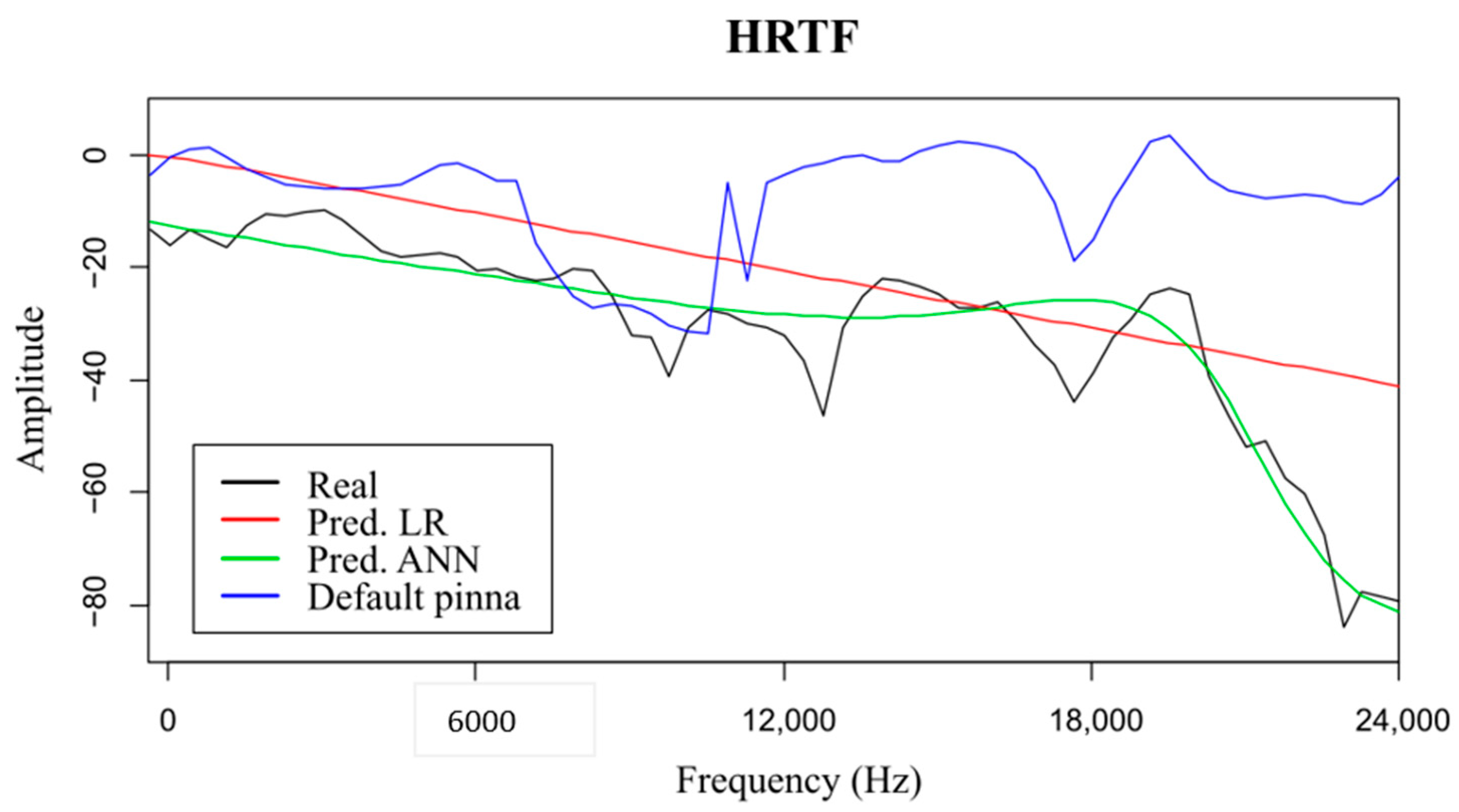
The first analyzed prediction method was a linear regression. The obtained results were promising since the calculated errors were low (

Table 6. Obtained results during the training and testing stage for the total dataset.

	Training		Testing
	MAE (%)	RMSE (%)	MAE (%)	RMSE (%)
LR	6.52	8.76	5.82	7.57
MLP ANN	2.66	3.66	3.54	4.58

and

Table 7. Obtained results during the testing stage for the pinnae ‘R’ and ‘S’, pinnae that form the test dataset. Additionally, it is shown the error committed in the case of using the standard KEMAR pinnae (Pinna ‘T’) instead of the models.

	Pinna R		Pinna S
	MAE (%)	RMSE (%)	MAE (%)	RMSE (%)
LR	5.84	7.62	5.81	7.52
MLP ANN	4.11	5.28	2.98	3.88
Pinna T	15.35	20.66	15.33	20.02

) and the predictions fit quite well with the trends of the original curves (Figure 6). This linear method also allowed knowing the relationship between the independent variables and the dependent variable (Equation (5)), giving a clear idea of the influence of each variable in the prediction of the amplitude at each frequency.

$$\begin{gathered} Amplitude=0.873898-0.011479·d_1-0.007795·d_2-0.008488·d_3+0.019073 \\ ·d_4-0.004556·d_5-0.006450·d_6+0.008231·d_7+0.028884 \\ ·d_8-0.013185·d_9-0.016866·d_{10}-0.002778·d_{11}-0.026120 \\ ·{\theta }_1+0.006298·{\theta }_2-0.014098·{\theta }_3+0.014296·{\theta }_4+0.133958 \\ ·azimut-0.003412·elevation-0.271795·frequency \end{gathered}$$

(5)

Although with the use of the LR technique, it was also observed that the model predicts with greater error the amplitudes that have lower values, and especially when there were abrupt variations in amplitude values between nearby frequencies (Figure 6 and Figure 7). As can be seen in Figure 7, the study of the residuals obtained supported this conclusion, obtaining a minimum value of −103.13, in the 1Q of −6.35, a median value of 0.03, a 3Q equal to 8.39 and a maximum value of 42.76. In addition, based on this analysis and focused on the Q-Q plot, it was observed that the samples within the quantile that defined the lowest amplitude values did differ significantly from the line that compares the real distribution with the predicted distribution.

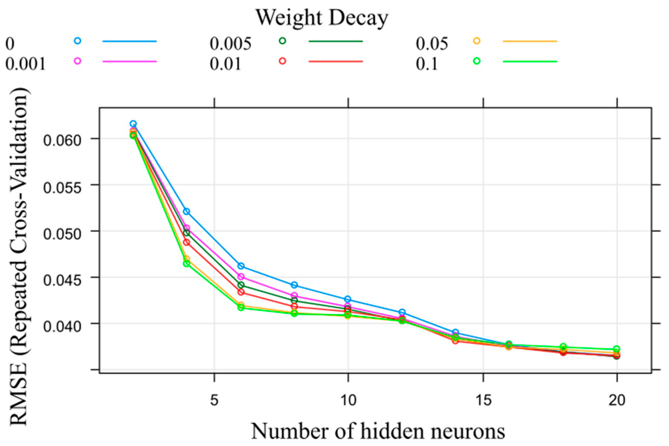
The study of LR results led to conduct another analysis using a non-linear model, in this case one model built based on MLP ANN. This new task was focused on improving the weaknesses of the linear model. To do this, during the training, a tuning of the most significant variables of the algorithm was performed at the same time as 50 times repeated cross validation (Figure 8). For this algorithm, it was concluded that the chosen neural network structure was formed by 20 neurons in its hidden layer and a weight decay value of 0.005, values that provided a model with accurate prediction results.

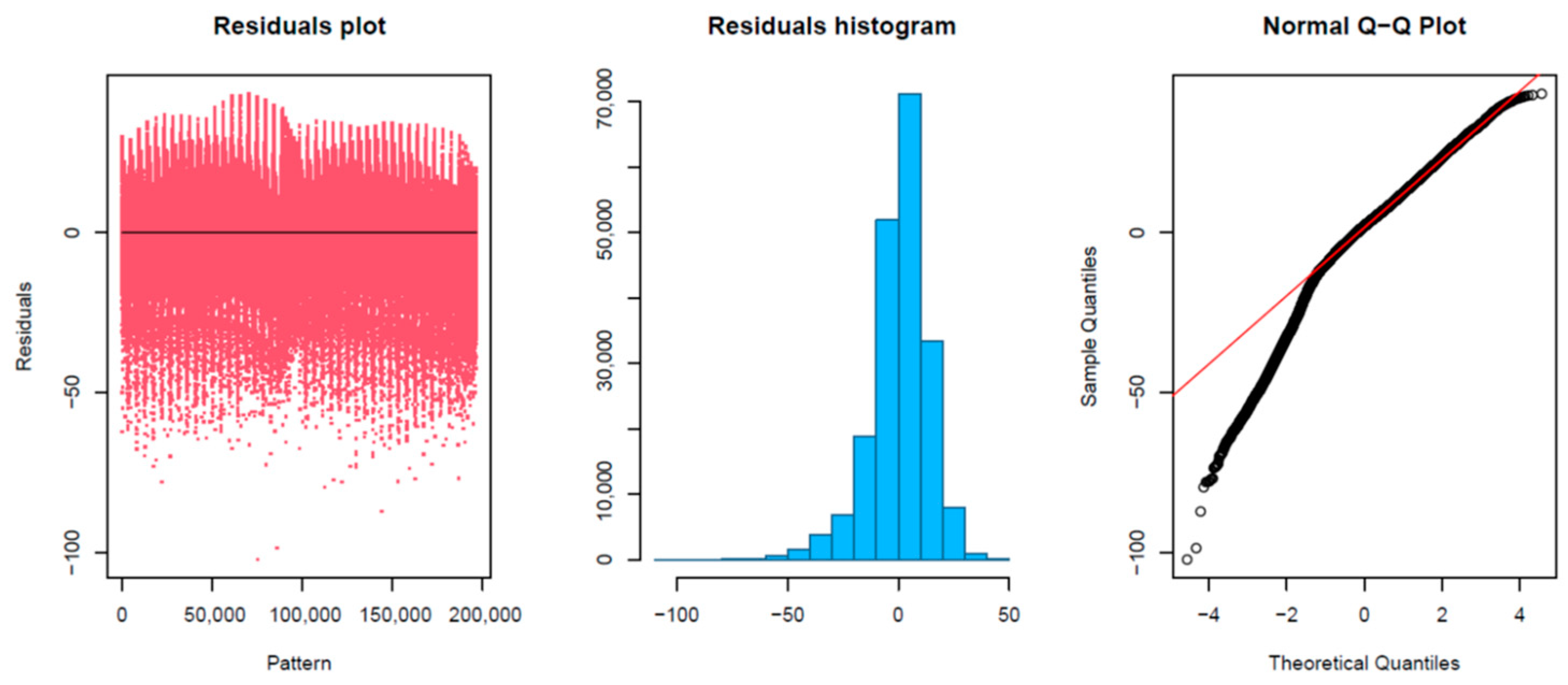
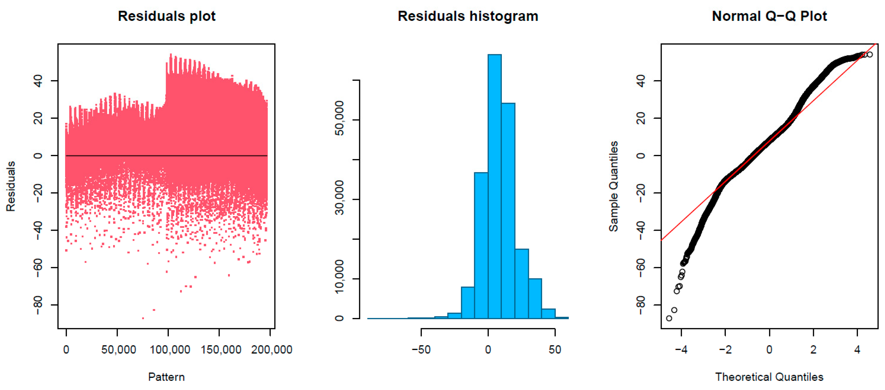
The use of this nonlinear model led to observe a more accurate prediction at low amplitudes and also, a better adjustment when there is an abrupt amplitude variation of nearby frequencies (Figure 6 and Figure 9). Additionally, in Figure 9, the study of the residuals obtained showed a minimum value of −87.05, in the 1Q of −8.23, a median value of 4.71, a 3Q equal to 12.83, and a maximum value of 54.14. In this last case, the residual plots showed a fairly random pattern with positive and negative residuals, indicating that the model provided accurate fit to the data. Furthermore, the residual histogram had a symmetric bell shape, and the normal probability plot followed the straight line in a more accurate way, mainly at the extremes of the graph where the linear model failed. It was also observed in Figure 9, a more marked difference in the residuals generated depending on each of the testing pinnae.

Finally, to check the methodology and the progress it provides in the field, the error obtained by the predictions was compared with the error that would be obtained in the case of using the HRTFs measured on the standard KEMAR pinna (Table 7). In this case, it was verified that both model predictions improved the results obtained with the standard pinna, but especially when the ANN-based model was applied. Although these models still did not very accurately predict possible frequency notches, they showed accurate results predicting the HRTFs trend and showed especially important improvements in comparison with the results obtained using the standard pinna. It can be concluded that these models supply useful information to obtain a higher quality sound experience, improving the information given by the standard pinna.

4. Conclusions

Based on the study performed on this work, two major problems have been observed when working with virtual personal auditory space. The first HRTFs that define the space change considerably with the morphological features of each individual. Additionally, the second HRTFs that perform all the measurements to obtain these functions for a new individual is a complex and expensive task. Faced with these problems, it has been observed that the use of multivariate analysis techniques can help considerably when studying how these functions vary, and also to understand their relationship with the morphological attributes of different individuals. It has also been proven that the use of supervised machine learning techniques applied to datasets adapted to the problem under study, allows predicting HRTFs with relatively low errors of new individuals with its personal morphological features, even if these differ from the individuals studied in the dataset used to train the models. It was also observed that to model a complex problem as HRTFs, linear techniques get greater errors despite generating important information related to the problem, for example an easy-to-understand-and-interpret mathematical equation that relates the features to each other. Furthermore, non-linear techniques better fit and generalize the problem in order to predict these functions. In addition, when the results obtained with these models and the results generated based on a standard pinna are compared, it is observed that the adjustment of HRTFs based on the morphological attributes of each individual is significantly improved. Application of more advanced algorithms in future enhancement could generate more accurate predictions and even detect frequency notches more clearly.