A Hybrid Multistep Procedure for the Vibroacoustic Simulation of Noise Emission from Wind Turbines

Abstract

This paper proposes an efficient hybrid analytical-computational approach for the simulation of mechanical vibrations and sound radiation in wind turbine drive trains.The computational procedure encompasses the detailed modeling of vibrational sources and structural sound paths as well as the major panels of airborne noise radiation. The angle-varying mesh stiffness is obtained from a series of quasi-static finite element simulations. A novel procedure is proposed to obtain the time-varying mesh stiffness at fluctuating speed. The varying mesh stiffness is introduced as a parametric excitation in an analytical gear model, and the Fourier-transformed results are used as vibrational sources in a finite-element-based harmonic response analysis of the drive train. The present paper focuses on the modeling of gear contact and gearbox vibrations. The models and procedures are outlined, and computational results are compared to physical measurements on a 2.5 MW wind turbine. The results are in good qualitative agreement at tonal frequencies. This is particularly the case at fluctuating speed, where both the simulation and the measurement show the characteristic effect of frequency modulation. The computational procedure has been expanded to the whole drive train and is effectively applied in the conception and evaluation of design measures for the reduction of tonal amplitudes.

1. Introduction

Noise emission from wind turbines is a critical issue that limits the social acceptance of the green technology [1,2,3,4,5,6,7,8,9,10]. Wind turbine manufacturers are particularly concerned with narrow band amplitude peaks called tonalities [11,12]. It is generally accepted that most tonalities in the radiated spectrum can be traced back to gear noise; i.e., parametric mechanical vibrations caused by gear interaction in rotating machinery [13]. The gear vibrations are transmitted via several structural sound paths to radiating structural panels, such as the gearbox walls or the nacelle. The tonal amplitudes can be ameliorated by technical design measures, either at the source, or on the transfer paths, or both. Sound is most effectively controlled at its sources but, in many practical cases, the sources are not accessible to design changes and noise reduction measures must be introduced along the sound paths. Computational simulation is the tool of choice for the vibroacoustic evaluation and optimization during the design stage. In order to predict the effects of design changes on the acoustic characteristics, the computational models should, on one hand, include the vibrational sources with sufficient accuracy but must, on the other hand, reach beyond the sources and include the major transfer paths. We demonstrate in this paper how these two goals can be achieved with an efficient hybrid analytical–computational multistep approach. We focus here on gear interaction and gearbox vibrations, but the computational efficiency of the procedure allows for further expansion onto the complete driveline, including the girder, the nacelle and other parts of wind turbines. Thereby, the present procedure significantly expands the scope of true-to-detail modeling in comparison with previous approaches. Furthermore, a novel procedure for calculating the frequency response at fluctuating operational speed is presented. It is demonstrated by comparison to physical experiments that the computed frequency response functions (FRF) are in good qualitative agreement with the measurements at major meshing frequencies. Comparing the results of test runs with fluctuating and constant speed, the well-known effect of “frequency smearing” [14,15] due to frequency modulation by fluctuating speed is observed, both in simulation and in measurement.

Gear vibrations are parametrically excited by the temporal variation of the contact configurations in gear pairings [16,17]. This effect of time-varying mesh stiffness [18,19,20] has been widely studied in the literature; see [21] and references therein. Chen [22] compares several meshing characteristics of helical gears, using both analytical and Finite Element (FE) methods. A number of other investigations, e.g., [23,24,25], compare numerical results from FE models with different analytical approaches. The computational models account for the flexibility of the components and represent in detail their geometric and material properties. They may, however, contain a large number of degrees-of-freedom (DOF), and transient simulations can be very costly. The accuracy of the FE results strongly depends on the modeling parameters, e.g., the element size, the contact tolerance or the selected element types [26]. In this context, Dai [27] emphasizes the inefficiency of pure FE models for the simulation of dynamic gear processes. Alternatively, Lumped Parameter (LP) models provide a computationally efficient option for dynamic simulation. Here, the components are included as rigid bodies, which are idealized as point masses and connected via discrete spring-damper elements. Such models contain significantly fewer DOF than FE models. A large variety of lumped parameter simulations for gear systems has been published [11,28,29,30,31,32,33,34]; see also the review papers [16,35,36,37,38]. The majority of these investigations deal with single-stage gear systems. Planetary or multi-stage gear systems are considered in [39,40,41,42,43,44,45]. The LP models do not, in most cases, include the gearbox housing and further components of the drive train. Luo [46] represents the gearbox housing by a set of lumped mass and stiffness parameters.

Many investigations are based on a combination of LP and FE modeling [40,43,47]. Hybrid computational models that encompass tooth contact, elastic foundations, bearings and pinions by combining finite element/contact-mechanics (FE/CM) with multibody dynamics formulations can be found in [27,48,49,50,51,52,53,54,55,56,57]. Most models and procedures in the literature focus on the gear-shaft-bearing connection. Only a few studies consider the vibrations of the entire gear-bearing-housing system [21,58]. Guo et al. [58] have developed a multistep computational procedure for determining the vibro-acoustic propagation of gear vibrations. The dynamic bearing forces and moments are calculated using either an LP or an FE/CM gearbox model. These forces are then applied as excitations in an FE model of the gearbox housing. The normal velocities on the surface elements are subsequently used for the acoustic simulation of the sound radiation with the boundary element method. Sound pressure results for unit bearing forces and moments are combined with separately computed bearing loads to determine the overall far field sound pressure. Zhou et al. [28] have presented a hybrid approach for the steady-state dynamic response of a single-stage gearbox. Using a series of static-structural FE simulations, the angle-dependent mesh stiffness is calculated and applied in a gear dynamic model with three degrees of freedom. The transient bearing forces from this model are applied as dynamic excitations in a structural FE model of the gearbox housing. The FE model is solved in the time domain to obtain the vibration response, which is subsequently used to calculate the acoustic radiation with a boundary element model. Helsen, Vanhollebeke et al. [10,59,60,61,62,63,64] have studied wind turbine drive trains with a flexible multibody technique. Their approach also includes vibroacoustic simulations for a wind turbine gearbox, where the bearing forces from the multibody model are applied to a flexible FE model of the gearbox housing. More recently, Xu et al. [47] have developed a dynamic FE/LP model for a helicopter gearbox that accounts for the flexibility of both the shafts and the housing. Based on this model, a time-domain method for identifying the resonance paths of a multistage gearbox was proposed. The entire model is simulated in the time domain in order to calculate the response to operating conditions, including varying speeds. Speed fluctuations are also considered by Sika et al. [65,66], who investigate the numerical stability of a gear contact model in the time domain.

In the computational approach presented herein, the frequency response for arbitrary measuring points, surfaces, and volumes of the gearbox and the drive train is obtained as the final result of an integrated multistep procedure. The computational chain starts from the calculation of the angle-varying mesh stiffness, using a series of static FE/CM analyses of all relevant gear pairings (spur and helical). Then, the time-varying mesh stiffness (TVMS) is computed from the angular variation of mesh stiffness. A novel technique is introduced here that accounts for temporal variations of the operating speed. Transient simulations with rigid-body models of gear pairings yield the dynamic transmission errors for the multi-stage gear system. The Fourier transforms of the transmission error are used as excitations for the harmonic FE analysis of the gearbox. The present FE model also includes the internal components (shafts, gears, etc.) of the gearbox, which are often neglected in related contributions [28,58,62]. Including the internal components not only increases the model accuracy, but allows also to apply the harmonic excitation precisely at the locations of gear contact. The gearbox mounts are represented in the FE model by six-dimensional stiffness and damping matrices.

In summary, our computational procedure significantly expands the range of true-to-detail modeling for the vibroacoustic simulation of wind turbines. The hybrid approach combines the transient analysis of the major sound source with the FE-based frequency response analysis of structural vibrations along the sound paths. A novel methodical feature accounts efficently but realistically for the influence of speed fluctuations on the frequency response. The vibroacoustic model is successfully validated by comparison to physical measurements. Sound radiation from vibrating panels can be readily evaluated by standard measures such as the equivalent radiated power, or by vibroacoustic structure-fluid coupling. A new effcient approach for the FE-based simulation of far-field acoustic radiation has been proposed by the authors in [67].

The remainder of this paper is organized as follows. The details of the hybrid computational procedure are outlined in Section 2. Section 3 describes the vibroacoustic simulation of a wind turbine gearbox and the comparison with physical measurements. We discuss the influence of varying operational speed and different load levels as well as the sensitivity of simulation results to the modeling of internal components. Detailed information is given about the computational cost and efficiency for the large-scale application. The main conclusions of the investigation are drawn in Section 4.

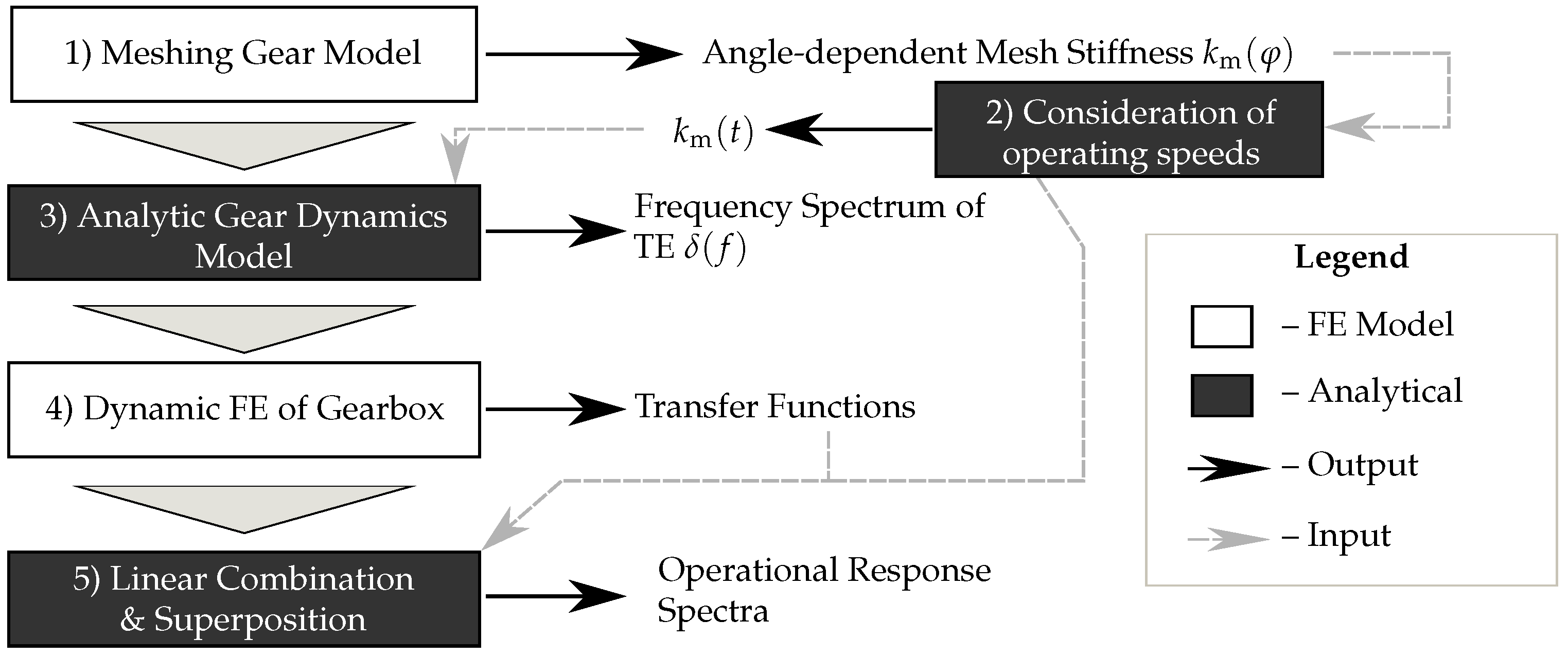
2. Hybrid Analytical-Computational Procedure

The proposed integrated computational procedure for the calculation of the operational response of wind turbine gearboxes consists of five sequential steps, shown in a schematic plot in Figure 1. In the first step, a series of static 3D FE simulations is performed to obtain the varying mesh stiffness at the gear contact for a number of meshing configurations over one mesh cycle. Using the results of the first step and the operating speeds of the gears, the time variation of the mesh stiffness is computed analytically in the second step. In the third step, the TVMS is used as an input for an analytical two-body model of a gear pairing which yields the transmission error (TE) $\delta$ at gear contact. The fourth step involves harmonic finite element analyses for constant TE amplitudes over the frequency range of interest for a detailed model of the gearbox and the drive train. The results are dynamic transfer functions from the gear contact to all points and measures of practical interest. The results of the third and fourth steps are combined in the fifth step to compute analytically the operational response of the gearbox and the drive train for arbitrary points, surfaces, and volumes of interest.

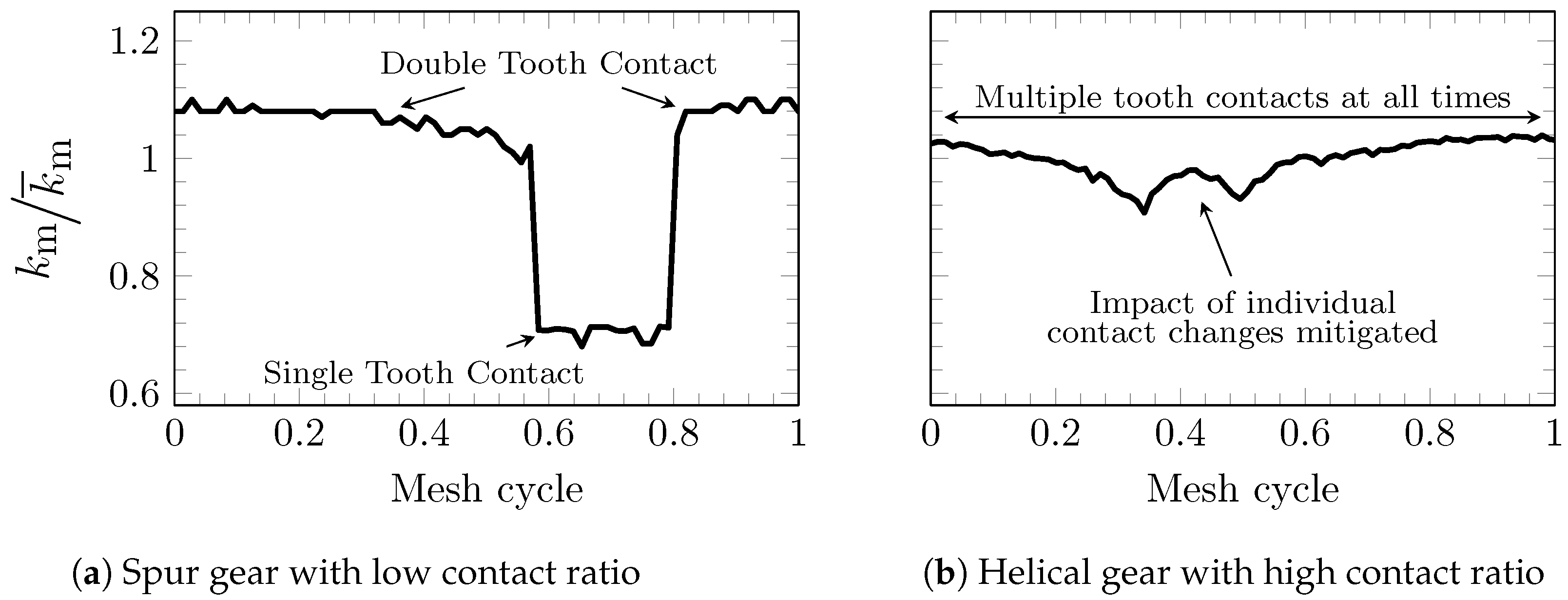
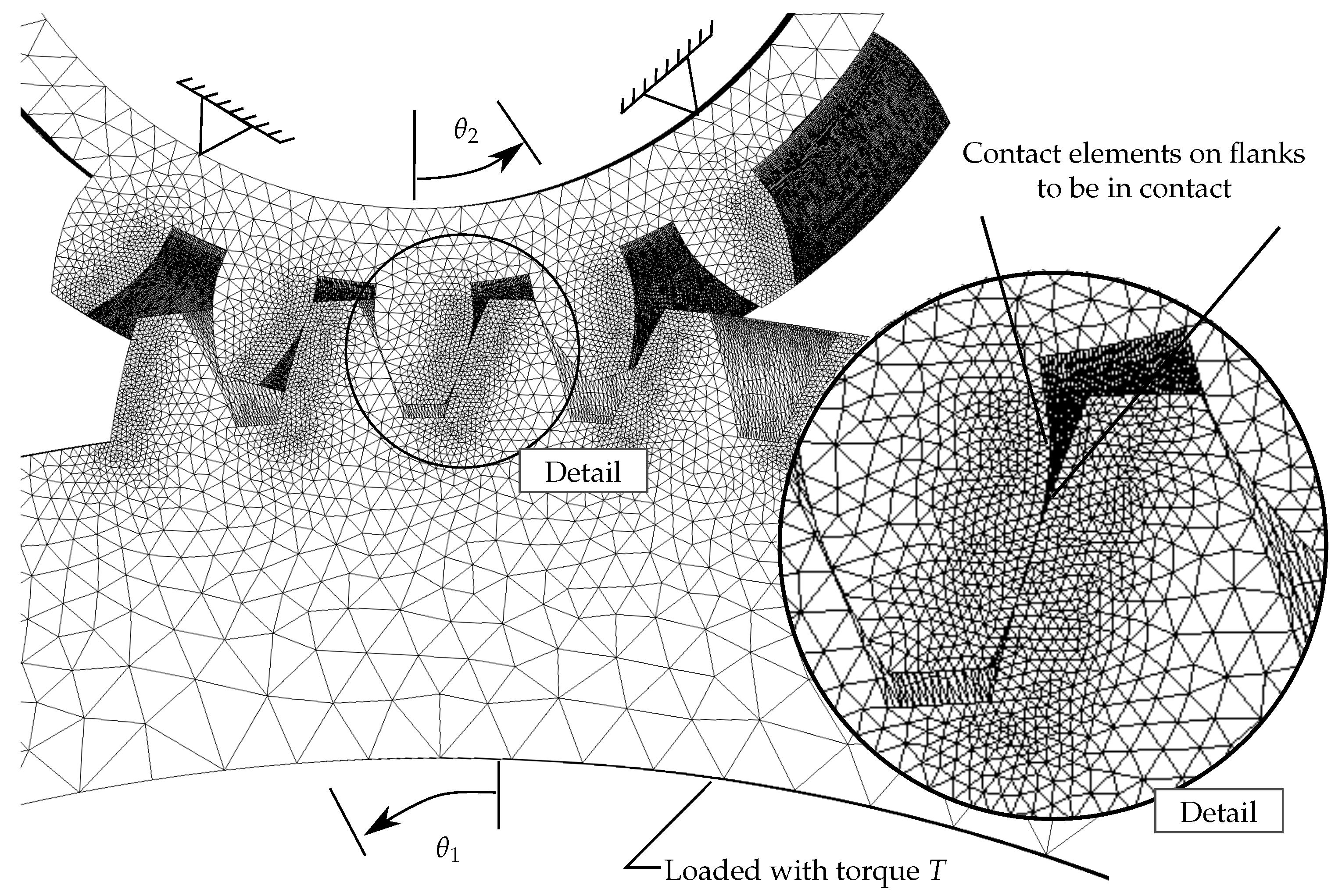
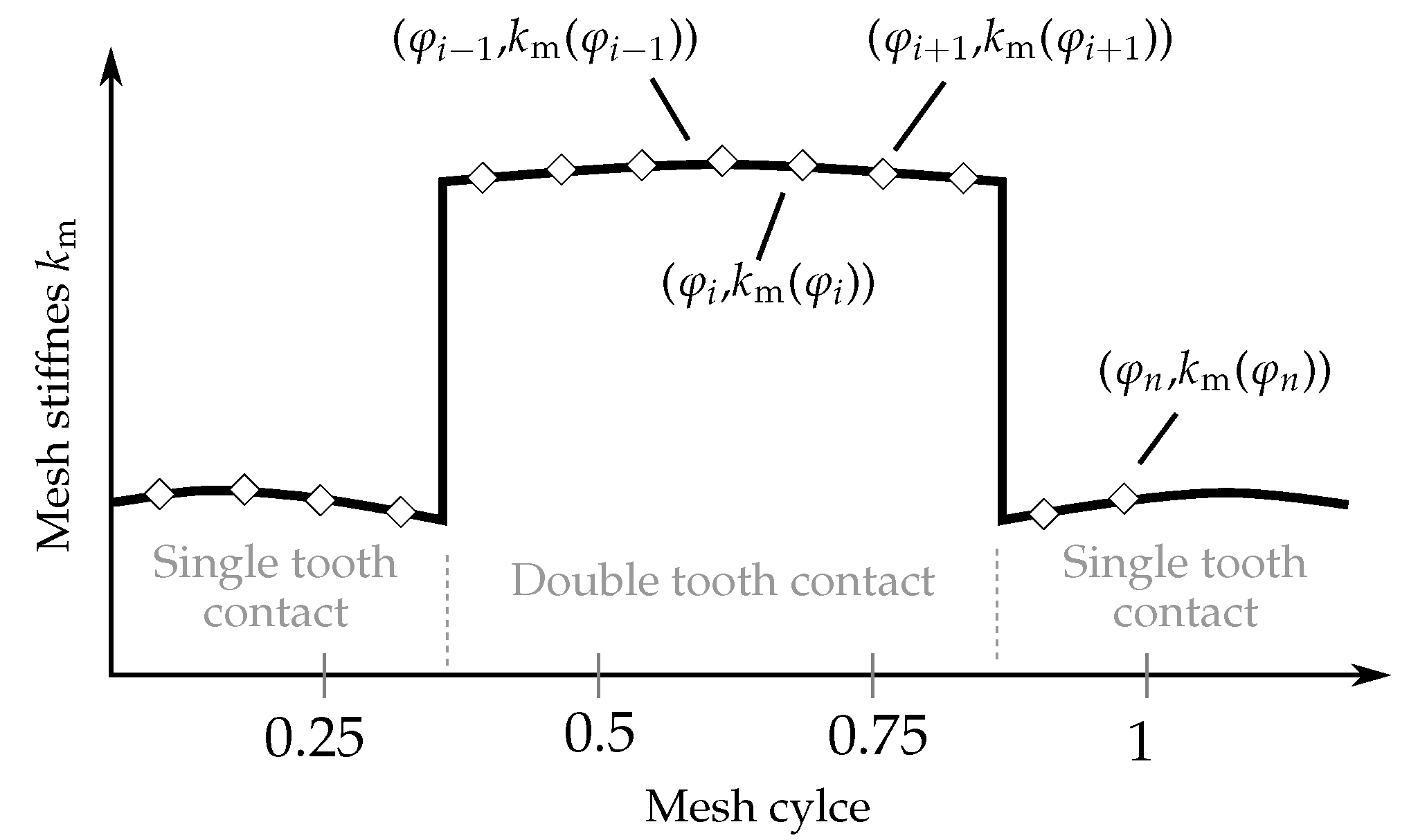
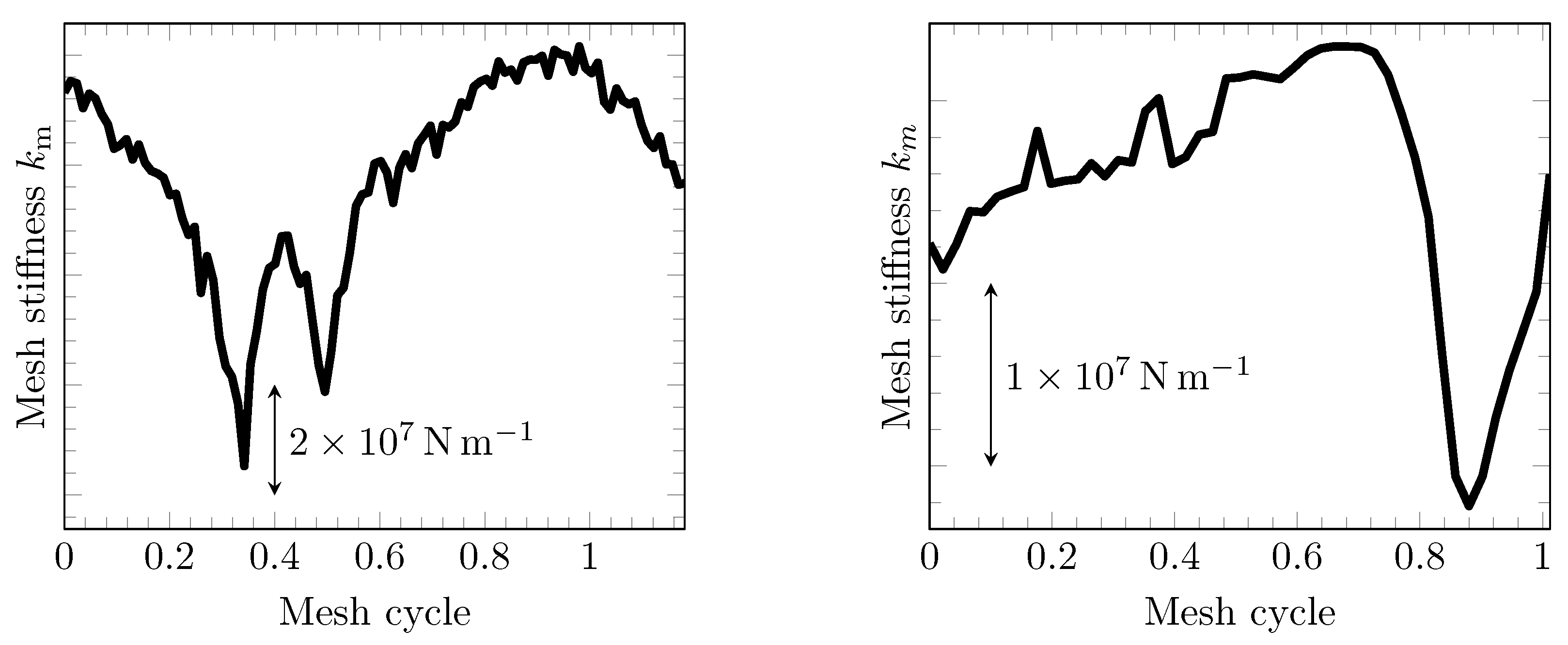
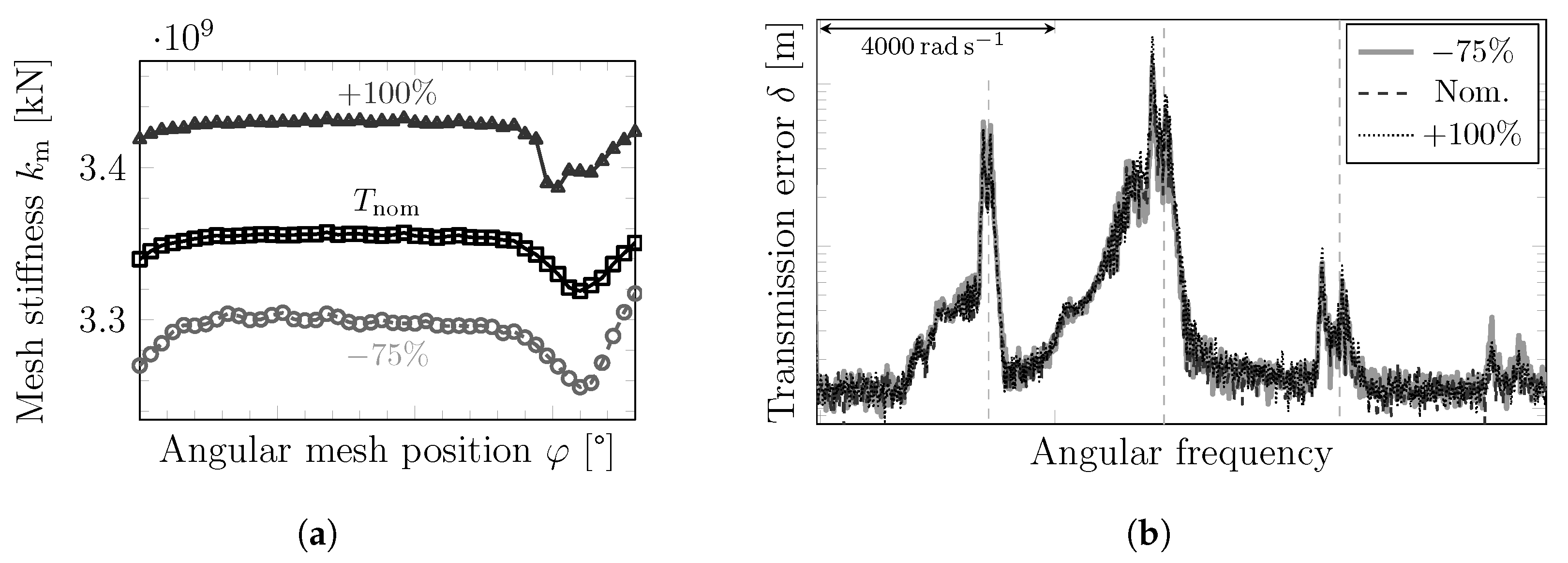
2.1. Angle-Dependent Mesh Stiffness (Step 1)

The rotation of gears in contact during operation leads to a continuous change of the instantaneous meshing configuration. Hence, the gear mesh stiffness varies continuously within a mesh cycle. This applies in principle to both spur and helical gears, although different gear properties result in different mesh stiffness fluctuations. Figure 2 compares the relative variation in the mesh stiffness over one mesh cycle for a spur and a helical gear. For better comparability, the values are related to the respective average value over one mesh cycle ${\overline{k}}_{\mathrm{m}}$. Figure 2a shows the results for the spur gear investigated by Zhou [28]. This gear has a low contact ratio (LCR), which is the standard case for spur gears. In LCR gears, the number of tooth pairs in contact varies between one and two. Therefore, the formation or loss of contact between a specific tooth pair leads to an abrupt and significant increase respectively, and decrease in the mesh stiffness. In contrast, in high contact ratio (HCR) helical gears, such as those typically used in wind turbine gearboxes (see Section 3), two or more pairs of teeth are in contact at any point in time. Hence, the load is distributed over several pairs of teeth and contact changes of individual pairs of teeth have less impact on the overall mesh stiffness. As a result, there are significantly smaller relative fluctuations in the mesh stiffness within a mesh cycle for HCR gears. Apart from these different characteristics, the angle-dependent variation in mesh stiffness is a significant cause of gear vibration in both cases. The following procedure for determining the angle-dependent mesh stiffness is equally applicable to spur and helical gear configurations.

The mesh stiffness can be determined as the slope in the non-linear force-deflection curve of mating gear teeth by either analytical, experimental or computational methods. For a discussion of the nonlinear aspects and corresponding models, see, e.g., Cooley [24].

The contact force at the tooth flanks of two mating gears is denoted as the mesh force $F_{\mathrm{m}}$. It can be calculated from the two acting torques $T_{1,2}$ and the base circle radii $r_{\mathrm{b}1,\mathrm{b}2}$ of the two gears as

$$F_{\mathrm{m}}={\displaystyle \frac{T_1}{r_{\mathrm{b}1}}}={\displaystyle \frac{T_2}{r_{\mathrm{b}2}}},$$

(1)

where the indices $1,2$ refer to the driving and the driven gear, respectively.

The mesh deflection $q_{\mathrm{m}}$ describes the displacement of the meshing gears due to elastic deformation under load, expressed as a tangential displacement at the base circle radius

$$q_{\mathrm{m}}=r_{\mathrm{b}1}{\theta }_1+r_{\mathrm{b}2}{\theta }_2-ϵ,$$

(2)

where ${\theta }_1,{\theta }_2$ denote the absolute rotational deflection of the gears and the unloaded transmission error $ϵ$ reflects relative errors between the gears due to deviations from the ideal involute shape by intentional modifications or unintentional errors, e.g., pitch, profile, pressure angle or run-out errors [11,68,69].

The mesh stiffness $k_{\mathrm{m}}$ is determined as the ratio of the mesh force $F_{\mathrm{m}}$ and the mesh deflection $q_{\mathrm{m}}$ as

$$k_{\mathrm{m}}={\displaystyle \frac{F_{\mathrm{m}}}{q_{\mathrm{m}}}}.$$

(3)

Equations (1)–(3) represent the governing equations for the mesh stiffness, which are frequently used in the literature, see, e.g., [24,28,56,70,71,72].

The angular variation of the mesh stiffness during one mesh cycle is obtained from a series of static FE computations. The FE model of a helical gear pair is shown in Figure 3. The driving gear is loaded with the torque T and the driven gear is fixed in space at the inner cylindrical surface. Contact elements are applied to the element surfaces along the tooth flanks. The FE solution provides the absolute rotational deflections ${\theta }_1$ and ${\theta }_2$ under the torque load T, so that the mesh stiffness $k_{\mathrm{m}}$ can be obtained from Equations (1) to (3) as

$$k_{\mathrm{m}}={\displaystyle \frac{T}{r_{\mathrm{b}1}·\left(r_{\mathrm{b}1}{\theta }_1+r_{\mathrm{b}2}{\theta }_2-ϵ\right)}}.$$

(4)

The mesh is refined in the zones of potential contact in order to ensure accurate contact detection and to capture small profile modifications and errors.

A number of n static simulations is performed for n equally spaced angular positions

$${\mathbf{\phi }}_{\mathrm{cycl}}={\left[{\phi }_1,\cdots ,{\phi }_i,\cdots ,{\phi }_n\right]}_{(1\times n)},$$

where the final position ${\phi }_n=2\pi /N$ equals the physical size of a mesh cycle in radians and N indicates the number of teeth on the driving gear. The simulations yield a set of n values

$${\mathbf{k}}_{\mathrm{m},\mathrm{cycl}}={\left[k_{\mathrm{m}}\left({\phi }_1\right),\cdots ,k_{\mathrm{m}}\left({\phi }_i\right),\cdots ,k_{\mathrm{m}}\left({\phi }_n\right)\right]}_{(1\times n)}$$

(5)

for the mesh stiffness. The index “cycl” refers to angle-dependent results within one mesh cycle. To illustrate the procedure, the black line in Figure 4 shows the mesh stiffness of a spur gear pair obtained with an angular resolution $n>100$. For better visibility, the markers and the notations refer to a coarse resolution with $n=13$. The approach for step 1 is intended to provide a versatile and flexible way of calculating the angle-dependent mesh stiffness $k_{\mathrm{m}}\left(\phi \right)$ for a wide range of gear types and specific gear characteristics such as pressure angle, profile modifications, gear tooth errors and similar.

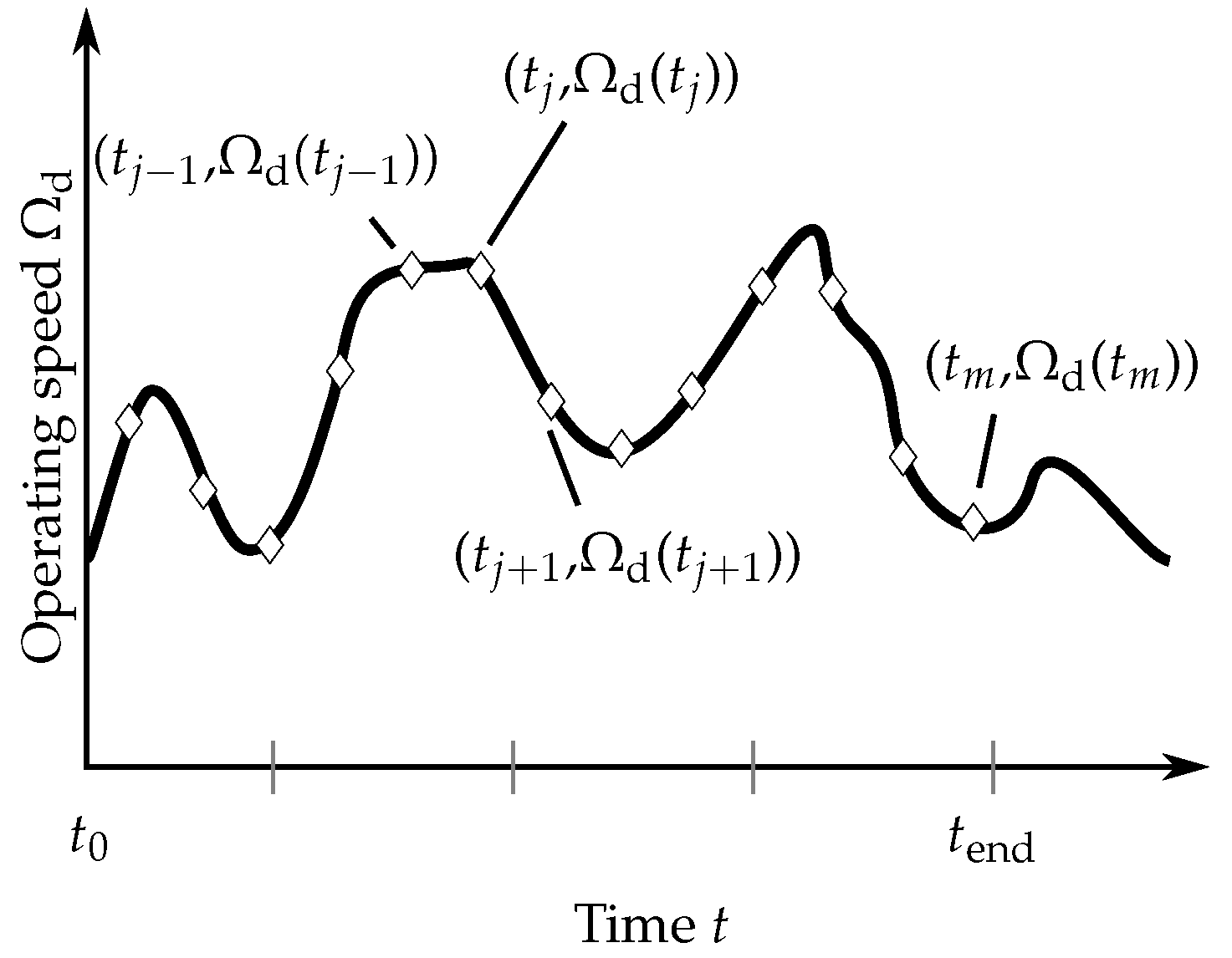
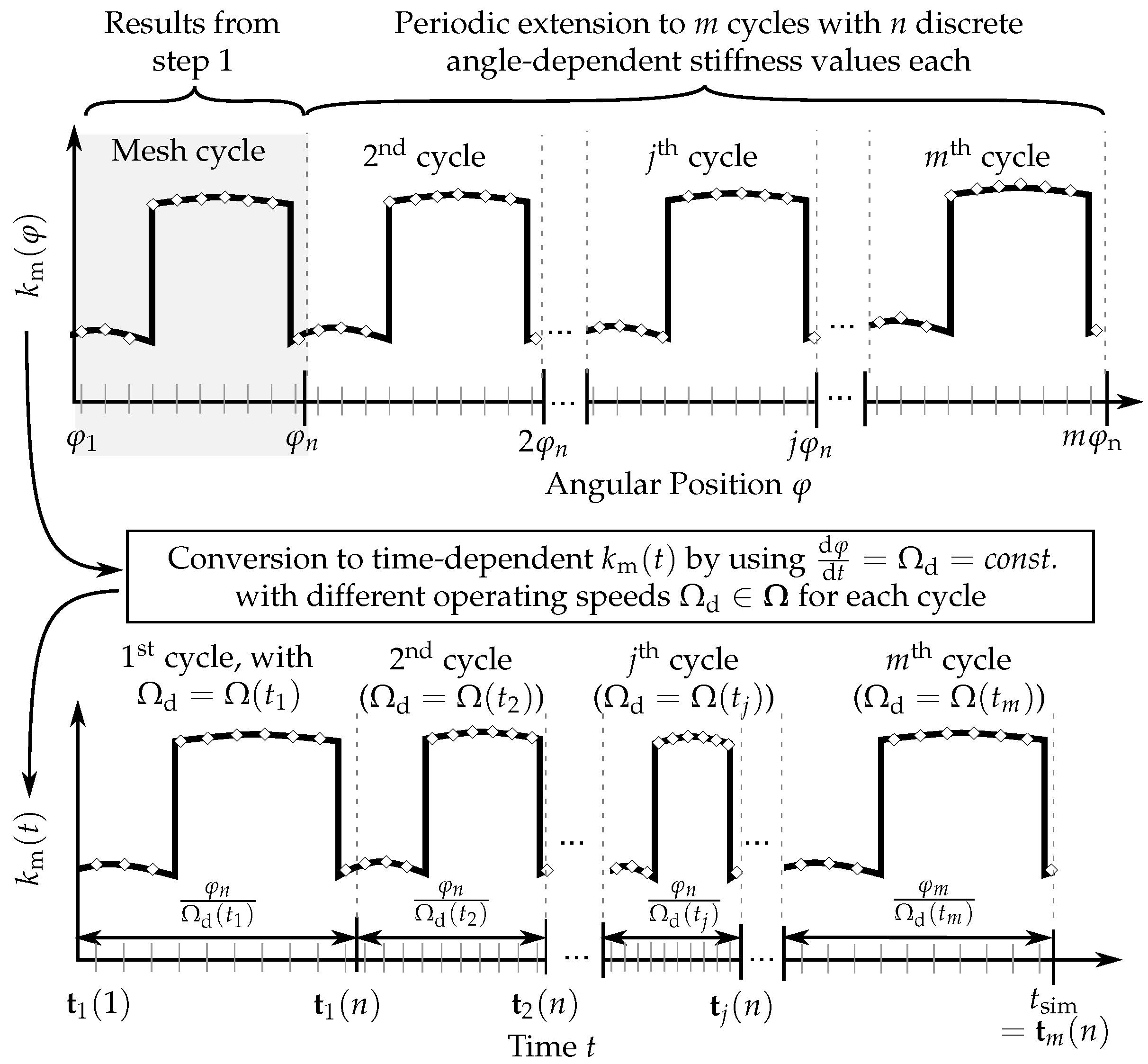
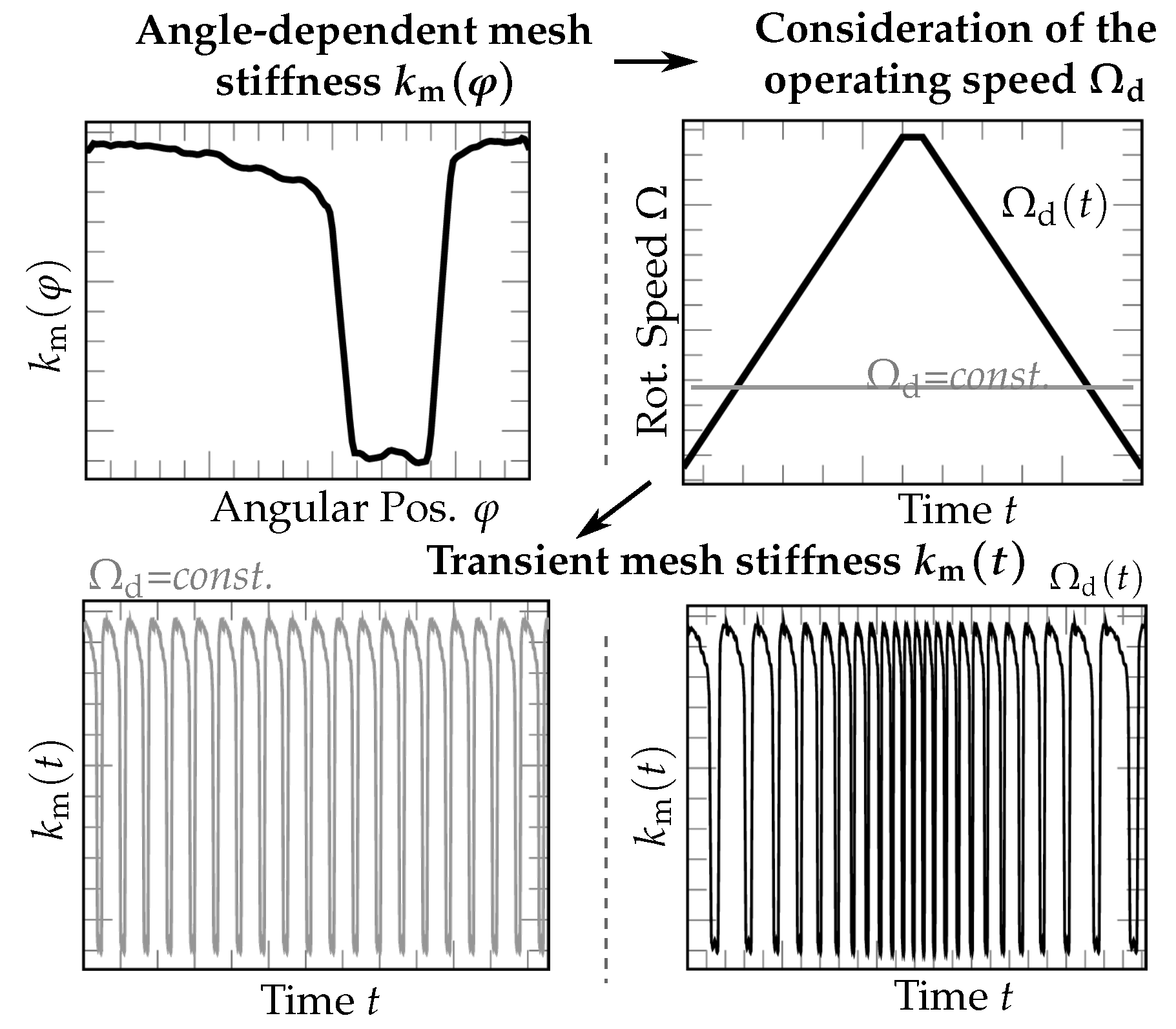
2.2. Consideration of Time-Varying Operating Conditions (Step 2)

The angle-dependent results $k_{\mathrm{m}}\left(\phi \right)$ from step 1 are used to determine the time dependence of the mesh stiffness $k_{\mathrm{m}}\left(t\right)$. For a constant operating speed ${\Omega }_{\mathrm{d}}$, the transient mesh stiffness vector for one mesh cycle ${\mathbf{k}}_{\mathrm{m},\mathrm{cycl}}\left(t\right)$ can be obtained simply as

$${\mathbf{k}}_{\mathrm{m},\mathrm{cycl}}\left(t\right)={\left[k_{\mathrm{m}}\left(t_1\right),\cdots ,k_{\mathrm{m}}\left(t_i\right),\cdots ,k_{\mathrm{m}}\left(t_n\right)\right]}_{(1\times n)},$$

(6)

with the kinematic relation ${\displaystyle \frac{\partial \phi }{\partial t}}={\Omega }_{\mathrm{d}}$, so that ${\displaystyle t_i=\frac{{\phi }_i}{{\Omega }_{\mathrm{d}}}}$. In the case of a time-varying operational speed ${\Omega }_{\mathrm{d}}={\Omega }_{\mathrm{d}}\left(t\right)$, a discrete set of operational speeds

$$\Omega ={\left[{\Omega }_{\mathrm{d}}\left(t_1\right),\cdots ,{\Omega }_{\mathrm{d}}\left(t_j\right),\cdots ,{\Omega }_{\mathrm{d}}\left(t_m\right)\right]}_{(1\times m)}$$

(7)

is extracted for m time instances, and time-varying mesh stiffness vectors according to Equation (6) are calculated for each component of $\Omega$. Figure 5 shows a distribution of the operating speeds both for a fine and a coarse resolution of the time interval. The time-dependent variation of mesh stiffness is displayed in Figure 6.

Writing the sets of angular positions ${\mathbf{\phi }}_j$ and corresponding mesh stiffnesses ${\mathbf{k}}_{\mathrm{m},\mathrm{j}}$ as row vectors, the overall result of the simulations for the whole vector $\Omega$ of operating speeds in Equation (7) can be written as a set

$${\mathbf{k}}_{\mathrm{m}}={\left[{\mathbf{k}}_{\mathrm{m},1},\cdots ,{\mathbf{k}}_{\mathrm{m},j},\cdots ,{\mathbf{k}}_{\mathrm{m},m}\right]}_{(1\times m·n)},$$

(8)

corresponding to a set of angular positions

$$\mathbf{\phi }={\left[{\mathbf{\phi }}_1,\cdots ,{\mathbf{\phi }}_j,\cdots ,{\mathbf{\phi }}_m\right]}_{(1\times m·n)},$$

(9)

where for $j>1$ the angles of rotation are augmented as

$${\mathbf{\phi }}_j=\left\{\begin{array}{cc}{\mathbf{\phi }}_{\mathrm{cycl}}\hfill & \mathrm{if}j=1\hfill \\ {\mathbf{\phi }}_{\mathrm{cycl}}+{\mathbf{\phi }}_{j-1}\left(n\right)\hfill & \mathrm{if}j>1\hfill \end{array}\right.,$$

(10)

and the vectors ${\mathbf{k}}_{\mathrm{m},j}$ are given by the results from step 1 as

$${\mathbf{k}}_{\mathrm{m},j}={\mathbf{k}}_{\mathrm{m},\mathrm{cycl}}.$$

(11)

A sequence of discrete time steps $\mathbf{t}$ corresponding to the m mesh stiffness cycles is defined as

$$\mathbf{t}={\left[{\mathbf{t}}_1,\cdots ,{\mathbf{t}}_j,\cdots ,{\mathbf{t}}_m\right]}_{(1\times m·n)},$$

(12)

where

$${\mathbf{t}}_j={\displaystyle \frac{{\mathit{\phi }}_j}{{\mathbf{\Omega }}_j}}$$

(13)

contains the time steps corresponding to the j-th mesh cycle, while it is assumed that ${\displaystyle \frac{\partial {\Omega }_{\mathrm{d}}}{\partial t}}$ is sufficiently small so that ${\Omega }_{\mathrm{d}}$ can be assumed to be constant within a mesh cycle.

As result of step 2, the time-varying mesh stiffness $k_{\mathrm{m}}\left(t\right)$ can be determined for any point in time with the discrete sets $\mathit{t}$ and ${\mathit{k}}_{\mathrm{m}}$ and linear interpolation. The conversion from angular to time-dependent mesh stiffness is illustrated in Figure 7, comparing a case of constant operating speed to a case of variable speed.

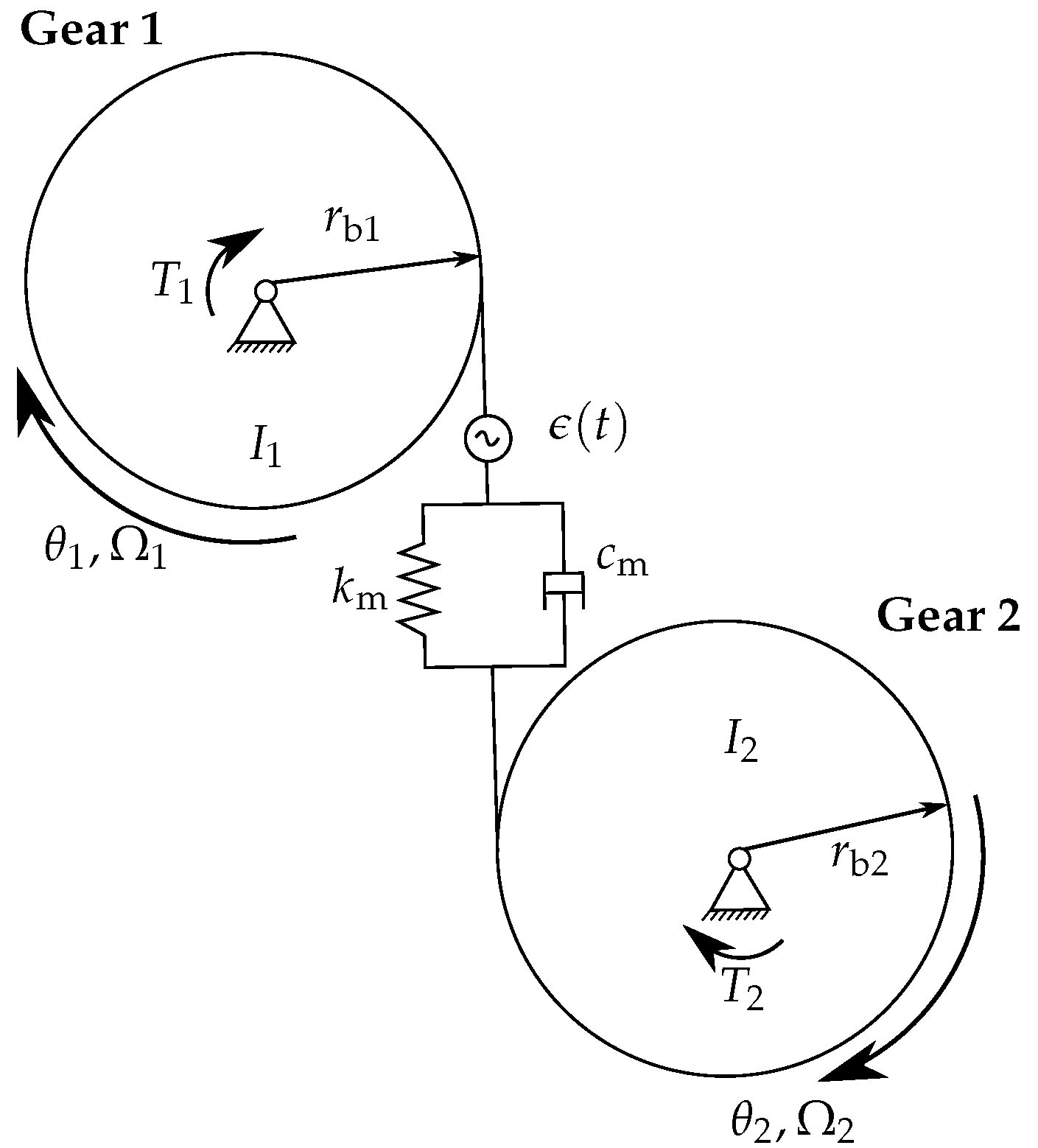
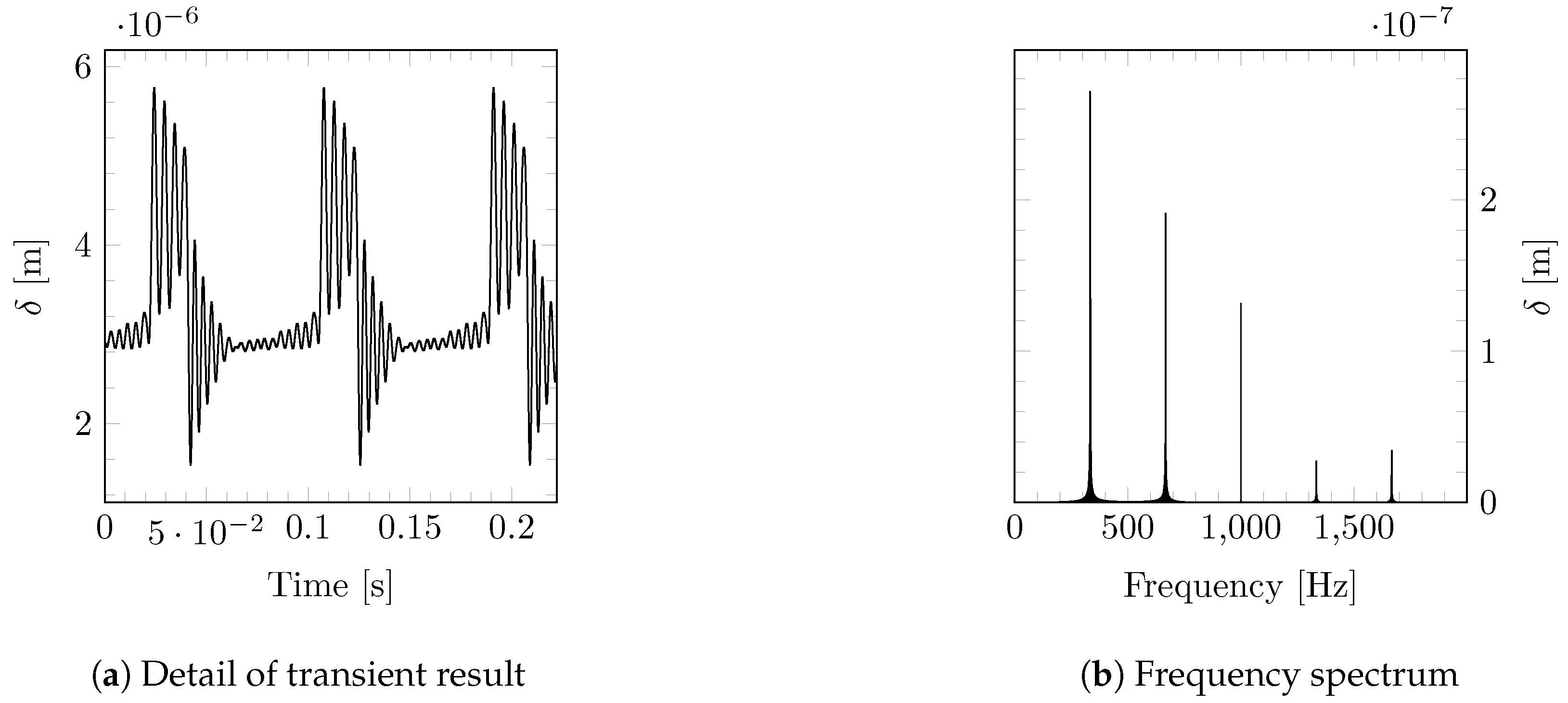
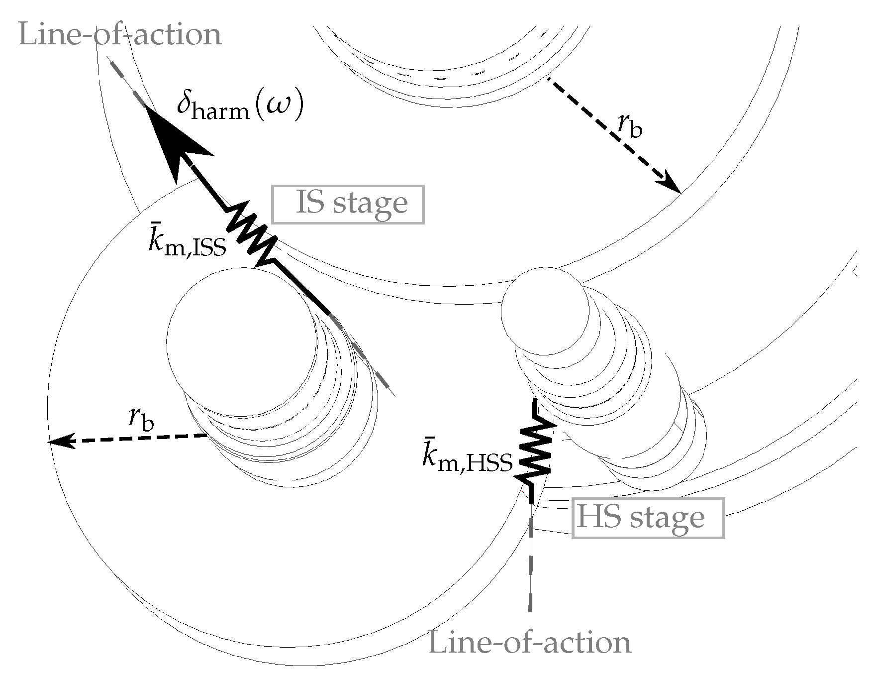
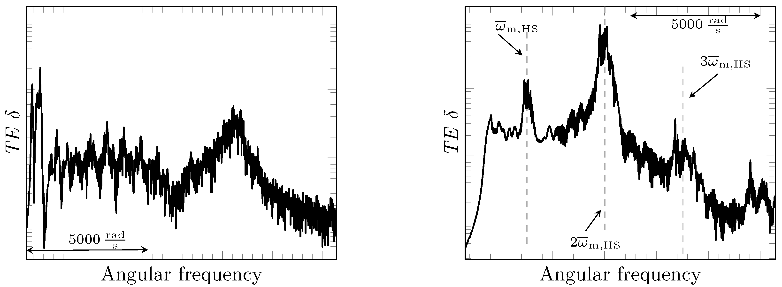
2.3. Transient Gear Dynamics (Step 3)

The time-varying mesh stiffness $k_{\mathrm{m}}\left(t\right)$ is used as input data for a two-body model of a gear pairing, shown in Figure 8. This model has been frequently used in the literature, see, e.g., [11,18,56,73,74,75,76]. It includes the most important effects of gear excitation, including varying mesh stiffness, mesh damping, and gear errors [11].

The two-body model consists of two rigid discs representing the moment of inertia of the two mating gears $I_{1,2}$ with the torsional degree of freedoms, ${\theta }_{1,2}$. The angular velocities of the vibrating discs are the sums of the rigid body velocity and the velocity of vibration, i.e., ${\Omega }_1+{\dot{\theta }}_1$ and ${\Omega }_2+{\dot{\theta }}_2$, respectively. The discs are connected at the corresponding base circle radii $r_{\mathrm{b}1,\mathrm{b}2}$ by a spring element with the mesh stiffness $k_{\mathrm{m}}\left(t\right)$, and a viscous damper representing the mesh damping with the damping coefficient $c_{\mathrm{m}}\left(t\right)$. The gears can be excited additionally by prescribed displacements due to a time-dependent unloaded transmission error $ϵ\left(t\right)$. The loads are the time-invariant driving torque $T_1$ and the driven torque $T_2$. High torque conditions are assumed, therefore the backlash is neglected. The effect of sliding friction is also neglected. The equations of motion are [65,73]:

$$\begin{array}{c}\hfill I_1{\ddot{\theta }}_1+r_{\mathrm{b}1}{c}_{\mathrm{m}}\left(t\right)\left(r_{\mathrm{b}1}{\dot{\theta }}_1+r_{\mathrm{b}2}{\dot{\theta }}_2-\dot{ϵ}\right)+r_{\mathrm{b}1}{k}_{\mathrm{m}}\left(t\right)·\left(r_{\mathrm{b}1}{\theta }_1\left(t\right)+r_{\mathrm{b}2}{\theta }_2\left(t\right)-ϵ\left(t\right)\right)=T_1\begin{array}{c}\hfill -I_1{\dot{\Omega }}_1\end{array}\end{array}$$

(14)

$$\begin{array}{c}\hfill I_2{\ddot{\theta }}_2+r_{\mathrm{b}2}{c}_{\mathrm{m}}\left(t\right)\left(r_{\mathrm{b}2}{\dot{\theta }}_2+r_{\mathrm{b}1}{\dot{\theta }}_1+\dot{ϵ}\right)+r_{\mathrm{b}2}{k}_{\mathrm{m}}\left(t\right)·\left(r_{\mathrm{b}2}{\theta }_2\left(t\right)+r_{\mathrm{b}1}{\theta }_1\left(t\right)+ϵ\left(t\right)\right)=T_2\begin{array}{c}\hfill -I_2{\dot{\Omega }}_2\end{array}.\end{array}$$

(15)

Note that the inertia terms on the right vanish for $\Omega =\mathrm{const}.$ Neglecting dissipative effects, the total energy of rigid body motion is constant, which leads to the power balance equation [34]

$$I_1{\Omega }_1{\dot{\Omega }}_1+I_2{\Omega }_2{\dot{\Omega }}_2=T_1{\Omega }_1+T_2{\Omega }_2.$$

(16)

Introducing the transmission error as

$$\delta \left(t\right)=r_{\mathrm{b}1}{\theta }_1\left(t\right)+r_{\mathrm{b}2}{\theta }_2\left(t\right)$$

(17)

and using Equations (1) and (16), the system of Equations (14) and (15) can be reduced to [65,66]

$$m_{\mathrm{e}}\ddot{\delta }+c_{\mathrm{m}}\left(\dot{\delta }-\dot{ϵ}\right)+k_{\mathrm{m}}\left(\delta -ϵ\right)=F_{\mathrm{m}}\begin{array}{c}\hfill +i{\displaystyle \frac{I_2{\dot{\Omega }}_1}{r_{\mathrm{b}2}}}\end{array}$$

(18)

with the equivalent mass ${\displaystyle m_{\mathrm{e}}=\frac{I_1{I}_2}{r_{\mathrm{b}2}^2{I}_1+r_{\mathrm{b}1}^2{I}_2}}$ and the gear ratio ${\displaystyle i=\frac{r_{\mathrm{b}1}}{r_{\mathrm{b}2}}=-\frac{{\Omega }_2}{{\Omega }_1}}$. Assuming a constant damping ratio $\zeta$, the damping coefficient is obtained as

$$c_{\mathrm{m}}\left(t\right)=2\sqrt{k_{\mathrm{m}}\left(t\right)m_{\mathrm{e}}}\zeta .$$

(19)

This approach has been widely used in the literature, see [11,28,74,77,78,79], applying damping ratios in the range from 3 to 10%.

Equation (18) is a linear ordinary differential equation in time with periodic coefficients and can be characterized as Hill equation with damping, see Cattani et al. [80]. It can be solved by standard numerical approaches. The transient solution $\delta \left(t\right)$ is then Fourier-transformed to obtain the transmission error $\delta \left(\omega \right)$ in the frequency range, where $\omega$ denotes the (angular) excitation frequency. In the final step 5 of the hybrid approach, the results for $\delta \left(\omega \right)$ are applied as an excitation spectrum to calculate the operational response spectra of the gearbox and the drive train. This approach is based on the engineering experience that gear vibrations, as a major vibrational source in industrial drive trains [11,12], which can be traced back to the transmission error at gear contact [18,19,20].

Computational results for the system discussed by Zhou et al. [28] are shown in Figure 9. The values $ϵ=0$, $\zeta =0.03$, and a constant operating speed are assumed. The transmission error $\delta$ is displayed both as a function of time and frequency. The dominant thin-banded peaks in Figure 9b occur at the constant meshing frequency ${\omega }_{\mathrm{m}}={\Omega }_{\mathrm{d}}·z$ and its multiples, where z is the number of teeth of the driving gear.

2.4. Structural Response and Transfer Behavior Using Dynamic Finite Element Analysis (Step 4)

In step 4 of the procedure, a detailed FE model of the gearbox is used for the calculation of structural dynamic transfer functions. An overview of the FE model is shown in Figure 10. The model consists of the gearbox housing and internal components, such as shafts, gears, planet carrier with shrink disc, etc. A model cutout displaying the internal components is shown in Figure 11.

The main components of the cast gearbox housing are the high speed (HS) cover, the internal gear of the planetary stage, and the torque arms, which are connected via two pins to the gearbox mounts. These mounts consist of two solid blocks per side with pins attached. Multiple elastomer layers are applied between the pins and the blocks. This setup is modeled by a 6 × 6 stiffness matrix ${\mathbf{K}}_{\mathrm{c}}$ as

$${\mathbf{K}}_{\mathrm{c}}=\left[\begin{array}{cccccc}{k}_{\mathrm{xx}}& k_{\mathrm{xy}}& k_{\mathrm{xz}}& k_{\mathrm{x}}{\theta }_{\mathrm{x}}& k_{\mathrm{x}}{\theta }_{\mathrm{y}}& k_{\mathrm{x}}{\theta }_{\mathrm{z}}\\ k_{\mathrm{yx}}& k_{\mathrm{yy}}& k_{\mathrm{yz}}& k_{\mathrm{y}}{\theta }_{\mathrm{x}}& k_{\mathrm{y}}{\theta }_{\mathrm{y}}& k_{\mathrm{y}}{\theta }_{\mathrm{z}}\\ k_{\mathrm{zx}}& k_{\mathrm{zy}}& k_{\mathrm{zz}}& k_{\mathrm{z}}{\theta }_{\mathrm{x}}& k_{\mathrm{z}}{\theta }_{\mathrm{y}}& k_{\mathrm{z}}{\theta }_{\mathrm{z}}\\ k_{{\theta }_{\mathrm{x}}}\mathrm{x}& k_{{\theta }_{\mathrm{x}}}\mathrm{y}& k_{{\theta }_{\mathrm{x}}}\mathrm{z}& k_{{\theta }_{\mathrm{x}}{\theta }_{\mathrm{x}}}& k_{{\theta }_{\mathrm{x}}{\theta }_{\mathrm{y}}}& k_{{\theta }_{\mathrm{x}}{\theta }_{\mathrm{z}}}\\ k_{{\theta }_{\mathrm{y}}}\mathrm{x}& k_{{\theta }_{\mathrm{y}}}\mathrm{y}& k_{{\theta }_{\mathrm{y}}}\mathrm{z}& k_{{\theta }_{\mathrm{y}}{\theta }_{\mathrm{x}}}& k_{{\theta }_{\mathrm{y}}{\theta }_{\mathrm{y}}}& k_{{\theta }_{\mathrm{y}}{\theta }_{\mathrm{z}}}\\ k_{{\theta }_{\mathrm{z}}}\mathrm{x}& k_{{\theta }_{\mathrm{z}}}\mathrm{y}& k_{{\theta }_{\mathrm{z}}}\mathrm{z}& k_{{\theta }_{\mathrm{z}}{\theta }_{\mathrm{x}}}& k_{{\theta }_{\mathrm{z}}{\theta }_{\mathrm{y}}}& k_{{\theta }_{\mathrm{z}}{\theta }_{\mathrm{z}}}\end{array}\right],$$

(20)

where $x,y$ are the in-plane directions and z the axis direction of the cylindrical pins, ${\theta }_{\mathrm{x}}$ and ${\theta }_{\mathrm{y}}$ denote the out-of-plane angular deflections, ${\theta }_{\mathrm{x}}$ and the angular deflection around the pin axis; see Figure 12. This description contains radial, axial, and tilting stiffness on the diagonal terms, as well as cross-coupling at the off-diagonal-terms. A diagonal 6 × 6 damping matrix

$${\mathit{C}}_c=\mathrm{diag}(c_{\mathrm{xx}},c_{\mathrm{yy}},c_{\mathrm{zz}},0,0,0)$$

(21)

is used to approximate the damping effects between pin and mount block through the elastomer.

To reduce the computational effort, the internal components are modeled as flexible bodies with simplified geometries such that the inertia and stiffness properties are correctly reflected. The rotational motion of these components and the associated dynamic effects are neglected. The internal components of the gearbox are connected by bearings to the gearbox housing. The vibration transmission behavior of these bearings has a significant influence on the propagation of gearbox vibrations into the flexible housing and other connected components. Since it is not possible to include detailed FE models of each bearing, reduced-order models are applied. For each bearing position, the shaft and the housing bearing support surface are assumed to be rigid. All nodes on these surfaces are connected separately with rigid body elements (RBE). The independent nodes are described with six DoFs each, see Figure 12. Several studies have demonstrated that the cross-coupling effects in bearings have a significant impact on the vibration transmission in gearboxes [81,82]. Therefore, the translational and rotational DOFs in the independent nodes of either RBE are coupled by 5 × 5 stiffness matrices ${\mathbf{K}}_{\mathrm{b}}$ for each bearing connection, as discussed in, e.g., [83]. The matrices ${\mathbf{K}}_{\mathrm{b}}$ are defined analogously to ${\mathbf{K}}_{\mathrm{c}}$ in Equation (20), except that they do not contain stiffness components related to the bearing axis. The entries of the stiffness matrices ${\mathbf{K}}_{\mathrm{b}}$ and ${\mathbf{K}}_{\mathrm{c}}$ can be obtained by experimental measurements or detailed numerical submodels of the mounts and bearings.

Özgüven has shown in [11], that the analytically calculated gear excitation can be introduced to the dynamic simulation of gears in contact by combining a constant mesh stiffness with a displacement excitation at the contact point. In the FE model, the gears are therefore approximated by circular discs whose radii are equal to the base circle radii $r_{\mathrm{b}}$. The gear contact of each gear pairing is represented by spring elements that are attached to the gears along the line-of-action, as shown in Figure 13. The spring elements are equipped with the averaged stiffness

$${\overline{k}}_{\mathrm{m}}={\displaystyle \frac{z}{2\pi }}{\int }_0^{\frac{2\pi }{z}}{k}_{\mathrm{m}}\left(\phi \right)\mathrm{d}\phi ,$$

(22)

where $\phi$ is the angular position in the mesh cycle and z is the number of teeth.

In order to represent the vibration excitation that emerges from the gears under operating conditions, the gearbox is excited by a small displacement amplitude in the direction of the transmission error. Thus, at each stage s, the structure is excited by a lateral displacement

$${\delta }_{\mathrm{harm},}s=c_s·e^{\mathrm{i}\omega t}\mathrm{for}\omega \in {\mathbb{R}}^{+},$$

(23)

with $\left|c_s\right|\ll r_{\mathrm{b},s}$ in order to satisfy the assumption of small displacements. In the same way, transfer functions are computed for all gear stages that are considered as potential excitation sources for the vibroacoustic simulation.

The size of the finite elements is adapted to the highest frequencies of interest in order to guarantee a numerically sufficient resolution of the bending waves in the gearbox housing. A coarser mesh density is sufficient for the internal parts.

Assuming a time-harmonic excitation with driving frequency $\omega$, the complex-valued nodal amplitudes $\widehat{\mathit{u}}$ of the FE model can be determined for steady-state conditions from the linear algebraic system

$$\left(\mathit{K}-{\omega }^2\mathit{M}+i\omega \mathit{C}\right)\widehat{\mathbf{u}}=\widehat{\mathit{f}},$$

(24)

where $\mathit{K}$, $\mathit{C}$, and $\mathit{M}$ denote the time-invariant stiffness, damping, and mass matrix. The vector of complex-valued load amplitudes $\widehat{\mathit{f}}$ contains pseudo-force terms originating from the non-zero prescribed displacements corresponding to the transmission error, see the standard references [84,85] for details. It is assumed that nonlinear parameters have been linearized around the operating point. The time-harmonic solution of Equation (24) is significantly less expensive than a transient simulation for comparable model size, as has been shown in [86].

The dynamic FE simulations are used to obtain transfer functions

$$H_{sr}(i\omega )={\displaystyle \frac{Y_{\mathrm{harm},}r(i\omega )}{{\delta }_{\mathrm{harm},}s(i\omega )}},$$

(25)

where ${\delta }_{\mathrm{harm},}s(i\omega )$ denotes the complex amplitude of the imposed displacement at DoF s in Equation (23), and $Y_{\mathrm{harm},}r(i\omega )$ is the frequency response of a result quantity r obtained from the solution of Equation (24) over a frequency band.

The presented FE modeling approach is also suitable for the application of component mode synthesis (CMS) reduction techniques, which can provide a further reduction of the calculation effort [87].

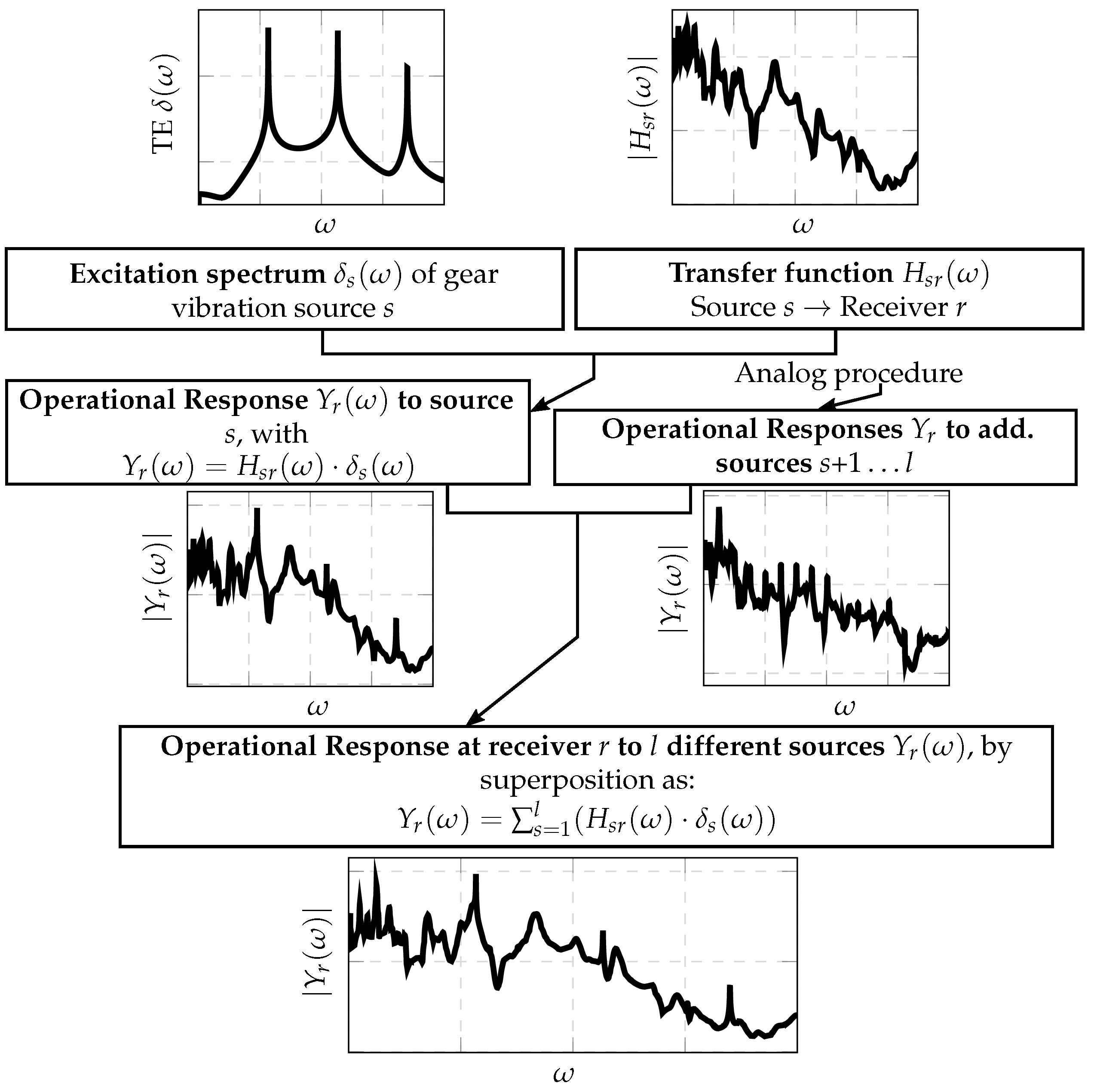
2.5. Response at Operating Conditions (Step 5)

The dynamic response spectra to specific operating conditions is calculated by an analytical combination of precomputed excitation spectra and transfer functions. The procedure for single and multistage gear excitation is shown in Figure 14. The response under operating conditions is computed using the excitation spectra ${\delta }_s\left(\omega \right)$ from Equation (18) and the transfer functions $H_{sr}(i\omega )$ from Equation (25). The response spectrum $Y_r\left(\omega \right)$ of any linear response quantity r (e.g., dynamic displacement, velocity or acceleration) to an excitation by the s-th gear stage is given by

$$Y_r\left(\omega \right)=H_{sr}(i\omega )·{\delta }_s\left(\omega \right).$$

(26)

In case of multiple gear vibration sources, the procedure is performed for every source separately. The operational response $Y_r(i\omega )$ to an excitation by l gear stages is then calculated by superposition

$$Y_r(i\omega )=\sum _{s=1}^l{H}_{sr}(i\omega )·{\delta }_s(i\omega ),$$

(27)

where the phase shifts ${\varphi }_{\delta ,s}$ between the gear excitations at the separate stages are included in the complex amplitudes as

$${\delta }_s(i\omega )=Re\left\{\right|{\delta }_s\left(\omega \right)\left|·e^{i(\omega t+{\varphi }_{\delta ,s})}\right\}.$$

(28)

3. Numerical Results and Experimental Validation

The hybrid multistep approach of vibroacoustic simulation is applied to a multi-stage wind turbine, and computational results are compared to experimental data. The vibroacoustic measurements were carried out in an Indian semi-desert on a $2.5$ $\mathrm{M}$$\mathrm{W}$ wind turbine in full operation. Correspondingly, the computational model encompasses the complete drive train, including the rotor hub and the generator, the main bearing, mainframe and girder, and the nacelle. The evaluation and validation in this paper is focused on gearbox vibrations.

3.1. Application of the Integrated Computational Procedure

In the first step of the integrated computational procedure, the mesh stiffness is calculated for the helical intermediate and high speed stages at $n=75$ equidistant angular positions within a mesh cycle. The wind turbine also contains a planetary gear stage, but experience [10] has demonstrated that the vibro-acoustic response is dominated by the intermediate and high speed stages.

The angle-dependent mesh stiffness results are shown in Figure 15. Since the IS and HS gear stages are high-contact-ratio helical gear stages, the fluctuation of the mesh stiffness over a mesh cycle is significantly lower and less rapid than for spur gears.

The angle-dependent mesh stiffness from step 1 is transformed to TVMS in step 2 of the integrated procedure, which are then used in step 3 as input for the transient two-body model simulation of gear contact. In step 2, the operating conditions are represented by a set of $m=480$ discrete operating speeds. Hence, the transient mesh stiffness $k_{\mathrm{m}}$ is defined for $m=480$ mesh cycles according to Equations (7)–(12).

Within step 3, Equation (18) is solved with the explicit forth order Runge-Kutta scheme. The unloaded TE $ϵ$ is neglected. The calculated results for the TE excitation spectra for both the IS and HS stage are shown in Figure 16. The TE spectrum of the IS stage contains a number of frequency peaks that can be associated with the gear mesh orders of this stage. None of these peaks are dominant enough to be a possible reason of tonal effects in the radiated spectrum. The spectrum of the HS stage is characterized by three dominant peaks at the meshing frequency ${\omega }_{\mathrm{m},\mathrm{HS}}$ and its first two multiples. The vertical lines indicate the average mesh frequency of the HS stage ${\overline{\omega }}_{\mathrm{m},\mathrm{HS}}$ and its multiples. The average frequency is related to the average operating speed of the HS stage ${\overline{\Omega }}_{\mathrm{d}}$ by

$${\overline{\omega }}_{\mathrm{m},\mathrm{HS}}={\overline{\Omega }}_{\mathrm{d}}·z,$$

(29)

where z denotes the number of teeth on the HS driving gear. Previously published experience [10] shows that most tonalities in the radiated spectrum can be traced back to the first few orders of the HS stage mesh frequency. The results obtained in this work, both from measurements and the computational procedure, confirm this effect, which underlines the special significance of the frequency ranges around ${\overline{\omega }}_{\mathrm{m},\mathrm{HS}}$ and their first few multiples.

Comparing to the results at constant speed in Figure 9b, the peaks of the present response are more broadband, since the values of the instantaneous meshing frequencies ${\omega }_{\mathrm{m},\mathrm{IS}}$ and ${\omega }_{\mathrm{m},\mathrm{HS}}$ and their multiples vary with time.

In step 4, the dynamic FE simulations are performed based on the FE model shown in Figure 10 and Figure 11. The FE model of the gearbox is fixed to the ground on the bottom side of the gearbox mounts. The internal components are connected by 14 rolling-element-bearings to the gearbox housing (two each at the planet carrier, at LS shaft, at IS shaft, at HS shaft, and at the three planet shafts). The components of the stiffness matrix ${\mathit{K}}_{\mathrm{c}}$ for the mounts were determined from experimental data, while the components of the stiffness matrix ${\mathit{K}}_{\mathrm{b}}$ for the bearings were obtained from computational simulations with detailed FE models of the bearings. The internal components are modeled with average element lengths of 6 mm, while the average element length of the housing parts is 3 mm. The model order is reduced by creating superelements with the Craig-Bampton method. The model is simulated separately for excitations at the IS and HS stage, resp., with excitation frequencies $\omega$ from 0 to 12,570 $\mathrm{rad}$ ${\mathrm{s}}^{-1}$ using a step size $\Delta \omega =2\pi$ $\mathrm{rad}{\mathrm{s}}^{-1}$.

The final step 5 of the integrated procedure involves the analytical computation of the vibrational response to true operating conditions, combining the results of steps 3 and 4 in Equation (27) with $l=2$ gear sources. The computational results are discussed and compared to experimental results in the following subsection.

3.2. Computational Costs

In this subsection, some benchmark analysis is presented for the $2.50$ $\mathrm{M}$$\mathrm{W}$ WT gearbox.

Table 1. Computational time required for each step of the integrated procedure for an application to a $2.5$ $\mathrm{M}$$\mathrm{W}$ wind turbine gearbox.

Step	Analysis Task	Method	Time
1	Angle-varying mesh stiffness	Static FEM	10 $\min$
2	Time-varying mesh stiffness	Analytical	$0.5$ $\mathrm{s}$
3	Transmission Error (TE)	Runge-Kutta scheme	10 $\mathrm{s}$
4	Frequency Response	Time-harmonic FEM	$61.1$ $\min$
5	Linear Combination and Superposition	Analytical	$12.1$ $\mathrm{s}$

shows the computational time required for each step of the procedure on a PC workstation equipped with two Intel XEON Gold 5115 CPU v2 (10 cores, 20 threads, $2.40$ $\mathrm{GHz}$ each), a memory of 192 $\mathrm{GB}$ RAM, and an SSD hard drive. All FE simulations were performed using the commercial software Ansys 2020 R2.

The FE models for the calculation of the angle-varying mesh stiffness in step 1 consist of approx. four million quadratic tetrahedral elements with 1.78 × 10⁷ DoFs in both stages. Mesh sizes were determined by examining the convergence of the rotational deflection, with a particular focus on the regions of potential contact with significantly smaller element sizes. The average duration of the calculation is about 10 minutes per angular position, using preconditioned conjugate gradient solvers and parallel computations on 16 cores. As described above, both gear stages are analyzed in 75 equidistant angular positions, with a total computational time of approx. 25 $\mathrm{h}$ for the 150 separate FE simulations. The computational time to obtain the TVMS for varying operational speeds in step 2 amounts to about $0.5$ $\mathrm{s}$. The transient simulation of the gear dynamic model in step 3 takes approx. 10 $\mathrm{s}$. The FE model of the gearbox structure in step 4 consists of 463,034 quadratic hexahedral, tetrahedral, and wedge elements with 796,539 nodes and 2.39 × 10⁶ DoFs in total. The mesh sizes were determined here by evaluating the quantitative assurance of the operational deflection results for each frequency response with a reference model with very fine mesh size (2,227,510 nodes). This new approach will be described in more detail in a future publication. The time-harmonic analysis is performed for TE excitation at IS and HS stage with 2000 frequency increments each. The solution of the reduced FE model requires $6.70$ $\mathrm{GB}$ RAM and $40.50$ $\min$ of computing time, while using distributed sparse matrix direct solvers and parallel computations on 16 cores. The creation of the reduced model takes additional $26.25$ $\min$. In the fifth step, the calculation and output of the operational response spectra for 84 considered degrees of freedom takes about $12.09$ $\mathrm{s}$. From the above, it can be observed that the execution of the entire proposed sequential procedure has a total duration of approx. $26.80$ $\mathrm{h}$ for the presented benchmark analysis.

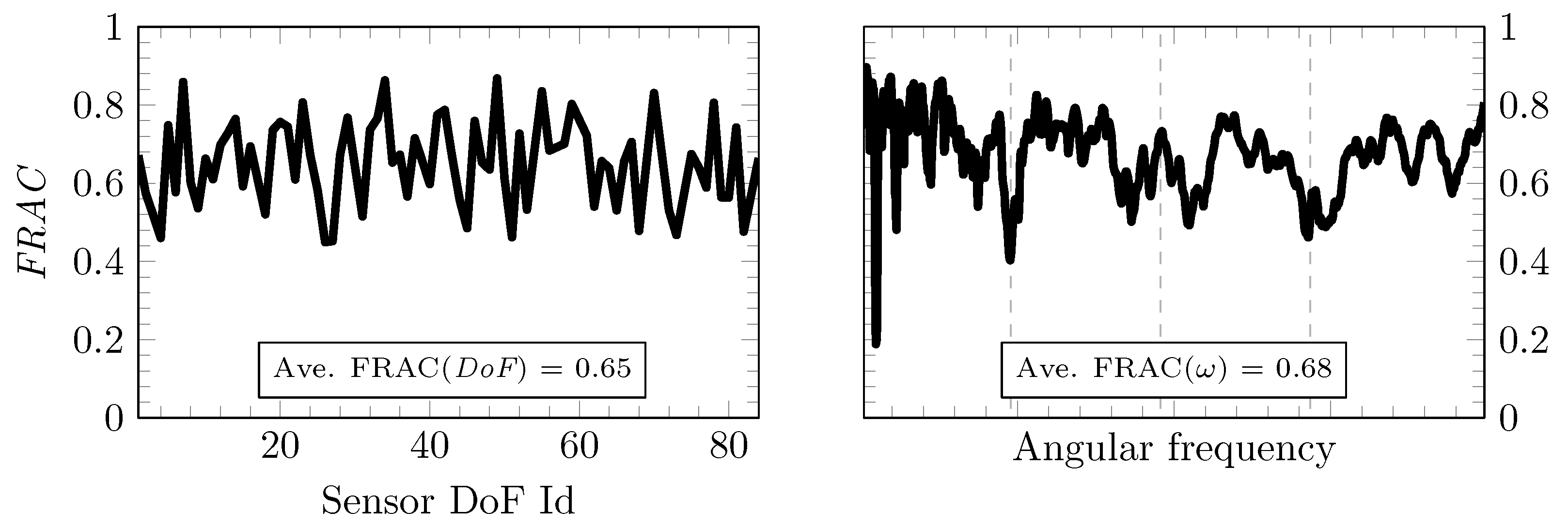
3.3. Comparison with Measurements

Multiple accelerometers were distributed on the gearbox housing and mounts; see Figure 17. Acceleration response spectra were obtained from 186 transient acceleration signals during regular operation. To cover as many positions as possible, multiple measurement runs with changing sensor positions and one permanent reference sensor were carried out. The operating speeds were recorded with a sampling frequency of 1 Hz.

The calculated and measured operational response spectra are compared in detail for a representative selection of sensor positions (SP); see Figure 18. SP A is close to a bearing seat of the HS stage and in close proximity to the vibration sources. SP B is located centrally on the top of the HS cover. SP C lies on the opposite side to the vibration sources, while SP D is situated at the top of the ring gear close to the planetary stage. The SP E and SP F are located on the back and front side of the gearbox, respectively. The structure-borne sound path between these SPs and the vibration sources is significantly longer than the paths from the SPs A to D. The locations for SP G and SP H are close to the interface between the torque arms and gearbox mounts. SP G is on the pin and SP H is located on the top of a mount. Hence, the transfer path between the vibration sources and SP H runs through the elastomer damping elements, which were modeled using 6 × 6 coupling matrices. For each SP, the acceleration in one specific direction is considered, i.e., in x-direction for SPs E,F, and G, y-direction for SP A, and z-direction for SPs B,C,D, and H, where the axial directions refer to the reference coordinate system at the reference sensor R, as shown in Figure 18. The temporal variation of the operating speeds during the different runs is displayed in Figure 19.

In this subsection, the results for the first run are discussed, while in the following subsection the influence of different operating conditions is evaluated. The spectra for the SPs A to H are shown in Figure 20. Both measurement and model results show several conforming properties across all spectra. In all cases, the major response peaks are “smeared out” around ${\overline{\omega }}_{\mathrm{m},\mathrm{HS}}$ and $2{\overline{\omega }}_{\mathrm{m},\mathrm{HS}}$. The peak at $3{\overline{\omega }}_{\mathrm{m},\mathrm{HS}}$ is lower and broader.

In general, the response spectra obtained with the hybrid multistep approach are in good agreement with the measured spectra in terms of the absolute magnitudes and qualitative comparison. All results are displayed at their absolute magnitudes, without any scaling or normalizing. The model results correspond particularly well with the measurements at the most dominant peaks around $2{\overline{\omega }}_{\mathrm{m},\mathrm{HS}}$, regarding both the magnitude and the width of the peak. The agreement of the peak magnitudes is less satisfactory at the average meshing frequency ${\overline{\omega }}_{\mathrm{m},\mathrm{HS}}$, except for the SPs B and C. The broadband peak in the range of $3{\omega }_{\mathrm{m},\mathrm{HS}}$ is also calculated in good agreement with the measurements for all SPs. Regarding the high-frequency range above $3{\overline{\omega }}_{\mathrm{m},\mathrm{HS}}$, the computed response level is significantly lower than the measured one. It should be noted that the simulations consider only the gear-induced vibrations, while the measurements contain also the effect of generator-induced vibrations, which typically occur in the high-frequency range.

The agreement between calculated and measured spectra is quantified using the frequency response assurance criterion (FRAC), which is an established frequency-domain correlation criterion [88,89] defined as

$$\mathit{FRAC}={\displaystyle \frac{|{\mathbf{Y}}_{\mathrm{b}}^{\mathrm{H}}{\mathbf{Y}}_{\mathrm{a}}{|}^2}{\left({\mathbf{Y}}_{\mathrm{b}}^{\mathrm{H}}{\mathbf{Y}}_{\mathrm{b}}\right)\left({\mathbf{Y}}_{\mathrm{a}}^{\mathrm{H}}{\mathbf{Y}}_{\mathrm{a}}\right)}},$$

(30)

where ${\mathbf{Y}}_{\mathrm{a}}$ and ${\mathbf{Y}}_{\mathrm{b}}$ denote two column vectors of response spectrum values. The FRAC values can be computed either as a function of the measured DoFs or as a function of the measured frequencies. In the first case, ${\mathbf{Y}}_{\mathrm{a}}$ and ${\mathbf{Y}}_{\mathrm{b}}$ contain the data for all measured frequencies in successive order and the scalar products in Equation (30) are computed for each DoF, while in the second case, the data are reshaped into a column vector containing all DoFs and the scalar products are computed for each frequency.

A comprehensive assessment of the obtained results is achieved by considering the FRAC for all SPs covered in the first run. For each SP, the response spectra along all three axes are taken into account. Therefore, the FRAC is evaluated in dependence to the model degrees of freedom, which are associated with measured acceleration signals, see Figure 21 (left). As a function of the DoF, the FRAC values vary in the range from 0.5 to 0.9 with an average FRAC of 0.7. Referring to the FRAC values indicated in Figure 20 it is concluded that the SPs A-H are representative for the correlation of measurement and computation in all SPs.

Subsequently, the dependence of the FRAC value on the frequency is evaluated; see Figure 21 (right). Again, the response spectra in all three spatial directions for all SPs covered in the first run are considered. The FRAC values vary between approx. 0.6 and 0.8 over wide ranges of the frequency range. The average over the frequency range is 0.7. A major decrease in correlation is observed at the average meshing frequency ${\overline{\omega }}_{\mathrm{m},\mathrm{HS}}$. This corresponds to the underestimation of the frequency peak in this range. Smaller decreases in the FRAC-values can be found around the multiples of the average mesh frequency $2{\overline{\omega }}_{\mathrm{m},\mathrm{HS}}$ and $3{\overline{\omega }}_{\mathrm{m},\mathrm{HS}}$.

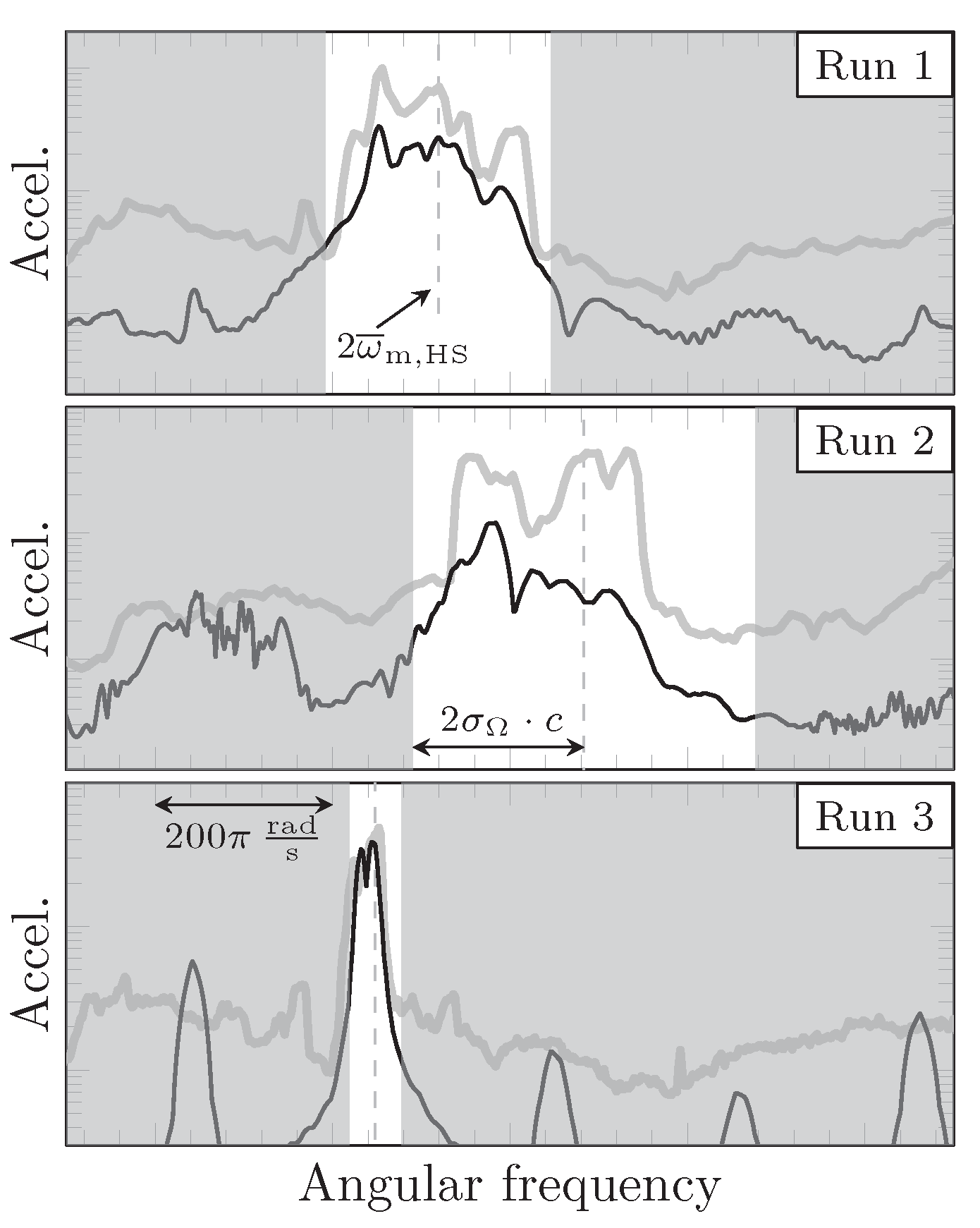
3.4. Influence of Varying Operating Conditions

Gear systems in operation are subject to variations of their torque load and angular velocity. The influence of these variations on the vibrational response is explored in the present subsection. Regarding the load level, it is well known that the size of the contact areas, and hence the mesh stiffness, may change significantly with the torque magnitude [24]. To check the sensitivity of the present gear setting, the mesh stiffness was computed for different loads T ranging from $-75\%$ to + 100% compared to the nominal operating torque $T_{\mathrm{nom}}$. The mesh stiffness results within a mesh cycle for these different loads are shown in Figure 22a, where the relative difference to the results for $T_{\mathrm{nom}}$ ranges between +2.2% and −1.6%. The variation of the mesh stiffness over a mesh cycle is very similar for all torques.

In order to evaluate the effect of varying load levels on the frequency response, Equation (18) is solved for each load case while all parameters are identical except that $k_{\mathrm{m}}$ corresponds to the results obtained for each specific load. The results for the TE excitation spectra are shown in Figure 22b. It can be observed that different meshing stiffnesses do not have a significant effect on the excitation spectrum $\delta \left(\phi \right)$ of the dominant high-speed gear stage.

However, the characteristics of the response spectra depend significantly on the variation of the operational speed. Meanwhile, steep peaks or “needles” are observed in the response to constant speed (cf. Figure 9b); the peaks are smeared out around the average meshing frequencies for varying speeds in Figure 20. This observation is confirmed in Figure 23, which shows details of the operational spectra around the dominant peak at $2{\overline{\omega }}_{\mathrm{m},\mathrm{HS}}$. Here, the measured and computed spectra at the reference sensor R are compared over a range of parse-numbers = false $1000 \pi$ $\mathrm{rad}$ ${\mathrm{s}}^{-1}$ for the different environmental conditions in the test runs 1–3. The focus is on the dominant peak around $2{\overline{\omega }}_{\mathrm{m},\mathrm{HS}}$ and its dependence to the different operating speeds, which fluctuated significantly during the first and second run, while calm wind conditions lead to a relatively constant low-level speed during the third run. The mean values ${\overline{\Omega }}_{\mathrm{d}}$, standard derivation ${\sigma }_{\Omega }$ and range $R_{\Omega }$, all being highest in the second and lowest in the third run, are shown in

Table 2. Operating speeds ${\Omega }_{\mathrm{d}}$ of the HS stage during measurement runs 1–3, regarding mean value ${\overline{\Omega }}_{\mathrm{d}}$, standard derivation ${\sigma }_{\Omega }$, and range $R_{\Omega }$.

Run	${\overline{\Omega }}_{\mathbf{d}}$	${\mathit{\sigma }}_{\Omega }$	${\mathit{R}}_{\Omega }$
	[${\mathbf{min}}^{-1}$]	[${\mathbf{min}}^{-1}$]	[${\mathbf{min}}^{-1}$]
1	290.1	9.6	42.3
2	315.7	14.6	48.2
3	280	0.6	2.2

. The mean values and the standard deviation are highlighted in the response spectra of Figure 23. The coefficient c accounts for the conversion from the average operating speed (in RPM) to the second order meshing frequency (in $\mathrm{rad} {\mathrm{s}}^{-1}$) of the HS stage. Within the proposed integrated procedure, only step 2 needs to be adapted in order to calculate the TVMS for the different environmental conditions.

The relatively constant operating speed in the third run corresponds to a narrow-banded frequency peak at $2{\overline{\omega }}_{\mathrm{m},\mathrm{HS}}$, both in the physical measurement and computational simulation. In comparison to run 3, the peaks around the second order meshing frequency of the HS stage are more broad banded for runs 1 and 2. This effect of ”frequency smearing”, which corresponds to the speed fluctuation during these two runs, is clearly visible both in the measured and in the computed spectra. Moreover, the comparison of the plot reveals the frequency shift of the average frequency, corresponding to the different average speeds in the second column of Table 2. The measured and computed spectra are in good agreement regarding this effect. The simulated spectrum of the third run (for a relatively small and constant operational speed) shows small-banded peaks at the first five gear mesh orders. Except for the second order, these peaks do not appear in the measured spectrum. This can be possibly explained by masking effects from structural noise sources other than gear noise. It should be noted that the measurements were carried out in an industrially operated WT, and hence the measured spectrum contains the combined effect of all vibrational sources on the drive train, whereas the simulation considers only the meshing errors of the two major gear stages as sources of gearbox vibrations.

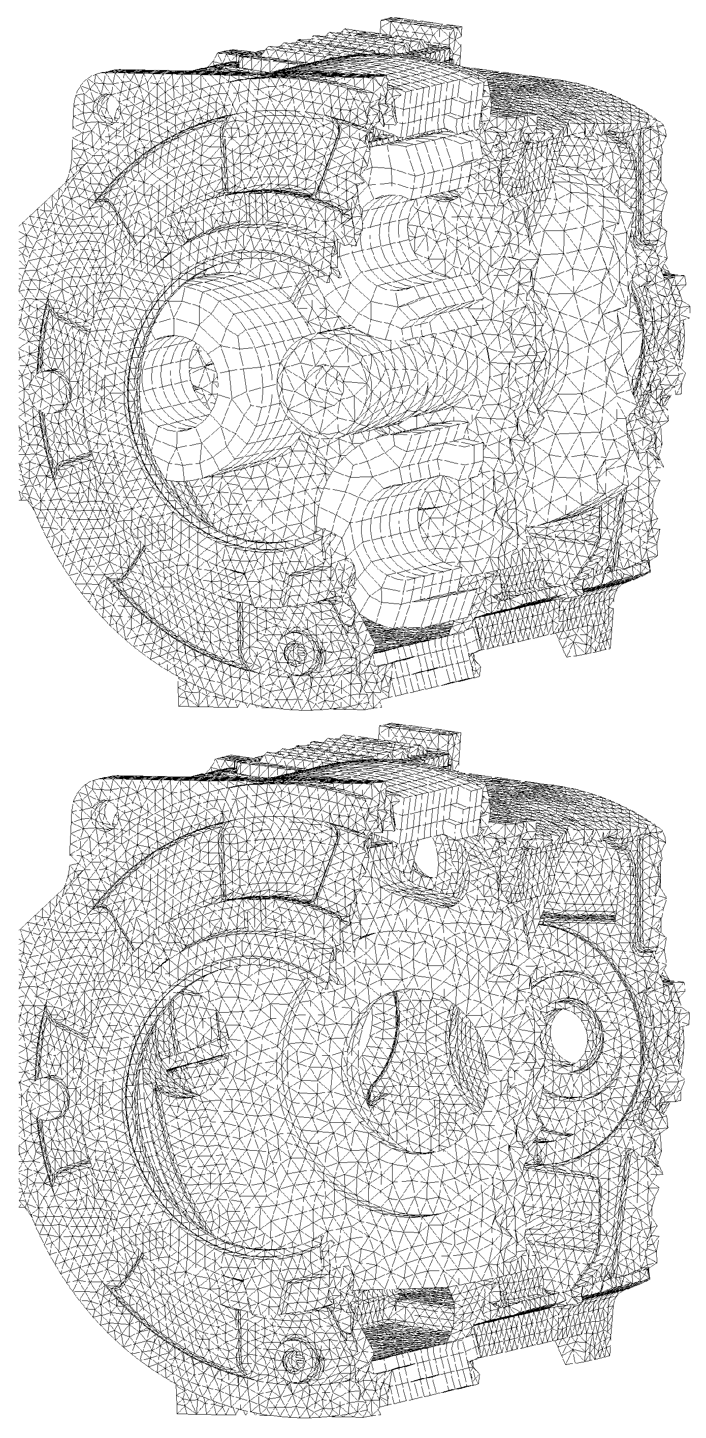
3.5. Influence of the Internal Components

The FE gearbox model contains coarse submodels of the internal components, which are often neglected in the literature. In this subsection, the response functions of the full model are compared to those of a reduced model that does not contain the internal components. Both configurations are equally excited by a unit bearing force along the line-of-action distributed over the surfaces of the bearing seat on the rotor-side bearing of the HS shaft. The details of either modeling approach are displayed in Figure 24, and the resulting frequency spectra are compared in Figure 25 at six measuring points, A–F.

Clearly the influence of the internal components on the resonance spectrum increases with the distance of the SP from the sound source. The curves are almost identical over the whole range in SP A, which is situated closest to the vibrational source. The farther the SP position is from the excitation source, the larger the discrepancy between the response spectra of the full and the reduced model become. Although the results are relatively similar in all cases at the medium frequencies, the curves differ significantly from each other in the higher frequency range. This is particularly the case at the second and third meshing orders $2{\omega }_{\mathrm{m},\mathrm{HS}}$ and $3{\omega }_{\mathrm{m},\mathrm{HS}}$ of the HS stage.

Summarizing the above, the internal components can significantly influence the frequency response of the gearbox to gear excitation. The dynamic effect of the internal components increases with the length of the structure-borne sound path from the source to the measuring point. In the present model, the influence is most marked around the higher order gear meshing frequencies.

Leaving out the internal components may be a good option for quick estimates of the response amplitudes of gearboxes, but certainly the inclusion of the internal components is advised for detailed dynamic analyses of the frequency response. For future investigations of this aspect, it is also recommended to compare the coarse modeling of the present investigation to results obtained with detailed models of the internal parts.

4. Conclusions

A hybrid multistep computational procedure for a true-to-detail vibroacoustic simulation of vibrations and structural sound in a wind turbine gearbox is presented. The approach combines detailed FE-based static calculation of gear interaction with transient lumped parameter simulations of gear vibrations and FE frequency response analyses of complex structures. The efficiency of the procedure allows for a significant expansion of the modeling range compared to previously published hybrid models.

With a focus on gearbox vibrations, the relevant state-of-the-art is reviewed and governing equations are provided. Based thereupon, the computational and modeling aspects of the present integrated multistep procedure are detailed. The procedure is applied to the simulation of a 2.5 MW wind turbine gearbox. The computational results are compared to data gained from experimental measurements on an industrially operated turbine under different operating conditions. The computational results agree well with the measured data at the major tonal peak, which corresponds to the second gear mesh order of the high-speed stage. Both the measured and the computed spectra reflect the frequency modulation due to fluctuating speed, compared to the spectra at constant speed.

The steps of the integrated procedure can be carried out independently. The computational approach is devised with an eye on overall efficiency, particularly considering the application in the design process. Model changes due to design modifications are accounted for only at one specific step, while the results of all other steps can be reused without modification.

A more detailed verification and validation of the FE-based gear contact analysis is presented in [87,90]. The paper [91] discusses a heuristic method for transfer path analysis. A new efficient approach for the simulation of far-field acoustic radiation from vibrating structures is proposed in [67]. The computational procedure presented herein has been successfully applied to the systematic conception and evaluation of design measures for noise reduction, using a computational model that includes the complete drivetrain and the nacelle. The methodology and computational results of design optimization will be presented in a forthcoming publication.

References

1. Pinder, J.N. Mechanical Noise from Wind Turbines. Wind. Eng. 1992, 16, 158–168. [Google Scholar]
2. Wagner, S.; Bareiß, R.; Guidati, G. Wind Turbine Noise; Springer: Berlin/Heidelberg, Germany, 1996. [Google Scholar]
3. Pedersen, E.; Persson Waye, K. Perception and annoyance due to wind turbine noise—A dose–response relationship. J. Acoust. Soc. Am. 2004, 116, 3460–3470. [Google Scholar] [CrossRef] [PubMed] [Green Version]
4. Pedersen, E.; Waye, K.P. Wind turbine noise, annoyance and self-reported health and well-being in different living environments. Occup. Environ. Med. 2007, 64, 480–486. [Google Scholar] [CrossRef] [PubMed] [Green Version]
5. Pedersen, E.; van den Berg, F.; Bakker, R.; Bouma, J. Response to noise from modern wind farms in The Netherlands. J. Acoust. Soc. Am. 2009, 126, 634–643. [Google Scholar] [CrossRef] [Green Version]
6. Warren, C.R.; McFadyen, M. Does community ownership affect public attitudes to wind energy? A case study from south-west Scotland. Land Use Policy 2010, 27, 204–213. [Google Scholar] [CrossRef]
7. Janssen, S.A.; Vos, H.; Eisses, A.R.; Pedersen, E. A comparison between exposure-response relationships for wind turbine annoyance and annoyance due to other noise sources. J. Acoust. Soc. Am. 2011, 130, 3746–3753. [Google Scholar] [CrossRef] [Green Version]
8. McCunney, R.J.; Mundt, K.A.; Colby, W.D.; Dobie, R.; Kaliski, K.; Blais, M. Wind Turbines and Health: A Critical Review of the Scientific Literature. J. Occup. Environ. Med. 2014, 56, 108–130. [Google Scholar] [CrossRef]
9. Klæboe, R.; Sundfør, H.B. Windmill Noise Annoyance, Visual Aesthetics, and Attitudes towards Renewable Energy Sources. Int. J. Environ. Res. Public Health 2016, 13, 746. [Google Scholar] [CrossRef]
10. Vanhollebeke, F. Dynamic analysis of wind turbine gearbox components. Ph.D. Thesis, KU Leuven, Leuven, Belgium, 2015. [Google Scholar]
11. Ozguven, H.; Houser, D. Dynamic analysis of high speed gears by using loaded static transmission error. J. Sound Vib. 1988, 125, 71–83. [Google Scholar] [CrossRef]
12. Zhao, M.; Ji, J. Nonlinear torsional vibrations of a wind turbine gearbox. Appl. Math. Model. 2015, 39, 4928–4950. [Google Scholar] [CrossRef]
13. Magnus, K.; Popp, K.S.W. Schwingungen, 11th ed.; Springer: Berlin/Heidelberg, Germany, 2021. [Google Scholar]
14. Cao, H.; He, D.; Xi, S.; Chen, X. Vibration signal correction of unbalanced rotor due to angular speed fluctuation. Mech. Syst. Signal Process. 2018, 107, 202–220. [Google Scholar] [CrossRef]
15. Hong, L.; Yongzhi, Q.; Jaspreet, S.; Sheng, S.; Tan, Y.; Zhou, Z. A novel vibration-based fault diagnostic algorithm for gearboxes under speed fluctuations without rotational speed measurement. Mech. Syst. Signal Process. 2017, 94, 14–32. [Google Scholar] [CrossRef] [Green Version]
16. Wang, J.; Li, R.; Peng, X. Survey of nonlinear vibration of gear transmission systems. Appl. Mech. Rev. 2003, 56, 309–328. [Google Scholar] [CrossRef]
17. Liu, G.; Hong, J.; Parker, R.G. Influence of simultaneous time-varying bearing and tooth mesh stiffness fluctuations on spur gear pair vibration. Nonlinear Dyn. 2019, 97, 1403–1424. [Google Scholar] [CrossRef]
18. Henriksson, M. On noise generation and dynamic transmission error of gears. Ph.D. Thesis, Royal Institute of Technology, Stockholm, Sweden, 2009. [Google Scholar]
19. Radzevich, S. Dudley’s Handbook of Practical Gear Design and Manufacture, 2nd ed.; Taylor & Francis: Abingdon, UK, 2012. [Google Scholar]
20. Mao, K. An approach for powertrain gear transmission error prediction using the non-linear finite element method. Proc. Inst. Mech. Eng. Part J. Automob. Eng. 2006, 220, 1455–1463. [Google Scholar] [CrossRef]
21. Liang, X.; Zuo, M.J.; Feng, Z. Dynamic modeling of gearbox faults: A review. Mech. Syst. Signal Process. 2018, 98, 852–876. [Google Scholar] [CrossRef]
22. Chen, K.; Ma, H.; Che, L.; Li, Z.; Wen, B. Comparison of meshing characteristics of helical gears with spalling fault using analytical and finite-element methods. Mech. Syst. Signal Process. 2019, 121, 279–298. [Google Scholar] [CrossRef]
23. Gu, X.; Velex, P.; Sainsot, P.; Bruyère, J. Analytical investigations on the mesh stiffness function of solid spur and helical gears. J. Mech. Des. Trans. ASME 2015, 137, 063301. [Google Scholar] [CrossRef]
24. Cooley, C.G.; Liu, C.; Dai, X.; Parker, R.G. Gear tooth mesh stiffness: A comparison of calculation approaches. Mech. Mach. Theory 2016, 105, 540–553. [Google Scholar] [CrossRef] [Green Version]
25. Wan, Z.; Cao, H.; He, W.; Chen, Y. Mesh stiffness calculation using an accumulated integral potential energy method and dynamic analysis of helical gears. Mech. Mach. Theory 2015, 92, 447–463. [Google Scholar] [CrossRef]
26. Meagher, J.; Wu, X.; Kong, D.; Lee, C.H. A Comparison of Gear Mesh Stiffness Modeling Strategies. In Structural Dynamics, Proceedings of the 28th IMAC, A Conference on Structural Dynamics, 2010; Springer: New York, NY, USA, 2011; Volume 3, pp. 255–263. [Google Scholar] [CrossRef]
27. Dai, X.; Cooley, C.G.; Parker, R.G. An Efficient Hybrid Analytical-Computational Method for Nonlinear Vibration of Spur Gear Pairs. J. Vib. Acoust. Trans. ASME 2019, 141, 011006. [Google Scholar] [CrossRef]
28. Zhou, J.; Wenlei, S. Vibration and Noise Radiation Characteristics of Gear Transmission System. J. Low Freq. Noise Vib. Act. Control 2014, 30, 485–502. [Google Scholar] [CrossRef]
29. Blankenship, G.W.; Singh, R. A new gear mesh interfache Dynamic Model to predict multi-dimensional Force Coupling and Excitation. Mech. Mach. Theory 1995, 30, 43–57. [Google Scholar] [CrossRef]
30. Blankenship, G.W.; Singh, R. Dynamic force transmissibility in helical gear pairs. Mech. Mach. Theory 1995, 30, 323–339. [Google Scholar] [CrossRef]
31. Velex, P.; Matar, M. A mathematical model for analyzing the influence of shape deviations and mounting errors on gear dynamics. J. Sound Vib. 1996, 191, 629–660. [Google Scholar] [CrossRef]
32. Eritenel, T.; Parker, R.G. Three-dimensional nonlinear vibration of gear pairs. J. Sound Vib. 2012, 331, 3628–3648. [Google Scholar] [CrossRef]
33. Eritenel, T.; Parker, R.G. An investigation of tooth mesh nonlinearity and partial contact loss in gear pairs using a lumped-parameter model. Mech. Mach. Theory 2012, 56, 28–51. [Google Scholar] [CrossRef]
34. Velex, P.; Ajmi, M. On the modelling of excitations in geared systems by transmission errors. J. Sound Vib. 2006, 290, 882–909. [Google Scholar] [CrossRef]
35. Ozguven, H.; Houser, D.R. Mathematical models used in gear dynamics—A review. J. Sound Vib. 1988, 121, 383–411. [Google Scholar] [CrossRef]
36. Parey, A.; Tandon, N. Spur Gear Dynamic Models Including Defects: A Review. Shock Vib. Dig. 2003, 35, 465–478. [Google Scholar] [CrossRef]
37. Li, F.; Qin, Y.; Ge, L.; Pang, Z.; Liu, S.; Lin, D. Influences of planetary gear parameters on the dynamic characteristics—A review. J. Vibroengineering 2015, 17, 574–586. [Google Scholar]
38. Cooley, C.G.; Parker, R.G. A review of planetary and epicyclic gear dynamics and vibrations research. Appl. Mech. Rev. 2014, 66, 040804. [Google Scholar] [CrossRef]
39. Wang, J.; Wang, Y.; Huo, Z. Analysis of dynamic behavior of multiple-stage planetary gear train used in wind driven generator. Sci. World J. 2014, 2014, 627045. [Google Scholar] [CrossRef] [PubMed] [Green Version]
40. Wei, J.; Zhang, A.; Qin, D.; Lim, T.C.; Shu, R.; Lin, X.; Meng, F. A coupling dynamics analysis method for a multistage planetary gear system. Mech. Mach. Theory 2017, 110, 27–49. [Google Scholar] [CrossRef]
41. Jia, S.; Howard, I. Comparison of localised spalling and crack damage from dynamic modelling of spur gear vibrations. Mech. Syst. Signal Process. 2006, 20, 332–349. [Google Scholar] [CrossRef]
42. Sun, W.; Ding, X.; Wei, J.; Zhang, A. A method for analyzing sensitivity of multi-stage planetary gear coupled modes to modal parameters. J. Vibroeng. 2015, 17, 3133–3146. [Google Scholar]
43. Wang, J.; Yang, S.; Liu, Y.; Mo, R. Analysis of load-sharing behavior of the multistage planetary gear train used in wind generators: Effects of random wind load. Appl. Sci. 2019, 9, 5501. [Google Scholar] [CrossRef] [Green Version]
44. Grajaa, O.; Zghala, B.; Dziedziech, K.; Chaaria, F.; Jablonski, A.; Barszcz, T.; Haddara, M. Simulating the dynamic behavior of planetary gearbox based on improved Hanning function. C. R. Mec. 2019, 347, 49–61. [Google Scholar] [CrossRef]
45. Zghal, B.; Graja, O.; Dziedziech, K.; Chaari, F.; Jablonski, A.; Barszcz, T.; M, H. A new modeling of planetary gear set to predict modulation phenomenon. Mech. Syst. Signal Process. 2019, 127, 234–261. [Google Scholar] [CrossRef]
46. Luo, Y.; Baddour, N.; Liang, M. Dynamical modeling of gear transmission considering gearbox casing. In Proceedings of the ASME Design Engineering Technical Conference, Quebec City, QC, Canada, 26–29 August 2018; Volume 8, pp. 1–7. [Google Scholar] [CrossRef]
47. Xu, H.; Qin, D.; Liu, C.; Yi, Y.; Jia, H. Dynamic modeling of multistage gearbox and analysis method of resonance danger path. IEEE Access 2019, 7, 154796–154807. [Google Scholar] [CrossRef]
48. Abousleiman, V.; Velex, P. A hybrid 3D finite element/lumped parameter model for quasi-static and dynamic analyses of planetary/epicyclic gear sets. Mech. Mach. Theory 2006, 41, 725–748. [Google Scholar] [CrossRef]
49. Abousleiman, V.; Velex, P.; Becquerelle, S. Modeling of spur and helical gear planetary drives with flexible ring gears and planet carriers. J. Mech. Des. Trans. ASME 2007, 129, 95–106. [Google Scholar] [CrossRef]
50. Bettaïeb, M.N.; Velex, P.; Ajmi, M. A static and dynamic model of geared transmissions by combining substructures and elastic foundations - Applications to thin-rimmed gears. J. Mech. Des. Trans. ASME 2007, 129, 184–194. [Google Scholar] [CrossRef]
51. Guilbert, B.; Velex, P.; Dureisseix, D.; Cutuli, P. A Mortar-Based Mesh Interface for Hybrid Finite-Element/Lumped-Parameter Gear Dynamic Models - Applications to Thin-Rimmed Geared Systems. J. Mech. Des. Trans. ASME 2016, 138, 123301. [Google Scholar] [CrossRef]
52. Vijayakar, S.M.; Busby, H.R.; Houser, D.R. Linearization of multibody frictional contact problems. Comput. Struct. 1988, 29, 569–576. [Google Scholar] [CrossRef]
53. Vijayakar, S.; Busby, H.; Wilcox, L. Finite element analysis of three-dimensional conformal contact with friction. Comput. Struct. 1989, 33, 49–61. [Google Scholar] [CrossRef]
54. Vijayakar, S. A combined surface integral and finite element solution for a three-dimensional contact problem. Int. J. Numer. Methods Eng. 1991, 31, 525–545. [Google Scholar] [CrossRef]
55. Parker, R.G.; Agashe, V.; Vijayakar, S.M. Dynamic response of a planetary gear system using a finite element/contact mechanics model. J. Mech. Des. Trans. ASME 2000, 122, 304–310. [Google Scholar] [CrossRef]
56. Parker, R.; Vijayakar, S.; Imajo, T. Non-linear dynamic response of a spur gear Pair: Modelling and experimental comparison. J. Sound Vib. 2000, 237, 435–455. [Google Scholar] [CrossRef] [Green Version]
57. Eritenel, T.; Parker, R.G. Nonlinear Vibration of Gears With Tooth Surface Modifications. J. Vib. Acoust. 2013, 135. [Google Scholar] [CrossRef] [Green Version]
58. Guo, Y.; Eritenel, T.; Ericson, T.M.; Parker, R.G. Vibro-acoustic propagation of gear dynamics in a gear-bearing-housing system. J. Sound Vib. 2014, 333, 5762–5785. [Google Scholar] [CrossRef]
59. Helsen, J. The Dynamics of High Power Density Gear Units with Focus on the Wind Turbine Application. Ph.D. Thesis, KU Leuven, Leuven, Belgium, 2012. [Google Scholar]
60. Helsen, J.; Marrant, B.; Vanhollebeke, F.; Coninck, F.D.; Berckmans, D.; Vandepitte, D.; Desmet, W. Assessment of excitation mechanisms and structural flexibility influence in excitation propagation in multi-megawatt wind turbine gearboxes: Experiments and flexible multibody model optimization. Mech. Syst. Signal Process. 2013, 40, 114–135. [Google Scholar] [CrossRef]
61. Helsen, J.; Peeters, P.; Vanslambrouck, K.; Vanhollebeke, F.; Desmet, W. The dynamic behavior induced by different wind turbine gearbox suspension methods assessed by means of the flexible multibody technique. Renew. Energy 2014, 69, 336–346. [Google Scholar] [CrossRef]
62. Vanhollebeke, F.; Helsen, J.; Peeters, J.; Vandepitte, D.; Desmet, W. Combining multibody and acoustic simulation models for wind turbine gearbox NVH optimisation. In Proceedings of the International Conference on Noise and Vibration Engineering ISMA 2012, Leuven, Belgium, 17–19 September 2012; pp. 4463–4477. [Google Scholar]
63. Vanhollebeke, F.; Peeters, J.; Vandepitte, D.; Desmet, W. Using transfer path analysis to assess the influence of bearings on structural vibrations of a wind turbine gearbox. Wind Energy 2015, 18, 797–810. [Google Scholar] [CrossRef]
64. Vanhollebeke, F.; Peeters, P.; Helsen, J.; Di Lorenzo, E.; Manzato, S.; Peeters, J.; Vandepitte, D.; Desmet, W. Large Scale Validation of a Flexible Multibody Wind Turbine Gearbox Model. J. Comput. Nonlinear Dyn. 2015, 10, 041006. [Google Scholar] [CrossRef]
65. Sika, G.; Velex, P. Analytical and numerical dynamic analysis of gears in the presence of engine acyclism. J. Mech. Des. Trans. ASME 2008, 130, 1245021–1245026. [Google Scholar] [CrossRef]
66. Sika, G.; Velex, P. Instability analysis in oscillators with velocity-modulated time-varying stiffness-Applications to gears submitted to engine speed fluctuations. J. Sound Vib. 2008, 318, 166–175. [Google Scholar] [CrossRef]
67. Zarnekow, M.; Ihlenburg, F.; Grätsch, T. An Efficient Approach to the Simulation of Acoustic Radiation from Large Structures with FEM. J. Theor. Comput. Acoust. 2020, 28, 1950019. [Google Scholar] [CrossRef]
68. Umezawa, K.; Sato, T.; Ishikawa, J. Simulation on rotational vibration of spur gears. Bull. Jpn. Soc. Mech. Eng. 1984, 27, 102–109. [Google Scholar] [CrossRef] [Green Version]
69. Umezawa, K.; Sato, T. Influence of gear error on rotational vibration of power transmission spur gears. Bull. Jpn. Soc. Mech. Eng. 1985, 28, 2143–2148. [Google Scholar] [CrossRef]
70. Kubo, A. Stress Condition, Vibrational Exciting Force, and Contact Pattern of Helical Gears with Manufacturing and Alignment Error. J. Mech. Des. 1978, 100, 77–84. [Google Scholar] [CrossRef]
71. Chang, L.; Liu, G.; Wu, L. A robust model for determining the mesh stiffness of cylindrical gears. Mech. Mach. Theory 2015, 87, 93–114. [Google Scholar] [CrossRef]
72. Palermo, A.; Mundo, D.; Hadjit, R.; Desmet, W. Multibody element for spur and helical gear meshing based on detailed three-dimensional contact calculations. Mech. Mach. Theory 2013, 62, 13–30. [Google Scholar] [CrossRef]
73. Vaishya, M.; Singh, R. Analysis of periodically varying gear mesh systems with Coulomb friction using Floquet theory. J. Sound Vib. 2001, 243, 525–545. [Google Scholar] [CrossRef] [Green Version]
74. Amabili, M.; Rivola, A. Dynamic Analysis of Gear Pairs: Steady-State Response and Stability of SDoF Model with time-Varying Mesh Damping. Mech. Syst. Signal Process. 1997, 11, 375–390. [Google Scholar] [CrossRef]
75. Amabili, M.; Fregolent, A. A method to identify modal parameters and gear errors by vibrations of a spur gear pair. J. Sound Vib. 1998, 214, 339–357. [Google Scholar] [CrossRef]
76. Oliveri, L.; Rosso, C.; Zucca, S. Influence of Actual Static Transmission Error and Contact Ratio on Gear Engagement Dynamics. In Nonlinear Dynamics, Proceedings of the 35th IMAC, A Conference and Exposition on Structural Dynamics; Kerschen, G., Ed.; Springer: Garden Grove, CA, USA, 2017; pp. 143–154. [Google Scholar] [CrossRef]
77. Umezawa, K.; Ajima, T.; Houjoh, H. Vibration of three axis gear system. Bull. JSME 1986, 29, 950–957. [Google Scholar] [CrossRef] [Green Version]
78. Cai, Y.; Hayashi, T. The Linear Approximated Equation of Vibration of a Pair of Spur Gears (Theory and Experiment). J. Mech. Des. 1994, 116, 558. [Google Scholar] [CrossRef]
79. Kasuba, R.; Evans, J.W. An extended model for determining dynamic loads in spur gearing. J. Mech. Des. 1981, 103, 398. [Google Scholar] [CrossRef]
80. Cattani, C.; Grebenikov, E.A.; Prokopenya, A.N. On stability of the Hill equation with damping. Nonlinear Oscil. 2004, 7, 168–178. [Google Scholar] [CrossRef]
81. Ishida, K.; Matsuda, T.; Kukui, M. Effect of gearbox on noise reduction of geared devices. In Proceedings of the International Symposium on Gearing and Power Transmissions, Tokyo, Japan, 30 August–3 September 1981; pp. 13–18. [Google Scholar]
82. Mitchell, A.; Oswald, F.B.; Coe, H. Testing of uh-60a Helicopter Transmission in NASA Lewis 2240kw (3000-hp) Facility; Technical Paper 2538; NASA: Washington, DC, USA, 1986.
83. Guo, Y.; Parker, R.G. Stiffness matrix calculation of rolling element bearings using a finite element/contact mechanics model. Mech. Mach. Theory 2012, 51, 32–45. [Google Scholar] [CrossRef]
84. Bathe, K.J. Finite Element Procedures, 2nd ed.; Prentice Hall, Pearson Education Inc.: Hoboken, NJ, USA, 2014. [Google Scholar]
85. Zienkiewicz, O.; Taylor, R.; Zhu, J. Chapter 15—Errors, Recovery Processes, and Error Estimates. In The Finite Element Method: Its Basis and Fundamentals; Elsevier: Amsterdam, The Netherlands, 2013; pp. 493–543. [Google Scholar] [CrossRef]
86. Cooley, C.G.; Parker, R.G.; Vijayakar, S.M. A frequency domain finite element approach for three-dimensional gear dynamics. J. Vib. Acoust. Trans. ASME 2011, 133, 041004. [Google Scholar] [CrossRef]
87. Grätsch, T.; Zarnekow, M.; Ihlenburg, F. Simulation of sound radiation of wind turbines using large scale finite element models. In Proceedings of the 8th International Conference on Wind Turbine Noise, Lisbon, Portugal, 12–14 June 2019. [Google Scholar]
88. Nefske, D.J.; Sung, S.H. Correlation of a coarse-mesh finite element model using structural system identification and a frequency response criterion. In Proceedings-SPIE the International Society for Optical Engineering; SPIE: Bellingham, WA, USA, 1996; Volume 1, pp. 597–602. [Google Scholar]
89. Zang, C.; Grafe, H.; Imregun, M. Frequency-domain criteria for correlating and updating dynamic finite element models. Mech. Syst. Signal Process. 2001, 15, 139–155. [Google Scholar] [CrossRef]
90. Zarnekow, M.; Grätsch, T.; Ihlenburg, F. A multi-level approach for the numerical simulation of mechanical noise in wind turbines. In Proceedings of the 14th World Congress in Computational Mechanics and ECCOMAS Congress, Virtual, 11–15 January 2020. [Google Scholar]
91. Ihlenburg, F.; Zarnekow, M.; Grätsch, T. Simulation of vibrational sources and vibroacoustic transfer in wind turbine drivetrains. PAMM 2019, 19, e201900101. [Google Scholar] [CrossRef]
Figure 1. Schematic overview of the integrated computational procedure. In the first step, static FE simulations of gears in contact provide the angle-dependent mesh stiffness k m ( φ ) . The angle-dependent mesh stiffness is then transformed to the TVMS k m ( t ) , while varying operating speeds are considered by both kinematic and kinetic effects. The TVMS k m ( t ) is applied in an analytical two-body model of the transient gear dynamics to obtain the dynamic transmission error δ . The frequency spectra of the operational gearbox response are calculated by an analytical combination of the excitation spectra δ ( ω ) and transfer functions, which have been computed independently using a detailed FE model of the gearbox.
Acoustics 05 00001 g001
Figure 2. The angle-dependent variation in the mesh stiffness is a significant cause of gear vibration and depends on the specific gear properties, as the comparison for a spur gear, see subplot (a), and a helical gear, see subplot (b), over one mesh cycle shows. For better comparability, the values are related to the respective average value over one mesh cycle k ¯ m . Spur gears generally have a low contact ratio, caused by alternating single and double tooth contact, leading to an abrupt change in the mesh stiffness. Helical gears, in contrast, generally have a high contact ratio due to multiple simultaneous tooth contacts at all times, and thereby an angle-dependent mesh stiffness variation with relative fluctuations of a smaller magnitude.
Acoustics 05 00001 g002
Figure 3. Schematic overview of the finite element setup to determine the mesh stiffness of two mating helical gears in a specific angular position within a mesh cycle.
Acoustics 05 00001 g003
Figure 4. For a sequence of n different angular positions φ i , static FE simulations of a gear stage are performed, in order to obtain a set of n corresponding mesh stiffness values k m ( φ i ) .
Acoustics 05 00001 g004
Figure 5. The operating speed Ω d ( t ) during a considered time range is defined at m discrete time steps t j .
Acoustics 05 00001 g005
Figure 6. Procedure to determine the time-varying mesh stiffness k m ( t ) using k m ( φ ) from step 1 and time-depending operating speeds Ω d Ω , where Ω contains the operational speed at m time instances of a pre-defined speed profile. Therefore, the angle dependent mesh stiffness k m , j ( φ ) is expanded cyclically to m cycles with j = 1 , 2 , , m . Subsequently, the angle-dependent description of the mesh stiffness can be converted into a time-dependent relationship k m ( t ) with the kinematic relation φ t = Ω d ( t j ) and the assumption of a constant rotational speed within each mesh cycle.
Acoustics 05 00001 g006
Figure 7. Schematic illustration of the conversion from angle-dependent mesh stiffness k m ( φ ) to time-dependent mesh stiffness k m ( t ) for constant (lower left) and varying operating speed (lower right).
Acoustics 05 00001 g007
Figure 8. Gear dynamic model consisting of two rigid discs, representing the moments of inertia, connected at the corresponding base circle radii r b 1 and r b 2 by a spring element representing the mesh stiffness k m ( t ) , and a viscous damper representing the mesh damping with the damping coefficient c m ( t ) .
Acoustics 05 00001 g008
Figure 9. Numerical results for the dynamic transmission error δ for the gear system discussed by Zhou et al. [28]. Subplot (a) shows the obtained transient results. Due to the constant operating speed, the TE frequency spectrum is characterized by narrow banded peaks at the gear meshing frequency orders, see subplot (b).
Acoustics 05 00001 g009
Figure 10. Overview on the finite element model of the gearbox housing and supporting components.
Acoustics 05 00001 g010
Figure 11. FE model with internal components of the three-staged gearbox with a low-speed (LS) planetary stage and a intermediate speed (IS) as well as a high-speed helical stage.
Acoustics 05 00001 g011
Figure 12. Bearing approximation by K b to couple the relative motion of the interfaces on shaft (red) and housing (red), lumped with RBE (green).
Acoustics 05 00001 g012
Figure 13. Approximation of internal components and gear contact, excited by harmonically varying transmission error δ harm ( ω ) .
Acoustics 05 00001 g013
Figure 14. Approach for the dynamic response of any DoF r under operating conditions to l different gear-induced vibration sources. The dynamic transmission error spectra δ s ( ω ) of the the s-th gear stage is calculated from an analytical model of the transient gear dynamics. A finite element model of the gearbox is used for harmonic response analyses, to obtain transfer functions H s r ( i ω ) from TE excitation of the s-th gear stage to the r-th DoF of the gearbox, as shown in Equation (25). The response under operating conditions of the r-th DoF Y r ( ω ) is calculated as a linear combination of excitation spectra and transfer functions. In case of multiple excitation sources, the operational response spectrum is obtained by superposition of the specific source spectra.
Acoustics 05 00001 g014
Figure 15. Results for the varying mesh stiffness of the IS (left) and HS gear stage (right), obtained from series of static simulations using detailed FE-models of the specific gear stages.
Acoustics 05 00001 g015
Figure 16. Angular frequency spectra of the transmission error δ for the IS (left) and HS stage (right), with vertical lines indicating the average mesh frequency of the HS stage ω ¯ m , HS and its multiples.
Acoustics 05 00001 g016
Figure 17. Response spectra are measured using accelerometers on a wind turbine gearbox during operation.
Acoustics 05 00001 g017
Figure 18. Operational shape to TE excitation at HS stage with ω = 6300 rad   s 1 and selected sensor positions A-H (order in increasing distance to vibration sources).
Acoustics 05 00001 g018
Figure 19. Operating speed of the HS shaft during measurement runs with different operating conditions.
Acoustics 05 00001 g019
Figure 20. Influence of sensor position: Response spectra from measurement (grey) and simulation (black) for SPs A to H, corresponding FRAC values and dashed vertical lines for the average mesh frequency of the HS stage ω ¯ m , HS and its multiples. The spectral results are compared over a frequency range of more than 10,000 rad s 1 .
Acoustics 05 00001 g020
Figure 21. FRAC for the response spectra regarding the first run, considering all SPs and axes, evaluated in dependence on the DoF and frequency.
Acoustics 05 00001 g021
Figure 22. The angle-dependent mesh stiffness k m ( φ ) , see subplot (a), and the corresponding excitation spectra δ ( ω ) , see subplot (b), of the HS stage are calculated for different loads T. The variation of the load level does not significantly influence the frequency spectrum δ ( ω ) of the transmission error. (a) Angle-dependent mesh stiffness k m ( φ ) for different torques T. (b) Excitation spectra resulting from the different k m ( φ ) of subplot (a). Vertical dashed lines indicate the average meshing frequency ω ¯ m , HS and its multiples.
Acoustics 05 00001 g022
Figure 23. Influence of the operating speed: The dominant frequency peak at 2 ω m , HS for different speed profiles and comparison of measurement (grey) and hybrid approach (black) results for the response spectra at the reference position R in a frequency range of 1000   π rad s 1 . Of particular interest is the frequency range 2 ω ¯ m , HS ± 2 σ Ω · c around the peak, where c = 4 π N 60 s / min accounts for the transformation from operational speed to the second order meshing frequency of the HS stage. Despite a negative offset for run 1 and 2, the model results are in good agreement with the measurement results regarding the position, width and relative shape of the dominant frequency peak.
Acoustics 05 00001 g023
Figure 24. Calculation of the response of the housing to a unit bearing force with (top) and without (bottom) consideration of internal components.
Acoustics 05 00001 g024
Figure 25. Influence of the internal components: Dynamic transfer functions H ( ω ) at the sensors positions A–F for an excitation by a bearing force F B , calculated with (grey) and without (black) internal components. The comparison shows significant influence of the internal components. Dashed lines indicate ω ¯ m , HS and its multiples.
Acoustics 05 00001 g025