Article

Distribution Prediction of Decomposed Relative EVA Measure with Levy-Driven Mean-Reversion Processes: The Case of an Automotive Sector of a Small Open Economy

Department of Finance, Faculty of Economics, VSB-Technical University of Ostrava, 702 00 Ostrava, Czech Republic
*
Author to whom correspondence should be addressed.
Forecasting 2023, 5(2), 453-471; https://doi.org/10.3390/forecast5020025
Submission received: 28 March 2023 / Revised: 23 May 2023 / Accepted: 26 May 2023 / Published: 29 May 2023
(This article belongs to the Section Forecasting in Economics and Management)

Abstract

:
The paper is focused on predicting the financial performance of a small open economy with an automotive industry with an above-standard share. The paper aims to predict the probability distribution of the decomposed relative economic value-added measure of the automotive production sector NACE 29 in the Czech economy. An advanced Monte Carlo simulation prediction model is applied using the exact pyramid decomposition function. The problem is modelled using advanced stochastic process instruments such as Levy-driven mean-reversion, skew t-regression, normal inverse Gaussian distribution, and t-copula interdependencies. The proposed method procedure was found to fit the investigated financial ratios sufficiently, and the estimation was valid. The decomposed approach allows the reflection of the ratios’ complex relationships and improves the prediction results. The decomposed results are compared with the direct prediction. Precision distribution tests confirmed the superiority of the decomposed approach for particular data. Moreover, the Czech automotive sector tends to decrease the mean value and median of financial performance in the future with negative asymmetry and high volatility hidden in financial ratios decomposition. Scholars can generally use forecasting methods to investigate economic system development, and practitioners can obtain quality and valuable information for decision making.

1. Introduction

Predicting and measuring a sector’s or firm’s performance is a critical problem in planning and managing economic growth. A practically valuable group of performance measures is based on the economic profit term, or alternatively, the profit level after the deduction of an alternative cost of capital. In this case, market and accounting data are combined, and economic value added (EVA) is a practically useful financial performance measure. This measure is complex and reflects many factors and their interrelationships. Therefore, a decomposition approach can be fruitful.
A probability distribution forecast can give more valuable information in comparison to a point forecast. For instance, the authors of [1] state that the “density forecast especially provides a complete description of the uncertainty associated with a prediction and stands in contrast to a point forecast, which contains no description of the associated uncertainty”.
The automotive sector, with an above-standard share in the Czech economy, is an important economic segment influencing the effectiveness and performance of the national economy. The sector is designated 29 in the NACE categorisation—Manufacture of motor vehicles, trailers and semi-trailers. Sector share in the C-Manufacturing sector is significant and is as follows: assets, 25.44%; fixed assets, 24.80%; current assets, 27.45%; equity, 21.57%; debt, 28.86%; sales, 37.60%; cost, 39.10%; salaries, 29.51%; EBIT, 30.30%; and value added, 30.48%. With regard to production, other sectors are also connected. Therefore, the analysis and prediction of the performance measure of sector 29 constitute a very important problem.
This paper’s objective is to predict the relative EVA measure probability distribution of sector 29 in the Czech economy using advanced methods, including distribution precision testing. The proposed model and procedure consist of the following elements: (a) a decomposed financial performance measure, (b) forecasting via the Monte Carlo simulation method, (c) a mean reversion random process with NIG (normal inverse Gaussian) distribution, (d) modelling the statistical interdependencies with t-copula, and (e) testing the precision of distribution forecasting. To be more precise:
(a)
Approaches for measuring a sector’s performance have evolved and reflect the technical-economic type of economy, information possibilities, data reachability, and knowledge of economic systems management. Among performance indicators, traditional groups based on accounting profitability measures can be found, such as ROE, ROA, ROC, ROI, and RONA, as well as measures based on financial cash flow, such as CFROI, NPV, and CROGA. Researchers deal with various financial performance measures (see, e.g., [2,3]). The compromise between accounting and market data is the measures combining both data types, so economic value added (EVA) and refined economic value added (REVA) measures were developed. Three authors [4,5,6,7] have, for instance, applied EVA performance measures. A financial performance measure can be decomposed by the pyramid (DuPont) method in several financial ratios and simulated as their function with correlations, obtaining a more robust prediction (see [8,9,10,11,12,13]).
(b)
A crucial problem in financial decision making is achieving good financial forecasting, and researchers have verified various methods (see [14,15,16,17,18,19]). Interesting forecasting approaches were introduced in [20,21,22,23]. One of the forecasting approaches and conceptions is applying the simulation method with dependencies modelled by the copula function [24,25,26]. The generalised random processes are mean-reversion processes, e.g., [27,28].
(c)
The probability distributions of financial variables are asymmetric, with fat tails, leptokurtic distributions, jumps, and mean reversion. To model such variables, Levy distributions were proposed and verified. A suitable probability distribution for the modelling of financial ratios and electricity and energy prices is the so-called NIG distribution, coined by the author of [29]. The distribution parameters can be estimated by the likelihood method or the method of moments, and possible approaches have been described, e.g., [30,31,32,33]. Subsequently, for example, refs. [34,35,36,37,38] applied the NIG distribution in option valuation and value at risk prediction. The authors of [39] first proposed and verified the Levy-driven mean-reversion process, also known as the Levy-driven Ornstein–Uhlenbeck or non-Gaussian Ornstein–Uhlenbeck random processes. The first term is used in this paper exclusively because of the financial modelling background. Other researchers further analysed and developed this problem, e.g., [28,40,41,42,43,44,45,46]. Several authors [1,47,48,49,50,51,52] dealt with probability distribution forecasting for predicting uncertainty.
(d)
The procedures and advantages of disaggregated (multifactor) forecasting are described in [53,54,55]. A multifactor simulation needs to model dependencies, and copula functions can usually be used. Furthermore, refs. [19,20] are authors who have dealt with such a conception. The precision of the simulation and the number of replications (interactions) are investigated in, e.g., [25,56,57,58,59].
(e)
A particular problem in distribution forecasting is stating forecasting precision and choosing the more suitable probability distribution. Two conceptions exist, absolute and relative ones. The first one is based on the probability integral transform of the distribution and a comparison with the uniform distribution. The closer the uniform distribution, the better the forecasting distribution is (see [49,52,60,61]). The scoring method investigates the relative evaluation of two distributions, and a higher score means a better forecast distribution [47,62,63,64,65]. The statistical difference significance can be tested by a paired t-test.
This paper’s novelty lies in using the advanced prediction methods of the decomposed relative EVA measure of the Czech automotive NACE sector 29. Whereas prediction is based on the pyramid decomposition expressed by an exact mathematical function, the applied advanced stochastic processes (mean-reversion, skew t-regression, NIG distribution, t-copula) suitably reflect the behaviour and features of financial ratios. These characteristics are significant not only because of these reflections but also due to fundamental features such as economic and technical shocks (particularly COVID-19), shortages of spare parts and commodities, product transportation disorders, and military operations in the sector. With an above-standard share in the small open Czech economy, the automotive sector is also crucial for national economic performance and public finance. Furthermore, empirical verification and prediction are therefore desirable.
The paper is structured as follows: (i) a conceptual and methodological background description, (ii) a proposal and description of the applied decomposed methodology, (iii) a description of the compared direct (non-decomposed) methodology, (iv) input data, solution procedures and interpretation of the results, (v) probability distributions precision testing, and (vi) discussion and conclusion.

2. Methodology and Procedure Description

The relative EVA measure, E V A r , is decomposed on the pyramid decomposition basis on two levels. Firstly, the EVA is divided into R O E and r e ; subsequently, R O E is decomposed into E A T / E B T ,   E B T / E B I T ,   E B I T / S ,   S / A ,   A / E . Summarising E V A r is expressed by the exact function of six basic influencing financial ratios:
E V A r = R O E r e = E A T E B T · E B T E B I T · E B I T S · S A · A E r e ,
where R O E is a return on equity, E A T is earnings after tax, E A T is earnings before tax, E B I T is earnings before interest and tax, S is sales, A is an asset value, E is the equity value, and r e is the cost of equity capital. Therefore, performance is given by tax reduction, debt coverage, revenue profitability, asset turnover, financial leverage, and the equity cost of capital. The proposed decomposition is used in the analysis and prediction part.

2.1. Prediction of Performance Measure by Simulation

The primary goal is to predict a relative EVA measure distribution based on decomposition (1) using a simulation approach. Due to the Levy-driven mean-reversion process with an NIG distribution, particular ratios are supposed to develop along the way. The arithmetic Levy-driven mean-reversion (LDAMR) process is presented, e.g., in [42,46], and expressed in (2). The Levy-driven, one-factor Schwartz mean-reversion (LDSMR) process [44] is formulated in (3):
d x = a · b x d t + d L ,
d x x = a · b ln x · d t + d L ,
where d x represents the changes in ratios, a is the speed parameter, b is the long-term equilibrium, d t is the time interval, and d L is the random NIG process.
The LDAMR process is suitable for ratios with positive or negative values. LDSMR is applicable only for positive financial ratio values, e.g., prices and turnovers. The solution to the equations are as follows:
x t = x t d t · e a · d t + b · 1 e a · d t + s = t d t t e a · t s · d L s ,
x t = exp ln x t d t · e a · d t + b · 1 e a · d t + s = t d t t e a · t s · d L s .
The advantages of these processes are in their generalisation because, for a = 0 , the process is reduced in a Levy process and the exponential Levy process, respectively; for b = 0 , the process reduces in an arithmetic and exponential (geometric) Levy process, respectively.
Since the intention is to predict a relative EVA distribution, the stochastic integral with respect to the Levy process is simulated by a sum method, such as the Riemann–Stieltjes sum method (see, e.g., [34,66]):
s = t d t t e a · t s · d L s j = 1 N e a · t s j 1 · Δ L s j ,
where s j = t d t + Δ · ( j 1 ) , Δ = d t / N , and Δ L s j N I G ( α , β , Δ δ , Δ μ ) .
The approximate simulation formulas of processes (4) and (5) for M steps are as follows:
x s M = x s 0 · e a · ( s j ) + b · 1 e a · s j + j = 1 M e a · t s j 1 · Δ L s j ,
x s M = exp ln x s 0 · e a · ( s j ) + b · 1 e a · s j + j = 1 M e a · t s j 1 · Δ L s j .
The applied estimation and simulation procedure steps of a decomposed conception
The estimations of the processes of the indices were obtained using Stata software (Version 15.1); for other operations, Matlab software (Version R2020b) was used.
(i)
Statistical estimation of Equations (2) and (3) using skew-t regression
An estimation of parameters a and b is carried out using the skew-t regression with parameters using the Stata function s k e w t r e g ( α , ω , d f ) , as in [67], where α is a shape parameter ( α > 0 skewness to the right; α < 0 skewness to the left), ω > 0 is a scale parameter, and d f > 0 is the degree of freedom (the tails parameter). The choice of a suitable process, (2) or (3), is made based on the Akaike (AIC) and the Bayesian (BIC) information criterion values.
(ii)
Estimation of the chosen models regarding the NIG distribution parameters of the residuals
NIG distribution, including jumps and asymmetry, is parametrised as follows: N I G ( α , β , δ , μ ) , where α 0 is the tail heaviness, β is skewness,  μ is a location, δ > 0 is a scale parameter, and α 2 > β 2 . The NIG distribution parameters are estimated using the method of moments (see, e.g., [32]).
(iii)
Estimation of the t-copula function
The t-copula function models the mutual interdependencies of the ratio residuals for a t-distribution with parameters of the correlation matrix R and degree of freedom v (see [18]).
(iv)
Simulation of the one scenario with N steps of the development of financial ratios and the following calculation of relative EVA
Financial ratios are simulated according to (7) or (8). Relative EVA is calculated using (1). The Matlab functions c o p u l a r n d and n i g i n v are applied to generate the random numbers of stochastic processes.
(v)
Repeating step (iv) for M scenarios, the result is one replication of the EVA distribution
(vi)
Replication (iteration) of step (v) r-times for a given precision
According to [56], the precision criterion of the distribution parameters (expected value, median, quantiles) is the relative confidence interval of a standard error, d r = 2 · s X ¯ r · t r 1 ( α / 2 ) / r · k / X ¯ r 0.10 , where X ¯ r and s X ¯ r are parameters (mean, quantiles) of the expected value and expected value standard error of the r replications; t r 1 ( . ) is the Student-t distribution with the significance α ; and r 1 is the degree of freedom. Furthermore, k is a coefficient, with a mean value k = 1 and for quantiles  p   k = p · ( 1 p ) / ϕ ( z ( p ) ) with ϕ ( · ) and z ( p ) , respectively, equal to a density function. p t h is the quantile of the standard normal distribution.
(vii)
Calculating the chosen parameters and graphical presentation of the results
Mean, medians, and quantile development values are tabulated, and the predicted relative EVA distribution is graphically presented.

2.2. The Evaluation of Forecast Prediction Precision

The absolute precision evaluation is based on probability integral transform (PIT), creating a random variable z . Following [60], z t = F t 1 ( y t ) = y t f t 1 ( u )   d u , where F t is the distribution, f t is the density function, and  y t is the real relative EVA. The variable is compared with uniform distribution z t U 0 , 1 . The closer the forecast distribution is to a uniform distribution, including statistical significance, the more suitable the distribution is for prediction. To verify its significance, the STATA Epps–Singleton Two-Sample Empirical Characteristic Function test is applied as in [68]. Here, hypothesis H0 states the distributions are identical, and HA states the distributions are not identical. The W2 statistics are calculated.
The relative precision conception compares two distributions using to any score measure. A suitable score approach for distribution F is the logarithmic scoring rule, where, according to [63], S L f t 1 , y t = log f t 1 y t , and the whole score is S f L = E S L f t 1 , y t = N 1 t = 1 N log f t 1 y t . The bigger the whole score is, the better the distribution. To test the significance of the difference (diff) of the two distributions F and G , the STATA paired t-stat is calculated, d i f f = E log f t 1 y t log g t 1 y t .
Hypothesis H0.
d i f f = 0 and HA: d i f f 0 .

3. Results

The relative EVA measure decomposition is used to predict four quarters using a simulation procedure, including precision testing. A particular decomposition equation is introduced in (1). The applied methodology follows the procedures described in Section 2.1 and Section 2.2.
Furthermore, a direct (non-decomposed) EVA measure to predict four quarters using the simulation procedure is applied for comparison.

3.1. Input Data

The input data of the exact pyramid decomposition financial ratios are obtained quarterly and are calculated from MPO ČR (see [69]). The data of MPO ČR are obtained on a cumulative yearly basis every month. Therefore, the necessary transformation procedure for quarterly data is as follows: for flow data, two subsequent quarters are subtracted; for returns, the yearly returns are divided four times. Data are divided into two groups: in the sample and out of the sample. The first one is the period from 2007 to 2019 (Table 1). The period finishes in 2019 because it marks the end of the pre-COVID-19 period. The last row of Table 1 contains the first real set of data used for prediction; in particular, the relative EVA is 1.0605%. The second group includes the prediction period and is shown in Table 2.

3.2. The Prediction Results of Relative Decomposed EVA Performance Measure by Simulation

In step (i), the skew-t regression is realised for all ratios, as well as for LDAMR and LDSMR models. The best models are chosen following the AIC and the BIC (see Table 3). The estimated parameters are statistically significant. Furthermore, parameter α shows the asymmetry of the distributions on the left or right side; nothing equals zero, meaning symmetry is maintained. Four ratios are left-skewed, and two are right-skewed, showing non-positive tendencies. The parameters ω illustrate a scale which is not high. The parameters d f are small, confirming the fat tails of distributions. The empirical results confirm a correct regression model choice and financial ratio features. The last two rows present estimated parameters a and b , including the selected best models. The empirical results show that all the best models are of the LDAMR (arithmetic) type, except for the ratio A/E model, which is of the LDSMR (Schwartz) type.
Step (ii) consists of estimating the NIG distribution parameters of the residuals. Parameters are estimated using the method of moments (see, e.g., [32]), where the Matlab n i g p a r function is used. The results are presented in Table 4. The estimated parameters indicate heaviness α , high skewness β , a location close to zero μ , and a not large scale δ . The NIG distributions adequately fit the data.
In step (iii), the parameters of the t-copula function from residuals are estimated. The Matlab function c o p u l a f i t was used for parameter estimation as the average of the one million simulations, particularly the degree of freedom v = 3.4583 . Table 5 displays the correlation matrix R .
Steps (iv) and (v) encompass the simulation of six particular ratios and the relative EVA measure’s calculation—400 steps were used in one scenario for the year with 106 scenarios. The special Matlab functions c o p u l a r n d and n i g i n v 
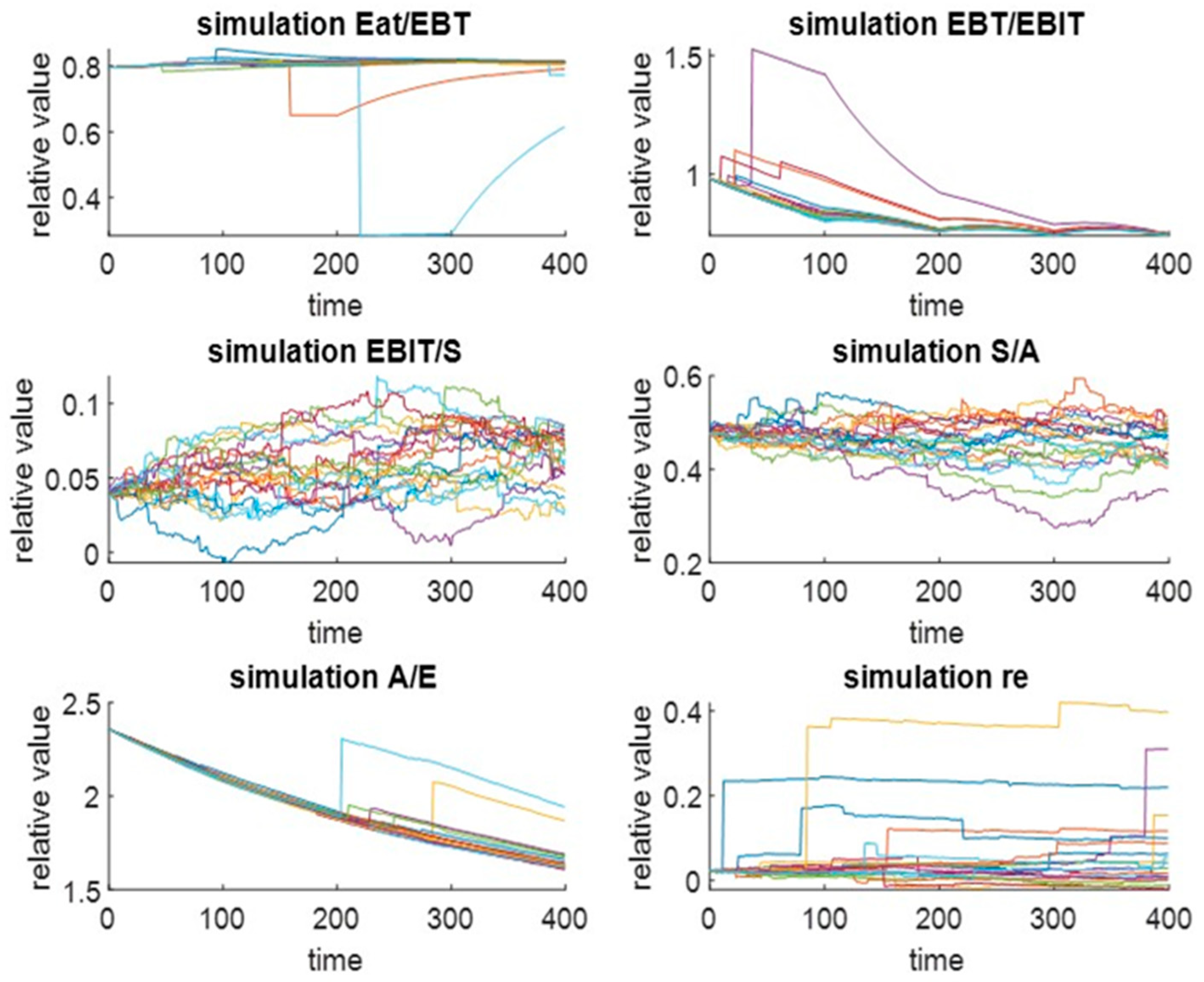
reflecting the t-copula function were utilised to generate random numbers and simulations. A presentation of 20 scenarios (colored), including their interdependencies, is shown in Figure 1, where asymmetry, fat tails, and jumps are apparent and verified. Likewise, every ratio demonstrates a different and unique distribution shape. Furthermore, the distribution of the relative EVA measure for one replication is illustrated in Figure 2 with decreasing distribution quantiles and negative asymmetry.
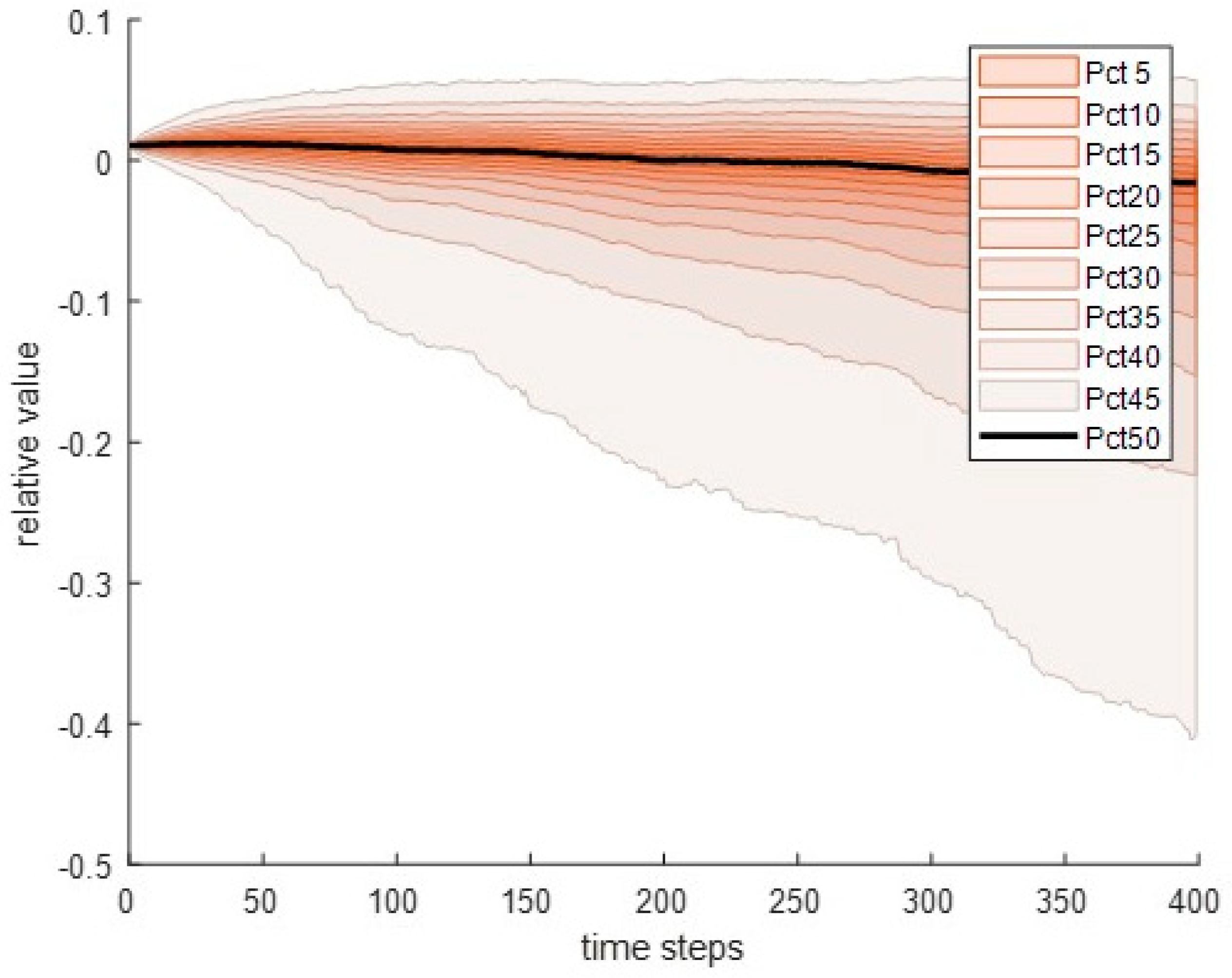
Step (vi) consists of the replication of step (v) 110 times due to the relative confidence interval of a standard error being less than 0.1. The results are shown in Table 6 for the mean value and quantiles, including the standard error and the parameter of preciseness. The predicted probability distribution development is presented in Figure 3.
Apparently, the precision of distribution parameters is commonly less than 10% and mostly less than 5%.

3.3. The Prediction Results of Relative Direct EVA Performance Measure by Simulation

The direct approach is simplified by comparing the decomposition approach (Section 3.1) in forecasting using only one measure and not using interdependencies. In step (i), the skew-t regression is realised for the direct relative EVA measure for the LDAMR and LDSMR models. The best model selected according to the AIC and the BIC is the LADMR model (see Table 7). Moreover, parameter α shows the right skewness of the direct relative EVA distribution, and parameter d f confirms the existence of fat tails. The value of parameter ω demonstrates a smaller scale.
In step (ii), the parameters of the NIG distribution residuals of the direct relative EVA are estimated by the method of moments, as in, e.g., [32], applying the Matlab n i g p a r function (see Table 4). The estimated parameters indicate lower heaviness α , high skewness β , a location close to zero μ , and a small scale δ .
The last step (iii) involves a simulation of the direct relative EVA measure using 400 steps in one scenario for a year with 105 scenarios. The Matlab function c o p u l a r n d 
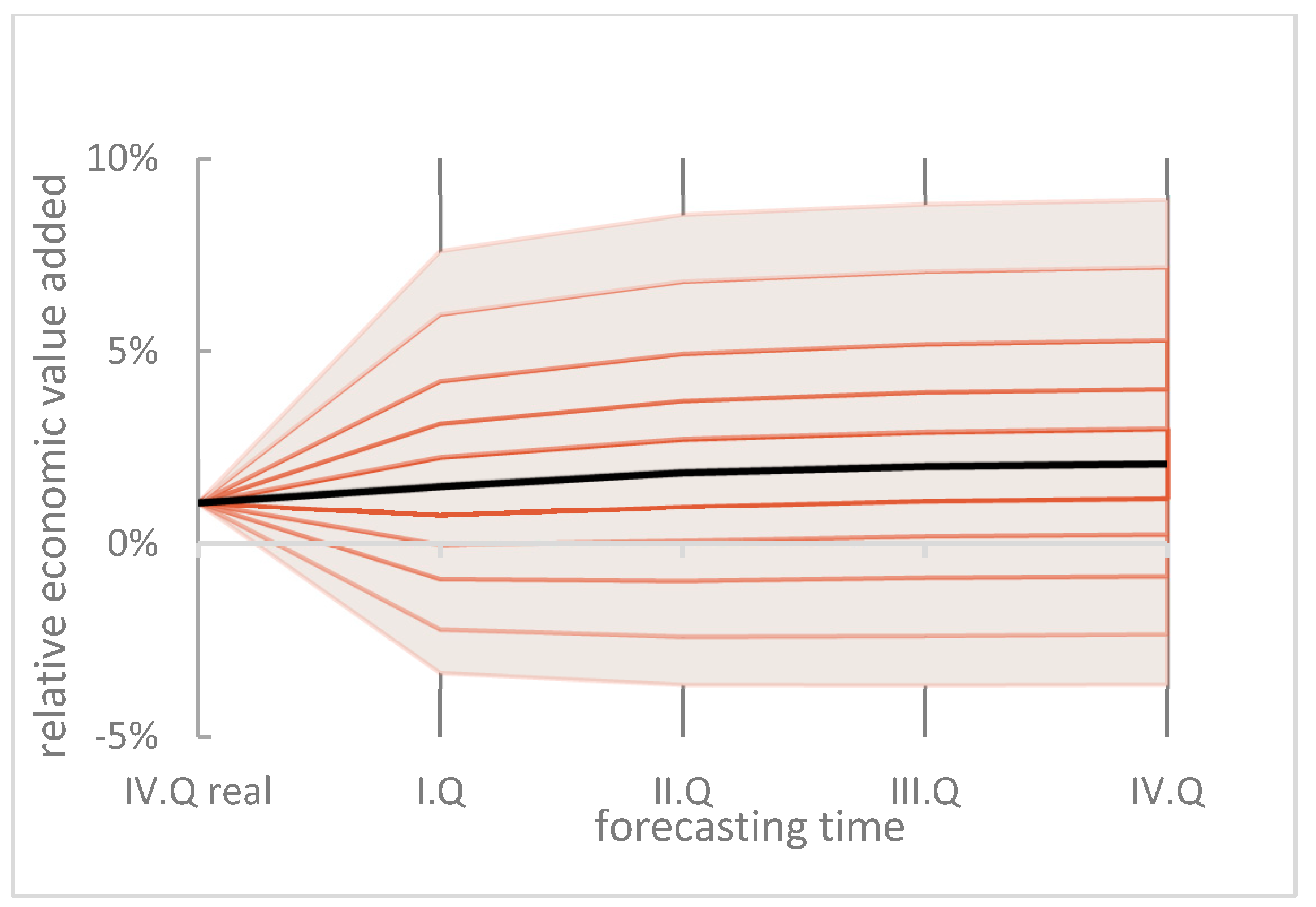
is used to generate random numbers and simulations. In step (iv), step (iii) is replicated ten times, and the distribution of the direct relative EVA is obtained due to the relative confidence interval of a standard error being determined to be less than 0.1 (see the results in Table 8 and Figure 4). The precision of the distribution in all parameters is less than 5%.

3.4. The Evaluation of Predictive Precision of EVAr Distribution Forecasts

The precision evaluation is focused on a one-quarter prediction. Firstly, quarterly predicted distributions for particular months are estimated using a simulation procedure stemming from the estimated models’ parameters. The parameters of the decomposed EVA are presented in Table 3, Table 4 and Table 5 and those for the direct EVA in Table 4 and Table 7. One simulation represents 106 scenarios, and 80 replications are applied. The resulting distribution quantiles, including relative precision, are show in Table 9 and Table 10.
The precision of the forecasted distribution was verified by the absolute and relative tests comparing the decomposed and direct EVA predicted distribution. The STATA esftest test, as in [68], was applied for the absolute test. For decomposed EVA, the W2 statistic is 2.492, with a significance of 0.6461, and for direct EVA, the W2 statistic is 2.669, with a significance of 0.61459. The H0 hypothesis was confirmed in both cases. Lower values affirm that the decomposed EVA coincides more with a uniform distribution and is more suitable. The relative test is evaluated using the logarithmic scoring rule, and STATA paired t-test. The score of the decomposed EVA is −1.9788, and the score of the direct EVA is −2.0718 (see Table 11). So, a bigger value means that the decomposed EVA forecasts the probability distribution better. The value of the STATA paired t-statistic is 2.5099, with a significance of 0.029. Therefore, hypothesis H0 is not confirmed, and the estimated forecasting models of EVA differ. Consequently, the decomposed model, when compared, is better as well.

4. Discussion and Conclusions

The relative EVA (Section 3.1) shows that the mean value decreases and so does the median. The quarterly forecast decreased from a starting value of 1.0605% for the mean value to −7.570%, and the median value decreased to −1.875%. The median looks more stable compared to the expected value, even with the same negative trend. The characteristics are huge and include negatively skewed quantile intervals. This is caused, among other things, by considering the interdependencies of ratios under the asymmetry of financial ratios and jumps. This phenomenon is hidden in relations among decomposed financial ratios.
The results of direct relative EVA distribution prediction (Section 3.2) show and confirm the historical behaviour of the measure. The median slightly increases to 2.086%, and the mean value is 2.307%. Quantiles are almost symmetrically distributed, with positive skewness. This approach does not include the possibility of using the hidden relations of the system behaviour in the prediction.
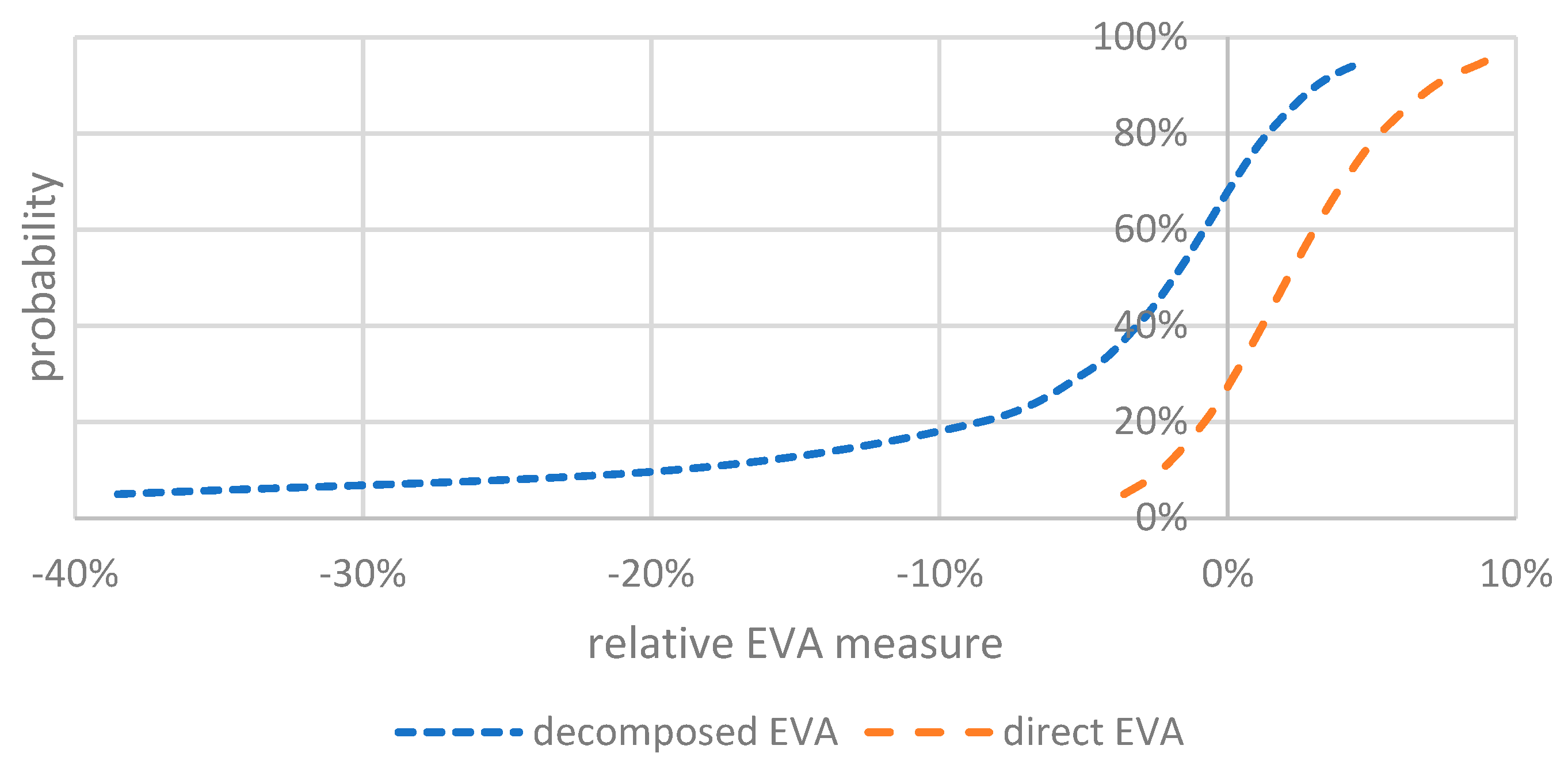
A comparison of the predicted distributions is apparent in Table 6 and Table 7, and a graphical comparison for the fourth quarter is demonstrated in Figure 5.
The comparison of the decomposed and direct relative EVA one-quarter prediction (Section 3.3) was tested using absolute and relative tests. The absolute test showed that the distribution prediction for the decomposed EVA is more accurate in comparison with the direct EVA. Similarly, the relative scoring logarithm test and the paired t-statistic confirmed the better accuracy of the decomposed EVA. Both applied tests verified the superiority of the decomposed EVA forecast model in the particular data case.
The proposed and applied probability distribution decomposition forecasting method is a more adequate and precise approach allowing the prediction of complete uncertainty compared to point prediction.
The proposed innovative advanced forecasting simulation method was verified as a proper conception for the problem of modelling and reflecting empirical data. The LDAMR and LDSMR processes sufficiently fit the chosen financial ratios, and the skew t-regression estimation was valid. The Monte-Carlo simulation of the NIG distribution with a t-copula adequately serves for a decomposed relative EVA distribution prediction, including its precision. It was shown that the direct relative EVA distribution prediction captures the historical behaviour of the complex measure only superficially and simplistically. Therefore, the direct EVA approach is unsuitable for predicting complex, synthetic, and risk measures, such as an EVA indicator. The EVA measure can be explained by reflecting the complexity and comprehensiveness of particular indicators, including their relationship phenomena hidden in financial performance.
The empirical results were verified, proving that the mean value and median of the decomposed relative EVA of the Czech automotive production sector tends to decrease in the future, with negative asymmetry and high volatility hidden in the decomposition of the financial ratios. The median is more stable in comparison to the mean value, even with a negative trend. The applied model led to huge volatility, with extreme values. This volatility is caused, among other things, by considering the ratios’ interdependencies and jumps. This phenomenon is hidden in the empirical historical data and in the relations among exact pyramid-decomposed financial ratios, and it looks both realistic and interesting.
The prediction of the decomposed relative EVA confirms that the sector is exposed to some fundamental structural changes. It is influenced by the limited qualified workers’ capacity, the efficiency of production, and industry competition. The sector is also affected by economic shocks caused by regulatory ecological measures, competitiveness, and substantial technological changes. New phenomena not considered in the model are pandemics, military attacks, and the shortage of spare parts and input material sources.
Further research can be devoted to developing other pyramid decomposition, Levy model types, copula functions, parameter estimations, and simulation approaches. Time series can be prolonged, and crisis periods can be included in them. For comparison, the financial performance of other sectors can also be analysed and predicted.

Author Contributions

Conceptualisation: Z.Z. and D.D.; Methodology: Z.Z. and D.D.; Data Curation: I.R. and A.P.; Software: Z.Z.; Writing—Original Draft: Z.Z.; Writing—Review and Editing: D.D., K.L., A.P. and I.R.; Funding acquisition: D.D.; Formal analysis and investigation: Z.Z., D.D., K.L., A.P. and I.R. All authors have read and agreed to the published version of the manuscript.

Funding

The paper is supported by the Grant Agency of the VSB-Technical University Ostrava SP2022/58, SP2023/008.

Data Availability Statement

Not applicable here.

Acknowledgments

The paper is supported by the Grant Agency of the VSB-Technical University Ostrava SP2022/58, SP2023/008. This support is gratefully acknowledged.

Conflicts of Interest

The authors declare no conflict of interest.

References

  1. Tay, A.S.; Wallis, K.F. Density forecasting: A survey. J. Forecast. 2000, 19, 235–254. [Google Scholar] [CrossRef]
  2. Cho, S.Y.; Lee, C. Managerial Efficiency, Corporate Social Performance, and Corporate Financial Performance. J. Bus. Ethics 2017, 158, 467–486. [Google Scholar] [CrossRef]
  3. Park, B.J. Corporate social and financial performance: The role of the firm life cycle in business groups. Sustainability 2021, 13, 7445. [Google Scholar] [CrossRef]
  4. Alshehhi, A.; Nobanee, H.; Khare, N. The impact of sustainability practices on corporate financial performance: Literature trends and future research potential. Sustainability 2018, 10, 494. [Google Scholar] [CrossRef] [Green Version]
  5. Athanassakos, G. Value-based management, EVA and stock price performance in Canada. Manag. Decis. 2009, 45, 1397–1411. [Google Scholar] [CrossRef]
  6. Dluhošová, D. An analysis of financial performance using the EVA method. Czech J. Econ. Financ. (Financ. Uver) 2004, 54, 541–559. Available online: https://journal.fsv.cuni.cz/storage/996_04_541-559.pdf (accessed on 22 March 2023).
  7. Woodhouse, K.; Mather, P.; Ranasinghe, D. Externally reported performance measures and benchmarks in Australia. Account. Financ. 2017, 57, 879–905. [Google Scholar] [CrossRef]
  8. Borodin, A.; Mityushina, I.; Streltsova, E.; Kulikov, A.; Yakovenko, I.; Namitulina, A. Mathematical Modeling for Financial Analysis of an Enterprise: Motivating of Not Open Innovation. J. Open Innov. Technol. Mark. Complex 2021, 7, 79. [Google Scholar] [CrossRef]
  9. Jencova, S.; Litavcova, E.; Vasanicova, P. Implementation of Du Pont Model in Non-Financial Corporations. Montenegrin J. Econ. 2018, 14, 131–141. [Google Scholar] [CrossRef]
  10. Jeppson, N.H.; Ruddy, J.A.; Salerno, D.F. The influence of social media usage on the DuPont method of analysis. J. Corp. Account. Financ. 2021, 32, 31–44. [Google Scholar] [CrossRef]
  11. Kryzanowski, L.; Mohsni, S. Earnings forecasts and idiosyncratic volatilities. Int. Rev. Financ. Anal. 2015, 41, 107–123. [Google Scholar] [CrossRef]
  12. Jin, Y. DuPont Analysis, Earnings Persistence, and Return on Equity: Evidence from Mandatory IFRS Adoption in Canada. Account. Perspect. 2017, 16, 205–235. [Google Scholar] [CrossRef]
  13. Zmeškal, Z.; Dluhošová, D. Company financial performance prediction on economic value added measure by simulation methodology. In Proceedings of the 27th International Conference on Mathematical Methods in Economics, Mathematical Methods in Economics, Prague, Czech Republic, 9–11 September 2009; pp. 352–358. [Google Scholar]
  14. Addoum, J.M.; Delikouras, S.; Korniotis, G.M.; Kumar, A. Income Hedging, Dynamic Style Preferences, and Return Predictability. J. Financ. 2014, 74, 2055–2106. [Google Scholar] [CrossRef]
  15. Alti, A.; Titman, S. A Dynamic Model of Characteristic-Based Return Predictability. J. Financ. 2019, 74, 3187–3216. [Google Scholar] [CrossRef]
  16. Burgstahler, D.; Eames, M. Management of Earnings and Analysts’ Forecasts to Achieve Zero and Small Positive Earnings Surprises. J. Bus. Financ. Account. 2006, 33, 633–652. [Google Scholar] [CrossRef]
  17. Chang, V.; Ramachandran, M. Financial Modeling and Prediction as a Service. J. Grid Comput. 2017, 15, 177–195. [Google Scholar] [CrossRef] [Green Version]
  18. Chiang, C.; Dai, W.; Fan, J.; Hong, H.; Tu, J. Robust Measures of Earnings Surprises. J. Financ. 2019, 74, 943–983. [Google Scholar] [CrossRef]
  19. Yohn, T.L. Research on the use of financial statement information for forecasting profitability. Account. Financ. 2020, 60, 3163–3181. [Google Scholar] [CrossRef]
  20. Marček, D. Forecasting of financial data: A novel fuzzy logic neural network based on error-correction concept and statistics. Complex Intell. Syst. 2018, 4, 95–104. [Google Scholar] [CrossRef] [Green Version]
  21. Marček, D. Some Statistical and CI Models to Predict Chaotic High-frequency Financial Data. J. Intell. Fuzzy Syst. 2020, 39, 6419–6430. [Google Scholar] [CrossRef]
  22. Oktoviany, P.; Knobloch, R.; Korn, R. A machine learning-based price state prediction model for agricultural commodities using external factors. Decis. Econ. Financ. 2021, 44, 1063–1085. [Google Scholar] [CrossRef]
  23. Swanson, N.R.; Urbach, R. Prediction and simulation using simple models characterised by nonstationarity and seasonality. Int. Rev. Econ. Financ. 2015, 40, 312–323. [Google Scholar] [CrossRef] [Green Version]
  24. Byun, K.; Song, S. Value at Risk of portfolios using copulas. Commun. Stat. Appl. Methods 2021, 28, 59–79. [Google Scholar] [CrossRef]
  25. Choroś-Tomczyk, B.; Härdle, W.K.; Overbeck, L. Copula dynamics in CDOs. Quant. Financ. 2014, 14, 1573–1585. [Google Scholar] [CrossRef]
  26. Pircalabu, A.; Benth, F.E. A regime-switching copula approach to modeling day-ahead prices in coupled electricity markets. Energy Econ. 2017, 68, 283–302. [Google Scholar] [CrossRef] [Green Version]
  27. Sabino, P.; Petroni, N.C. Fast simulation of tempered stable Ornstein–Uhlenbeck processes. Comput Stat. 2022, 37, 2517–2551. [Google Scholar] [CrossRef]
  28. Taufer, E.; Leonenko, N. Simulation of Lévy-driven Ornstein–Uhlenbeck processes with given marginal distribution. Comput. Stat. Data Anal. 2009, 53, 2427–2437. [Google Scholar] [CrossRef]
  29. Barndorff-Nielsen, O.E. Normal inverse Gaussian distributions and stochastic volatility modelling. Scand. J. Stat. 1997, 24, 1–13. Available online: https://www.jstor.org/stable/4616433 (accessed on 5 March 2023). [CrossRef]
  30. Fragiadakis, K.; Karlis, D.; Meintanis, S.G. Tests of fit for normal inverse Gaussian distributions. Stat. Methodol. 2009, 6, 553–564. [Google Scholar] [CrossRef]
  31. Chevallier, J.; Goutte, S. Estimation of Lévy-driven Ornstein–Uhlenbeck processes: Application to modeling of CO2 and fuel-switching. Ann. Oper. Res. 2017, 255, 169–197. [Google Scholar] [CrossRef]
  32. Karlis, D. An EM Type Algorithm for Maximum Likelihood Estimation of the Normal-Inverse Gaussian Distribution. Stat. Probab. Lett. 2002, 57, 43–52. [Google Scholar] [CrossRef]
  33. Mejía Vega, C.A. Calibration of the exponential Ornstein–Uhlenbeck process when spot prices are visible through the maximum log-likelihood method. Example with gold prices. Adv. Differ. Equ. 2018, 269. [Google Scholar] [CrossRef]
  34. Aguilar, J.P. Explicit option valuation in the exponential NIG model. Quant. Financ. 2021, 21, 1281–1299. [Google Scholar] [CrossRef]
  35. Godin, F.; Mayoral, S.; Morales, M. Contingent Claim Pricing Using a Normal Inverse Gaussian Probability Distortion Operator. J. Risk Insur. 2012, 79, 841–886. [Google Scholar] [CrossRef]
  36. Lahcene, B. On Extended Normal Inverse Gaussian Distribution: Theory, Methodology, Properties and Applications. Am. J. Appl. Math. Stat. 2009, 7, 224–230. [Google Scholar] [CrossRef]
  37. Rydberg, T.H. The normal inverse Gaussian Levy process: Simulation and approximation. Comm. Statist. Stoch. Model. 1997, 13, 887–910. [Google Scholar] [CrossRef]
  38. Song, S.; Li, H. Predicting VaR for China’s stock market: A score-driven model based on normal inverse Gaussian distribution. Int. Rev. Financ. Anal. 2022, 82, 102180. [Google Scholar] [CrossRef]
  39. Barndorff-Nielsen, O.E.; Shephard, N. Non-Gaussian Ornstein-Uhlenbeck-based models and some of their uses in financial economics. J. R. Stat. Soc. Ser. B (Stat. Methodol.) 2001, 63, 167–241. [Google Scholar] [CrossRef]
  40. Abdelrazeq, I.; Ivanoff, B.G.; Kulik, R.F. Model verification for Levy-driven Ornstein-Uhlenbeck processes. Electron. J. Stat. 2014, 8, 1029–1062. [Google Scholar] [CrossRef]
  41. Benth, F.E.; Di Persio, L.; Lavagnini, S. Stochastic Modeling of Wind Derivatives in Energy Markets. Risks 2018, 6, 56. [Google Scholar] [CrossRef] [Green Version]
  42. Benth, F.E.; Pircalabu, A. A non-Gaussian Ornstein–Uhlenbeck model for pricing wind power futures. Appl. Math. Financ. 2018, 25, 36–65. [Google Scholar] [CrossRef] [Green Version]
  43. Benth, F.E.; Šaltyté-Benth, J. The normal inverse Gaussian distribution and spot price modelling in energy markets. Int. J. Theor. Appl. Financ. 2004, 7, 177–192. [Google Scholar] [CrossRef]
  44. Brix, A.F.; Lunde, A.; Wei, W. A generalised Schwartz model for energy spot prices—Estimation using a particle MCMC method. Energy Econ. 2018, 72, 560–582. [Google Scholar] [CrossRef] [Green Version]
  45. Deschatre, T.; Féron, O.; Gruet, P. A survey of electricity spot and futures price models for risk management applications. Energy Econ. 2021, 102, 105504. [Google Scholar] [CrossRef]
  46. Endres, S.; Stübinger, J. Optimal trading strategies for Lévy-driven Ornstein–Uhlenbeck processes. Appl. Econ. 2019, 51, 3153–3169. [Google Scholar] [CrossRef]
  47. Bao, Y.; Lee, T.-H.; Saltoğlu, B. Comparing density forecast models. J. Forecast. 2007, 26, 203–225. [Google Scholar] [CrossRef] [Green Version]
  48. Bauwens, L.; Giot, P.; Grammig, J.; Veredas, D. A comparison of financial duration models via density forecasts. Int. J. Forecast. 2004, 20, 589–609. [Google Scholar] [CrossRef]
  49. Crisóstomo, R.; Couso, L. Financial density forecasts: A comprehensive comparison of risk-neutral and historical schemes. J. Forecast. 2018, 37, 589–603. [Google Scholar] [CrossRef] [Green Version]
  50. Egorov, A.V.; Hong, Y.; Li, H. Validating forecasts of the joint probability density of bond yields: Can affine models beat random walk? J. Econom. 2006, 135, 255–284. [Google Scholar] [CrossRef]
  51. Hyndman, R.J.; Fan, S. Density Forecasting for Long-Term Peak Electricity Demand. IEEE Trans. Power Syst. 2010, 25, 1142–1153. [Google Scholar] [CrossRef] [Green Version]
  52. Rossi, B.; Sekhposyan, T. Conditional predictive density evaluation in the presence of instabilities. J. Econom. 2013, 177, 199–212. [Google Scholar] [CrossRef] [Green Version]
  53. Barhoumi, K.; Darné, O.; Ferrara, L. Are disaggregate data useful for factor analysis in forecasting French GDP? J. Forecast. 2010, 29, 132–144. [Google Scholar] [CrossRef] [Green Version]
  54. Cortazar, G.; Naranjo, L. An N-factor Gaussian model of oil futures prices. J. Futures Mark. 2006, 26, 243–268. [Google Scholar] [CrossRef]
  55. Kim, K.H. Density forecasting through disaggregation. Int. J. Forecast. 2011, 27, 394–412. [Google Scholar] [CrossRef]
  56. Harding, B.; Tremblay, C.; Cousineau, D. Standard errors: A review and evaluation of standard error estimators using Monte Carlo simulations. Quant. Methods Psychol. 2014, 10, 107–123. [Google Scholar] [CrossRef]
  57. Hoad, K.; Robinson, S.; Davies, R. Automated selection of the number of replications for a discrete-event simulation. J. Oper. Res. Soc. 2010, 61, 1632–1644. Available online: http://www.jstor.org/stable/40926090 (accessed on 15 March 2023). [CrossRef]
  58. Koehler, E.; Brown, E.; Haneuse, S.J. On the Assessment of Monte Carlo Error in Simulation-Based Statistical Analyses. Am. Stat. 2009, 63, 155–162. [Google Scholar] [CrossRef] [Green Version]
  59. Nakayama, M.K. Confidence Intervals for Quantiles Using Sectioning When Applying Variance-Reduction Techniques. ACM Trans. Model. Comput. Simul. 2014, 24, 1–21. [Google Scholar] [CrossRef]
  60. Diebold, F.X.; Gunther, T.A.; Tay, A.S. Evaluating Density Forecasts with Applications to Financial Risk Management. Int. Econ. Rev. 1998, 39, 863–883. [Google Scholar] [CrossRef] [Green Version]
  61. Diebold, F.X.; Mariano, R.S. Comparing Predictive Accuracy. J. Bus. Econ. Stat. 2002, 20, 134–144. [Google Scholar] [CrossRef]
  62. Amisano, G.; Giacomini, R. Comparing Density Forecasts via Weighted Likelihood Ratio Tests. J. Bus. Econ. Stat. 2007, 25, 177–190. [Google Scholar] [CrossRef]
  63. Cees, D.; Panchenko, V.; van Dijk, D. Likelihood-Based Scoring Rules for Comparing Density Forecasts in Tails. Econometrics 2011, 163, 215–230. [Google Scholar] [CrossRef] [Green Version]
  64. Corradi, V.; Swanson, N.R. Predictive density and conditional confidence interval accuracy tests. J. Econom. 2006, 135, 187–228. [Google Scholar] [CrossRef]
  65. Mitchell, J.; Hall, S.G. Evaluating, Comparing and Combining Density Forecasts Using the KLIC with an Application to the Bank of England and NIESR ‘Fan’ Charts of Inflation. Oxf. Bull. Econ. Stat. 2005, 67, 995–1033. [Google Scholar] [CrossRef]
  66. Lavagnini, S. CARMA Approximations and Estimation. Front. Appl. Math. Stat. 2020, 6, 37. [Google Scholar] [CrossRef]
  67. Marchenko, Y.V.; Genton, M.G. A suite of commands for fitting the skew-normal and skew-t models. Stata J. 2010, 10, 507–539. [Google Scholar] [CrossRef] [Green Version]
  68. Sebastian, J. Goerg Johannes Kaiser Nonparametric testing of distributions—The Epps–Singleton two-sample test using the empirical characteristic function. Stata J. 2009, 9, 454–465. [Google Scholar]
  69. FASPMO Finanční Analýza Podnikové Sféry MPO (2007–2019). Available online: https://www.mpo.cz/cz/rozcestnik/analyticke-materialy-a-statistiky/analyticke-materialy (accessed on 14 January 2023).
Figure 1. Scenario simulations (colored) of the investigated financial ratios.
Forecasting 05 00025 g001
Figure 2. Relative EVA quantiles predicted distribution with the t-copula (one replication).
Forecasting 05 00025 g002
Figure 3. The relative EVA quantiles predicted distribution with the t-copula (110 replications).
Forecasting 05 00025 g003
Figure 4. The direct relative EVA quantiles predicted distribution (10 replications).
Forecasting 05 00025 g004
Figure 5. A comparison of decomposed and direct relative EVA predicted distribution for the 4th quarter.
Forecasting 05 00025 g005
Table 1. Input quarter financial ratios data obtained quarterly, 1Q 2007–4Q 2019 (in the sample).
QuarterEat/EBTEBT/EBITEBIT/SS/AA/EreEVAr
10.750140.950040.078810.474911.982570.026580.02630
20.750860.948670.078070.907832.029030.025380.07706
30.740610.943540.073961.301601.948370.026600.10446
40.743660.940230.073271.781991.922890.025660.14988
50.777340.944130.077940.445401.988270.023690.02697
60.775770.945860.085510.864502.007490.025510.08337
70.768790.937050.077591.278751.973740.026290.11477
80.754280.918630.067321.600541.983940.026170.12195
93.18631−0.165990.016250.327932.163580.03535−0.04145
100.815361.363200.054310.381172.127250.038160.01078
110.781561.087120.028510.357162.074870.03816−0.02021
120.512250.978500.010800.404052.146070.03894−0.03425
130.789971.101920.061970.417532.172260.037470.01146
140.797200.904600.085970.432992.177780.032310.02615
150.780661.293190.035560.362512.148570.03062−0.00266
160.779581.182830.012400.420342.244650.03080−0.02002
170.795401.071710.058440.435282.380180.031970.01964
180.810161.009980.065420.440842.297020.030860.02334
190.802541.593660.045240.384162.269780.031270.01918
200.788950.517200.037920.428812.417410.03023−0.01419
210.799851.045400.067000.441842.452630.033890.02682
220.794810.826260.059990.420842.407680.029180.01074
230.793391.037880.041330.361012.255900.02895−0.00123
240.791750.988470.026530.405372.264100.02850−0.00944
250.783580.906140.051870.418122.184590.024360.00928
260.789030.836800.054640.434422.129700.027630.00574
270.803331.006090.057030.405542.095790.023030.01615
280.784110.977000.033920.440272.130280.02721−0.00284
290.799930.873240.066100.466462.226860.023400.02456
300.804830.920380.069170.470992.149620.023950.02793
310.798590.833850.065750.433222.182570.022290.01911
320.807970.840790.051760.447782.236240.020450.01476
330.803490.970890.112680.469542.380480.019470.07878
340.806610.978000.070620.466762.282470.019930.03942
350.805060.958610.062890.428882.168270.019700.02543
360.803780.983880.049720.473142.099240.019620.01943
370.805390.866070.074050.470492.231600.019660.03457
380.810840.926450.082470.510322.172260.018460.05022
390.806211.027780.071860.416652.130810.018010.03485
400.818980.881900.064250.552752.065320.017350.03562
410.802300.961620.074720.521252.227590.017890.04905
420.802730.925730.079950.414212.088790.017570.03383
430.799290.921120.043660.488332.075910.017600.01499
440.804080.995360.057800.461642.231600.019400.02826
450.797450.970590.061320.483622.375380.023290.03123
460.803910.957800.069890.502162.334030.023790.03928
470.766340.903020.038220.414582.314490.023790.00158
480.798520.929800.030400.513442.240470.023530.00243
490.792140.973200.061310.477492.550760.023430.03414
500.803210.978330.052110.515242.454040.023940.02785
510.791900.953080.042750.457202.414470.023940.01168
520.795480.982830.038680.477192.358710.023430.01061
Table 2. Input quarter financial ratios data obtained monthly (out of sample).
MonthEat/EBTEBT/EBITEBIT/SS/AA/EreEVAr
BeginningEnding
1/20202/20190.795480.982830.038680.477192.358710.023430.01061
2/20201/20200.706670.857870.039110.466442.420990.024630.00214
3/20202/20200.738080.940200.035680.599352.376400.03882−0.00355
4/20203/20200.785190.805880.041630.477012.319120.025930.00321
5/20204/20200.613530.592150.021470.724702.380580.03733−0.02387
6/20205/20200.581240.631630.020130.770642.366440.05973−0.04625
7/20206/20200.645820.557320.022810.768292.338670.03394−0.01918
8/20207/20200.692660.703020.027970.739582.425580.02986−0.00543
9/20208/20200.685370.743580.026440.920022.389210.03898−0.00936
10/20209/20200.729120.675980.029091.220802.303920.031440.00889
11/202010/20200.582270.784970.033771.200682.669360.036990.01248
12/202011/20200.718380.830680.031911.406942.573660.048670.02029
1/202112/20200.632740.925680.029090.845072.249240.023320.00907
2/20211/20210.718380.942090.031651.312222.453150.042270.02669
3/20212/20210.534470.905990.039540.642222.426090.024070.00576
Table 3. Estimated parameters of LDAMR and LDSMR models.
VariableEat/EBTEBT/EBITEBIT/S
ModelLDSMRLDAMRLDSMRLDAMRLDSMRLDAMR
Ln(x)−0.541 *** −0.581 *** −1.069 ***
x −0.995 *** −1.338 *** −0.728 ***
constant−0.114 ***0.801 ***−0.029 ***1.258 ***−2.803 ***0.059 ***
alpha−1.050−1.9650.0170.313−0.607−2.164
omega0.009180.008150.029600.048460.278320.02047
df0.898530.908460.847051.291751.590423.81904
LL112.021126.31539.12239.687−38.228130.651
chi218,000250,00084.363257.75240.38066.421
p000000
BIC−204.38−232.97−58.68−59.7296.12−241.64
AIC−214.04−242.63−68.24−69.3786.46−251.30
a 0.9945541 1.3379895 0.7281569
b 0.8056467 0.9401605 0.0811942
VariableS/AA/Ere
ModelLDSMRLDAMRLDSMRLDAMRLDSMRLDAMR
Ln(x)−0.567 *** −0.181 ** −0.028
x0−0.474 *** −0.209 ** −0.037
constant−0.436 ***0.216 ***0.0990.364 **−0.1220.001
alpha−0.267−0.0174.8264.6210.3210.204
omega0.067340.034530.058780.126190.046280.00109
df3.493846.9240417.6370214.069372.011741.71258
LL42.82777.31097.03357.20958.271243.776
chi223.47113.0117.87410.5150.5510.894
p000.0050.0010.4580.345
BIC−66.85−135.81−174.41−94.76−96.88−467.89
AIC−75.65−144.62−184.07−104.42−106.54−477.55
a 0.47494630.1808063 0.0367403
b 0.45384350.5453796 0.0146380
Legend: ** and *** denote significance at 5% and 1%, respectively.
Table 4. NIG residuals distribution parameters of the chosen ratio models.
Model Ratios αβμδ
Eat/EBTLDAMR11.1−10.2670.00840.001
EBT/EBITLDAMR202.3201.861−0.14470.0057
EBIT/SLDAMR104.615.0765−0.01470.0426
S/ALDAMR64.596114.1858−0.02290.1003
A/ELDSMR105.2104.37−0.06940.0062
reLDAMR12.912.3956−0.00020.0087
EVA directLDAMR51.397614.7134−0.00340.0518
Table 5. The correlation matrix of the residuals.
REat/EBTEBT/EBITEBIT/SS/AA/Ere
Eat/EBT1−0.24350.6426−0.0029−0.8151−0.4035
EBT/EBIT−0.24351−0.1462−0.17720.21150.3274
EBIT/S0.6426−0.146210.217−0.6158−0.3574
S/A−0.0029−0.17720.2171−0.00780.1567
A/E−0.81510.2115−0.6158−0.007810.4517
re−0.40350.3274−0.35740.15670.45171
Table 6. Quarterly prediction results of relative EVA measure in %.
QuarterI. QII. Q
Parameter E r S E r d r E r S E r d r
M e a n −0.8980.2319.578−2.7870.1782.376
M e d i a n ( · ) 0.4680.0560.897−0.0620.0607.271
Quantiles (%)954.4020.0280.0054.8330.0360.006
903.3000.0300.0183.5080.0360.020
802.2080.0350.0672.1730.0410.078
701.5270.0410.1581.3130.0450.205
600.9700.0480.3470.6060.0510.597
500.4680.0560.897−0.0620.0607.271
40−0.0530.0699.066−0.7700.0730.673
30−0.6430.0880.813−1.6450.0990.358
20−1.4850.1280.358−3.0470.1620.222
10−3.5700.2840.156−7.1430.4050.111
5−8.2930.7400.075−16.2350.8260.043
QuarterIII. QIV. Q
Parameter E r S E r d r E r S E r d r
M e a n −5.8030.1741.119−7.5700.3981.960
M e d i a n ( · ) −1.1220.0730.486−1.8750.1720.681
Quantiles (%)954.6700.0450.0084.6880.1030.018
903.1920.0460.0283.0800.1040.066
801.6580.0490.1231.3820.1130.341
700.6330.0550.5140.2120.1263.532
60−0.2470.0621.779−0.8120.1441.254
50−1.1220.0730.486−1.8750.1720.681
40−2.1250.0930.307−3.1450.2180.490
30−3.5220.1290.217−5.0080.3060.362
20−6.1370.2130.145−8.5820.4960.241
10−14.4250.4430.060−19.3320.9940.101
5−30.3950.7570.021−38.5081.6490.036
Table 7. The estimated parameters of LDAMR and LDSMR models for direct EVA.
ModelLDSMRLDAMR
VariableEVAEVA
Ln(x)−0.1950
x0−0.706 ***
constant−1.072 *0.007
alpha0.6040.537
omega0.620020.02032
df1.544962.28416
LL−65.996105.743
chi214.66314.663
p00
BIC150.68−191.83
AIC141.99−201.49
a 0.7060
b 0
Legend: * and *** denote significance at 10% and 1%, respectively.
Table 8. Quarterly prediction results of direct relative EVA measure in %.
QuarterI. QII. Q
Parameter E r S E r d r E r S E r d r
M e a n 1.7270.0030.2532.0570.0030.187
M e d i a n ( · ) 1.4950.0020.0411.8370.0050.084
Quantiles (%)957.6240.0100.0048.5210.0090.003
905.9760.0070.0086.8060.0060.006
804.2420.0040.0134.9380.0030.008
703.1360.0030.0233.7110.0010.008
602.2630.0020.0262.7210.0040.036
501.4950.0020.0411.8370.0050.084
400.7530.0020.0840.9780.0030.086
30−0.0230.0043.9360.0820.0010.352
20−0.9190.0050.079−0.9670.0040.059
10−2.2010.0050.016−2.4220.0040.012
5−3.3270.0100.009−3.6590.0050.004
QuarterIII. QIV. Q
Parameter E r S E r d r E r S E r d r
M e a n 2.2250.0020.1232.3070.0040.264
M e d i a n ( · ) 2.0000.0060.0812.0860.0050.066
Quantiles (%)958.8260.0080.0038.9120.0090.003
907.0780.0070.0077.1830.0050.005
805.1730.0020.0055.2760.0040.012
703.9240.0020.0114.0260.0060.035
602.9120.0040.0363.0080.0070.059
502.0000.0060.0812.0860.0050.066
401.1190.0060.1351.1920.0050.109
300.1910.0060.7470.2580.0050.456
20−0.8790.0070.120−0.8160.0030.060
10−2.3730.0040.011−2.3230.0060.020
5−3.6450.0090.007−3.5990.0070.006
Table 9. Monthly quarter prediction results of decomposed relative EVA measure in %.
Month3/20204/20205/20206/2020
Parameter E r d r E r d r E r d r E r d r
Er (Q)−0.8989.578−2.2161.192−2.7991.665−2.2851.126
Medr (Q)0.4680.897−0.0847.266−0.8901.978−0.1513.743
Quantiles (%)954.4020.0053.8070.3573.3520.6933.7300.333
903.3000.0182.7340.3902.2010.8402.6590.366
802.2080.0671.6700.5361.0381.5351.5970.511
701.5270.1580.9900.8700.2895.3740.9200.855
600.9700.3470.4352.036−0.3225.0200.3662.219
500.4680.897−0.0847.266−0.8901.978−0.1513.743
40−0.0539.066−0.6271.763−1.4791.373−0.6931.496
30−0.6430.813−1.2781.089−2.1681.173−1.3430.986
20−1.4850.358−2.2580.922−3.1651.184−2.3220.869
10−3.5700.156−5.0031.071−5.7161.610−5.0671.046
5−8.2930.075−11.6051.456−11.7792.459−11.6761.443
Month7/20208/20209/202010/2020
Parameter E r d r E r d r E r d r E r d r
Er (Q)−3.3011.533−5.3920.888−2.8361.795−2.1201.959
Medr (Q)−1.3700.862−3.4670.329−0.9101.332−0.1298.026
Quantiles (%)952.7310.8670.7123.3113.2540.7684.2420.527
901.6121.174−0.4234.4222.1220.9353.0660.575
800.4893.351−1.5671.0300.9821.7431.8710.804
70−0.2326.975−2.3040.6860.2496.7371.0971.324
60−0.8212.059−2.9060.565−0.3514.9630.4633.232
50−1.3700.862−3.4670.329−0.9101.332−0.1298.026
40−1.9411.111−4.0510.512−1.4911.478−0.7432.501
30−2.6131.042−4.7360.550−2.1741.273−1.4631.579
20−3.5941.126−5.7290.671−3.1651.291−2.5011.347
10−6.1591.641−8.2901.143−5.7261.761−5.1261.583
5−12.2632.600−14.3782.074−11.8172.687−11.3962.233
Month11/202012/20201/20212/2021
Parameter E r d r E r d r E r d r E r d r
Er (Q)−2.4771.479−0.7465.072−0.5757.322−0.5917.761
Medr (Q)−0.4961.8581.1830.9051.3010.9471.1781.180
Quantiles (%)954.3000.4486.5790.3726.9860.4187.6380.415
903.0330.5045.1770.3735.5150.4165.9850.419
801.7220.7653.7020.4393.9610.4824.2180.501
700.8661.4822.7310.5682.9350.6163.0450.663
600.1618.2491.9300.8162.0880.8742.0770.987
50−0.4961.8581.1830.9051.3010.9471.1781.180
40−1.1751.4180.4154.5650.4934.3930.2619.384
30−1.9651.058−0.4704.900−0.4326.047−0.7793.798
20−3.0800.983−1.6871.915−1.6932.151−2.1641.891
10−5.7251.232−4.3711.610−4.3901.774−4.9391.710
5−11.9561.841−10.4252.033−10.2902.245−10.5052.281
Table 10. Monthly quarter prediction results of direct relative EVA measure in %.
Month3/20204/20205/20206/2020
Parameter E r d r E r d r E r d r E r d r
Er (Q)1.7270.2531.3010.1711.0180.2191.3580.176
Medr (Q)1.4950.0411.0610.1570.7780.2141.1170.160
Quantiles (%)957.6240.0047.1460.2066.8630.2147.2030.143
905.9760.0085.5080.1725.2250.1815.5680.105
804.2420.0133.7880.1223.5050.1323.8450.160
703.1360.0232.6910.1182.4080.1322.7480.175
602.2630.0261.8240.1601.5410.1891.8820.185
501.4950.0411.0610.1570.7780.2141.1170.160
400.7530.0840.3280.6320.0454.5620.3870.834
30−0.0233.936−0.4400.478−0.7230.291−0.3841.054
20−0.9190.079−1.3350.269−1.6180.222−1.2760.316
10−2.2010.016−2.6090.217−2.8920.196−2.5500.190
5−3.3270.009−3.7370.216−4.0200.201−3.6740.197
Month7/20208/20209/202010/2020
Parameter E r d r E r d r E r d r E r d r
Er (Q)0.0129.801−1.1050.2020.2480.4660.9250.241
Medr (Q)−0.2270.461−1.3440.1240.0099.9760.6880.238
Quantiles (%)955.8670.2114.7400.3106.0940.1826.7680.181
904.2220.1293.1030.3064.4570.1195.1290.148
802.4980.1551.3820.3342.7330.1493.4100.131
701.4000.2530.2861.1111.6380.2112.3130.126
600.5380.413−0.5820.5010.7740.2351.4500.204
50−0.2270.461−1.3440.1240.0099.9760.6880.238
40−0.9620.227−2.0770.100−0.7230.317−0.0475.154
30−1.7300.179−2.8460.074−1.4940.194−0.8150.388
20−2.6240.097−3.7410.096−2.3900.125−1.7070.256
10−3.8980.128−5.0150.113−3.6640.131−2.9860.222
5−5.0120.183−6.1420.131−4.7790.177−4.1030.247
Month11/202012/20201/20212/2021
Parameter E r d r E r d r E r d r E r d r
Er (Q)0.7330.2361.6410.1491.8170.1102.2030.093
Medr (Q)0.4960.3121.4030.1971.5760.1151.9650.092
Quantiles (%)956.5730.1957.4800.1847.6720.1778.0430.202
904.9430.1425.8450.0996.0230.1466.4080.130
803.2230.1674.1250.1094.3020.1054.6970.089
702.1250.1613.0280.1173.2030.0993.5940.119
601.2580.2342.1650.1852.3400.1032.7300.119
500.4960.3121.4030.1971.5760.1151.9650.092
40−0.2391.0280.6700.6160.8420.3271.2270.201
30−1.0080.289−0.0963.4170.0783.7250.4630.638
20−1.9050.159−0.9900.364−0.8160.383−0.4350.868
10−3.1810.197−2.2710.296−2.0900.248−1.7120.419
5−4.3010.176−3.3870.345−3.2090.362−2.8300.278
Table 11. Monthly quarter prediction testing parameters of relative EVA measure in %.
MonthEVA RealEVA DecomposedEVA Direct
yFt−1(yt)ft−1(yt)log(ft−1(yt))Gt−1(yt)gt−1(yt)log(gt−1(yt))
3/20200.321047.17841.9194−1.716834.43291.2887−1.8899
4/2020−2.387319.53040.4796−2.319111.74390.4440−2.3526
5/2020−4.625214.27530.1059−2.97524.62340.0751−3.1241
6/2020−1.918324.12510.4796−2.319114.96050.7800−2.1079
7/2020−0.543064.71371.6949−1.770945.70121.1161−1.9523
8/2020−0.935685.52111.1876−1.925355.35750.7800−2.1079
9/20200.889078.72951.9920−1.700761.33471.3477−1.8704
10/20201.248371.95141.7953−1.745957.35541.3477−1.8704
11/20202.028882.34021.4684−1.833168.88561.3021−1.8854
12/20200.907146.40451.9920−1.700743.22951.3477−1.8704
1/20212.668866.85810.9158−2.038263.80941.1455−1.9410
2/20210.575743.43051.9920−1.700731.47511.2887−1.8899
Averagescore −1.9788 −2.0718
Disclaimer/Publisher’s Note: The statements, opinions and data contained in all publications are solely those of the individual author(s) and contributor(s) and not of MDPI and/or the editor(s). MDPI and/or the editor(s) disclaim responsibility for any injury to people or property resulting from any ideas, methods, instructions or products referred to in the content.

