Automation in Regional Economic Synthetic Index Construction with Uncertainty Measurement

Abstract

Subnational jurisdictions, compared to the apparatuses of countries and large institutions, have less resources and human capital available to carry out an updated conjunctural follow-up of the economy (nowcasting) and for generating economic predictions (forecasting). This paper presents the results of our research aimed at facilitating the economic decision making of regional public agents. On the one hand, we present an interactive app that, based on dynamic factor analysis, simplifies and automates the construction of economic synthetic indicators and, on the other hand, we evaluate how to measure the uncertainty associated with the synthetic indicator. Theoretical and empirical developments show the suitability of the methodology and the approach for measuring and predicting the underlying aggregate evolution of the economy and, given the complexity associated with the dynamic factor analysis methodology, for using bootstrap techniques to measure the error. We also show that, when we combine different economic series by dynamic factor analysis, approximately 1000 resamples is sufficient to properly calculate the confidence intervals of the synthetic index in the different time instants.

1. Introduction

Since time immemorial, humans have looked to reduce the uncertainty of what the future holds or even directly predict the future. Uncertainty generates anxiety and can intensify the sensation of a potential threat caused by a situation. It is not surprising, therefore, that our ancestors have sought to foresee the future in dreams, the sky or even the entrails of animals. While these efforts to predict the future have not diminished, the way in which we seek answers to this challenge has changed. Since the Wall Street crash of 1929 to the present day, the techniques and statistical measures used have undergone significant transformation [1,2].

The need for educated predictions is especially intense in the macroeconomic and business fields where decision making is vital in choosing one option over various alternatives [3]. The acceleration of social processes, the increasing interconnection of the markets and the hypersensitivity of agents in the face of excess signals have caused the speed at which shocks are transferred between markets to grow substantially [4,5,6,7,8], as demonstrated by recent events such as the COVID-19 pandemic, the Ukraine War, or the global supply chain crisis.

This has created an even greater need to have adequate tools for economic prediction and measuring uncertainty. It is not surprising, therefore, that in recent decades, there has been a notable increase in the awareness of the importance of predicting the economic future, with the objective of being able to react properly, make good decisions and do so quickly (e.g., [9,10,11]).

Incorrect or untimely decision making by policy makers and government agents could have serious consequences for a region or country, with effects on debt sustainability or the continuity of the social security system [12]. As a consequence of an erroneous or late economic forecast, problems in public finances may occur due to flaws in the fiscal balance, for example, causing an increase in public spending at a time in the cycle when it would be optimal to do the opposite. Bad decision making can even lead to countries going bankrupt [13]. In these environments, public decision makers need to rapidly react to changes in the economic cycle, and this is only possible if the economic reality of the region or country is fully understood [14,15,16].

Unfortunately, compared to the machinery of countries and large institutions, which are capable of developing and managing complex methods including Bayesian and/or machine learning approaches [3,17], subnational jurisdictions have fewer resources and human capital to be able to carry out an updated and adjusted short-term monitoring of the economic reality [9]. This paper presents the results of research carried out by the authors through a collaborative agreement signed between the university and the regional government of the Comunitat Valenciana (The Valencian Region; one of the nineteen autonomous regions and cities that make up Spain). The objective of this study was to look for a way to facilitate the economic decision making of regional public agents.

This paper presents a (semi-)automatic tool that allows a synthetic index of the regional economy of the Comunitat Valenciana to be generated through the dynamic combination of individual economic indicators. It also evaluates how to measure the uncertainty that the predictions of the individual series and the index construction process induce in the synthetic index.

The synthetic index is obtained through an interactive web application specially designed to be used with minimal theoretical knowledge and with a calculation methodology adapted to the idiosyncratic characteristics of the Comunitat Valenciana. Nevertheless, although the tool was designed with the Comunitat Valenciana in mind, its flexibility allows other analysts to use it to build their own synthetic indices.

With the help of the tool, regional economic policy makers can easily and autonomously update the synthetic indicator as many times as necessary, using it as a proxy for regional economic growth at that moment and in the immediate future, to reduce their uncertainty when making decisions. Likewise, the estimate of its errors and confidence intervals, as measures of uncertainty, helps limit the range of values between which the path of economic evolution and the set of possible scenarios may be found. This facilitates a better assessment of the situation and increases the reaction capacity of the managers in their decision making.

The rest of this paper is structured as follows. Section 2 outlines the problem and offers a background. Section 3 details the methodology, specifying how the synthetic index and the strategy that we follow to measure uncertainty are built. Section 4 presents the web application, while Section 5 develops an example. Section 6 is dedicated to measuring uncertainty and Section 7 to responding to the question of how much resampling is necessary. The paper closes with a discussion of the main conclusions.

2. Background

The quantified and systematic description of the economic activity of Spain and its regions is currently carried out by the Spanish Statistical Office (hereinafter referred to as INE, its acronym in Spanish). The INE offers an aggregate vision of the evolution of the Spanish economy on a quarterly and annual basis through national accounting. The INE also collates the regional accounting of Spain to measure and describe regional economic activity. This latter information, however, is published with a significant delay and only annually. This means that regional economic agents are deprived of a fundamental tool for nowcasting and short-term forecasting.

Nevertheless, at the regional level, there is a set of economic series (simple indicators) of high frequency (monthly and quarterly) that offer a partial vision of the regional economic evolution [9]. This information can be exploited for a conjunctural (short-term) economic analysis by building a synthetic (complex) indicator/index through the ‘aggregation’ of the various simple indicators. This index can be used as a tool by itself or as an intermediate component to derive new synthesis series; for example, to estimate/predict a specific economic macromagnitude in ‘real time’, such as (quarterly) gross domestic product (GDP). The GDP is the macroeconomic synthetic indicator par excellence, which is a good growth measure that provides information about the level of development and well-being of a country [18].

This macromagnitude, however, is not naturally available and requires various components to be created, which themselves are not readily accessible. All this makes identifying the economic situation of a region or country a complex task. Among the research studies on this theme are those by Camacho and Perez-Quiros [19], Cuevas et al. [20] and Dauphin et al. [3]. Camacho and Perez-Quiros [19] proposed, among other contributions, a short-term economic prediction model to predict the growth of the Eurozone in real time. Cuevas et al. [20] suggested a methodology to estimate real-time GDP through dynamic factorial models using economic activity indicators. Furthermore, Dauphin et al. [3] applied standard dynamic factor models and several machine learning algorithms to nowcast GDP growth across several European economies combining both standard and non-traditional variables (such as air quality and Google searches).

Additionally, descending to the regional level, we can cite Gil et al. [17], Chernis et al. [9] and Kuck and Schweikert [14]. Gil et al. [17] proposed a model to produce nowcasts of the GDP growth of Spanish regions by means of Bayesian dynamic factor models. Chernis et al. [9] developed a three-frequency dynamic factor model for nowcasting Canadian provincial GDP growth. Furthermore, Kuck and Schweikert [14] assessed, among other models, a dynamic mixed-frequency factor model for forecasting economic growth in Baden-Württemberg (Germany).

In the application we developed, detailed in the following section, we use a dynamic factor model as a methodological instrument, since this enables synthetic rates to be developed that summarise the common characteristics that a set of indicators contain, combining the signals from leading, lagging and coincident economic variables.

The use and construction of synthetic indices as a source of knowledge of economic evolution is not new, and dates back to the work carried out during the first part of the last century by the National Bureau of Economic Research of the United States [21] and continues nowadays. For instance, Bitetto et al. [16] employs dynamic factors to develop an index which is able to identify banking and debt crises in both strong and developing economies, while Liang et al. [22] used a dynamic factor model to forecast inflation in China. In a similar vein, Anesti et al. [23] and Mumtaz and Musso [24] went a step further by, respectively, proposing a dynamic factor model with time-varying parameters and stochastic volatility to study of the impact of both regional and global volatility on the global economy and a release-augmented dynamic factor model that improves the standard dynamic factor model when making one-time-ahead quarterly GDP forecasts.

In this paper, together with the elaboration of a synthetic index, we also addressed the measurement of its uncertainty. Quantifying the uncertainty of an estimate/prediction makes it more flexible and, in a way, serves as a measure of its accuracy/correctness/robustness in the face of the practical impossibility of knowing the true objective values. Uncertainty, as we understand it in this paper, is a measure associated with the existing dispersion around the predicted/estimated values, which will be approximated, given the complexity of the methodology used, using bootstrap techniques.

The bootstrap simulation method comes from Efron [25] who stated that, given a sufficiently large sample, it is possible to generate samples to replace the original to approximate the empirical distribution of any statistic of interest. The idea is that, as these samples are generated from the original sample, they share its empirical distribution function, which makes it possible to derive variances or confidence intervals of the parameter of interest with the desired precision.

In the literature, there are countless papers that apply the bootstrap methodology for the measurement of uncertainty. For example, Meyer et al. [26] applied bootstrap techniques to estimate the bias, standard errors and sample distributions of per capita growth rates; Hasni et al. [27] carried out a review and critique of the literature on the available bootstrap methods; and Fresoli [28], in the context of the VAR models (vector autoregressive models), analysed the impacts of the model, the estimated parameters and the error distribution on the empirical coverages of forecasted Bonferrini cubes, obtaining greater returns by considering the uncertainties of the parameters and the order of the number of delays.

In the context of the elaboration of synthetic indices, our research also addresses the question concerning the minimum number of bootstrap simulations necessary to properly measure the uncertainty associated with each of the values of a synthetic series obtained by dynamic factor analysis. According to Efron and Tibshirani [29], 50 or even 25 resamples would be sufficient to obtain a good standard error estimator. However, Hesterberg [30] affirmed in their paper “Bootstrap” that, in biased populations, the confidence intervals generated with a small number of resamples by bootstrap techniques are inaccurate, with the number of bootstrap resamples needed being greater than what is normally considered the optimum. Since we consider that the solution can depend on the predetermined level of confidence set for the interval, we study empirically, considering up to 10,000 resamples, at what point the limits of the confidence intervals are stabilised as a function of the number of resamples.

3. Methods

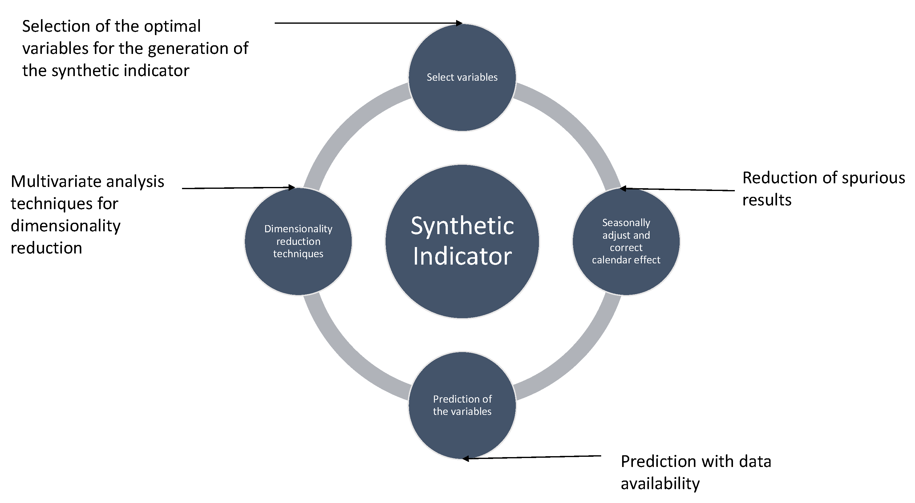
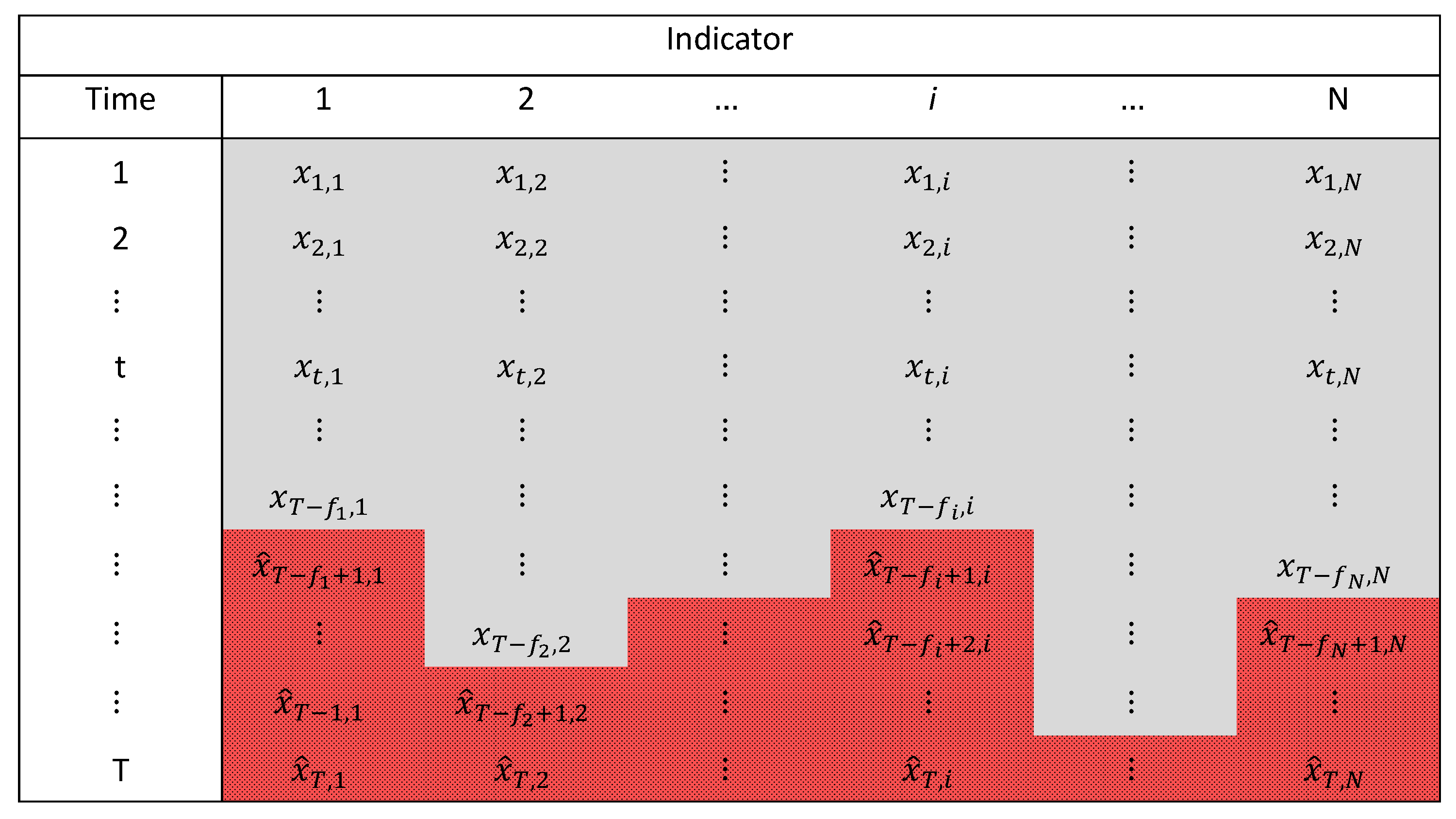
3.1. Synthetic Index

The construction of a synthetic index is dependent on its purpose for being built, and on the simple indicators that it is composed of and how these combine; all these ingredients interact dynamically to produce a solution (see Figure 1).

In our case, the objective is to build a high-frequency (monthly) synthetic index capable of capturing the aggregate economic evolution of the Comunitat Valenciana. The purpose is to increase—without delay and synthetically—our knowledge of the current experience of the regional economy (nowcasting) and predict its immediate future behaviour (short-term forecasting). Our reference index (that is, its components) should therefore be related to the gross domestic product (GDP) of the Comunitat Valenciana. Unfortunately, as mentioned in the previous section, regional GDP series are only available annually and, as is usually the case in many countries [9], with a significant time delay. Therefore, bearing in mind our objective of developing a monthly index, the first issue to be addressed is how to compare/relate the potential elementary indicators to the reference series. Of the two available solutions—either temporally aggregating the monthly series and studying the annual frequency relationships or disaggregating the annual series and studying the monthly frequency relationships— we opted for the second solution. The possibilities for analysis are richer and the sample sizes greater. Specifically, we use the temporary disaggregation methodology of the high frequency of Dagum and Cholette [31], which monthly interpolate the annual series subject to the annual aggregation constraint.

The new monthly GDP series is used in the empirical part of this study to quantify/objectify the criteria of representativeness and significance in the selection of simple indicators. This is less restrictive than it might seem at first glance. From a methodological perspective, it does not presuppose anything about which initial indicators should be considered or how the selected indicators should be combined. From a procedural perspective, the app presented in this study can be used by any researcher/analyst to build their own synthetic index, using their own indicators chosen according to their own criteria. Furthermore, from a substantive perspective, simple indicators are not chosen to replicate/predict the artificial series of GDP which was built, but rather because they provide relevant information about the overall economic evolution. The introduction of the indicators in the elaborated synthetic index is sufficiently flexible to allow the high-frequency movements of the simple indicators to report on the changes that are occurring in the economic future. The monthly GDP series which was built does not contain this information.

Together with the criterion of representativeness and high significance, in our empirical application, the initial selection of indicators reflects, from a previous selection based on expert knowledge, the criteria of availability, frequency and delay. The indicators must be available with little delay, the cost of obtaining them must be low and their frequency of update must be high—preferably monthly.

Once an initial set of indicators is chosen, this can be refined using variable selection methods, two of which are the “subset selection” methods (forward and backward included) and regularisation methods [32,33,34]. The subset selection methods are based on the identification of the subset variables that together best predict/explain the response variable, or at least the identification of a good subset. The regularisation methods Ridge, Lasso or Elastic Net select the features indirectly, adjusting a model with all the predictors which incorporates a penalty that punishes the coefficients (approaching them to zero) associated with the variables that provide little predictive capacity. In our empirical application, we use a complete subset selection method.

Once the final set of simple indicators is selected, the construction phase of the synthetic index begins. There are multiple methods of aggregating indicators [35], from the simplest based on a fixed weighting structure, exogenously determined or according to some univariate criteria, to more complex methods based on the main component techniques and factor analysis. Many of these methods, however, face the problem of asynchrony presented by economic series in terms of their cyclical information. Not all series can be considered synchronous with the economic cycle; we find leading, lagging and coincident series. The series, therefore, need to be dated and delayed/advanced in order to be synchronised [36]. Some of the studies that address this problem, within the framework of building synthetic indexes, are those of Mondéjar-Jiménez and Vargas-Vargas [37], Domínguez Serrano et al. [38] and Cuevas and Quilis [39]. All of these propose indicator aggregation techniques through main components and factor analysis, offering a literature review of the existing aggregation methods. See also Doz and Fuleky [40].

One way to ignore the problem of date (temporal synchronisation) is to use dynamic factor analysis methods. Dynamic factorial analysis techniques incorporate the dynamics of the series in their search for the set of the time signals common to all series. Specifically, our application takes the research by Cuevas et al. [36] as a reference and uses the dynamic factor analysis to reduce the dimensionality of the problem and discover a single latent factor (the first dynamic factor) that represents the original variables with the least loss of information. The complete process is shown in Figure 1, which includes the phase of treatment and univariate prediction of the series, addressed below. The implemented model allows new observations of simple indicators to be incorporated according to the availability of the data.

Following the procedure described in Figure 1, for the calculation of the synthetic indicator, given an initial set of time series, a set of N time series is selected using the subset selection method. These series are all completed up to the same moment in time using univariate prediction methods. They are previously corrected of calendar effects and seasonally adjusted. Various previous analyses (not presented in this paper) reveal that the univariate prediction of the elementary indicators offers better results and flexibility than the predictive extension of the dynamic factor itself, whether it is performed exogenously (prediction after univariate modelling), or endogenously, during the process of its calculation through dynamic factor analysis.

In our research, the treatment and correction of seasonal, outlier and calendar effects of simple indicators is carried out using the methodology described in JDemetra+ [41]. Specifically, as a complement to the synthetic indicator app, there is an alternative app that allows each series to be processed using the TRAMO-SEATS [42] or X-13ARIMA-SEATS [43] methodology, based on an identification (defined by the user or automatic) of the autoregressive integrated moving average (ARIMA) model of the series to be treated. An advantage of this alternative app, other than the simplicity of its use, is that, in addition to the usual calendar correction components (moveable Easter effect, weekly cycle or leap year), it allows the incorporation of other components built from the festive and commercial calendar of the Comunitat Valenciana [44]. Like the main app (for the construction of the synthetic indicator), this app https://apps.uv.es/app_extraccion_componentes/ (accessed on 17 April 2023) may also be of interest to other analysts.

It is common for elementary indicators to not all be available at a certain time point and, furthermore, prior to the current time (nowcasting) and certainly prior to the time up at which we want to make a prediction (short-term forecasting). For this reason, imposing a restriction regarding the maximum number of months that each series can be predicted (which we set at a maximum of 12 months with respect to the most delayed series), each series is predicted until all of them are located at the same time instant (see Figure 2).

Figure 2 schematically shows the observed and predicted data structure for each series; where $x_{t,i}$ represents the observed value of the i-th indicator during instant t and ${\widehat{x}}_{T-f_i+k,i}$ represents the prediction associated with the i-th indicator corresponding to the instant $T-f_i+k$ (with, $f_i\ge k$), with T denoting the total number of periods (the time horizon), N denoting the number of elemental indicators and $f_i$(≤12) denoting the number of unobserved periods (months) (to be predicted) until the i-th series is completed at instant T.

In our application, each series/indicator is completed/predicted using automatically identified univariate ARIMA models. The model identification (and prediction) process is performed using the Box–Jenkins methodology (see, e.g., [45]). The greatest advantage provided by this type of model, compared to other more sophisticated ones, usually resides in its ability to generate optimal predictions for the immediate future [46]. Of course, the analyst can choose to use an alternative forecasting procedure working with already complete/predicted series before the construction of the synthetic index.

Once a complete/completed data matrix is available, such as the one shown in Figure 2, the synthetic index ($IS$) is estimated using dynamic factorial analysis, as in Cuevas et al. [36], after applying a series of transformations to the series to eliminate their scale differences and ensure that they are stationary with an approximate normal distribution. Specifically, the app performs in each indicator series: (i) a logarithmic transformation to ensure the normality and symmetry of the data; (ii) a differentiation to eliminate the trend components of the series; and (iii) a standardisation of the variables to homogenise their scales and variances.

Dynamic factor analysis allows each series to be expressed as a linear function of a set $r<<N$ of common factors, which captures the patterns of co-movements shared by all series, and some idiosyncratic effects specific to each series. In our approximation, $r=1$.

Mathematically, the relationships can be expressed for $t=1,\dots ,T$ through Equations (1) and (2).

$${\mathit{x}}_{\mathit{t}}=\mathit{\lambda }\left(\mathit{L}\right){\mathit{f}}_{\mathit{t}}+{\mathit{\epsilon }}_{\mathit{t}}$$

(1)

$$f_t=\mathrm{\Psi }\left(L\right)f_{t-1}+{\eta }_t$$

(2)

where ${\mathit{x}}_{\mathit{t}}$ and ${\mathit{\epsilon }}_{\mathit{t}}$ are vectors of dimension $N\times 1$ (N being the number of indicators and ${\mathit{\epsilon }}_{\mathit{t}}$ being the vector of specific or idiosyncratic components of the indicators at time t), $f_t$ is the r-dimensional factorial vector which captures the values of the factor at the instant t, ${\eta }_t$ a random r-dimensional white noise vector and $\lambda \left(L\right)$ and $\mathrm{\Psi }\left(L\right)$ are matrix delay polynomials of dimensions $N\times r$ and $r\times r$, respectively, where L is the lag operator.

On the one hand, the i-th delay polynomial ${\lambda }_i\left(L\right)$, that is, the i-th row of $\lambda \left(L\right)$, denotes the loading of the factor for the i-th series and ${\lambda }_i\left(L\right)$ $f_t$ denotes the common component of the i-th series. The loadings polynomic ${\lambda }_i\left(L\right)$ measures the sensitivity of the growth signal of the i-th indicator for changes in the factor. On the other hand, the polynomial lag matrix $\mathrm{\Psi }\left(L\right)$ captures the dynamic structure of common factors.

The above system is estimated under the classical assumptions of stationarity for Equations (1) and (2), assuming that the idiosyncratic components are uncorrelated with all factors at all lags, that is, $E\left[{\epsilon }_{t,i}{\eta }_{t-k,j}^{\prime }\right]=0\forall i,j,k$. Once the system has been estimated, the dynamic factorial model provides us with the communality corresponding to the first factor; from which we derive the synthetic index in base one by means of Equation (3), where $I{S}_1=1$

$$I{S}_{t+1}=I{S}_t(1+f_t)$$

(3)

3.2. Uncertainty Measurement

The second of our objectives is to generate the precision measures of the synthetic index to measure its uncertainty. From a classical frequentist perspective, the uncertainty of a statistic is measured by accounting for the uncertainty associated with the sample used for its construction. On many occasions, however, as in macroeconomics, it is not possible to have different samples of the same variable or to repeat a study a great number of times. In these circumstances, uncertainty is measured based on the assumptions of the model that is used to solve the problem or after assuming a certain generating structure for the data, as occurs in the context of ARIMA time series modelling.

The construction of a synthetic index using dynamic factor analysis, however, entails very complex mathematical operations that are difficult to trace, which prevent the error structures from being analytically transferred through the system. In these contexts, as well as in general, it is possible to use simulation techniques to solve the problem: resampling techniques from which we can obtain the estimates of standard errors, confidence intervals or resolve hypothesis tests. In this research, we use the bootstrap methodology (see, e.g., [47]).

According to Efron and Tibshirani [29], the relationship between the original sample and the bootstrap is explained by the connection between two worlds, the real world and the bootstrap world. In the real world, the joint multivariate probability distribution, F, of the phenomenon under study, is unknown, and a random sample is available, $\mathit{x}=\left(x_1,\dots ,x_n\right)$, which is used to estimate a statistic of interest $\widehat{\theta }=s\left(\mathit{x}\right)$. In the bootstrap world, the empirical distribution $\widehat{F}$ of the data is obtained by resampling with replacement the observed sample (or the estimated errors) of the real world, ${\mathit{x}}^{*}=(x_1^{*},\dots ,x_n^{*})$, using this estimate of the empirical distribution to obtain parameters of interest that would be impossible to obtain in the real world.

In our case, dynamic factor analysis is a deterministic process: given the same inputs, the same output is always obtained. In other words, contingent upon the observed values of the elementary indicators, the synthetic index is invariant: it is not subject to any uncertainty. There are, however, two sources of uncertainty that could be introduced into the process. On the one hand, the elementary indicators are approximations to reality and are subject to measurement errors. On the other hand, as previously stated, the nowcasting and forecasting objectives impel the use of univariate predictions to complete the series of indicators (see Figure 2). This is a process subject to uncertainty which also grows as the prediction time horizon increases.

Although we do not include the uncertainty associated with the first source in this research because the observed values are considered fixed according to a model-based approach [48], we can suggest at least two strategies for those researchers that are interested in incorporating it. On the one hand, the observed series could be locally perturbed, retaining the dependency structure of the data, using the (linked) blockwise bootstrap (see, e.g., [49]). On the other hand, the errors associated with the ARIMA modelling of the indicators could be used to generate new series as a composition of observed values and resampled errors.

The second source of uncertainty (the one associated with the univariate prediction of each base indicator) is incorporated into the process and, given the dynamic structure of the built factor, it ends up having an impact on all the time instants of the index, not only on the instants in which a prediction has been made. The uncertainty associated with the specific predictions of each indicator series is incorporated by building new series as a concatenation of the observed values of the series and replicas of the predictions obtained by sampling in their associated prediction intervals.

Mathematically, continuing with the notation introduced in the previous subsection, the process starts from the observed values $(x_{1,i},x_{2,i},\dots ,x_{t,i},\dots ,x_{T-f_i,i})$ and varies the predictions ${\widehat{x}}_{T-f_i+k,i},k=1\dots f_i$ of each series in each resample. To do this, denoting by ${\widehat{x}}_{T-f_i+k,i}^{-}$ and ${\widehat{x}}_{T-f_i+k,i}^{+}$, the minimum and maximum values (obtained, for example, from a prediction interval with a given confidence) among which the prediction for the instant $T-f_i+k$ of the i-th series would reasonably be found, we randomly extract a value $x_{T-f_i+k,i}^{*}$ from the interval $[{\widehat{x}}_{T-f_i+k,i}^{-},{\widehat{x}}_{T-f_i+k,i}^{+}]$, for $k=1,\dots ,f_i$, and construct a new series such as: $x_{1,i},x_{2,i},\dots ,x_{t,i},\dots ,x_{T-f_i,i},\dots ,x_{T-f_i+k,i}^{*},\dots x_{T,i}^{*}$. This process is repeated B times for each of the N series. Specifically, for $b=1,\dots ,B$ and $i=1,\dots ,N,{\mathit{x}}_i^{\left(b\right)}=(x_{1,i},x_{2,i},\dots ,x_{t,i},\dots ,x_{T-f_i,i},\dots ,x_{T-f_i+1,i}^{*\left(b\right)},\dots ,x_{T,i}^{*\left(b\right)})$ denotes the b-th resample of the i-th indicator series and ${\mathit{X}}^{\left(\mathit{b}\right)}=\left[{\mathit{x}}_{\mathbf{1}}^{\left(\mathit{b}\right)},{\mathit{x}}_{\mathbf{2}}^{\left(\mathit{b}\right)},\dots ,{\mathit{x}}_{\mathit{i}}^{\left(\mathit{b}\right)},\dots ,{\mathit{x}}_{\mathit{N}}^{\left(\mathit{b}\right)}\right]$ denotes the indicator matrix of order $T\times N$ corresponding to the b-th resample.

At this point, we have B matrices, ${\mathit{X}}^{\left(\mathit{b}\right)}$ $b=1,\dots ,B$, of simple indicators. The synthetic index construction procedure described in the previous subsection is applied to each of these, obtaining B series of synthetic indicators: $I{S}^{\left(1\right)},I{S}^{\left(2\right)},\dots ,I{S}^{\left(b\right)},\dots ,I{S}^{\left(B\right)}$. All of these share the same probability distribution, so that they can be considered as a simple random sample, ${\mathit{IS}}^{*}=(I{S}^{\left(1\right)},\dots ,I{S}^{\left(b\right)},\dots ,I{S}^{\left(B\right)})\stackrel{\mathrm{iid}}{\sim }{\widehat{F}}_{IS}$, from which we can extract the estimates of the mean synthetic index, the standard error associated with each time instant, or construct confidence intervals for the value of the synthetic index, $t=1,\dots ,T$.

In particular, denoting by $I{S}_t^{\left(b\right)}$ the value of the synthetic index obtained for instant t with the b-th resample, the estimator of the average synthetic index—whose expected value will coincide with the IS index obtained in the previous section—and its associated standard deviations at each instant are obtained, following [29], using Equations (4)–(6):

$$\overline{IS}=\left({\overline{IS}}_1,{\overline{IS}}_2,\dots ,{\overline{IS}}_t,\dots ,{\overline{IS}}_T\right)$$

(4)

where

$${\overline{IS}}_t=\sum _{b=1}^B\frac{I{S}_t^{\left(b\right)}}{B}$$

(5)

and

$${\widehat{\sigma }}_{{\overline{IS}}_t}=+\sqrt{\frac{{\sum }_{b=1}^B{\left(I{S}_t^{\left(b\right)}-{\overline{IS}}_t\right)}^2}{B-1}}$$

(6)

There are two possibilities for building confidence intervals. One is to assume a normal distribution for the values of the synthetic index at each instant, and the other is to directly use the bootstrap confidence intervals. The first approximation involves calculating the intervals by $[{\overline{IS}}_t\pm z_{\frac{\alpha }{2}}{\widehat{\sigma }}_{{\overline{IS}}_t}]$, where $z_{\frac{\alpha }{2}}$ is the percentile $1-\alpha /2$ of a standard normal distribution. The second strategy estimates the confidence interval, with $1-\alpha$ confidence, for the value of the index at instant t from the bootstrap percentiles, Equation (7).

$$\left[I{S}_t^{\alpha /2},I{S}_t^{1-\alpha /2}\right]$$

(7)

where $I{S}_t^{1-\alpha /2}$ denotes the $1-\frac{\alpha }{2}$ percentile of the bootstrapped synthetic index during period t. These percentiles are obtained as the values of the set $\{I{S}_t^{\left(1\right)},I{S}_t^{\left(2\right)},\dots ,I{S}_t^{\left(b\right)},\dots ,I{S}_t^{\left(B\right)}\}$ below which $\left(\alpha /2\right)\%$ and $\left(1-\alpha /2\right)\%$ of the values are found, respectively.

4. Synthetic Index: Web Application

The synthetic index construction methodology is complex and involves a series of laborious operations that, fortunately, can be automated. The automation of these processes facilitates economic decision making, particularly for regional public agents whose statistical and computational skills are often limited. Hence, in accordance with one of the objectives of this research, we develop an easy-to-use interactive application to build a synthetic index, given a set of indicators, using the dynamic factor analysis methodology described in the previous section. The application was developed using the R programming language [50], common in research areas for statistical analysis, employing the Shiny package [51], which simplifies the building of interactive applications.

The “Synthetic Indicator” application developed with Shiny (see Figure 3) is composed of two functional components: a user interface (UI) function and a server function (SERVER). The UI function is responsible for generating the visible part of the interactive web and is the one that contains the visual structure. The SERVER function is in charge of the mechanical and internal execution of the interactive web and contains the instructions for the application.

The application has three tabs. The first one, called “Introduction”, briefly explains the objective of the application and its main results. The second tab is the generator of the synthetic indicator of economic growth. In this second tab, the interactive web asks the user for various inputs, such as the date (month and year) up to which they want the synthetic indicator to reach, as well as one (or two) Microsoft Excel file(s) with the monthly and/or quarterly indicators that the user wants to combine to build the synthetic indicator. The first column of these files contains the dates in YYYYMMM format (for example, 2022M12) for monthly series and in YYYYTQ format (for example, 2023T2) for quarterly series. The data, with a name heading for each series, are located in the columns that follow. Since the indicator is built on a monthly basis, the quarterly series (if introduced) are interpolated on a monthly basis using [31]. Finally, the app asks the user to decide which option to use to combine the indicators in terms of start date: “default-observed series” or backcasting. The backcasting option performs a backward point estimate of all the economic indicators until completing them up to the date of the indicator for which the oldest date is available. The default option starts all the series, taking as the start date the oldest date for which there are known observations for all the series.

Once the user enters these inputs, the application shows the values of the generated synthetic indicator as output and displays a graphical representation of it on the screen. The user can download the data in a file in .xlsx format.

The application https://apps.uv.es/app_indicador_sintetico/ (accessed on 17 April 2023) also has a third tab that contains the user manual, providing a step-by-step explanation in Spanish of how to create a synthetic indicator of regional economic growth.

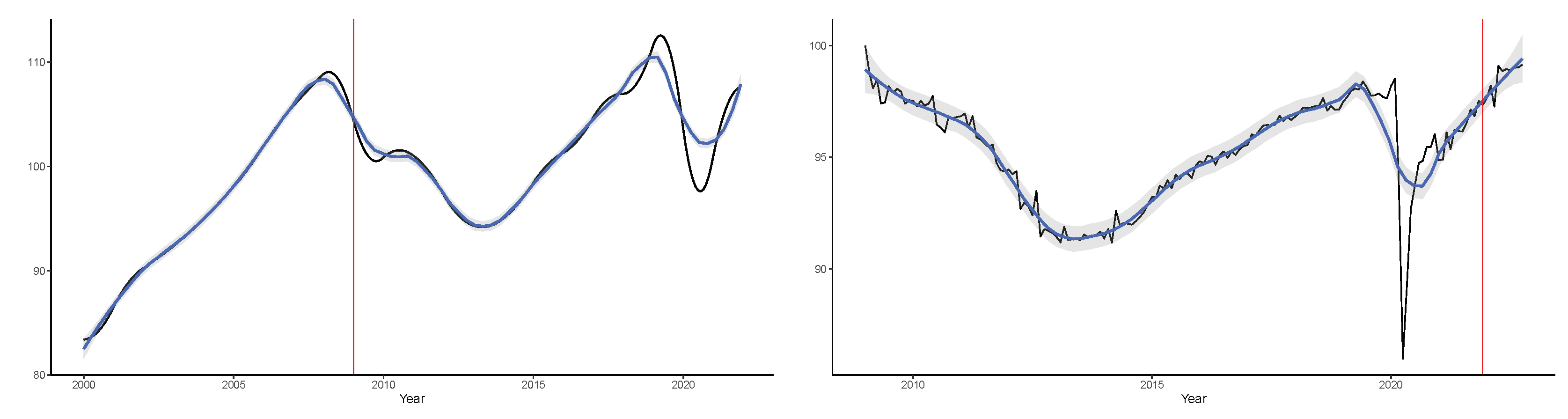
5. Empirical Application

The use of simple economic indicators to monitor economic cycles is very useful for measuring the effectiveness of the public policies that are being implemented [9,35]. Each indicator gives information about the past and the situation of the phenomenon it captures, projecting its evolution into the present and future. However, the information provided by the indicators is partial and sometimes contradictory. Different indicators may be found at different times in the cycle (for example, the unemployment rate tends to improve some time after an improvement in the cycle has occurred, while an increase in the demand for business financing usually brings forward an improvement in the cycle). Alternatively, the underlying phenomena that the indicators measure may present different evolutions. To overcome this limitation, we must resort to aggregation methods that allow us to measure the unobservable latent variables of the set of indicators.

With the objective of building an indicator highly correlated with the GDP of the Comunitat Valenciana and paying particular attention to criteria such as the availability of the variable and its high statistical significance, in this research, we initially selected 14 indicators to build the synthetic index, as detailed in

Table 1. Simple indicators initially considered to build the synthetic index.

Code	Description
AFSST	Total affiliated to the social security system
AFSSC	Total affiliated to the social security system in the construction sector
CPPT	Consumption of petroleum products
CVV	Property sales
EXPORT	Exports
GTOTUR	Tourist spending
IASS	Service sector activity indicator
ICMG	Retail turnover index
IMPORT	Imports
IPI	Industrial production index
MATTUR	Vehicle registrations
MATVC	Heavy-duty vehicle registrations
PHT	Total overnight stays in hotel establishments
VET	Total approvals of building certificates

. The official source producing all the indicators is the Spanish Statistical Office (INE).

Although the 14 individual indicators could be combined into a single synthetic index, based on the principle of parsimony and our objective of representativeness of the index in terms of GDP, as indicated in the methodology section, we make a prior selection of indicators using “subset selection”. Using the AIC criterion, we identify the subset of indicators that together provide a lower AIC in relation to GDP. The main advantage of performing a preselection lies in the reduction in the complexity and computational costs. Prior to applying the “subset selection” method, the annual series of GDP is transformed into a monthly one by applying [31] and the monthly series of elementary indicators are standardised to avoid scale effects.

In this specific case, since we have 14 independent variables/predictors, $2^{14}-1=\mathrm{16,383}$ different models are fitted, after considering all possible combinations with at least one predictor. An extract with a statistical summary with three of the fitted models is presented in

Table 2. Statistical summary of an extract of models in the subset selection.

Model	N	Predictors	${\mathit{R}}^2$	Adj. ${\mathit{R}}^2$	AIC
9908	8	AFSST GTOTUR IASS ICMG	0.94	0.94	15.31
		IMPORT MATTUR MATVC PHT
⋯	⋯	⋯	⋯	⋯	⋯
16,383	14	AFSST AFSSC CPPT CVV EXPORT	0.94	0.94	23.12
		EXPORT GTOTUR IASS ICMG IMPORT
		IPI MATTUR MATVC PHT VET
⋯	⋯	⋯	⋯	⋯	⋯
14	1	CPPT	0.13	0.12	361.72
⋯	⋯	⋯	⋯	⋯	⋯

. The last column of Table 2 shows the values for the coefficient $AIC=2k-2ln(\widehat{L})$ obtained for each model, where k is the number of estimated parameters (as an indicator of complexity) of the model and $\widehat{L}$ is the maximised value of the likelihood function for the model. According to the criterion of the lowest AIC, the selected model would be the one labelled with the number 9908 which contains eight indicators. As can be seen, most of the selected indicators are indicators of demand and of the services sector.

As shown in Table 2, in terms of fit, there are no major differences between the most parsimonious model selected and the most complex model built by linearly combining the 14 indicators. This is due to the prior selection of the initial indicators, for which expert knowledge was used. Indeed, the results of this application can be considered robust since almost the same synthetic index is obtained if the 14 initial selected indicators had been employed.

The result of calculating the synthetic index using the app option “observed data” with the eight indicators selected in model 9908 is shown in the left panel of Figure 4 during the period January 2009–October 2022. As an element of comparison, in the right panel of Figure 4, the monthly GDP series of the Comunitat Valenciana, available until 2021, is graphically represented. In both panels, a smooth LOESS curve is included to make it easier to observe their underlying evolutions. Likewise, vertical red lines are used in both panels to indicate the periods during which the other series is (not) available.

As can be seen by comparing both panels of Figure 4, during the intersection period (when both series are available), the movements of both curves are quite similar—an indicator of the usefulness of the synthetic index, for which we have nowcast and forecast estimates. In both curves, the economic consequences of the lockdown implemented to mitigate the COVID-19 pandemic are evident. Remarkably, the huge drop in economic activity caused by the lockdown is more evident in the synthetic index than in the monthly GDP series. On the one hand, there was a statistical smoothing effect caused by the monthly disaggregation method and, on the other hand, the significant financial aid that accompanied the lockdown made it possible to maintain a significant degree of consumption despite the reduction in activity.

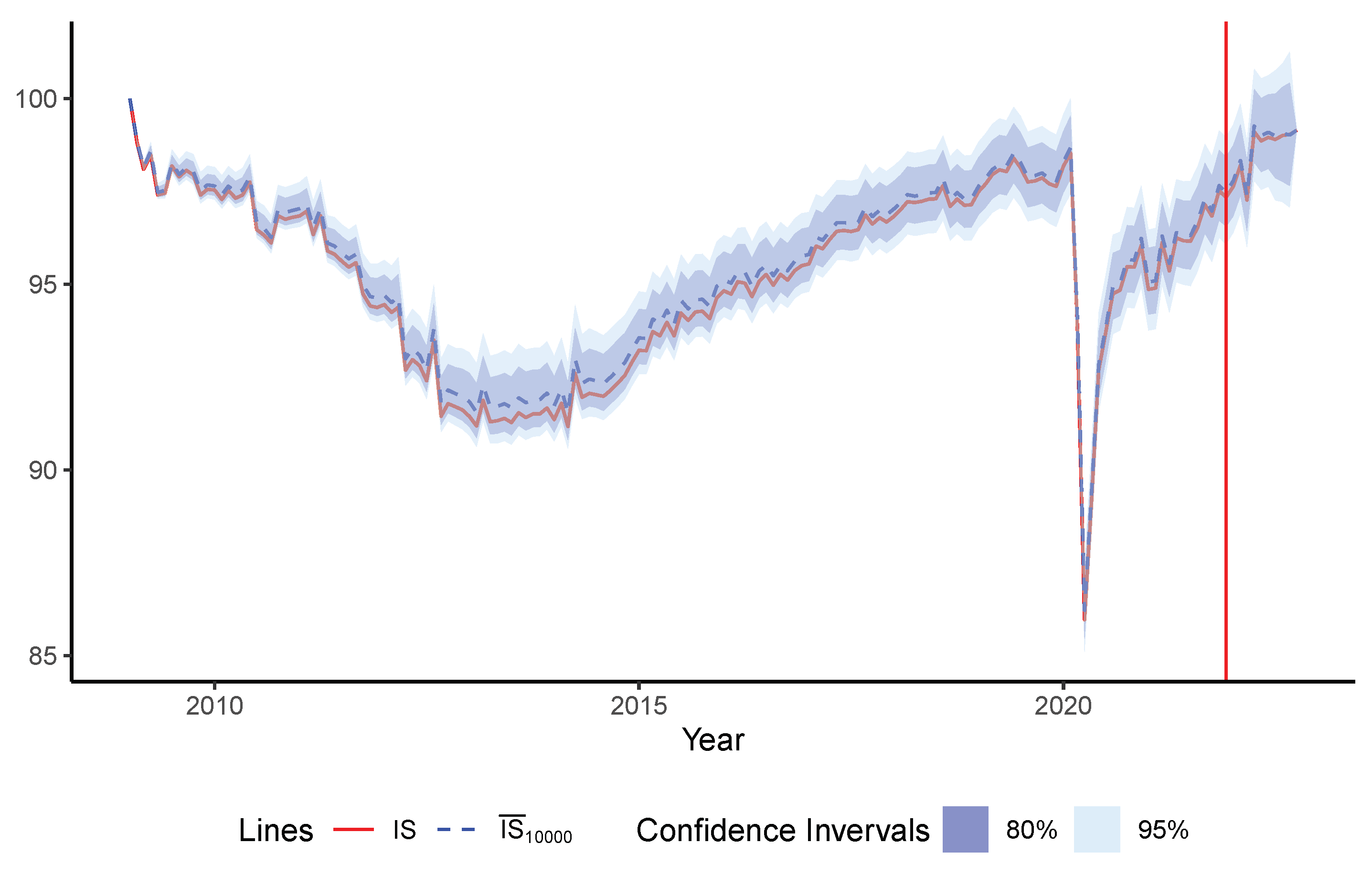
6. Measuring the Uncertainty

A prediction or estimate is not complete without a measurement of its prediction/estimate error, that is, the level of uncertainty associated with it. The calculation of uncertainty is not always straightforward, as is the case with the construction of our synthetic index that employs dynamic factor analysis. Fortunately, as discussed in the methodology section, simulation techniques can (almost) always be used to generate estimates of uncertainty. In this section, we show (as can be seen in Figure 5) the results of measuring the uncertainty associated with the construction of the synthetic index using the procedure described in Section 3.2 for $B=\mathrm{10,000}$.

Figure 5 graphically shows the synthetic index together with the estimation of its bootstrap confidence intervals at 80% and 95% confidence. Several facts stand out when analysing this figure. First, the uncertainty bands are not homogeneous during the entire period. During the initial years and at the time of the pandemic lockdown, the levels of uncertainty are lower. The highest levels of uncertainty are observed during the prediction/extrapolation period. Second, the bootstrap intervals are not symmetric with respect to the base index, $IS$, nor with respect to the mean index, $\overline{IS}$, with the intervals being significantly more asymmetric with respect to the former. In general, the interval range towards the upper end is greater than it is towards the lower end. Third, as a rule, the index series $IS$ and $\overline{IS}$ nearly coincide, drawing very similar paths. In summary, the bootstrap methodology is revealed to be adequate to approximate uncertainty in the estimation of the synthetic index of activity and economic forecast of the Comunitat Valenciana.

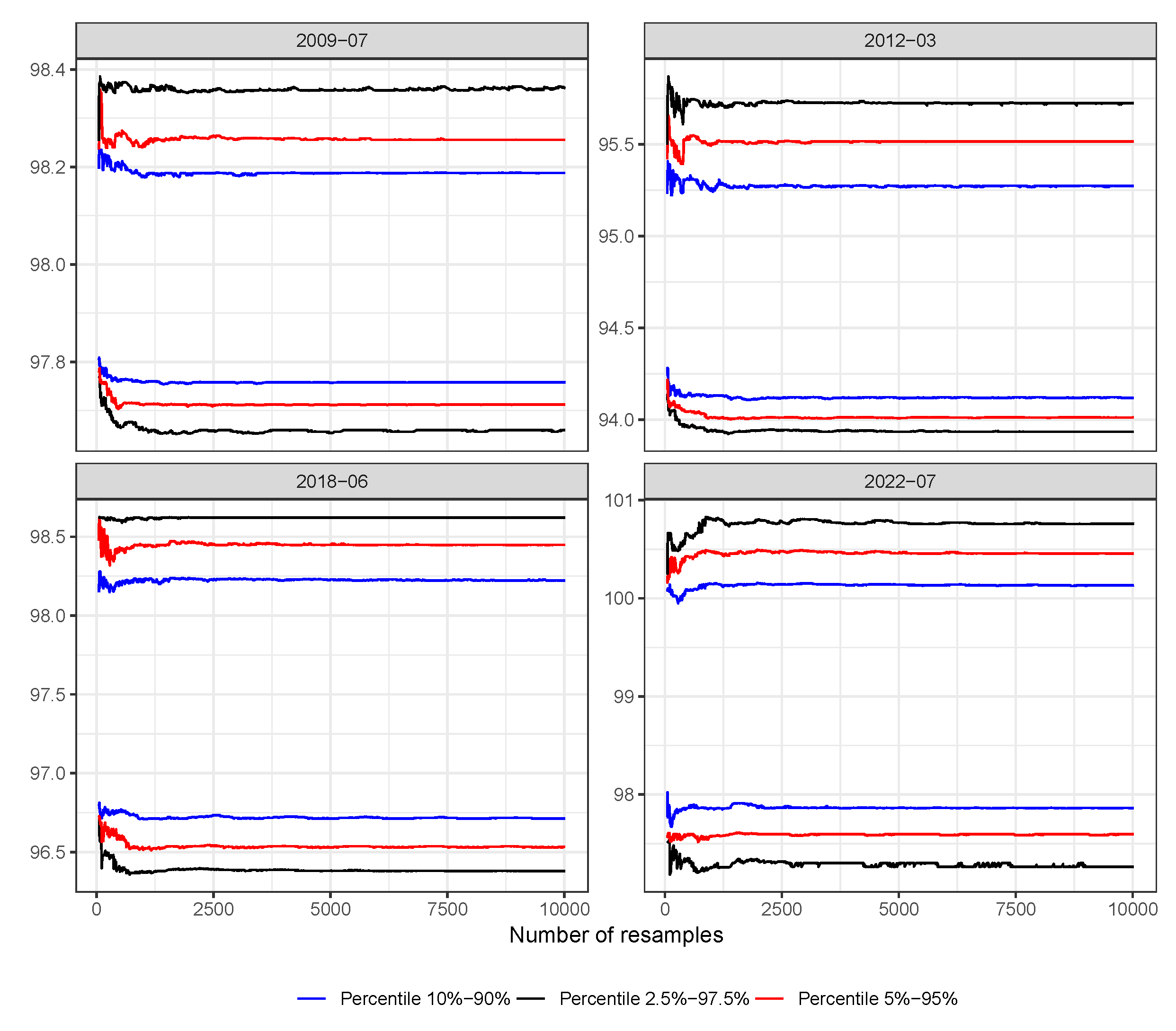
7. How Many Resamples? An Analysis of Sensitivity

The previous section concludes that the bootstrap simulation is a good alternative for measuring uncertainty when we combine different economic series through dynamic factor analysis. In the previous application, however, we used 10,000 simulations, which incurred a high computational cost (high processing times and cycles), even when using parallel processing systems that reduce computing times. The natural question that arises is whether it is necessary to perform so many simulations. In other words, what would be the minimum number of resamples necessary to guarantee the convergence of the confidence intervals?

Knowing the minimum number of simulated scenarios necessary to achieve stability in the estimate of the standard errors and confidence intervals is relevant because, on the one hand, this would allow us to be sure of the estimates obtained and, on the other hand, it would avoid wasting resources by incurring an excessive computational cost with unnecessary calculations. Providing an answer to this question is the second of the contributions of this paper.

In the literature, however, there is no consensus regarding what should be the minimum number of resamples to achieve stability in the estimates. Efron and Tibshirani [29] affirm that with a relatively low number, such as 50 or even 25 resamples, we could achieve stability in the estimation of the standard error, although the number of resamples necessary to estimate the confidence intervals would be somewhat higher. Other authors such as Wilcox [52] recommends using a minimum of 599 simulations as a general rule, while Davidson and MacKinnon [53] defended that the optimal minimum number for B must be reasonably large. In practice, Davidson and MacKinnon [53] stated that using 399 simulations would be sufficient, although they recommend using a larger number if we wish to increase the power and precision in estimating the estimation error and confidence intervals with $1-\alpha =0.95$.

Other authors are more conservative. Hesterberg [30] considers that 1000 resamples are necessary to achieve stability in the error estimate and recommends the use of 10,000 resamples when the objective is to estimate confidence intervals with sufficient coverage. Finally, Chernick [54] states that there is no fixed number of resamples that guarantees reaching average convergence.

In order to answer the questions raised in the context of this research, we simulated $B=\mathrm{10,000}$ resamples—a number above that recommended by [52,53] and equal to that recommended by [30]—and (i) studied, as a function of the number of resamples b, when stability is reached; and (ii) compared the differences observed between the limits of the intervals obtained for different numbers of resamples, $b=\left\{25,50,399,599,1000,\mathrm{10,000}\right\}$. The analyses were also carried out considering the possible impact of the coverage $(1-\alpha )$ of the interval used in the results. Indeed, as shown in Figure 6, where the limits of the confidence intervals obtained for the synthetic index at four different time points are shown as a function of the number of resamples b, not all the interval limits tend to stabilise in the same number of resamples.

To study when stability is reached at the limits of the confidence intervals, we use linear regressions with the independent variable being the number of resamples and the dependent variables being the limits of the intervals: ${\ell }_t^{\left(b\right)}=\alpha +\beta b$ for $b\ge b_0$, where ${\ell }_t^{\left(b\right)}$ represents, for instant t, any one of the limits of the confidence interval of the index obtained using the first b resamples.

Given that, logically, the bootstrap percentiles tend to stabilise as the number of resamples increases, the calculation of the p-values associated with the coefficients $\beta$ for $b\ge b_0$ indicates from which resample number $b_0$ the coefficient $\beta$ is no longer statistically significant. From this number, we can say that the corresponding set of limits has stabilised since the regression line is well fitted by way of a constant.

Adopting a conservative criterion, according to which we need at least as many resamples as the maximum number of resamples required to reach stability at all time points, it follows that, for the usual confidence levels $\left(1-\alpha =0.80,0.90,0.95\right)$, we would need to simulate almost 10,000 resamples. This statistical result is not very useful from a practical point of view because, as shown in Figure 6, practical stability is generally reached much earlier.

In order to answer the question from a practical perspective, we compare the limits obtained for the different pairs of resampling number combinations and analysing the errors and standard deviations associated with their differences. For each possible combination of the set $\mathrm{\Omega }=\{25,50,399,599,1000,10000\}$, we calculate across periods the statistics $s{d}_t\left({\ell }_t^{\left(b_1\right)}-{\ell }_t^{\left(b_2\right)}\right)$ and $s{d}_t\left({\ell }_t^{\left(b_1\right)}-{\ell }_t^{\left(b_2\right)}\right)/mea{n}_t\left({\ell }_t^{\left(b_2\right)}\right)$, where $b_1,b_2\in \mathrm{\Omega }$ and $b_1<b_2$.

Table 3. Standard deviations (left panel) and relative errors in percentages (right panel) across time between confidence interval limits at 90% (upper triangles) and 10% (lower triangles) for a selected number of resamples.

	25	50	399	599	1000	10,000		25	50	399	599	1000	10,000
25		0.1018	0.0991	0.1001	0.1034	0.0985			0.1058	0.1029	0.1040	0.1074	0.1023
50	0.1171		0.0352	0.0439	0.0629	0.0590		0.1232		0.0365	0.0456	0.0653	0.0612
399	0.0969	0.0688		0.0195	0.0460	0.0405		0.1020	0.0724		0.0203	0.0477	0.0420
599	0.0954	0.0683	0.0098		0.0312	0.0260		0.1005	0.0719	0.0103		0.0324	0.0270
1000	0.1124	0.0682	0.0254	0.0247		0.0114		0.1183	0.0718	0.0267	0.0260		0.0118
10,000	0.1079	0.0704	0.0181	0.0177	0.0106			0.1136	0.0742	0.0191	0.0186	0.0112

,

Table 4. Standard deviations (left panel) and relative errors in percentages (right panel) across time between confidence interval limits at 95% (upper triangles) and 5% (lower triangles) for a selected number of resamples.

	25	50	399	599	1000	10,000		25	50	399	599	1000	10,000
25		0.0858	0.1149	0.1373	0.1270	0.1260			0.0890	0.1190	0.1422	0.1315	0.1305
50	0.0623		0.0701	0.0904	0.0951	0.0963		0.0656		0.0726	0.0936	0.0985	0.0997
399	0.0855	0.0868		0.0396	0.0518	0.0508		0.0901	0.0915		0.0410	0.0537	0.0526
599	0.0892	0.0837	0.0205		0.0595	0.0578		0.0940	0.0883	0.0217		0.0616	0.0598
1000	0.1006	0.0861	0.0438	0.0305		0.0119		0.1061	0.0908	0.0463	0.0322		0.0123
10000	0.0999	0.0887	0.0345	0.0232	0.0140			0.1053	0.0936	0.0364	0.0245	0.0148

and

Table 5. Standard deviations (left panel) and relative errors in percentages (right panel) across time between confidence interval limits at 97.5% (upper triangles) and 2.5% (lower triangles) for a selected number of resamples.

	25	50	399	599	1000	10,000		25	50	399	599	1000	10,000
25		0.1178	0.1112	0.1160	0.1437	0.1483			0.1219	0.1150	0.1199	0.1485	0.1532
50	0.1031		0.1263	0.1241	0.1280	0.1310		0.1085		0.1305	0.1282	0.1323	0.1354
399	0.0911	0.0859		0.0238	0.0558	0.0618		0.0961	0.0906		0.0246	0.0577	0.0638
599	0.0970	0.0874	0.0191		0.0970	0.0874		0.1024	0.0922	0.0202		0.0487	0.0531
1000	0.1029	0.0926	0.0245	0.0181		0.0142		0.1087	0.0978	0.0258	0.0191		0.0147
10,000	0.1059	0.0913	0.0286	0.0212	0.0126			0.1119	0.0964	0.0302	0.0224	0.0133

show the values obtained for such statistics associated with the confidence intervals at 80, 90 and 95 %, respectively.

The analysis of the values of the tables shows that the lower limits of the intervals presented greater stability than the upper limits and that, in addition, their relative error reaches a value close to 1% relatively quickly. The mean distances across periods between the lower limits are practically equivalent for 399 resamples. For the upper limits, however, we need approximately 1000 resamples to achieve limits similar to those obtained with 10,000 resamples. In light of these results, we consider that, in this context, it is more than enough to take 1000 resamples to calculate the confidence intervals for the synthetic index at the different time points.

8. Summary and Final Remarks

Economic agents, both public and private, have the responsibility to make decisions on a daily basis that can have important social and financial consequences. These decisions are made based on current and future conditions. Therefore, having adequate tools for conjunctural analysis, economic forecasting and measuring uncertainty constitutes a powerful instrument that can improve the quality of decisions.

This paper shows a part of the research being carried out by the authors with the objective of facilitating the economic decision making of regional public agents. In this paper, we present an interactive web application (https://apps.uv.es/app_indicador_sintetico/, accessed on 17 April 2023) that allows a synthetic indicator to be easily generated using dynamic factor analysis through the dynamic combination of individual economic indicators, and we analyse how to measure its associated uncertainty. Our research also answers the question concerning the minimum number of bootstrap simulations needed to adequately measure the uncertainty of a synthetic series obtained through dynamic factor analysis.

Throughout our study, it was verified that the methodology proposed by Cuevas et al. [36] to obtain a synthetic indicator based on latent factors allows the common joint signal of a group of simple indicators to be captured, adequately estimating the aggregate economic evolution of the Comunitat Valenciana. This allows public decision makers to synthetically improve their understanding without delay and, thanks to the app, autonomously, for the present condition of the regional economy (nowcasting) as well as predicting its immediate future evolution (short-term forecasting). In light of these findings, as a policy recommendation, we consider that Comunitat Valenciana economic agents can rely on this new tool for their decision making.

The construction of the synthetic index is complemented by the study of the calculation of its uncertainty for which, given the complexity associated with the methodology, we use bootstrap techniques. The chosen approximation is revealed as a good alternative for measuring uncertainty when we combine different economic series through dynamic factorial analysis, showing that, in this context, 1000 resamples is enough to adequately calculate the confidence intervals of the synthetic index at different time points.

Our tool and results, however, do not come without limitations. The app we developed only considers the first dynamic factor and imposes a maximum forecasting period of 12 months based on the most delayed series. Additionally, it predicts each indicator using an automatically identified univariate ARIMA model. All of these issues limit the flexibility of the tool and may not lead to the most accurate estimates under certain circumstances. Nevertheless, we believe that assuming them represents a reasonable trade-off given the target user of our app.

Similarly, it is worth noting that, if the monthly series in our application had been annually aggregated to study their relationship with GDP, if a different approach to subset selection had been used to choose individual indicators, and/or if the measurement error of the indicators had been taken into account when estimating the uncertainty of the synthetic index, slightly different solutions may have been reached.

Finally, readers may be interested to know that, although this index is valuable as a stand-alone tool, we are currently working on a new app in which the synthetic indicator construction code and its associated methodology are used as an intermediate component to estimate the regional quarterly series of GDP (see, e.g., [55]).

References

1. Stigler, S.M. The History of Statistics: The Measurement of Uncertainty Before 1900; Harvard University Press: Cambridge, MA, USA, 1986. [Google Scholar]
2. Petropoulos, F.; Apiletti, D.; Assimakopoulos, V.; Babai, M.Z.; Barrow, D.K.; Ben Taieb, S.; Bergmeir, C.; Bessa, R.J.; Bijak, J.; Boylan, J.E.; et al. Forecasting: Theory and Practice. Int. J. Forecast. 2022, 38, 705–871. [Google Scholar] [CrossRef]
3. Dauphin, J.F.; Dybczak, K.; Maneely, M.; Sanjani, M.T.; Suphaphiphat, N.; Wang, Y.; Zhang, H. Nowcasting GDP-A Scalable Approach Using DFM, Machine Learning and Novel Data, Applied to European Economies; International Monetary Fund: Washington, DC, USA, 2022. [Google Scholar]
4. Ballester, L.; López, J.; Pavía, J.M. European Systemic Credit Risk Transmission Using Dynamic Bayesian Networks. Res. Int. Bus. Financ. 2023, 65, 101914. [Google Scholar] [CrossRef]
5. Khan, S.A.R.; Razzaq, A.; Yu, Z.; Shah, A.; Sharif, A.; Janjua, L. Disruption in Food Supply Chain and Undernourishment Challenges: An Empirical Study in the Context of Asian Countries. Socio-Econ. Plan. Sci. 2022, 82, 101033. [Google Scholar] [CrossRef]
6. Sifat, I.; Zarei, A.; Hosseini, S.; Bouri, E. Interbank Liquidity Risk Transmission to Large Emerging Markets in Crisis Periods. Int. Rev. Financ. Anal. 2022, 82, 102200. [Google Scholar] [CrossRef]
7. Szczygielski, J.J.; Brzeszczyński, J.; Charteris, A.; Bwanya, P.R. The COVID-19 Storm and the Energy Sector: The Impact and Role of Uncertainty. Energy Econ. 2022, 109, 105258. [Google Scholar] [CrossRef]
8. Tao, Y. Research on the Impact of Trade Uncertainty on National Grain Supply and Risk Cost Control. Acta Agric. Scand. Sect. B—Soil Plant Sci. 2022, 72, 92–104. [Google Scholar] [CrossRef]
9. Chernis, T.; Cheung, C.; Velasco, G. A three-frequency dynamic factor model for nowcasting Canadian provincial GDP growth. Int. J. Forecast. 2020, 36, 851–872. [Google Scholar] [CrossRef]
10. Chow, H.K.; Fei, Y.; Han, D. Forecasting GDP with many predictors in a small open economy: Forecast or information pooling? Empir. Econ. 2023. [Google Scholar] [CrossRef]
11. Hall, S.G.; Tavlas, G.S.; Wang, Y. Forecasting inflation: The use of dynamic factor analysis and nonlinear combinations. Ournal Forecast. 2023, 42, 514–529. [Google Scholar] [CrossRef]
12. Antipa, P.; Barhoumi, K.; Brunhes-Lesage, V.; Darné, O. Nowcasting German GDP: A comparison of bridge and factor models. J. Policy Model. 2012, 34, 864–878. [Google Scholar] [CrossRef]
13. Hakura, D. What Is Debt Sustainability? 2020. Available online: https://www.imf.org/en/Publications/fandd/issues/2020/09/what-is-debt-sustainability-basics (accessed on 12 December 2022).
14. Kuck, K.; Schweikert, K. Forecasting Baden-Württemberg’s GDP growth: MIDAS regressions versus dynamic mixed-frequency factor models. J. Forecast. 2021, 40, 861–882. [Google Scholar] [CrossRef]
15. Andreini, P.; Hasenzagl, T.; Reichlin, L.; Senftleben-König, C.; Strohsal, T. Nowcasting German GDP: Foreign factors, financial markets, and model averaging. Int. J. Forecast. 2023, 39, 298–313. [Google Scholar] [CrossRef]
16. Bitetto, A.; Cerchiello, P.; Mertzanis, C. On the efficient synthesis of short financial time series: A Dynamic Factor Model approach. Financ. Res. Lett. 2023, 53, 103678. [Google Scholar] [CrossRef]
17. Gil, M.; Leiva-Leon, D.; Pérez, J.J.; Urtasun, A. An Application of Dynamic Factor Models to Nowcast Regional Economic Activity in Spain; Banco de España: Madrid, Spain, 2019. [Google Scholar] [CrossRef]
18. Kuznets, S. Economic Growth and Income Inequality. Am. Econ. Rev. 1955, 45, 1–28. [Google Scholar]
19. Camacho, M.; Perez-Quiros, G. Introducing the Euro-Sting: Short-Term Indicator of Euro Area Growth. J. Appl. Econom. 2010, 25, 663–694. [Google Scholar] [CrossRef]
20. Cuevas, A.; Pérez-Quirós, G.; Quilis, E.M. Integrated Model of Short-Term Forecasting of the Spanish Economy (MIPRED Model). Rev. Econ. Apl. 2017, 25, 5–25. [Google Scholar]
21. Burns, A.F.; Mitchell, W.C. Measuring Business Cycles; National Bureau of Economic Research: Cambridge, MA, USA, 1946. [Google Scholar]
22. Liang, R.; Wang, F.; Xu, J. Nowcasting China’s PPI inflation using low-frequency and mixed-frequency dynamic factor models. J. Financ. Res. 2021, 494, 22–41. [Google Scholar] [CrossRef]
23. Anesti, N.; Galvão, A.B.; Miranda-Agrippino, S. Uncertain Kingdom: Nowcasting Gross Domestic Product and its revisions. J. Appl. Econom. 2022, 37, 42–62. [Google Scholar] [CrossRef]
24. Mumtaz, H.; Musso, A. The Evolving Impact of Global, Region-Specific, and Country-Specific Uncertainty. J. Bus. Econ. Stat. 2021, 39, 466–481. [Google Scholar] [CrossRef]
25. Efron, B. Bootstrap Methods: Another Look at the Jackknife. Ann. Stat. 1979, 7, 1–26. [Google Scholar] [CrossRef]
26. Meyer, J.S.; Ingersoll, C.G.; McDonald, L.L.; Boyce, M.S. Estimating Uncertainty in Population Growth Rates: Jackknife vs. Bootstrap Techniques. Ecology 1986, 67, 1156–1166. [Google Scholar] [CrossRef]
27. Hasni, M.; Aguir, M.; Babai, M.; Jemai, Z. Spare Parts Demand Forecasting: A Review on Bootstrapping Methods. Int. J. Prod. Res. 2019, 57, 4791–4804. [Google Scholar] [CrossRef]
28. Fresoli, D. Bootstrap VAR Forecasts: The Effect of Model Uncertainties. J. Forecast. 2022, 41, 279–293. [Google Scholar] [CrossRef]
29. Efron, B.; Tibshirani, R.J. An Introduction to the Bootstrap; CRC Press: Boca Raton, FL, USA, 1994. [Google Scholar]
30. Hesterberg, T. Bootstrap. WIREs Comput. Stat. 2011, 3, 497–526. [Google Scholar] [CrossRef]
31. Dagum, E.B.; Cholette, P.A. The Cholette-Dagum Regression-Based Benchmarking Method—The Additive Model. In Benchmarking, Temporal Distribution, and Reconciliation Methods for Time Series; Lecture Notes in Statistics; Springer: New York, NY, USA, 2006; pp. 51–84. [Google Scholar] [CrossRef]
32. Hothorn, T.; Hornik, K.; Zeileis, A. Unbiased Recursive Partitioning: A Conditional Inference Framework. J. Comput. Graph. Stat. 2006, 15, 651–674. [Google Scholar] [CrossRef]
33. Tibshirani, R. Regression Shrinkage and Selection Via the Lasso. J. R. Stat. Soc. Ser. B 1996, 58, 267–288. [Google Scholar] [CrossRef]
34. Zou, H.; Hastie, T. Regularization and Variable Selection Via the Elastic Net. J. R. Stat. Soc. Ser. B 2005, 67, 301–320. [Google Scholar] [CrossRef]
35. Cabrer Borrás, B. Indicadores Económicos y su Problemática: Una Visión de Síntesis. In Análisis Regional: El Proyecto Hispalink; Cabrer Borrás, B., Ed.; Mundi Prensa Libros: Madrid, Spain, 2001; pp. 259–275. [Google Scholar]
36. Cuevas, A.; Quilis, E.M.; Espasa, A. Quarterly Regional GDP Flash Estimates by Means of Benchmarking and Chain Linking. J. Off. Stat. 2015, 31, 627–647. [Google Scholar] [CrossRef]
37. Mondéjar-Jiménez, J.; Vargas-Vargas, M. Indicadores Sintéticos: Una Revisión de los Métodos de Agregación. Econ. Soc. Territ. 2008, 8, 565–585. [Google Scholar] [CrossRef]
38. Domínguez Serrano, M.; Blancas Peral, F.J.; Guerrero Casas, F.M.; González Lozano, M. Una Revisión Crítica para la Construcción de Indicadores Sintéticos. Rev. MéTodos Cuantitativos Econ. Empresa 2011, 11, 41–70. [Google Scholar]
39. Cuevas, A.; Quilis, E.M. A Factor Analysis for the Spanish Economy. SERIEs 2012, 3, 311–338. [Google Scholar] [CrossRef]
40. Doz, C.; Fuleky, P. Dynamic Factor Models; Springer International Publishing: Berlin, Germany, 2020; pp. 27–64. [Google Scholar] [CrossRef]
41. Grudkowska, S.D. JDemetra+ Reference Manual Version 2.1; Narodowy Bank Polski Education: Warsaw, Poland, 2017. [Google Scholar]
42. Maravall, A.; Gómez, V.; Caporello, G. Statistical and Econometrics Software: TRAMO and SEATS. In Statistical and Econometrics Software; Banco de España: Madrid, Spain, 2015. [Google Scholar]
43. US Census Bureau. X-13ARIMA-SEATS Reference Manual; US Census Bureau: Washington, DC, USA, 2017. [Google Scholar]
44. IVE. Estándar del SEEDS de la Generalitat Valenciana para la Corrección de Efectos Estacionales y de Calendario en las Series Coyunturales; Generalitat Valenciana: Valencia, Spain, 2016. [Google Scholar]
45. Box, G.E.P.; Jenkins, G.M.; Reinsel, G.C.; Ljung, G.M. Time Series Analysis: Forecasting and Control; John Wiley & Sons: New York, NY, USA, 2015. [Google Scholar]
46. Wan Ahmad, W.K.A.; Ahmad, S. Arima Model and Exponential Smoothing Method: A Comparison. AIP Conf. Proc. 2013, 1522, 1312–1321. [Google Scholar] [CrossRef]
47. Efron, B.; Tibshirani, R. Bootstrap Methods for Standard Errors, Confidence Intervals, and Other Measures of Statistical Accuracy. Stat. Sci. 1986, 1, 54–75. [Google Scholar] [CrossRef]
48. Valliant, R.; Dorfman, A.; Royall, R. Finite Population Sampling and Inference: A Prediction Approach; John Wiley & Sons: New York, NY, USA, 2000; Number 4. [Google Scholar]
49. Veres-Ferrer, E.J.; Pavía, J.M. Elasticity as a Measure for Online Determination of Remission Points in Ongoing Epidemics. Stat. Med. 2021, 40, 865–884. [Google Scholar] [CrossRef] [PubMed]
50. R Core Team. R: A Language and Environment for Statistical Computing; R Foundation for Statistical Computing: Vienna, Austria, 2022. [Google Scholar]
51. Chang, W.; Cheng, J.; Allaire, J.; Sievert, C.; Schloerke, B.; Xie, Y.; Allen, J.; McPherson, J.; Dipert, A.; Borges, B. Shiny: Web Application Framework for R; R Package Version 1.7.4.9002; 2023. Available online: https://rstudio.github.io/shiny/authors.html (accessed on 6 March 2023).
52. Wilcox, R.R. The Bootstrap. In Fundamentals of Modern Statistical Methods: Substantially Improving Power and Accuracy; Wilcox, R.R., Ed.; Springer: New York, NY, USA, 2010; pp. 87–108. [Google Scholar] [CrossRef]
53. Davidson, R.; MacKinnon, J.G. Bootstrap Tests: How Many Bootstraps? Econom. Rev. 2000, 19, 55–68. [Google Scholar] [CrossRef]
54. Chernick, M.R. Bootstrap Methods: A Guide for Practitioners and Researchers; John Wiley & Sons: New York, NY, USA, 2011. [Google Scholar]
55. Pavía-Miralles, J.M.; Cabrer-Borrás, B. On Estimating Contemporaneous Quarterly Regional GDP. Ournal Forecast. 2007, 26, 155–170. [Google Scholar] [CrossRef]
Figure 1. Iterative process in the generation of a synthetic indicator.
Forecasting 05 00023 g001
Figure 2. Matrix of individual indicators as well as the observed and predicted values. Observed values of each series are shaded in grey. Predicted values, attained to finish all the series in the same month, are shaded in dark red.
Forecasting 05 00023 g002
Figure 3. Screenshot of the Shiny web application for constructing the synthetic index.
Forecasting 05 00023 g003
Figure 4. Estimated synthetic index series (left panel) and GDP (chain-linked volume indices) series of the Comunitat Valenciana (right panel). In both panels, a smoothed LOESS curve was included. The far-right part in the left panel, on the right of the vertical red line corresponds to the months for which the GDP is still not available. The far-left part of the right panel, at the left of the vertical red line, corresponds to the years for which some of the indicators are not available. As can be seen, during the intersection period in which both series are available, the movements of both curves are quite similar.
Forecasting 05 00023 g004
Figure 5. Graphical representation of the uncertainty in estimating the synthetic indicator using boostrap techniques with B = 10,000. Both the baseline synthetic index (red line) and the boostrap average synthetic index (discontinuous red line) are plotted. Boostrap confidence intervals at 80% and 95% of confidence are also displayed.
Forecasting 05 00023 g005
Figure 6. Limits of confidence intervals (at 80%, 90% and 95%) as a function of the number of resamples for the synthetic index a specific dates.
Forecasting 05 00023 g006