1. Introduction
The world is currently undergoing substantial changes, and uncertainty is part of our day to day lives. In today’s context, energy has proven to be critical to sustain and foster development. Every country shall strive for a balanced trilemma [
1], where energy security, energy equity and environmental sustainability are met. Optimization in energy operations are important both for cost and energy performance reasons, with related effects on the environment in the next future energy transition scenario [
2]. To achieve this, understanding how, why and when the energy demand will change is crucial. In this regard, energy forecasts provide a great service. Depending on business needs, different forecast horizons must be considered, which can be coarsely divided into very short-term, in the range between 1 and 30 min [
3]; short-term, for intraday forecasting [
4]; day ahead forecasting [
5]; and long-term forecasting, for horizons greater than one day. This classification can change from author to author [
6], roughly dividing the forecasts into short-term load forecast (STLF) or long-term load forecast (LTLF), with a cut-off horizon of two weeks. The time horizon choice depends on business needs or applications. For instance, STLF might be of interest for demand response, hour-ahead or day-ahead scheduling, or energy trading or unit commitment, whereas for system planning or energy policy making, one could be more interested in scales of years or decades.
Table 1 depicts the load forecast applications and classification according to [
6].
This research concerns forecasts for the day ahead, therefore lying within the STLF. There exist two main perspectives regarding how to generate forecasts: weather point forecast—also known as deterministic—or probabilistic forecast. The first one, literally, provides a prediction at each step of the time horizon based on the most likely future. It assumes every event to be the inevitable result of antecedent causes, while the probabilistic electric load forecasting (PLF) provides a probability density function (PDF) or a prediction interval (PI), thus spanning the five inherent dimensions of a forecast: three dimensions, time and probability. For instance, in [
7], a point forecast model was trained employing an ensemble of regression trees, then suitable input scenarios created for obtaining a series of forecasts, and accordingly, the percentiles. This resulted in a more valuable aid tool for decision makers throughout the energy supply chain. Indeed, unlike deterministic forecasts, PLF provides a range of plausible values and their associated probability, allowing to express the associated uncertainty of the process, thus providing a broader knowledge of the predictions and enabling the stakeholders to make better informed decisions [
8].
Recent studies consider ambient weather conditions, building components and occupants’ behaviors in order to take into account the complexity of factors that can affect the building’s energy model development and its computation [
9].
Additionally, several mechanisms have been proposed in the literature showing how feature selection allows to reduce the forecast bias. For instance, in [
10], a big data approach to variable selection was taken, allowing the algorithm to select a large amount of lagged and moving average temperature variables to enhance the forecast accuracy.
There are different techniques that may be adopted to generate a short-term probabilistic load forecast. They can be divided into statistical or artificial intelligence approaches. Within the first group, one can find models such as multiple linear regression (MLR), semiparametric additive, autoregressive moving average and exponential smoothing. In the second group, there are Artificial Neural Networks (ANN), Fuzzy Regression (FR), Support Vector Machine (SVM) regression, Gradient Boosting (GB) and Long Short-Term Memory (LSTM) [
6].
The first types are highly interpretable, they correlate the load with influencing variables, thus providing insights among the relationship between load and its drivers, e.g., regression analyses are statistical processes for estimating relationships among variables. In MLR models, the load is found in terms of explanatory variables, such as weather and nonweather variables, which influence the electrical load; their influence is then identified on the basis of correlation analysis on the explanatory variables with the load [
11].
The second type, on the other hand, does not need the forecaster to designate the functional form of the relationship between load and drivers. They are able to represent more complex relationships; they can take multiple variables to perform the forecast, and they are more resistant to overfitting [
12].
Among these, Autoregressive Integrated Moving Average (ARIMA) models provide an effective linear model of stationary time series, as they are capable of modeling unknown processes with the minimum number of parameters and are often used for load forecasting.Nevertheless, they have the main drawback of accounting only for past and current data points, while ignoring other influential elements such as weather or calendar variables [
13], which have proven to be key predictors.
FR is a fuzzy variation of classical regression analysis, providing fuzzy functional relationship between dependent and independent variables, where the phenomenon under consideration not only has stochastic variability but vagueness is also present in some form, which is contrary to linear regression, which assumes that the observed deviations between the true value and the estimated one are related to errors in measurement or observations. FR assumes that the errors are due to the indefiniteness of the system structure; these models were successfully applied for STLF, particularly focused on holidays in Korea [
14].
The SVM framework is another of the most popular approaches for supervised learning: SVM-based models have the flexibility to represent complex functions and still resist overfitting; they have been succesfully applied to STLF in the last two decades [
15].
GB produces a prediction model in the form of an ensemble of weak learners (independent variables with limited predictive information) into a single prediction model; it has an interesting feature of performing intrinsic variable selection. There are different GB-based predictor models reported in the literature, which are able to produce highly competitive predictions in STLF applications [
16].
Advanced machine learning models can also be driven by the electricity consumption pattern associated with the day and time; in [
9], the authors demonstrate benchmarking results derived from three different machine learning algorithms, namely SVM, GB and LSTM, which were trained by using 1-year datasets with subhourly (30 min) temporal granularity. Several other comparisons of traditional methods such as Linear Regression and SVM versus Multilayer Perceptron (MLP) and LSTM can be found in the literature, all applied to day-forward predictions in a context of microgrid clusters. Despite their success, LSTM-based architectures struggle when complex and multiscale temporal dependencies are present [
17].
The aim of this research is to generate probabilistic load forecasts for the day ahead in buildings by taking a dynamic ensemble approach [
18]. The results are intended to explore the generation of probabilistic forecasts based on temperature scenarios and to study the main drivers for energy consumption in the studied buildings. In this work, in particular, ten different models based on artificial neural networks are proposed. The generated forecasts employ Recurrent Neural Network (RNN) models; these are advantageous because of the relative ease to train them, the availability of open-source tools to do so, their capacity to represent complex relationships and the available computational power [
19]. Furthermore, for the sake of an open-source approach, this study was performed with the Python 3.8 interpreter.
The paper is structured as follows: In the following
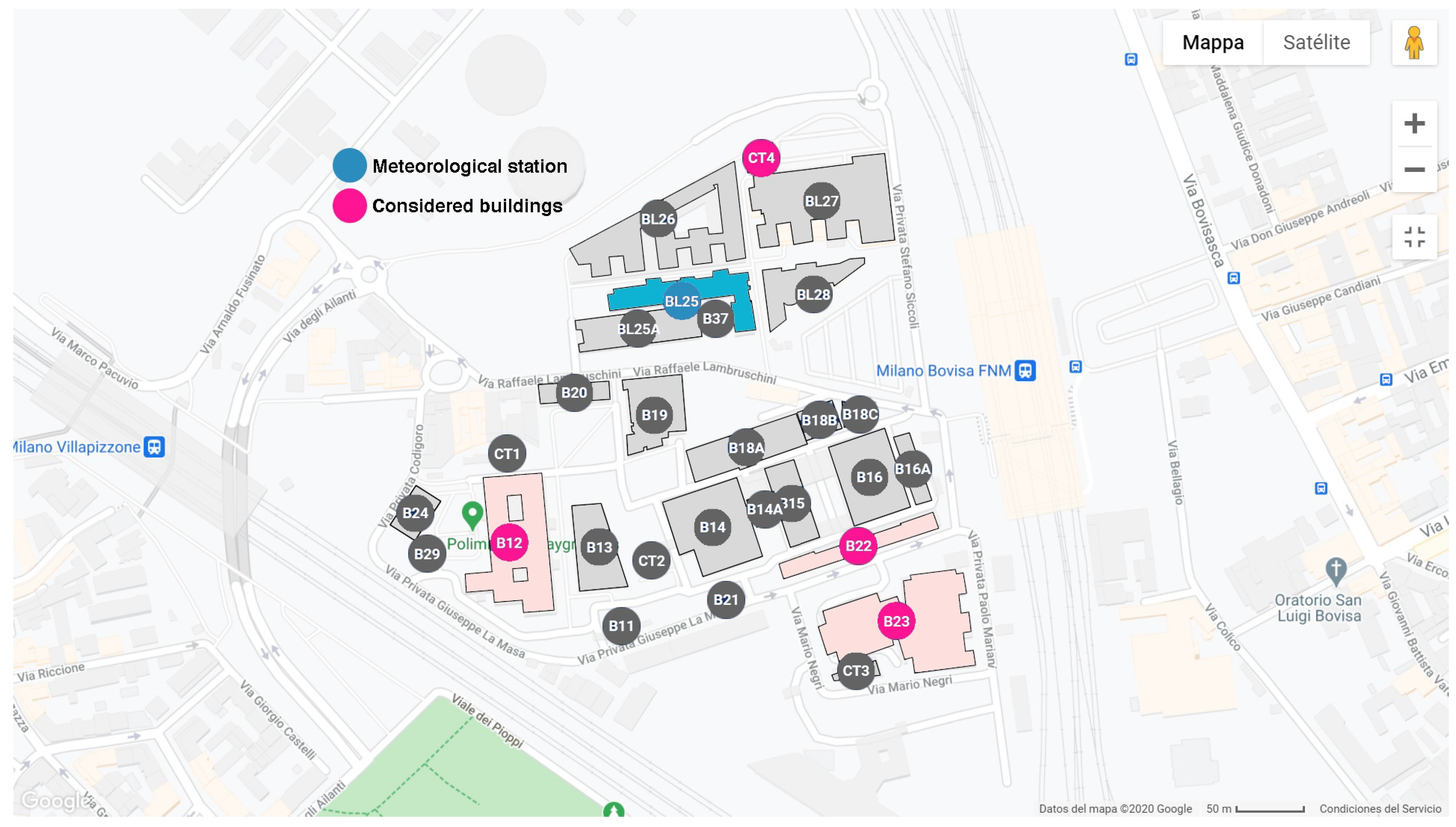
Section 2, the considered case study is presented. In
Section 3, the implemented steps to generate the probabilistic load forecast are illustrated.
Section 4 reports the discussion of obtained key results and, lastly, in
Section 5, the conclusions and final remarks are discussed.
3. Methods Implementation
To generate the probabilistic load forecasts, different steps were undertaken. One can visualize it as a five-stage process: the similar day method, where the data were preprocessed to find consumption phenotypes; nonparametric feature selection; point forecast through artificial neural networks; and, finally, a dynamical ensemble to generate the probabilistic load forecast. This section briefly describes the methods and their implementation.
3.1. Similar Day Method
Data are observations of real-world phenomena [
20]. They are the bridge between the model and the physical world [
21]. Preprocessing is imperative to improve models’ accuracy when representing reality, assuming the future will, somehow, look similar to the past. The approach taken in this work was to study the historical data to find the most representative patterns which underlined the hidden structures in the data. In biology, the term
phenotype refers to observable properties of an organism, which include appearance, development and behavior.
Some examples are wing length or hair color. In energy engineering, this term is adopted to describe the properties of daily consumption profiles [
22]. To find the consumption phenotypes, the load time series was transformed into strings by means of the Symbolic Aggregate ApproXimation (SAX) transformation [
23]. Like so, it was possible to take advantage of robust text mining techniques and classify the daily profiles into motifs and discords, which are the terms for frequent and infrequent patterns in data mining. The patterns with a frequency of less than 1% of the total available data were identified as discords and discarded. The motifs, on the other hand, were further aggregated into clusters by means of the k-means approach. By choosing the number of clusters
, the related profiles were identified as low-, medium- and high-consumption phenotypes.
3.2. Nonparametric Feature Selection
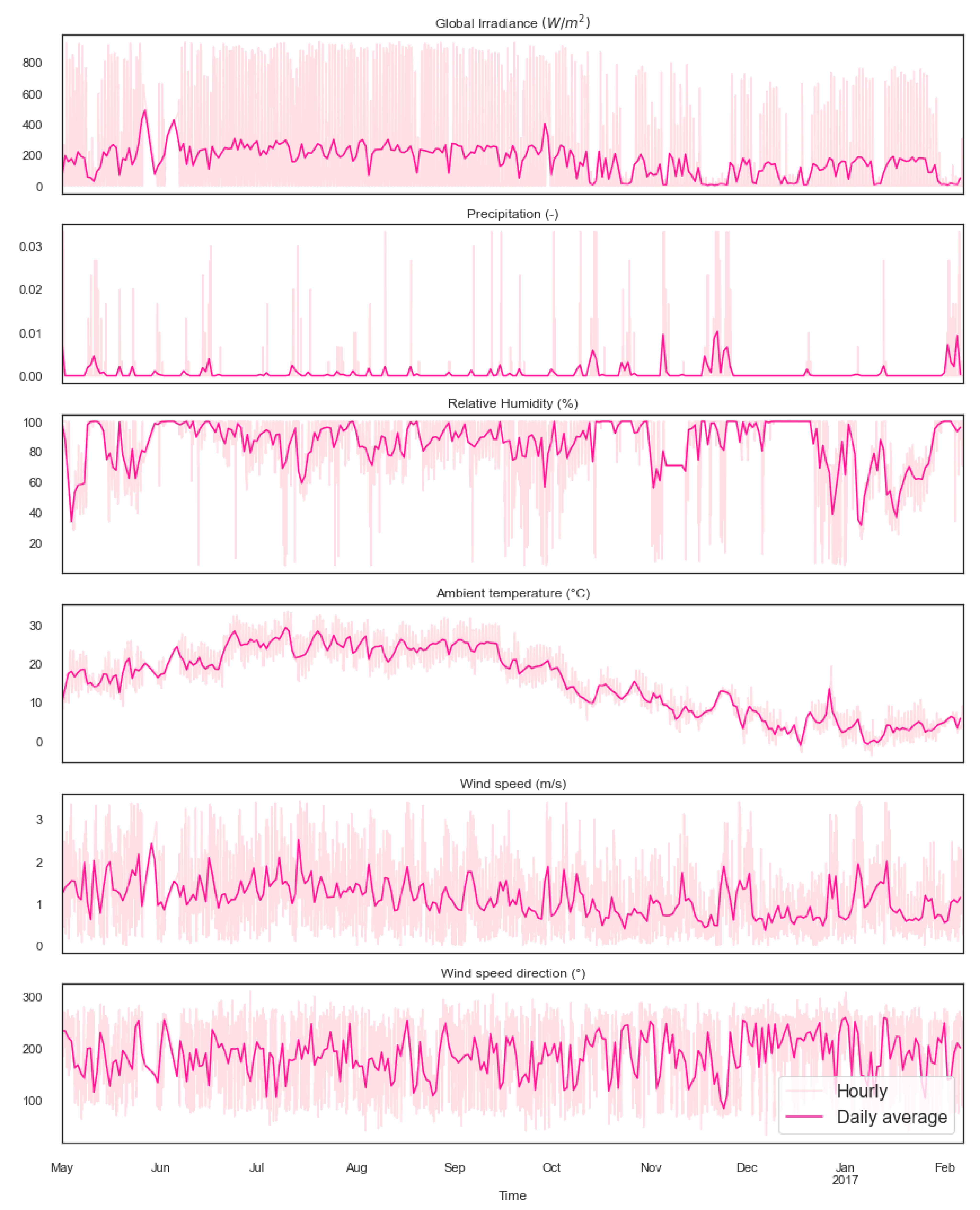
One of the research goals was to evaluate the importance of different effects as predictors of the load. Typically, in the literature, meteorological variables, particularly temperature, and load for the day before are employed.
Within the research framework, some other effects were explored, such as day–night and summer–winter shifts, together with the recency effect. The weather effects were enclosed by the hourly meteorological measurements. Day–night and seasonal shifts were captured by a cosine transformation of the respective hour and month indexes. The recency effect corresponds to a cognitive bias that makes people better remember the things said last in a speech. In the scope of energy demand, the recency effects explain the fact that electricity consumption is affected by temperatures of the preceding hours. This last effect is captured by the first and second derivatives of the meteorological variables.
The aforementioned effects were translated into a set of 43 candidate features. In order to select those with the greatest importance to predict the load and minimize the curse of dimensionality effects [
24], feature selection was undertaken. Mutual information (MI), which is a nonparametric approach, was applied. This kind of method provides details on the shared information among two variables. It is a measure of the uncertainty reduction of a target variable, while knowing the probability distribution function of another variable. The mutual information will be zero if, and only if, the two variables do not share any information at all. A feature subset of the ten highest MI variables was explored as input features on the artificial neural networks. Note that for all the cases, the highest MI was reported by the load for the day before, which indeed made a good predictor. However, it was left out of the models in order to avoid overfitting and to better appreciate the effects of adding the other predictors.
From all 43 candidates, models using from four up to ten of the most informative features were trained for each surveyed case. The symbols correspond to those listed in
Table 2:
L, the load;
, ambient temperature;
m, month index;
G, global solar irradiance;
h, hour index;
d, day index;
, relative humidity; and
, wind speed. For instance, the target day is denoted by
, whereas
indicates the day before. The first and second derivatives are denoted by
and
, respectively. For example, for predicting the hourly load
of the
d-th day for building CT4, the first most important input is the load of the day before
at the same hour
h; then, in the second place, the temperature on the target day
; then, in the third place, the temperature for the day before,
, at the same hour; and so on. Not surprisingly, the consumption and temperature of the day before come in the first places.
3.3. Point Forecast
The tagged consumption days were split into train, validation and test sets of sizes 80%, 10% and 10%, respectively. Ten different models based on artificial neural networks were proposed per phenotype.
Table 3 summarizes the models. M1 is a naive persistence model for the point forecasts, and M2 is used as a benchmark for the probabilistic forecasts. Note that the real measurements for the target day were used as proxy for an available temperature forecast. Additionally, when referring to a model trained for a specific phenotype, the subindexes
L,
M and
H were used to refer to low, medium or high consumption. For example,
would refer to
, trained, validated and tested on the high-consumption datasets.
All the models are feed-forward neural networks with back-propagation learning, specifically using the Adam optimizer with a learning rate equal to 0.001 [
25]. Each one had one hidden layer with rectified linear unit (ReLU) as the activation function between the input and hidden layer, and the linear transfer function (
) between the hidden and output layer. The batch size is equal to 48. The training and validation process was run 100 times. Additionally, the training was stopped if one of the following conditions was verified: (1) the number of epochs was greater than 500 or (2) the cost function was not improving for more than 10 consecutive epochs. For each model, the networks structure and the number of hidden neurons were found from employing the time series cross-validation line search, as depicted in [
26]. While this is not the most efficient way to fine-tune, it gives a sense of which direction to go; the results from this step are shown in
Table 4. The maximum number of neurons in the models for all the cases did not exceed 112, not even when 10 inputs were fed into the neuron. This raised the question on whether or not the feed-forward artificial neural networks were going to be able to fully capture complex relationships among the inputs.
The point forecast performance was assessed by means of the root mean squared error (RMSE) [
27], coefficient of variance of the root mean squared error (CVRMSE) [
28], enveloped mean absolute error (EMAE) [
29] and the well-known forecast skill (
S). Let us define the residual,
, given by the difference between an observed value
y and its forecast
, mathematically expressed as [
30]
Then, the aforementioned metrics are depicted as
where
N is the forecasts number,
is the mean of the test set load,
U is the uncertainty,
V is the variability of the load and RMSE
is the RMSE achieved by the persistence method. In particular, RMSE is widely used but has the drawback of being scale-dependent. Therefore, EMAE and CVRMSE were studied as well. Particular attention was paid to the latter, as the American Society of Heating, Refrigerating and Air-Conditioning Engineers (ASHRAE) defines as an acceptable accuracy a value of
for hourly predictions. Finally, the forecast skill score
S is often used to evaluate whether a model is superior compared with the naive method.
3.4. Probabilistic Load Forecast
In this work, to generate probabilistic load forecasts, a dynamical ensemble approach was adopted by considering a standard of 100 simulation runs for each considered model. These kinds of ensembles are obtained by evolving an ensemble of different initial conditions [
5]. Thus, the ensembles were constructed by adding perturbations on the original temperature profiles from the test set and making predictions with them. Herein, the perturbed scenarios were created by means of the truncated singular value decomposition (TSVD) [
31]. First, the temperature time series was recast into a matrix
, where
, and
d corresponds to the days the time series spans. Then, it was decomposed with the singular value decomposition into the product of three matrices:
where
and
are orthonormal unitary matrices, known as left and right singular matrices, respectively. The column vectors from
and
are known as the left and right singular vectors. Finally,
is a diagonal matrix, with the singular values on its diagonal, which correspond to the square root of the eigenvectors from the correlation matrix
.
By keeping only the leading singular values and the corresponding singular vectors to rebuild the time series with a low-rank approximation, the truncated singular value decomposition was adopted. Besides the first right singular vector, the rest were disturbed by means of Gaussian noise before going back to the time domain. Defining the standard deviation of the blended noise as , the added noise was gradually varied by varying from 0 to 0.2 in 0.01 increments. For each day of the test set, 100 scenarios were created. That way, temperature profiles were simulated for each day of the test day, allowing both to evaluate the uncertainty propagation into the point forecasts coming from faulty weather forecasts, to evolve the initial conditions of the analysis and, ultimately, create the dynamical ensembles.
After obtaining the different predictions, the percentiles from 1 to 99th were calculated and provided the prediction intervals for the probabilistic load forecast. The ANNs’ performance was assessed through pinball loss, a metric specifically designed for quantile forecasts [
6] and formulated as
where
is the point forecast for quantile
, and
y is the observation. They can be computed for each quantile and summed over the forecast horizon to attain the pinball loss. A low pinball loss score indicates an accurate probabilistic model.
4. Results
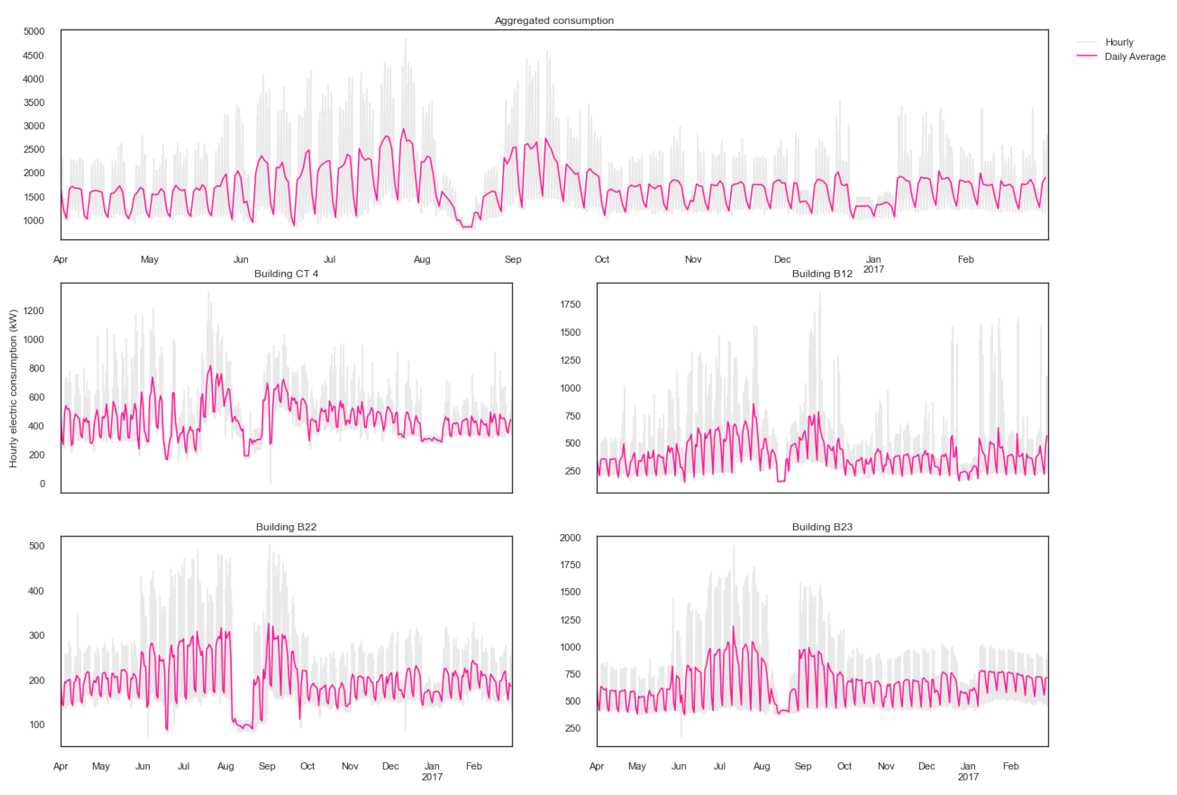
The aforementioned methods were implemented to forecast the electricity consumption for the day ahead of five different cases: four buildings and their aggregated consumption. Each case was studied separately, the main drivers and consumption phenotypes were identified per case, and ten models per phenotype were proposed. The mean performance from the 100 simulation run for the dataset was plotted.
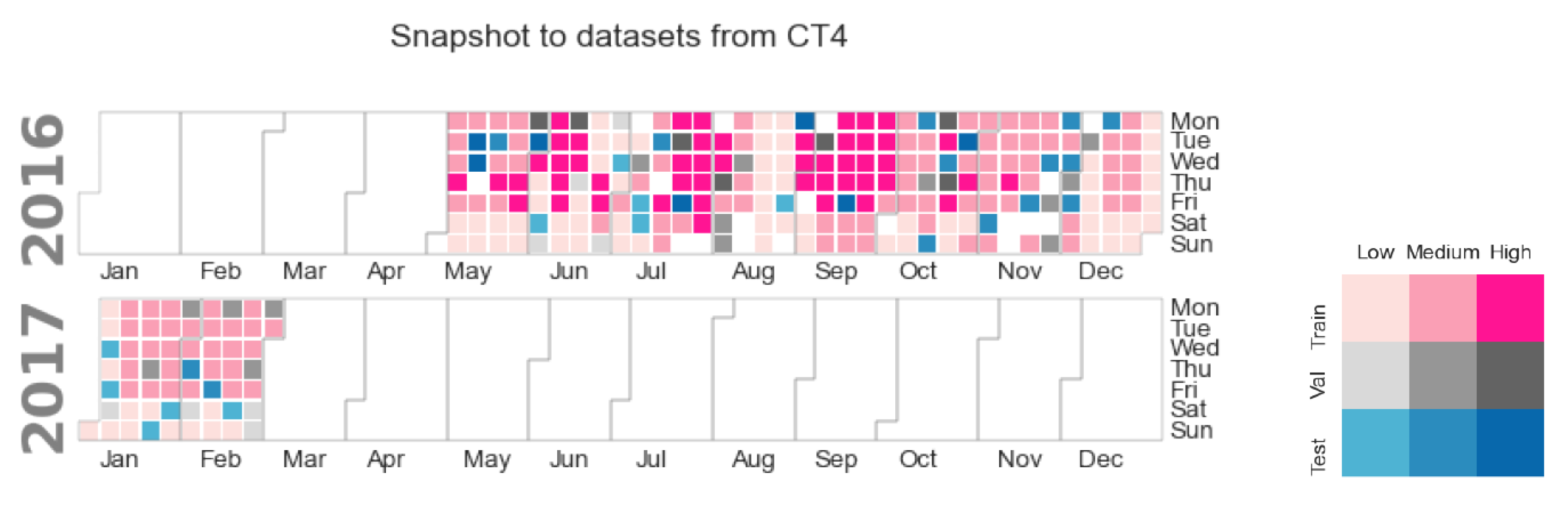
Figure 4 shows the datasets’ distribution along the time spanned for one of the studied buildings. The hue indicates consumption level: the darker the color, the higher the consumption. The pink shades depict training data; the validation days are in gray; and the test days are in blue. The figure allows us to observe that in the case of building CT4, low consumption levels coincide with weekends and holidays, and medium-level days are mostly in autumn and winter, thus in heating season, but also span weekends during the summer. However, the high-consumption days correspond mainly to working days in the cooling season. In fact, similar behaviors were found for the other studied cases.
Before proceeding, let us start by providing some notation used to refer to the input variables. The target day is denoted by d, while the day before corresponds to . The ambient temperature is depicted by ; G corresponds to the global solar radiation; refers to the relative humidity; L corresponds to the electric load; h to the hour; and m to the month. The first and second derivatives are depicted by ’ and ”, respectively. For example, would refer to the first derivative of the load from the day before.
The top ten features for each surveyed case suggest a strong dependency on seasonal effects, day–night shifts, solar heat gains through solar radiation, thermal inertia (particularly with
) and the recency effect through the first and/or second derivative of the solar radiation. Interestingly, for the oldest building among the studied cases, B12, the solar heat gains were more informative than temperature, after the hour of the day. In fact, by capturing these effects in most of the cases, the model’s accuracy was enough not only to outperform
and
but also to comply with ASHRAE’s benchmark and recent literature results with popular machine learning algorithms, such as RNN [
12,
19] and LSTM [
9].
The most accurate models on a CVRMSE basis are shown in
Table 5, highlighting their predictor variables. It can be observed that most of them received calendar variables, solar radiation for the target day and the day before, as well as their respective first and second derivatives. Considering the average accuracy of the best models per phenotype, it was somewhat surprising to find low and medium consumption to have similar accuracies, with CVRMSEs = 13.83% and 13.33%, respectively. The high-consumption models, on the other hand, were behind, with CVRMSE = 17.95%. It should be noted that there were more days tagged as medium than the other phenotypes. Thus, with more training examples, it should be possible to improve the results.
Specifically looking at each level,
was the most accurate among the proposed models, with an average CVRMSE = 12% for all the cases, as reported in
Table 6, which reports the average test performance of the ten models on the aggregated consumption of the four surveyed buildings.
This is a particularly relevant result if compared with popular machine learning algorithms, such as [
12,
19], where similar results have been obtained by means of an RNN on the same dataset, and it is better than [
9], where an LSTM approach resulted in a CVRMSE equal to 18.9%.
This indicates, indeed, that the best predictors for low-consumption days are calendar variables, such as day of the week, month of the year and hour of the day, but there is also little improvement compared with the naive benchmark. Since these days were mostly weekends and holidays, it may be worth to explore using dummy variables providing this information as predictors. In the case of medium- and high-consumption phenotypes, mainly
and
were the most accurate. As commented before, these models captured information on the weather, calendar variables, solar heat gains, thermal inertia and recency effects, suggesting a greater complexity to predict the demand, as more and diversified information was needed. To provide an example on the predicted values,
Figure 5 presents a test day from each consumption phenotype.
Through gradually perturbing the temperature profiles to generate predictions, the error propagation was studied. The results suggest that unless the temperature forecast completely missed the real conditions, the models’ performance was not significantly affected, thus maintaining similar accuracy to when real temperature measurements were employed for the load predictions. On the one hand, this may indicate the models to be robust to uncertainty from the weather forecast. On the other hand, it may also implicate low weights assigned to the temperature input; thus, exploring a different method to generate the prediction intervals should be considered.
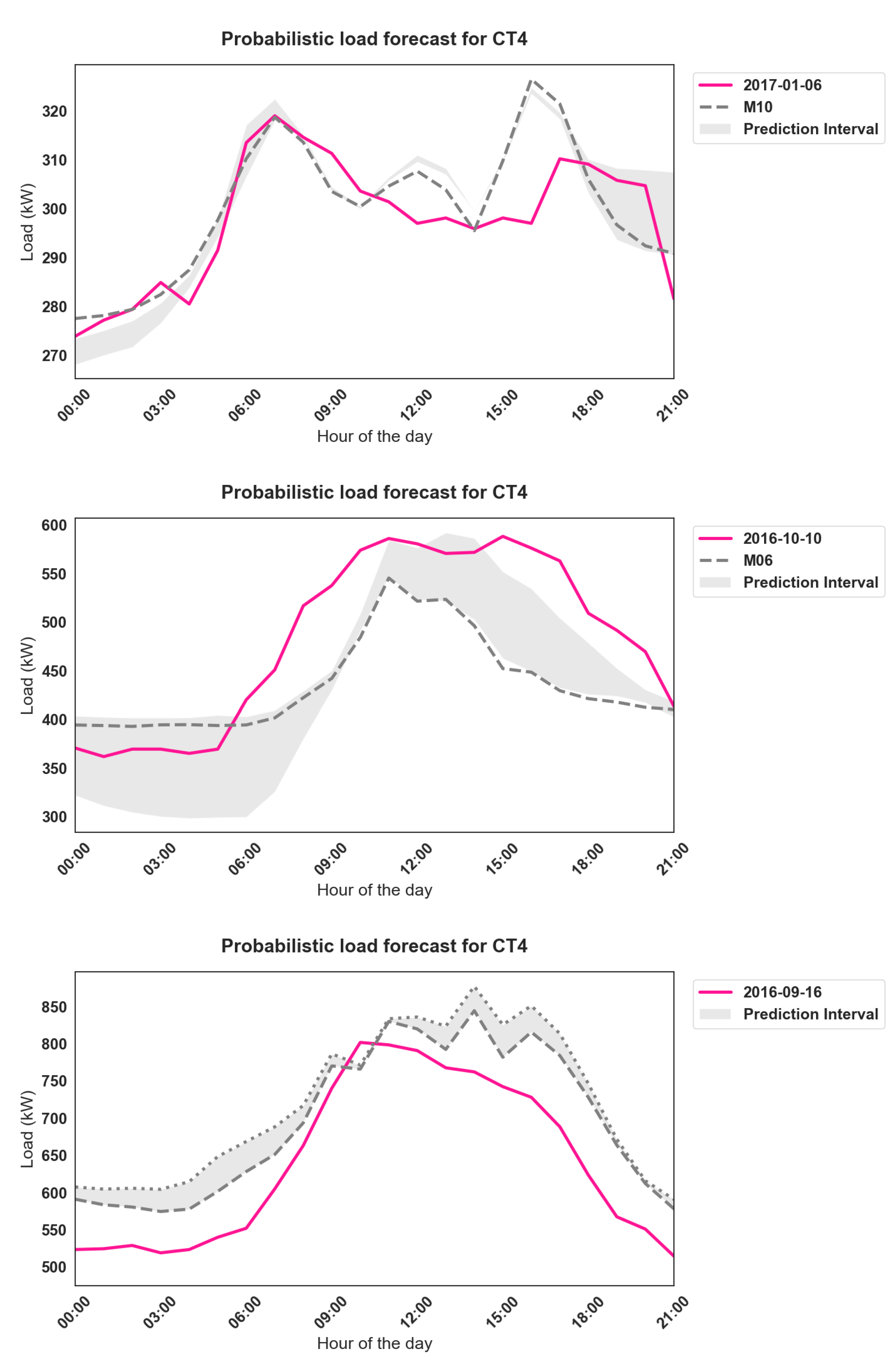
By adopting the dynamical ensemble approach, it was possible to generate prediction intervals, which better captured the true values compared with the point predictions.
Figure 6 presents an example of some of the generated probabilistic forecasts for a building among the studied cases.
From the pinball loss scores, an interesting result is remarked. Four out of five cases show the lowest loss for the low-consumption days, followed by medium and high last. Moreover, by adding information on the main drivers, the models outperformed—in most cases—the benchmark . In this case, however, the pinball loss cannot be readily comparable among the cases, as it is scale-dependent. After examining the results per phenotype, the following is commented. The low-consumption forecasts required simpler models than their medium- and high-consumption counterparts to achieve the lowest pinball loss. For instance, was among the best performing ones, adding only calendar variables to the ambient temperature. While for the other classifications, capturing additional details such as solar heat gains and recency effects was needed.
5. Conclusions
Five different cases of university buildings were studied. Point and probabilistic load forecasts for the day ahead were generated by means of feed-forward neural networks. In order to train the neural networks, the similar day method was adopted. The data available were classified into three daily consumption phenotypes, identified as low, medium and high. Ten models per phenotype were proposed and evaluated, two were used as benchmarks. Besides for the high-consumption models of one building, the rest not only outperformed the benchmark models but showed acceptable accuracies according to ASHRAE’s benchmark. A similar behavior was found from the probabilistic approach: providing information on different electricity consumption drivers, such as seasonal, day–night shifts and recency effects, improved the models’ performance against the benchmark. This indicates that using the most informative features indeed improved the predictions.
From the point forecast approach, some of the best results were from , which enclosed day–night and summer–winter shifts, thus highlighting the strong seasonal and opening hours dependency of the studied buildings, especially for weekends and holidays. However, working days tagged as medium- or high-consumption required more effects, such as heat gains and recency effects; indeed, models and were often times the most accurate.
Results from the error propagation analysis confirm the point forecasts to be robust to faulty weather forecast. Although employing a dynamical ensemble approach allowed to generate prediction intervals which better captured the true values in comparison with the point predictions, the calculated prediction intervals were too narrow, and overall, the considered approach did not provide useful prediction intervals. Since this method was applied unsuccessfully, it may be worth exploring a different approach to generate prediction intervals, such as fitting a probability density function on the residuals instead of the dynamic ensemble. Another option would be to generate scenarios based on solar heat gains rather than on temperature.
Finally, regarding future work, this research can be extended in multiple directions. The methodology was applied only for electric load, but provided there are available data, it could be employed for heat demand. Moreover, its application for different use types such as residential, commercial or industrial facilities could be explored. Furthermore, applying it within the smart cities paradigm and as a tool for energy communities could be viable as well. In fact, within the collective action approach, it could be possible to perform hierarchical forecasting, thus predicting the individual demand per unit and conforming the community to then forecast the aggregated consumption as a whole.

 ,
, 


