Article

Predicting the Oil Price Movement in Commodity Markets in Global Economic Meltdowns

Institute of Technology and Business in České Budějovice, School of Expertness and Valuation, Okružní 517/10, 37001 České Budějovice, Czech Republic
*
Author to whom correspondence should be addressed.
Forecasting 2023, 5(2), 374-389; https://doi.org/10.3390/forecast5020020
Submission received: 6 February 2023 / Revised: 22 March 2023 / Accepted: 23 March 2023 / Published: 27 March 2023
(This article belongs to the Section Forecasting in Economics and Management)

Abstract

:
The price of oil is nowadays a hot topic as it affects many areas of the world economy. The price of oil also plays an essential role in how the economic situation is currently developing (such as the COVID-19 pandemic, inflation and others) or the political situation in surrounding countries. The paper aims to predict the oil price movement in stock markets and to what extent the COVID-19 pandemic has affected stock markets. The experiment measures the price of oil from 2000 to 2022. Time-series-smoothing techniques for calculating the results involve multilayer perceptron (MLP) networks and radial basis function (RBF) neural networks. Statistica 13 software, version 13.0 forecasts the oil price movement. MLP networks deliver better performance than RBF networks and are applicable in practice. The results showed that the correlation coefficient values of all neural structures and data sets were higher than 0.973 in all cases, indicating only minimal differences between neural networks. Therefore, we must validate the prediction for the next 20 trading days. After the validation, the first neural network (10 MLP 1-18-1) closest to zero came out as the best. This network should be further trained on more data in the future, to refine the results.

1. Introduction

Oil prices require accurate predictions, given their imperativeness for the global economy [1]. Apart from fluctuating supply and demand, oil price movement reflects economic development, financial markets, conflicts, wars and political issues [2]. Vochozka et al. [3] argue that world oil prices spread into global economies, violently shaking macroeconomic dependent variables. Drebee and Razak [4] suggest that fluctuations in oil prices disrupt economic growth. Khan et al. [5] pointed out the beneficial influence of global crises and the COVID-19 pandemic when investors start to speculate about the possible commodity price volatility, while Dai et al. [6] showed dramatic oil price changes during emergencies.
Resource prices seriously harm the exchange rate [7]. Vochozka, Suler and Marousek [8] suggest that the EUR/USD rate strongly depends on oil values, reflecting shifts in supply and demand and global macroeconomic and geopolitical issues [9]. Supply and demand and the investors’ sentiment chiefly factor into oil price movement [10].
The mounting financial crisis has driven up oil and gas prices, indicating increases by dozens of percentage points compared with previous years. Gas prices have recently soared by dozens of crowns [11]. Many markets can readily adapt to rising costs but fail to conform when costs decrease [12]. Chen and Sun [13] revealed an asymmetry between gas prices in China and the global trend, indicating direct correspondence when the price soars but maladaptation in the event of a slump. Lv, Dong and Dong [14] found that oil prices more profoundly affect stock returns in the sector of new energy vehicles than in other clean industries.
Xu et al. [15] suggest that the rise in gas prices should not shortly exceed 20%, to ensure a stable consumer market. Valadkhani and Smyth [16] confirmed that while consumers feel a slow and steady drop in commodity prices, their perception of the opposite is delayed but more intensive.
The Czech Association of Petroleum Industry and Trade [17] predicts the highest demand for oil in the 2030s and 2040s.
Fahmy [18] points to the growing interest in clean energy, which has profoundly impacted its price compared with oil prices and technological shares. Liden et al. [19] and Wang et al. [20] revealed that excessive oil and gas extraction has seriously polluted the environment. Mohamued et al. [21] proved an inverse relationship between oil prices and gas emissions in oil-exporting and -importing countries. The oil and gas sector has seen a tremendous improvement in oil and gas recycling. Although oil field development is costly, well-planned and advanced low-cost strategies will go a long way [22].
The work aims to predict oil prices on stock markets, assessing the impact of the COVID-19 pandemic. Toward this aim, we formulated the following research questions:
RQ1: What will be the oil and gas prices on the commodity market in November 2022?
The global economies are always subject to change, intermittently experiencing financial crises (e.g., 1929, 2008) or worldwide epidemics such as the COVID-19 pandemic. The second research question focuses on measuring the pandemic’s impact on the price movements of the given resources.
RQ2: What was the impact of the COVID-19 pandemic on oil stock prices?
The article includes literary research with links to up-to-date scholarly literature, while the methods involve a regression analysis using neural networks evaluated in the Statistica program. The results contain our findings, a discussion of the research questions and a comparison of our results with those of other authors. The conclusion reviews the findings, giving practical recommendations.
The paper refers to a very current topic addressing companies, researchers and governments. Nowadays, the price of oil, and subsequently the price of gasoline, is a highly discussed topic, especially with regard to the ongoing energy crisis, the war in Ukraine and instability in the world’s financial markets. This article uses the method of artificial neural networks, which is becoming more and more important in all possible problem-solving applications across all disciplines. The article is also unique in that it includes an authentic validation of the predicted oil price results. After further training the most successful neural networks for prediction, the selected networks can be applied to this issue in practice. An extensive sample of historical data is also used, which should ensure the relevance of the research. We are convinced that the results of this article will not only be beneficial to the academic community but also serve as a basis for further follow-up research, whose aim is to produce the most accurate prediction of oil prices in world markets.

2. Literature Research

Oil price movement calls for an accurate prediction, as it profoundly affects global economies [23,24]. In the field of energetics, researches have long discussed unstable oil prices in the stock market [25,26]. Qazi [27] found that oil price growth, triggered by global economy reinvigoration, hugely impacts the sentiment in the stock market. Low stock volatility and rising oil prices arouse rising expectations of money flows, whereas high fluctuations make markets focus on the crippling effects of enormous input costs.
Singhal, Choudhary and Biswal [7] revealed that oil prices send unmistakable signals to monetary and fiscal policies, profoundly affecting stock markets and rates of exchange. We can predict the impacts of volatile oil prices on the EUR/USD exchange rate, improving corporate competitiveness in international markets [28]. Vrbka, Horák and Krulicky [29] explored the influence of oil price movement in the global market on Chinese currency by using neural networks. Although their results showed that fluctuating oil prices in stock markets somehow affect the CNY/USD exchange rate, they failed to gauge the extent.
Vochozka, Horák and Krulicky [28] used an innovative neural network, long short-term memory (LSTM), for predicting oil prices, combining the created neural network with the integrated LSTM to forecast Brent oil prices. Herrera et al. [30] applied the same technique to explain the prices of oil, coal and gas. The RMSE and MAPE approaches measure the models’ accuracy, including an M-DM test for detecting statistically significant differences. The results show that machine-learning methods hugely outplay traditional econometric procedures, precisely identifying breakeven points.
Khan et al. [5] used a dynamic simulation model for their experiment. They revealed that oil prices, the number of remittances and direct cross-border investments kickstart the stock market, whereas exchange rates have rather damaging effects. Zhao, Zhang and Wei [31] applied a recursive dynamic model of general equilibrium, exploring the impacts of rising and falling oil prices on investments and sectors of renewable energy resources. The authors found that rising oil prices may encourage investments in renewable energy, reduce the factual GNP and improve the environment, while the declining trend has had the opposite effect. Dabrowski et al. [32] used block-exogeneity panel vector autoregressive models to prove that shocks in oil prices and unsteady market trends seriously harm the respective economies of oil-exporting countries.
Denghani and Zangeneh [33] proposed an alternative method, including biogeographic optimization (BMMR-BBO), to estimate West Texas Intermediate’s oil prices, achieving better outcomes than those of other techniques. Kumeka, Uzoma-Nwosu and David Wayas [34] used Granger causality, revealing that exchange rates may even stimulate the market, unlike what happened before the COVID-19 pandemic. On the other hand, the impulse response functions (IRFs) showed that oil price shocks provoked negative responses in exchange rates only after the pandemic. Zafeirou et al. [35] found that high oil prices induced demand for agricultural products used for biodiesel and ethanol production, where energy and agricultural commodity markets closely interact.
The presented studies suggest an avid global interest in the discussed topic, including many articles and innovative methods. However, the best techniques have yet to come. Scholars have also measured how oil prices shook stock markets or affected the environment. Artificial neural networks involve the most applicable methods. We, therefore, use neural structures for predicting oil price movement in November 2022 (RQ1), while time series will be better at assessing whether the COVID-19 pandemic harmed or left intact the given commodity (RQ2).

3. Materials and Methods

We measure oil price movement from 2000 to 2022 and the associated emission limits and costs that companies incurred. Detecting the fuel prices at gas stations allows us to explore the driving forces behind the substantial fuel price rise, either out of necessity or out of a distributor’s tactics to exploit the situation.
We collected the data from the macrotrends.net website access of 2 October 2022, disclosing oil prices on every negotiated day. Our study involved Brent oil prices (WTI) measured in barrel units, comprising daily data from the New York Stock Exchange (NYSE). The stock market uses two indexes, namely the NYSE Composite, covering all negotiated stock, and the Dow Jones Industrial Average (DJIA), adopted by 30 prominent companies listed in stock markets in the US. The NYSE is open from 9:30 a.m. to 4.00 p.m. local time, i.e., from 3:00 p.m. to 10:00 p.m. in the Czech Republic. NYSE markets observe US holidays, during which the exchange is closed.
Figure 1 presents the data distribution in three diverse histograms covering the period from 1 August 2020 to 29 December 2022. The histogram in gray represents the distribution based on level data; the blue is based on the logarithmic series; and the logarithmic return series is in red. The predictions are based on three types (level, log, and log return), while only level 1 is presented in the results section. However, estimated predictions with log and log return series are available on request. As can be seen from Figure 1, the distribution of data improves by moving from level to log and from log to log return. The series has the same number of observations, 5706, but differs in outliers. Over 58 data points were missing, but this problem has been solved through data interpolation.
The descriptive statistics Table 1 in the Appendix shows the skewness, kurtosis, the Jarque–Bera test, the minimum, the maximum and the number of observations. As can be seen from the skewness, kurtosis and the Jarque–Bera test, our data do not hold a normal distribution. However, this is quite natural for a time series with a daily frequency.
We use Statistica 13 software from TIBECO for data handling, applying linear regression and neural networks. The linear analysis involves a sample including the following functions: linear, polynomial, logarithmic, exponential, weighted polynomial and polynomial negative exponential smoothing. First, we calculate the correlation coefficient, i.e., the dependence of oil and gas prices on time. Regression neural structures will allow for a 0.95% confidence interval, generating the multilayer perceptron (MLP) and radial basis function (RBF) networks. The calculations comprise 5805 data, where time is an independent variable and the commodity price a dependent variable. Figure 2 and Figure 3 illustrate the MLP and RBF neural networks.
The equation for an MPL neural structure is as follows [38]:
y ( x ) = σ ( i = 0 n w i x i )
The equation for an RBF neural structure is as follows [38]:
y ( x ) = e ( x c b ) 2
where x represents the input values, y is the output, c is the center, b is the width, x c is the distance calculated according to the Euclidean metric, x c b is the internal potential of the RBF unit, and w is the weight value.
The time series comprises three categories: testing, training and validation. The training class involves 70% of the data and generates neural structures, while the rest contain 15% in each. Both groups measure the reliability of the detected neural model. The calculation covers 1000 neural networks, preserving the top 10. The hidden layer of multilayer perceptron networks contains 2 to 20 neurons, whereas the hidden layer of the RFB includes 10 to 30 neurons, which is the outer limit. The hidden and output MLP layers combine linear, logistic, hyperbolic tangent, exponential and sinus functions, leaving other settings at their defaults (within automatic network creation tools). The method of least squares will be used to calculate the neural networks. The mesh generation will be terminated if there is no improvement, i.e., a decrease in the value of the square aggregate. Only those neuron structures whose respective squared aggregates of residuals are the lowest possible relative to the actual gold development will be preserved. The Broyden–Fletcher–Goldfarb–Shanno (BFGS) algorithm is also used. It is a local optimization algorithm that adapts machine-learning algorithms, such as the logistic regression algorithm. Delays in the time series will not be considered, because of the need for extensive calculations and the need to perform an additional experiment afterward. Table 2 presents relevant formulae.
The error function comprises the least squares, as follows:
E S O S = 1 2 N i = 1 N y i t i 2
where N represents the number of trained cases, yi predicts the target variable, and ti is the target variable of the ith case.
We create a neural network to answer RQ1, predicting the price for the following month. The validation covers 20 consecutive trading days, including time series for exploring the existing and predicted values within the period. Answering RQ1 determines whether the oil price movement depends on economic development. The validation reveals the difference (residuals) between the evident price and the forecast price, indicating the top network to implement in practice. The best structure is always the one with predicted and existing values close to zero.
RQ2 covers the time series from 2000 to 2022, assessing whether the COVID-19 pandemic harmed commodity price movement. We include 5805 values, calculating the arithmetic mean for creating the time series by using a mean function in Excel. The mode and median function in Excel provide median and mean values. The minimum and maximum oil prices and dispersion measure the distance between the points. We use milestones during the COVID-19 pandemic, including the onset, growth and repercussions such as lockdowns. A graph illustrates the detected correlations between these events and oil price movement, providing calculations and visualizations of the findings.

4. Results

Table 3 presents the top 10 neural networks from 1000 generated structures.
All preserved networks are MLPs, largely outplaying the underperforming and biased RBFs. The top 10 structures contained 13 to 20 neurons in the hidden layer and were generated by the variant BFGS (Broyden–Fletcher–Goldfarb–Shanno) training algorithm. A hyperbolic tangent and logistic sigmoid activated hidden neural layers, whereas five functions initiated the output, including sine, identity, exponential, hyperbolic tangent and logistic. Table 4 illustrates the correlation coefficient determining the performance of the preserved structures in all the data sets.
The correlation coefficient should equal 1 when looking for the corresponding network. All three data sets performed the same, indicating valid structures in the training group, validated by the other two sets. Neural networks must show a minimum error rate in all three groups. According to Table 4,the correlation coefficients of all the neural structures and data sets exceed 0.973, suggesting minimal differences between the networks. Table 5 then presents the statistical analysis for predictions.
Table 4 presents the prediction statistics with residuals. They should be close to zero, indicating corresponding values of the input and predicted data. We can also see some residuals in these networks, containing slight inaccuracies. Figure 4 depicts all the networks and the actual price movement, including these values. We provide only a part of the table, enclosing the rest in the attachments. Figure 4 demonstrates oil price movement.
The figure proposes that all neural networks performed reasonably well in tracking actual oil price movement. Colored curves represent 10 preserved structures, yet they cannot indicate the local minimum and maximum variations. Even though the networks have very high performance levels, according to the correlation coefficients, they encounter a problem when predicting price fluctuations (lowest and highest points). For example, the value of 2100 skyrocketed. This is because the global financial crisis started in 2008, and the price of oil rapidly rose. The value in a horizontal axis (case number) is expressed by the number of observations (detailed input data, in days). Within a few years, the price of oil again sharply fell as the financial crisis was still lingering, and there was not as much money to trade in oil. It can be seen that from the value of 2400, the price of oil rose to the value of 2800, where it stagnated until it reached a value of 3700, where again the price of oil rose to the value of 4100 and then rose again until it reached a value of 5200. At this point, oil prices hit a trough without networks’ noticing the slump. This case marks the onset of the COVID-19 pandemic, witnessing a global social and business lockdown. However, why none of the networks could track the alarming situation remains a mystery. Despite this inconvenience, all the networks are applicable in practice. In 2022, the price of oil again sharply rose, because in February 2022, war broke out in Ukraine. Except for the fluctuation at the value of 5200, when the neural networks could not record this extreme, the neural network more successfully captured the last changes. After training the neural structures, we predicted oil price movement for 20 consecutive days, depicted in Table 6.
Table 6 depicts oil price movement from 8 November 2022 to 5 December 2022. The first two networks show a price range from 91.75 to 95.15. On the other hand, from the third structure, we see an inconsistent rise and fall. Strangely enough, the sixth and eighth networks mark price hikes in November, while the seventh model indicates a slump below the level of other neural networks, which do not drop under 81.42. Table 7 illustrates actual oil price movement for November 2022.
We can see that the actual oil price was much lower than what some neural networks predicted. At the beginning of November, the price topped USD 96.85 per barrel, witnessing a steady decline until 30 November 2022. At that time, the values again increased until 5 December and then plummeted to the rates before 30 November.
Table 8 presents the differences between real oil prices and predictions of oil prices.
We can see that the first neural network, whose total value, mean and median are the closest to zero, closely mimicking reality, shows the best results. On the other hand, the sixth neural network performed the worst, indicating the highest dispersion, forecasting much higher oil prices. The seventh neural structure did not perform well, either, setting the price too low compared to the actual situation. Table 8 also shows that the predicted price was close to reality on the 8th, 11th and 15th of November. Most residuals are minus, demonstrating huge differences between the predicted data and the actual data. This issue can also be looked at in the form of trend monitoring. Although some prediction networks showed very different values from the actual value, they successfully followed the trend of natural development (more or less similar decline and growth). This can be seen, for example, in the seventh MLP 1-17-1 network if we compare the predicted values, in Table 6, and the actual values, in Table 7.
Figure 5 illustrates the price difference between gasoline and oil.
The extreme variations indicate that oil prices wildly fluctuated during the monitored period compared with gasoline prices. Figure 5 proposes that 2008 and 2009 saw a price hike after the Great Recession, followed by a sharp drop in 2009. Despite the ongoing financial crisis, global markets found a way to push oil prices up again, as shown in Figure 5. The next economic upheaval came in 2020, when the COVID-19 pandemic inhibited the global economy with massive lockdowns until 2021. It can be seen from Figure 5 that there was a massive drop in the price of oil at this time: before the onset of the COVID-19 pandemic, the cost of oil hovered around USD 63 per barrel, and at the beginning of the pandemic (i.e., sometime around 1 January 2020), the price of oil fell only slightly, to USD 59 per barrel. The big jump happened around 22 July 2020, when the price of oil had fallen to USD 9 per barrel. As of August 2020, the cost of oil again started to rise. In 2022, the war in Ukraine again dramatically drove oil prices up, yet leaving gasoline prices intact. What causes the wild fluctuation of fuels? Gasoline reflects oil prices, including high taxes (excise duty and GNP) and refinery margins that increase the limit 10 times during a crisis. The Russia–Ukraine War also contributes to high fuel prices, because the US and the EU banned oil imports from Russia, relying heavily on shippers from other countries.

5. Discussion

This work explored oil price movement in stock markets and the extent that they suffered from the COVID-19 pandemic. The data analysis covered the years 2000 to 2022, including 5805 items processed in Statistica 13 software. Recent years have seen much research on commodity price movement, using artificial neural networks calculated in Statistica and Matlab. Vochozka, Horák and Krulicky [28] listed the most common software tools, including JavaScript, Python, Tensor Flow and Matlab.
Naderi, Khamehchi and Karimi [40] applied neural structures to predict monthly oil prices, daily gas prices and annual interest rates. Their findings revealed that their method reduces the mean squared error by at least 6.61% in the monthly oil price, 18.33% in the daily gas price and 23.13% in the annual interest rate prognosis compared with other forecasting techniques.
The research questions of this study were as follows:
RQ1: What will be the oil and gas prices on the commodity market in November 2022?
Answering RQ1 involved a neural network predicting commodity prices for the following month, revealing that November 2022 saw oil prices between USD 91.75 and USD 125.48 per barrel. The first two neural structures showed price movement between USD 91.75 and USD 95.15, while the values of the rest fluctuated. Strangely enough, the sixth and eighth networks indicated a sharp price hike during November, while the seventh network indicated much lower values than the other neural networks, which never dropped below USD 81.42. The oil price will then be on the rise. We generated 1000 neural models, preserving the top 10. All of them were MLP models, including 13–20 neurons in the hidden layer and trained by variants of the BFGS (Broyden–Fletcher–Goldfarb–Shanno) algorithm. The correlation coefficients of all the networks and data sets were higher than 0.973, showing only minimal differences.
RQ2: What was the impact of the COVID-19 pandemic on oil stock prices?
RQ2 comprised a time series from 2000 to 2022, measuring the impact of the COVID-19 pandemic on oil price movement and a potential slump in commodity prices. We found that the pandemic was the main driving force behind the oil rates. Although the onset did not damage the market much, consequent lockdowns severely inhibited the economy, driving oil prices down. The rates did not begin to rise until 2021.
We also explored fuel prices at petrol stations, assessing whether they were due to inflation or to distributors’ seizing the opportunity to boost profits. Because oil prices have incurred violent fluctuations over the past two decades while gasoline has commanded the same market price, it is evident that distributors only seized an opportunity in the calamity. The gas reflects oil rates, including high taxes (excise duty and GNP), and refinery margins increased 10 times when expecting or experiencing a crisis. Another contributor to exorbitant fuel prices is the ongoing war in Ukraine, as the US and the EU banned oil imports from Russia, looking for supplies from elsewhere.

6. Conclusions

Predicting commodity prices is essential for developing effective strategies for efficiently handling stock market transactions. All the people involved in the stock exchange follow forecasts of price movements, including shareholders, traders and companies. Oil prices also draw in the public, as this resource concerns our daily lives. Predicting commodity prices is essential for developing effective strategies for efficiently handling stock market transactions. All the people involved in the stock exchange follow forecasts of price movements, including shareholders, traders and companies.
The present study aimed to predict oil price movement in stock markets, assessing the impact of the COVID-19 pandemic. We found that oil deeply upset gasoline prices, closely reflecting the economic (the pandemic, inflation) or political situation in neighboring countries.
If Europe or the world faces a war or a pandemic, commodity prices (oil) soar, and they are highly susceptible to supply and demand and deeply suffer from economic plights. The correlation coefficients of all the neural networks and data sets exceeded 0.973, indicating only minimal differences. Another partial goal was to find out the price at which fuel is sold at gas stations and assess whether it is necessary to raise the price or whether it is a classic move by distributors to use the situation to their advantage and increase profits. It was found that this is a classic move by distributors, as the price of benzene has hardly moved over the past 20 years, while the price of oil, on the other hand, has had a very fluctuating tendency. However, we also have to consider that tax is included in the price of gasoline, and the margin of refineries is also included here, which can increase this margin even 10 times when a crisis period is expected or a crisis period is currently underway. Another reason fuel prices are so high now is the ongoing war in Ukraine, as the US and the EU have banned the oil supply from Russia, so there is pressure on the oil supply from other countries.
We also revealed that all neural networks performed well in tracking actual oil price movement, although some undetected fluctuations occurred over the monitored period. Despite these setbacks, all the models are applicable in practice. Once trained, the networks predicted oil price movement for 20 trading days. The total correlation coefficients showed that the 10th MLP 1-18-1 network was the best to apply in practice. The seventh neural network was the best at predicting the trend following the development of the actual value, but the residual was the worst. The residual at the seventh neural network came out USD 20 lower, but it managed the trend the best despite that.
However, the coefficients are so close, almost identical, that we cannot satisfactorily say which network is the best. All the networks need further training to yield results that are more accurate. Validation showed that the first model was closest to zero and, thereby, the most reliable to train on extensive data to achieve higher accuracy. Although all the networks can somehow predict oil price movement, they are still too far from reality to be suitable in practice.
Oil prices were calculated using the least squares method. Time series lags were not considered, because of because of the need for extensive calculations and the need to perform additional experiments afterward. This should be the subject of ongoing research. According to the correlation coefficients, the networks are of high quality and perform well, but when the residuals are added up, it is found that they are not so good, as the networks can smooth the historical time series of oil prices very well but are less useful at providing accurate predictions, especially for a more-extended period.
The study is limited by involving only a few neural networks. Our research also lacked a comparison with other commodities, as we explored only oil prices. The survey will continue by validating the oil price for December 2022. Furthermore, it would be helpful to solve another analysis on the development of the trend in noniron networks because, in most cases, they cannot have the same values as the residuals can. Neural networks cannot capture local minima and maxima but can detect a trend. They also cannot capture extremes, as they are preset, so it is necessary to take the structures of these preserved networks, train them on new ones and improve their predictive abilities.

Author Contributions

Conceptualization, J.H. and M.J.; methodology, J.H. and M.J.; software, J.H. and M.J.; validation, J.H.; formal analysis, M.J.; investigation, J.H.; resources, M.J.; data curation, J.H. and M.J.; writing—original draft preparation, M.J.; writing—review and editing, J.H.; visualization, M.J.; supervision, J.H. All authors have read and agreed to the published version of the manuscript.

Funding

This research was supported/funded by IVSUZO2301—The impact of the circular economy on the share prices of companies listed on the stock exchange.

Institutional Review Board Statement

Not applicable.

Informed Consent Statement

Not applicable.

Data Availability Statement

The data sets used in this contribution were sourced from https://www.macrotrends.net/2480/brent-crude-oil-prices-10-year-daily-chart (accessed on 25 November 2022).

Conflicts of Interest

The authors declare no conflict of interest.

References

  1. Zhao, L.T.; Wang, Z.J.; Wang, S.P.; He, L.Y. Predicting Oil Prices: An Analysis of Oil Price Volatility Cycle and Financial Markets. Emerg. Mark. Financ. Trade 2021, 57, 1068–1087. [Google Scholar] [CrossRef]
  2. Liu, J.; Huang, X. Forecasting Crude Oil Price Using Event Extraction. IEEE Access 2021, 9, 149067–149076. [Google Scholar] [CrossRef]
  3. Vochozka, M.; Horak, J.; Krulicky, T.; Pardal, P. Predicting future Brent oil price on global markets. Acta Montan. Slovaca 2020, 25, 375–392. [Google Scholar]
  4. Drebee, H.A.; Razak, N.A.A. Impact of Oil Price Fluctuations on Economic Growth, Financial Development, and Exchange Rate in Iraq: Econometric Approach. Ind. Eng. Manag. Syst. 2022, 21, 110–118. [Google Scholar] [CrossRef]
  5. Khan, M.I.; Teng, Z.; Khan, M.K.; Khan, M.F. The impact of oil prices on stock market development in Pakistan: Evidence with a novel dynamic simulated ARDL approach. Resour. Policy 2021, 70, 101899. [Google Scholar] [CrossRef]
  6. Dai, W.; Pan, W.; Shi, Y.; Hu, C.; Pan, W.; Huang, G.E. Crude Oil Price Fluctuation Analysis Under Considering Emergency and Network Search Data. Global Chall. 2020, 4, 2000051. [Google Scholar] [CrossRef]
  7. Singhal, S.; Choudhary, S.; Biswal, P. Return and volatility linkages among international crude oil price, gold price, exchange rate, and stock markets: Evidence from Mexico. Resour. Policy 2019, 60, 255–261. [Google Scholar] [CrossRef]
  8. Vochozka, M.; Suler, P.; Marousek, J. The influence of the international price of oil on the value of the EUR/USD exchange rate. J. Compet. 2020, 12, 167–190. [Google Scholar] [CrossRef]
  9. Demirbas, A.; Al-Sasi, B.O.; Nizami, A.S. Recent volatility in the price of crude oil. Energy Sources Part B Econ. Plan. Policy 2017, 12, 408–414. [Google Scholar]
  10. Zheng, Y.H.; Du, Z. A systematic review in crude oil markets: Embarking on the oil price. Green Financ. 2019, 1, 328–345. [Google Scholar] [CrossRef]
  11. Glaserova, D. Ceny Benzinu Stále Rostou, Klesají Naopak u Nafty. Nejdramatičtější je Vývoj u Alternativních Paliv [The Prices of Gasoline Are Still Rising, Diesel Prices Are Declining. The Development of Alternative Fuels Is the Most Dramatic]; Czech Television: Prague, Czech Republic, 2022. [Google Scholar]
  12. Byrne, D.P. Gasoline Pricing in the Country and the City. Rev. Ind. Organ. 2019, 552, 209–235. [Google Scholar]
  13. Chen, H.; Sun, Z. International crude oil price, regulation and asymmetric response of China’s gasoline price. Energy Econ. 2021, 94, 105049. [Google Scholar] [CrossRef]
  14. Lv, X.; Dong, X.; Dong, W. Oil Prices and Stock Prices of Clean Energy: New Evidence from Chinese Sub-sectoral Data. Emerg. Mark. Financ. Trade 2019, 57, 1088–1102. [Google Scholar]
  15. Xu, L.; Chen, F.; Qu, F.; Wang, J.; Lu, Y. Queuing to refuel before price rise in China: How do gasoline price changes affect consumer responses and behaviours? Energy 2022, 253, 124166. [Google Scholar] [CrossRef]
  16. Valadkhani, A.; Smyth, R. Asymmetric responses in the timing, and magnitude, of changes in Australian monthly petrol prices to daily oil price changes. Energy Econ. 2018, 69, 89–100. [Google Scholar]
  17. The Czech Association of Petroleum Industry and Trade. Ropa Jako Nenahraditelná Surovina [Oil as an Irreplaceable Raw Material]. 2021. Available online: https://www.cappo.cz/pohonne-hmoty-a-energie-pro-mobilitu/ropa-jako-nenahraditelna-surovina (accessed on 11 November 2022).
  18. Fahmy, H. The rise in investors’ awareness of climate risks after the Paris Agreement and the clean energy-oil-technology prices nexus. Energy Econ. 2022, 106, 105738. [Google Scholar] [CrossRef]
  19. Liden, T.; Santos, I.C.; Hildenbrand, Z.L.; Schug, K.A. Treatment modalities for the reuse of produced waste from oil and gas development. Sci. Total Environ. 2018, 643, 107–118. [Google Scholar] [CrossRef]
  20. Wang, J.; Li, X.; Hong, T.; Wang, S. A semi-heterogeneous approach to combining crude oil price forecasts. Inf. Sci. 2018, 460, 279–292. [Google Scholar] [CrossRef]
  21. Mohamued, E.A.; Ahmed, M.; Pyplacz, P.; Liczmanska-Kopcewicz, K.; Khan, M.A. Global Oil Price and Innovation for Sustainability: The Impact of R&D Spending, Oil Price and Oil Price Volatility on GHG Emissions. Energies 2021, 14, 1757. [Google Scholar]
  22. Song, X.; Qu, D.; Zou, C. Low-cost development strategy for oilfields in China under low oil prices. Pet. Explor. Dev. 2021, 48, 1007–1018. [Google Scholar] [CrossRef]
  23. Wang, C.; Lü, Y.; Song, C.; Zhang, D.; Rong, F.; He, L. Separation of emulsified crude oil from produced water by gas flotation: A review. Sci. Total Environ. 2022, 845, 157304. [Google Scholar] [PubMed]
  24. Li, X.; Ventura, J.A.; Ayala, L.F. Carbon dioxide source selection and supply planning for fracking operations in shale gas and oil wells. J. Nat. Gas Sci. Eng. 2018, 55, 74–88. [Google Scholar] [CrossRef]
  25. Ge, Y.; Wu, H. Environmental Assessment of Asymmetric Hysteresis of China’s Crude Oil Price to Gasoline Price. Ekoloji 2018, 27, 1563–1574. [Google Scholar]
  26. Shahid, I.; Siddique, A.; Nawas, T.; Tahir, M.B.; Fatima, J.; Hussain, A.; Alrobei, H. Heterogeneous nanocatalyst for biodiesel fuel production: Bench scale from waste oil sources. Z. Fur Phys. Chem. Int. J. Res. Phys. Chem. Chem. Phys. 2022, 236, 1377–1410. [Google Scholar] [CrossRef]
  27. Qazi, U.Y. Future of Hydrogen as an Alternative Fuel for Next-Generation Industrial Applications; Challenges and Expected Opportunities. Energies 2022, 15, 4741. [Google Scholar]
  28. Vochozka, M.; Horak, J.; Krulicky, T. Innovations in management forecast: Time development of stock prices with neural networks. Mark. Manag. Innov. 2020, 2, 324–339. [Google Scholar]
  29. Vrbka, J.; Horak, J.; Krulicky, T. The Influence of World Oil Prices on the Chinese Yuan Exchange Rate. Entrep. Sustain. Issues 2022, 9, 439–462. [Google Scholar]
  30. Herrera, G.P.; Herrera, G.P.; Constantino, M.; Tabak, B.M.; Pistori, H.; Su, J.J.; Naranpanawa, A. Long-term Forecast of Energy Commodities Price Using Machine Learning. Energy 2019, 179, 214–221. [Google Scholar]
  31. Zhao, Y.; Zhang, Y.; Wei, W. Quantifying International Oil Price Shocks on Renewable Energy Development in China. Appl. Econ. 2020, 53, 329–344. [Google Scholar]
  32. Dabrowski, M.A.; Papiez, M.; Rubaszek, M.; Smiech, S. The Role of Economic Development for the Effect of Oil Market Shocks on Oil-Exporting Countries: Evidence from the Interacted Panel VAR Model. Energy Econ. 2022, 110, 106017. [Google Scholar] [CrossRef]
  33. Dehghani, H.; Zangeneh, M. Crude Oil Price Forecasting: A Biogeography-Based Optimization Approach. Energy Sources Part B Econ. Plan. Policy 2018, 13, 328–339. [Google Scholar]
  34. Kumeka, T.T.; Uzoma-Nwosu, D.C.; David-Wayas, M.O. The Effects of COVID-19 on the Interrelationship Among Oil Prices, Stock Prices and Exchange Rates in Selected Oil Exporting Economies. Resour. Policy 2022, 77, 102744. [Google Scholar] [CrossRef] [PubMed]
  35. Zafeiriou, E.; Arabatzis, G.; Karanikola, P.; Tampakis, S.; Tsiantikoudis, S. Agricultural Commodities and Crude Oil Prices: An Empirical Investigation. Sustainability 2018, 10, 1199. [Google Scholar] [CrossRef] [Green Version]
  36. Keim, R. How to Train a Multilayer Perceptron Neural Network. All About Circuits 2019. Available online: https://www.allaboutcircuits.com/technical-articles/how-to-train-a-multilayer-perceptron-neural-network/ (accessed on 11 November 2022).
  37. He, H.; Yan, Y.; Chen, T.; Cheng, P. Tree Height Estimation of Forest Plantation in Mountainous Terrain from Bare-Earth Points Using a DoG-Coupled Radial Basis Function Neural Network. Remote Sens. 2019, 11, 1271. [Google Scholar]
  38. Kudova, P. Neuronové Sítě Typu RBF pro Analýzu dat [BF Type Neural Networks for Data Analysis]. Master’s thesis, Charles University, Prague, Czech Republic, 2001. [Google Scholar]
  39. Suler, P.; Machova, V. Better Results of Artificial Neural Networks in Predicting ČEZ Share Prices. J. Int. Stud. 2020, 13, 259–278. [Google Scholar] [CrossRef]
  40. Naderi, M.; Khamehchi, E.; Karimi, B. Novel statistical forecasting models for crude oil price, gas price, and interest rate based on meta-heuristic bat algorithm. J. Pet. Sci. Eng. 2019, 172, 13–22. [Google Scholar]
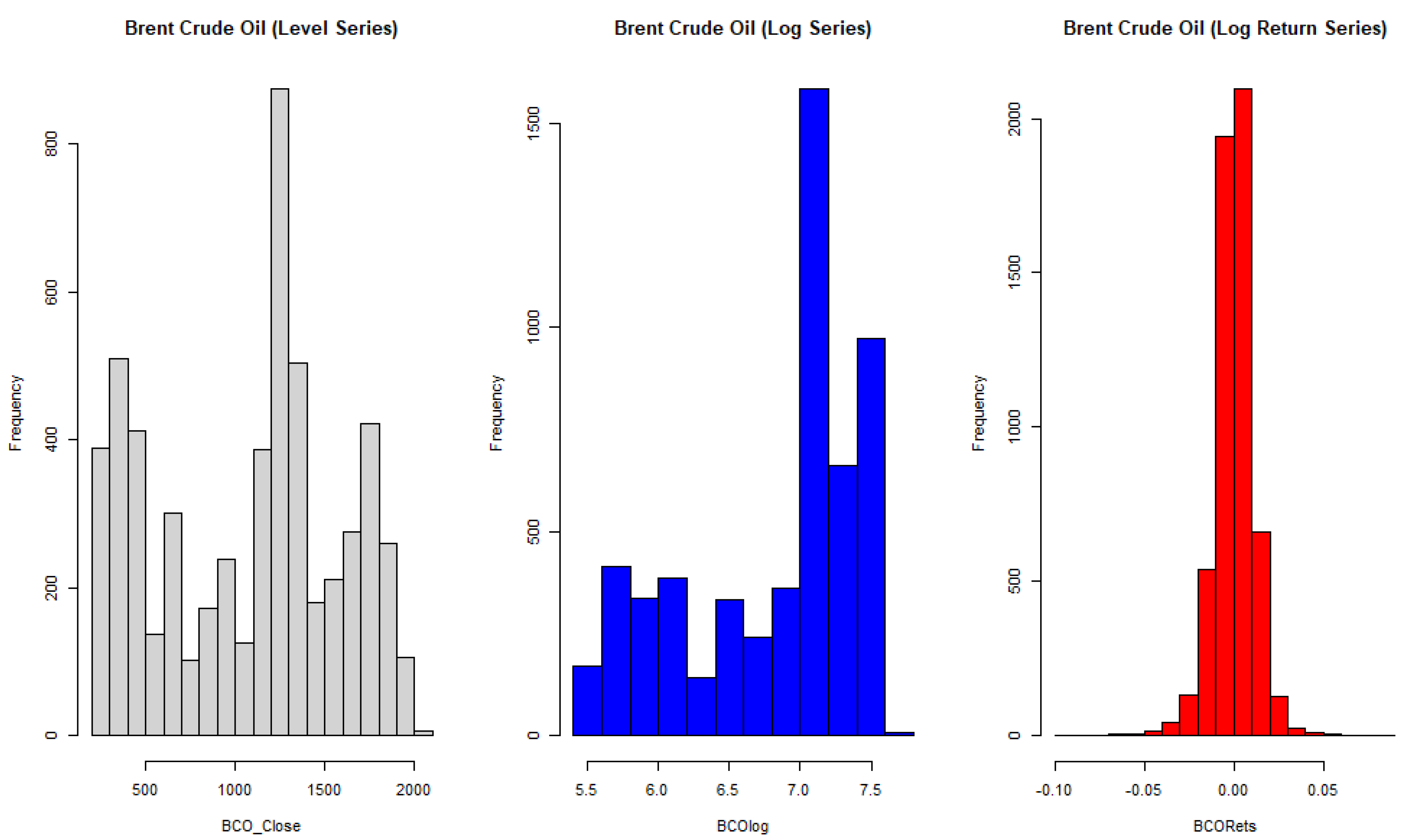
Figure 1. Histogram distribution with level, log, and log return series. Source: authors’ elaboration, based on R studio.
Forecasting 05 00020 g001
Figure 2. MLP neural networks. Source: [36].
Forecasting 05 00020 g002
Figure 3. RBF neural networks. Source: [37].
Forecasting 05 00020 g003
Figure 4. Oil price movement. Source: authors.
Forecasting 05 00020 g004
Figure 5. Price differences between oil and gasoline. Source: authors.
Forecasting 05 00020 g005
Table 1. Descriptive statistics, based on level, log and log return series.
TypenMeanMedianStdSkewKurtosisMinMaxJB
BCO (Level)56071070.81204.3511.37−0.15−1.21255.120510.000
BCO (Log)56076.827.090.61−0.74−0.845.547.630.000
BCO (Log
Return)
56070.000.000.010.295.42−0.10.090.000
Source: authors.
Table 2. Activation function of hidden and output layers of MLP and RBF.
FunctionDefinitionRange
Identitya , +
Logistic sigmoid 1 1 + e a (0, 1)
Hyperbolic tangent e a e a e a + e a (−1, +1)
Exponential e a 0 , +
Sine sin   a 0 ,   1
Source: [39].
Table 3. Summary of active networks (oil—daily data from 2000 to 2022).
IndexNet. NameTraining ErrorTest ErrorValidation ErrorTraining AlgorithmError FunctionHidden ActivationOutput Activation
1MLP 1-13-120.0387718.9209721.70152BFGS 735SOSTanhSine
2MLP 1-14-118.0801318.3897220.96396BFGS 596SOSLogisticIdentity
3MLP 1-18-119.4848319.0226321.81718BFGS 918SOSLogisticSine
4MLP 1-17-119.5136919.0956522.28044BFGS 1312SOSLogisticSine
5MLP 1-18-119.0757717.7234420.75263BFGS 8505SOSLogisticExponential
6MLP 1-14-118.8686518.0255120.75844BFGS 5198SOSLogisticTanh
7MLP 1-17-119.2710218.2522920.93904BFGS 9999SOSLogisticExponential
8MLP 1-14-120.2595918.8447821.82503BFGS 9999SOSTanhLogistic
9MLP 1-13-119.4094221.0885923.08233BFGS 283SOSTanhExponential
10MLP 1-18-116.8216116.0542219.36678BFGS 904SOSLogisticLogistic
Source: authors.
Table 4. Correlation coefficients (oil—daily data from 2000 to 2022).
NetworkTrainTestValidation
1 MLP 1-13-10.9770130.9783380.974803
2 MLP 1-14-10.9792750.9789360.975573
3 MLP 1-18-10.9776470.9782040.974569
4 MLP 1-17-10.9776130.9781080.974041
5 MLP 1-18-10.9781210.9797370.975867
6 MLP 1-14-10.9783610.9793750.975863
7 MLP 1-17-10.9778950.9791260.975575
8 MLP 1-14-10.9767470.9784520.974627
9 MLP 1-13-10.9777460.9758190.973097
10 MLP 1-18-10.9807330.9816670.977439
Source: authors.
Table 5. Predictions statistics (oil—daily data from 2000–2022).
Statistics1 MLP
1-13-1
2 MLP
1-14-1
3 MLP
1-18-1
4 MLP
1-17-1
5 MLP
1-18-1
6 MLP
1-14-1
7 MLP
1-17-1
8 MLP
1-14-1
9 MLP
1-13-1
10 MLP
1-18-1
Minimum prediction (Train)26.390526.115225.564720.229924.461027.050726.508325.912024.839925.8734
Maximum prediction (Train)130.0736133.2628129.0131127.8012137.3579124.6570132.8783127.9347134.1820131.0164
Minimum prediction (Test)26.390526.123425.564922.323524.461527.050726.508325.916024.840225.8734
Maximum prediction (Test)129.9874133.0829128.9972127.7984135.9908124.6420132.7024127.8371134.0083130.9436
Minimum prediction (Validation)26.390526.119325.564721.548924.461327.050726.508425.914024.840025.8745
Maximum prediction (Validation)130.0663133.2565128.3634126.9342137.1561123.8298132.8783127.9357134.1763131.0035
Source: authors.
Table 6. Oil price predictions for November 2022.
Date1 MLP
1-13-1
2 MLP
1-14-1
3 MLP
1-18-1
4 MLP
1-17-1
5 MLP
1-18-1
6 MLP
1-14-1
7 MLP
1-17-1
8 MLP
1-14-1
9 MLP
1-13-1
10 MLP
1-18-1
8 November 202291.8195.15109.08100.2394.81101.2572.6096.9487.8290.65
9 November 202291.7794.74109.20100.0795.62103.6870.9199.1687.1190.86
10 November 202291.7694.60109.24100.0295.92104.5270.3499.9786.8790.95
11 November 202291.7694.48109.2999.9796.22105.3869.79100.8186.6391.04
14 November 202291.7594.32109.3299.9296.53106.2569.21101.6986.3891.14
15 November 202291.7594.17109.3799.8796.86107.1368.65102.6086.1491.24
16 November 202291.7793.74109.4999.7197.90109.8266.95105.5385.4191.60
17 November 202291.7893.60109.5299.6598.27110.7366.38106.5785.1691.74
18 November 202291.7693.44109.5799.6098.65111.6565.81107.6484.9291.89
21 November 202291.8193.30109.6199.5499.04112.5765.25108.7384.6792.03
22 November 202291.8393.15109.6599.4999.44113.4964.68109.8584.4392.19
23 November 202291.9092.70109.7799.32100.72116.2562.99113.3483.6992.70
24 November 202291.9392.54109.8199.26101.17117.1662.42114.5483.4392.89
25 November 202291.9792.39109.8599.20101.64118.0761.86115.7583.1893.08
28 November 202292.0092.23109.8999.14102.11118.9861.30116.9882.9393.28
29 November 202292.0492.08109.9399.08102.60119.8860.74118.2082.6893.50
30 November 202292.1791.60110.0598.90104.14122.5059.06121.8881.9394.16
1 December 202292.2291.44110.0998.85104.68123.3558.50123.1081.6894.4
2 December 202292.289129110.1398.78105.23124.1957.95124.3081.4294.64
5 December 202292.3391.12110.1798.72105.79125.0157.39125.4881.1794.89
Source: authors.
Table 7. Actual oil price movement.
DateReal Price of Oil
8 November 202296.85
9 November 202293.05
10 November 202294.25
11 November 202296.37
14 November 202293.59
15 November 202294.30
16 November 202292.61
17 November 202291.00
18 November 202288.93
21 November 202288.44
22 November 202288.65
23 November 202285.90
24 November 202285.59
25 November 202283.40
28 November 202283.50
29 November 202283.22
30 November 202285.61
1 December 202286.28
2 December 202286.54
5 December 202283.36
Source: authors.
Table 8. Differences between real oil prices and predictions.
DateResiduals 1 MLP
1-13-1
Residuals 2 MLP
1-14-1
Residuals 3 MLP
1-18-1
Residuals 4 MLP
1-17-1
Residuals 5 MLP
1-18-1
Residuals 6 MLP
1-14-1
Residuals 7 MLP
1-17-1
Residuals 8 MLP
1-14-1
Residuals 9 MLP
1-13-1
Residuals 10 MLP
1-18-1
8 November 20225.041.70−12.23−3.382.04−4.4024.25−0.099.036.20
9 November 20221.28−1.69−16.15−7.02−2.57−10.6322.14−6.115.942.19
10 November 20222.49−0.35−14.99−5.77−1.67−10.2723.91−5.727.383.30
11 November 20224.611.89−12.92−3.600.15−9.0126.58−4.449.745.33
14 November 20221.84−0.73−15.73−6.33−2.94−12.6624.38−8.107.212.45
15 November 20222.550.13−15.07−5.57−2.56−12.8325.65−8.308.163.06
16 November 20220.84−1.13−16.88−7.10−5.29−17.2125.66−12.927.201.01
17 November 2022−0.78−2.60−18.52−8.65−7.27−19.7324.62−15.575.84−0.74
18 November 2022−2.83−4.51−20.64−10.67−9.72−22.7223.12−18.714.01−2.96
21 November 2022−3.37−4.86−21.17−11.10−10.60−24.1323.19−20.293.77−3.59
22 November 2022−3.18−4.50−21.00−10.84−10.79−24.8423.97−21.204.22−3.54
23 November 2022−6.00−6.80−23.87−13.42−14.82−30.3522.91−27.442.21−6.80
24 November 2022−6.34−6.95−24.22−13.67−15.58−31.5723.17−28.952.16−7.30
25 November 2022−8.57−8.99−26.45−15.80−18.24−34.6721.54−32.350.22−9.68
28 November 2022−8.50−8.73−26.39−15.64−18.61−35.4822.20−33.480.57−9.78
29 November 2022−8.82−8.86−26.71−15.86−19.38−36.6622.48−34.980.54−10.28
30 November 2022−6.56−5.99−24.44−13.29−18.53−36.8926.55−36.273.68−8.55
1 December 2022−5.94−5.16−23.81−12.57−18.40−37.0727.78−36.824.60−8.12
2 December 2022−5.74−4.75−23.59−12.24−18.69−37.6528.59−37.765.12−8.10
5 December 2022−8.97−7.76−26.81−15.36−22.43−41.6525.97−42.122.19−11.53
Total−56.96−80.64−411.59−207.88−215.90−490.42488.66−431.6293.79−67.43
Mean−2.85−4.03−20.58−10.39−10.8−24.5224.43−21.584.69−3.37
Median−3.28−4.63−21.09−10.97−10.7−24.4924.11−20.754.41−3.57
Source: authors.
Disclaimer/Publisher’s Note: The statements, opinions and data contained in all publications are solely those of the individual author(s) and contributor(s) and not of MDPI and/or the editor(s). MDPI and/or the editor(s) disclaim responsibility for any injury to people or property resulting from any ideas, methods, instructions or products referred to in the content.

