1. Introduction
The increasing availability of Big Data changes the current approach for estimating price indexes [
1,
2]. New technologies affect the growing expectations of users in relation to price statistics [
3]. New types of data come to replace the survey and census responses: scanner data on purchases, credit card transaction records, the prices of various goods scraped from the websites, etc. [
4,
5]. The current trend is Big Data. On the one hand, the high potential importance of Big Data is obvious [
6]; on the other hand, there are always certain risks and limitations [
7]. The relevance of further research is determined by the need to unveil the thus far hidden patterns to predict price changes and determine ways to eliminate restrictions and limitations. The measurement of prices is an important area of research in economics, since prices play a central role in welfare analysis and macroeconomic comparisons across time and space [
8].
An important aspect of the Big Data is its geographical structure, which allows studying price changes in time and space simultaneously. Already in the middle of the last century, the concept of the spatial price equilibrium was proposed [
9]. The interest in studying spatial price relationships, including territorial price differentiation and territorial convergence, has been growing since then. Currently, the spatial price relationships are actual relationships and are studied all over the world: in Africa [
10], India [
11], China [
12], USA [
3], EU countries [
13,
14,
15], etc. In Russia, researchers are also studying the spatial distribution of prices and regional price differentiation [
16,
17] and spatial autocorrelation of prices [
18,
19,
20,
21].
This interest in the analysis of spatial dependencies has obvious origins: spatial analysis allows identifying the limitations of regional cohesion [
22,
23] to assess shock propagations [
24] and to ensure the targeting of measures to ensure public food security [
25,
26]. We believe the understanding of regional price differences is essential for basket-of-goods comparability, more accurate estimation of regional price parities (RPPs) and studies of regional differences in standards of living [
3,
27]. Researchers underline the importance of account for price differences when assessing regional economic disparities [
8]. When neglecting these issues, one may obtain misleading results [
23].
In recent years, analysis of the spatial dependence of prices is carried out more and more often on microdata, readily available from a range of sources. Some researchers use scanner data referring to products sold to construct sub-national spatial price indexes [
2] and analyze spatial differences in price levels between regions and cities [
15]. The others collect online prices from the websites of selected retailers to determine differences between cities in one country [
3]. Georeferenced price data may be available from specialized databases [
23,
28] or collected from active volunteers through mobile phone data collection apps [
26]. We can only derive precise and effective economical solutions for separate territories at a specific time when the primary data are well detailed and georeferenced. The data aggregated monthly and at national or sub-national levels only can not guide rapid and context-specific intervention(s) to shocks, since they provide time-lagged information already from the beginning [
26]. Microdata have no such limitations and might be used for near real-time monitoring of local areas.
The studies of spatial dependencies show different patterns In different parts of the country with various statistical significance. Consumer price difference is considered greater between territories located further apart. As a result, spatial correlation between such territories would be lower, while spatial price indexes for neighboring areas may show similar patterns [
14,
19]. The price level for food products falls with city size [
28]. The price level is high in regions that are more expensive, and it changes gradually as one travels from inexpensive to expensive regions [
23]. There might also be different spatial trends of prices in different parts of the countries. The classification of Northern/Southern/Eastern/Western regions is well known and well studied [
2,
12,
20,
23,
25]. The speed of price changes can also vary significantly in regions [
18], especially under economic shocks and during crisis periods [
20,
21,
26]. Further, each country may have its own characteristics, including the level of price dispersion [
15].
At the same time, there are also product differences. Price growth rates are different for different groups of products [
3,
11,
26,
29,
30]. It is highly important to understand the features of a particular group of products and its pricing process. There are goods for which a deterministic seasonal pattern in sales is prominent, while the seasonality for other products is stochastic and characterized by a pattern of recurring spikes and dips [
30]. The cyclic behavior of prices might be caused by various factors. The frequency of harvest affects price variation for fresh products [
3], and different weather shocks might increase this price variability even further [
31]. Another regular seasonal component corresponds to the time of the year [
30]. Relatively significant change in the regional price structure is marked during the last week of December [
15] not only because certain products are sold mostly at Christmas time, but also due to the large population movements during holidays that change the geographical structure of the markets [
15]. Some researchers pay attention to the existence of price variations by day of the week [
29]. These changes are probably caused by consumer tendencies to go shopping on certain days (weekends, Mondays and Fridays). The retailers, in response, might propose offers and promotions on the other days that are less busy [
29]. Therefore, the prices might change cyclically. These spatial correlations are thus far poorly understood and studied. The focus is now primarily on spatial variety in the magnitudes of seasonality and seasonal gaps across space [
32]. It is considered that strong seasonal patterns are highly heterogeneous in the product and spatial dimensions [
33]. However, some cyclical components indicate that the actions and ’feelings’ of consumers from different territories are aligned [
33]. The previous studies have proven that spatial dependencies are not static, but rather dynamic [
20,
25]. There exists a strict correlation between price spikes and peaks in spatial price variability [
24]. The presence of inter-regional dependence and correlation in prices in India was already registered [
34]. However, these processes are poorly studied. Mostly such changes are recorded on aggregated data (by years or months). The least studied are weekly and daily changes in spatial relationships.
The spatial relations of price changes in regions of the Russian Federation deserve more attention as well. Most of the research work is based so far on general price indexes, without revealing the characteristics of individual groups of products. The researchers use primarily monthly or yearly data, providing very little, if any, information on the actual rate of spatial price change. The seasonality of spatial price changes is practically ignored in the research. The accumulation of fiscal data from cash registers and its availability to the researchers expands the possibilities for a deeper study of these trends all over the world and in Russia in particular, among the largest countries in terms of area.
This study’s purpose is to identify patterns in the change in the spatial dependence of the prices of some important product categories, such as potatoes, sugar, butter, poultry meat, pasta and candies. These categories are referred to as Potatoes, Sugar, Butter, Poultry meat, Pasta and Candies in this paper. We used the data on prices and sales volumes of respective products in the regions according to the data of cash registers, which is placed in the public domain by the Federal Tax Service. The choice of the object of study is explained by the following: first of all, the use of Big Data is an important trend in statistics and research today. Our data from cash registers certainly characterize actual demand prices best. Secondly, we expect to obtain correct and statistically significant estimates since the daily data are available for a period of more than three years (from Jan 2019 until March 2022). Thirdly, for the purpose of this study, we have chosen a set of socially important products, for which the price changes are closely monitored by the state and local authorities. Finally, the prices of these products fluctuate seasonally for different reasons; this may also affect the resulting estimates of their spatial dependence.
The remaining paper has the following structure: In
Section 2, we present the dataset used and the proposed methodology in detail.
Section 3 is devoted to the empirical results. Discussion is presented in
Section 4. Finally, the conclusions are in
Section 5.
2. Materials and Methods
2.1. Data Sources
All data used in the research are in public domain and available from the Federal Tax Service of the Russian Federation (
https://www.nalog.gov.ru/opendata/) (accessed on 15 November 2022).
Under current legislation, all purchase information is sent to the Federal Tax Service via fiscal data operators. Due to its nature, the data are not used to estimate the consumer price index today, but serve as an alternative view of price dynamics. Traditionally, the specialists of the territorial bodies of the Federal State Statistics Service “register” the prices displayed in store in order to calculate consumer price index, whereas the data from the Federal Tax Service were obtained through processing the primary information on operations at cash registers upon purchase. These are two different approaches to register prices. As in many other countries, the official statistical prices in Russia are collected at outlets as displayed in store [
29]. They differ from the prices provided by cash registers (actually paid by the consumer at the time of purchase) and could also be referred to as demand prices [
35]. Such transactions data are distinctly different from official price indexes that are survey based [
33]. Prices may vary due to display errors by the store, survey errors when collecting data in store or because of checkout promotions [
29]. We assume that the average prices of products from our dataset might also reflect the consumer sentiments to some extent. Some people tend to purchase products/brands that are more expensive on the eve of important holidays, or simply after a rise in their income. The average prices of products sold in certain categories would also increase as a result, even if prices for specific brands of products remain unchanged for this particular category.
In this study, we analyze prices of six different product categories (Potatoes, Sugar, Butter, Poultry meat, Pasta and Candies) from the period from 1 January 2019, until 31 March 2022, (1186 days) in 83 regions of the Russian Federation (
Table 1).
The panel data were not complete. Data for regions for certain periods were missing, mostly the data for 1 January. The absolute minimal sample size is registered for Potatoes on 1 January 2020, and represents 77 regions. As for product categories, the least number of missing values is registered for Candies. However, given the daily basis of data, this fact, in our view, did not impact the coherence and stability of the results.
2.2. Spatial Analysis Method and Study Design
There are different approaches for spatial prices analyses. The first implies the calculation of spatial heterogeneity in prices. One typical measure of regional price disparities is the coefficient of variation (CV) [
8,
23,
27,
28,
34]. There are, however, several more options for deeper analysis since the price data are georeferenced [
3]. For example, the estimation of the seasonal variation using the monthly average price and the calculation of the spatial variation based on the average market prices [
25]. Since we noticed the variability of the variation of prices in time, we estimated the total variation for all markets for the whole period, as well as spatial price variation for each day of the analyzed period. Another approach considers the relative position of territories, focusing on the similarity and difference in prices among neighbors. There exist different indexes and models to describe the prices of a territory in correlation with the prices of neighboring areas [
14,
25,
27]. Probably, the most famous and widely used is the Moran’s I index [
12,
20,
21,
23,
27].
The study design was therefore based on both approaches. First, we calculated the total variation for all markets for the whole period and spatial price variation for each day. After that, we estimated respective Moran’s I indexes to assess the spatial autocorrelation. The seasonality of spatial data was analyzed at last.
The coefficients of variation and Moran’s I indexes were calculated as presented in Equations (1) and (2), respectively.
where
APit is the average price, by index of region
i and day
t, and
is the average price for the day
t for all regions,
where
N is the number of regions and
wij is the elements of spatial weight matrix for regions
i and
j.
Two types of spatial weight matrices were used: a binary contiguity spatial weights matrix and an inverse distance weights matrix. In both cases, only the first-order neighbors were included. The values of binary contiguity spatial weights matrix (
) are defined by the following:
However, regardless of the actual borders between regions, we consider the Sakhalin region as a neighbor to the Primorsky, Khabarovsk and Kamchatka regions. The same applies to the Kaliningrad region, with “neighboring” regions of Saint-Petersburg, Pskov and Smolensk. We recognize the last assumption as controversial, but it allows us to capture the Kaliningrad region in this study and analyze the entire territory as a whole, considering the fact of sea, auto routes, as well as railway connection between these territories. We weighted the values row wise during the calculation of the indexes.
The values of inverse distance spatial weight matrix (
) are defined by the following:
where
d is the auto route distance between main cities of respective regions.
We used the auto route distances on purpose since they provide better information on connectedness between regions by taking into account the geographical features of the landscape. For example, if we took the distance in a straight line between main cities of the Nenets Autonomous Okrug and the Yamalo-Nenets Autonomous Okrug, it would be approximately 600 km. However, given the geography of the area, the real distance between them by auto routes equals 4000 km, more than 6-fold larger than the straight-line distance.
Another assumption as for the spatial weights matrix is that all regions are considered to be connected by permanent auto routes. This is not applied, e.g., to Chukotsky Autonomous Okrug, the region with only airline and sea route connectedness to other regions. However, the region is not completely cut off from the rest of the country landwise: there are local trails and crossings that open in winter, when the rivers freeze. There were in total five distance values missing after calculation, all of them related to the above-mentioned Chukotsky Autonomous Okrug and the main cities of its neighbors. To fill these values we took the overall maximum distance value (4200 km).
To interpret the indicator, its value was taken relative to the expected level E(I) = −1/(N − 1). If the value of Moran’s I exceeds the expected level, there is a positive spatial autocorrelation meaning the dynamics of prices in neighboring regions is similar. Otherwise, the price indexes in the regions are negatively spatially autocorrelated. The values of Moran’s I close to the expected value indicate that the observations of prices in neighboring territories are random. To assess the statistical significance of the results, we used the Z-score and the corresponding pseudo p-values.
The dynamics of Moran’s I was also compared to the coefficient of variation and price dynamics.
2.3. Seasonality Analysis Methods
At this stage, we analyzed the seasonality of the spatial dependence.
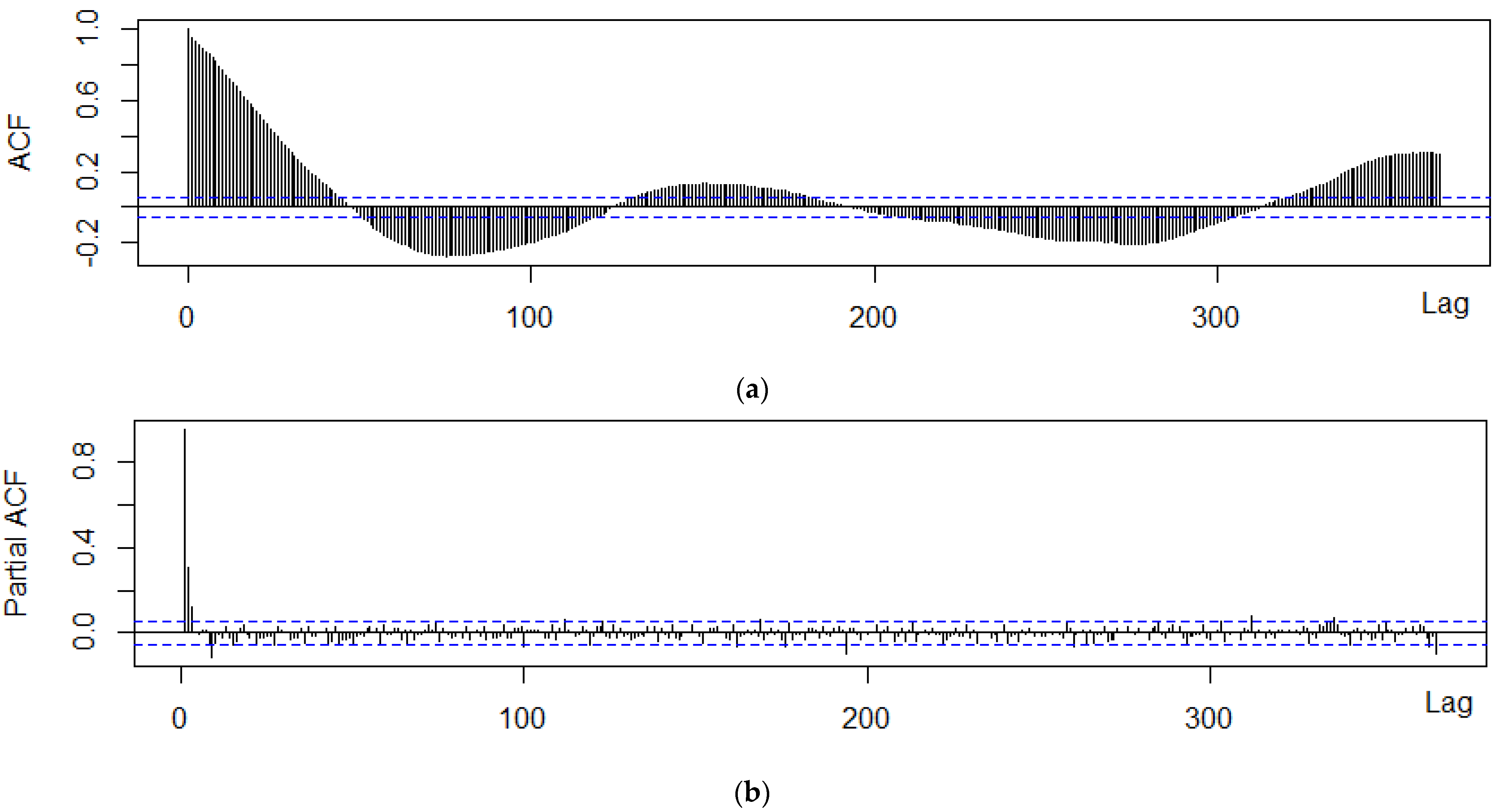
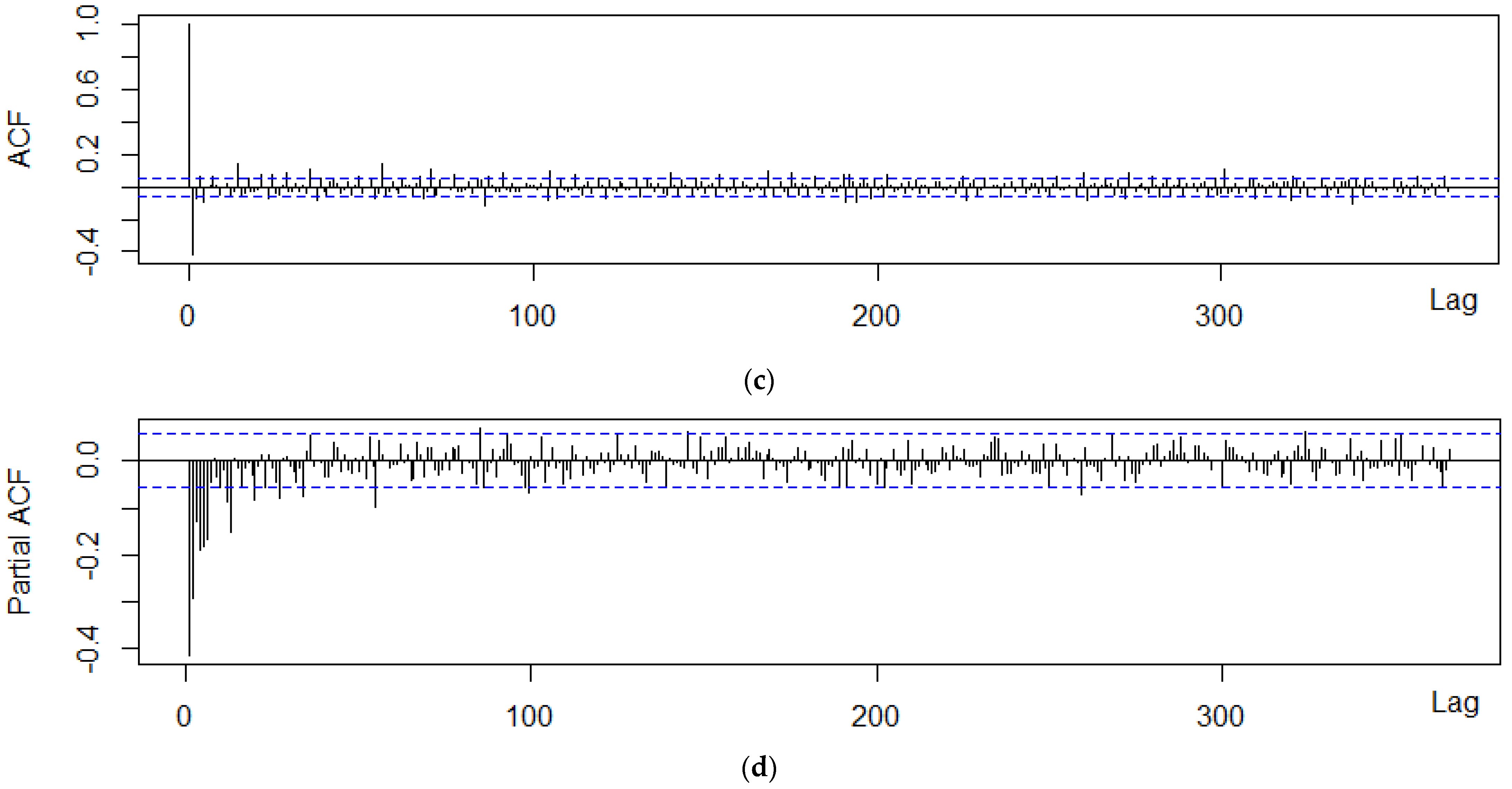
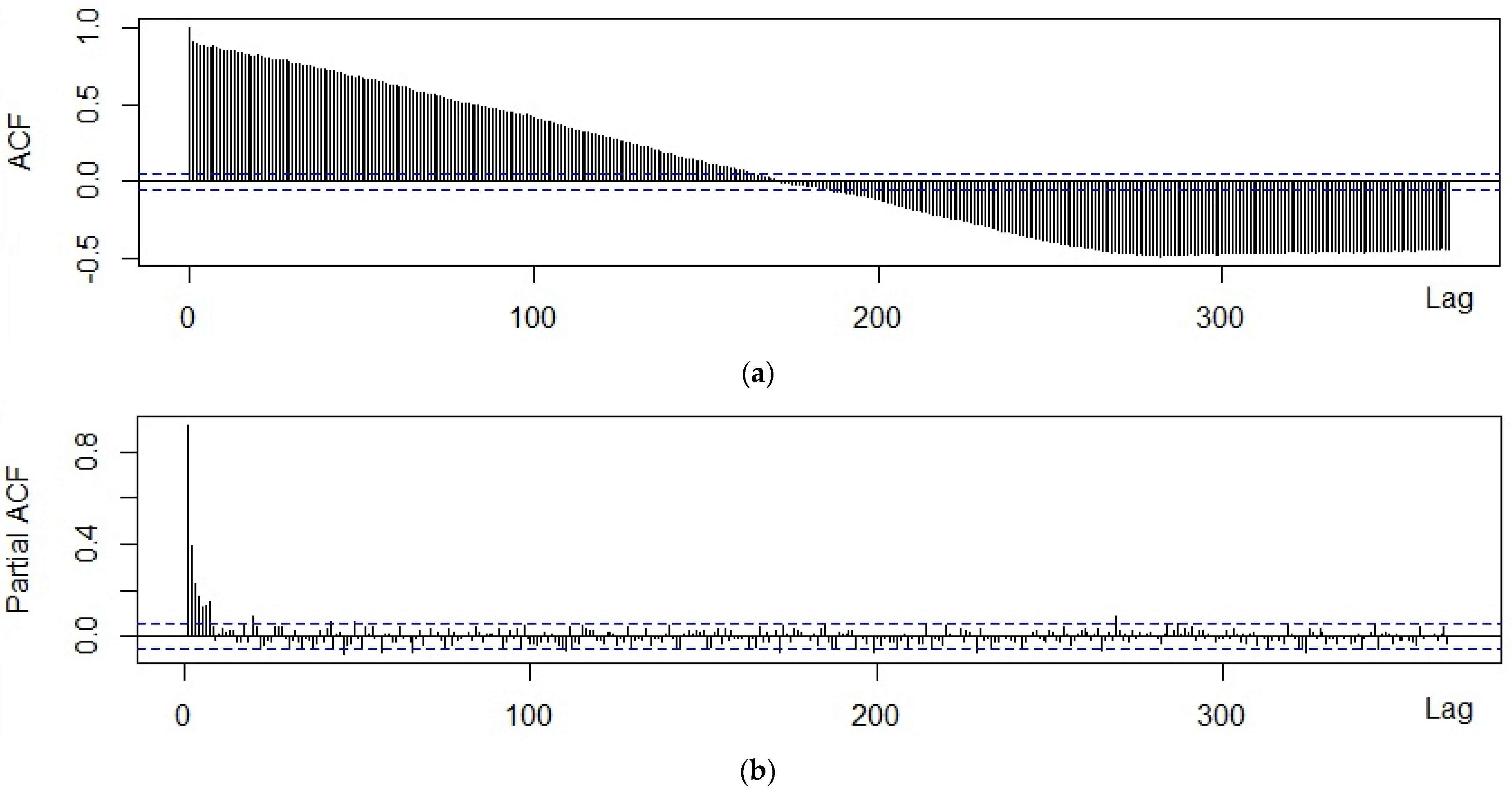
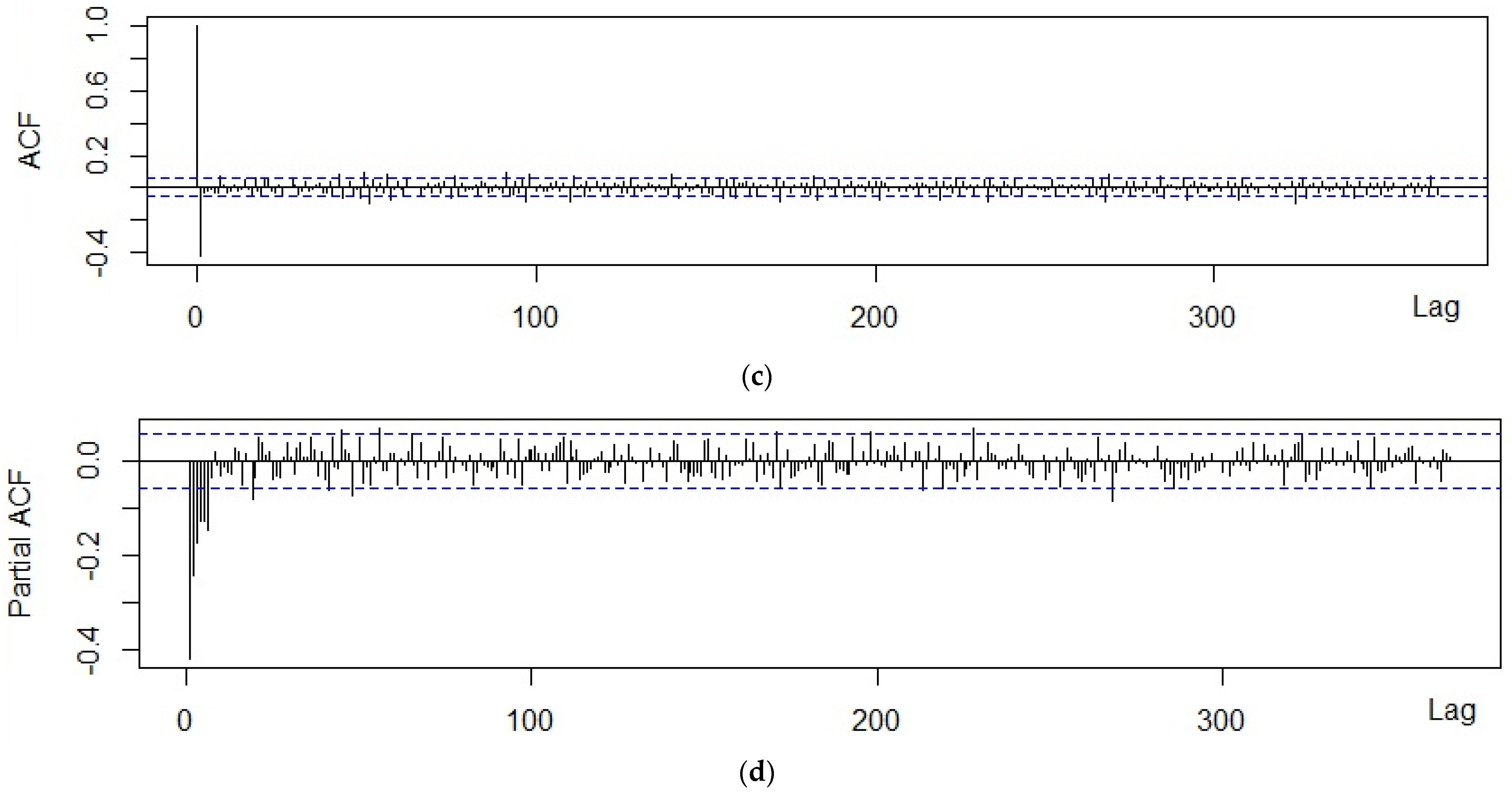
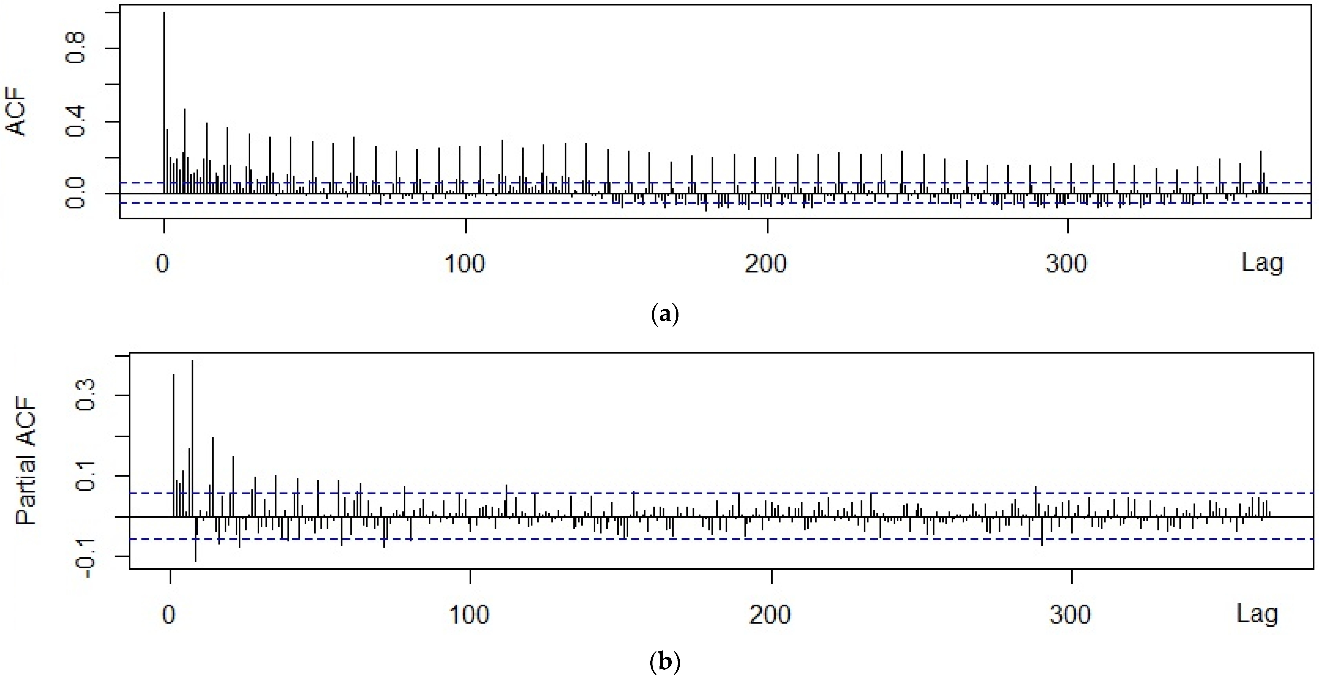
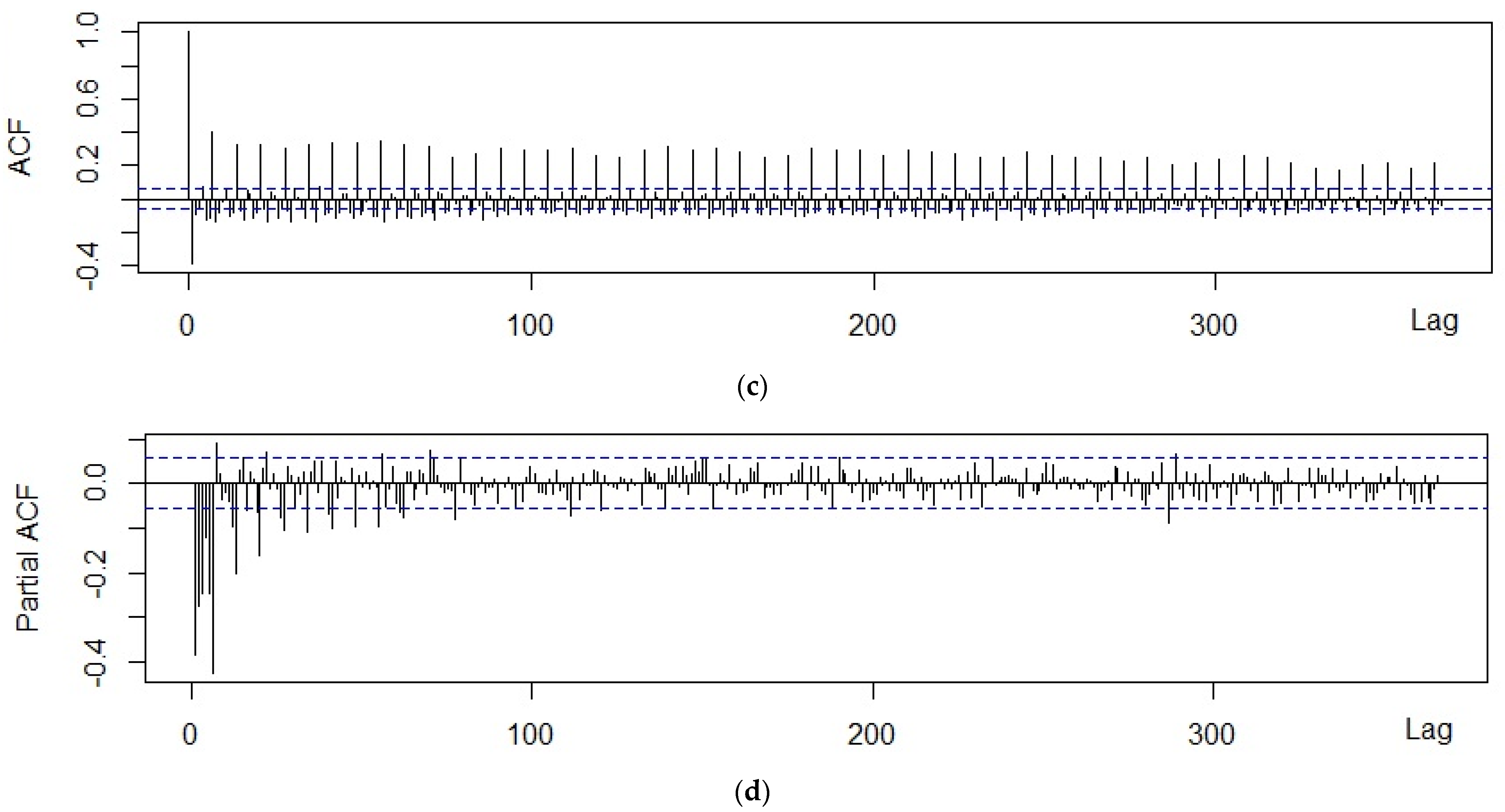
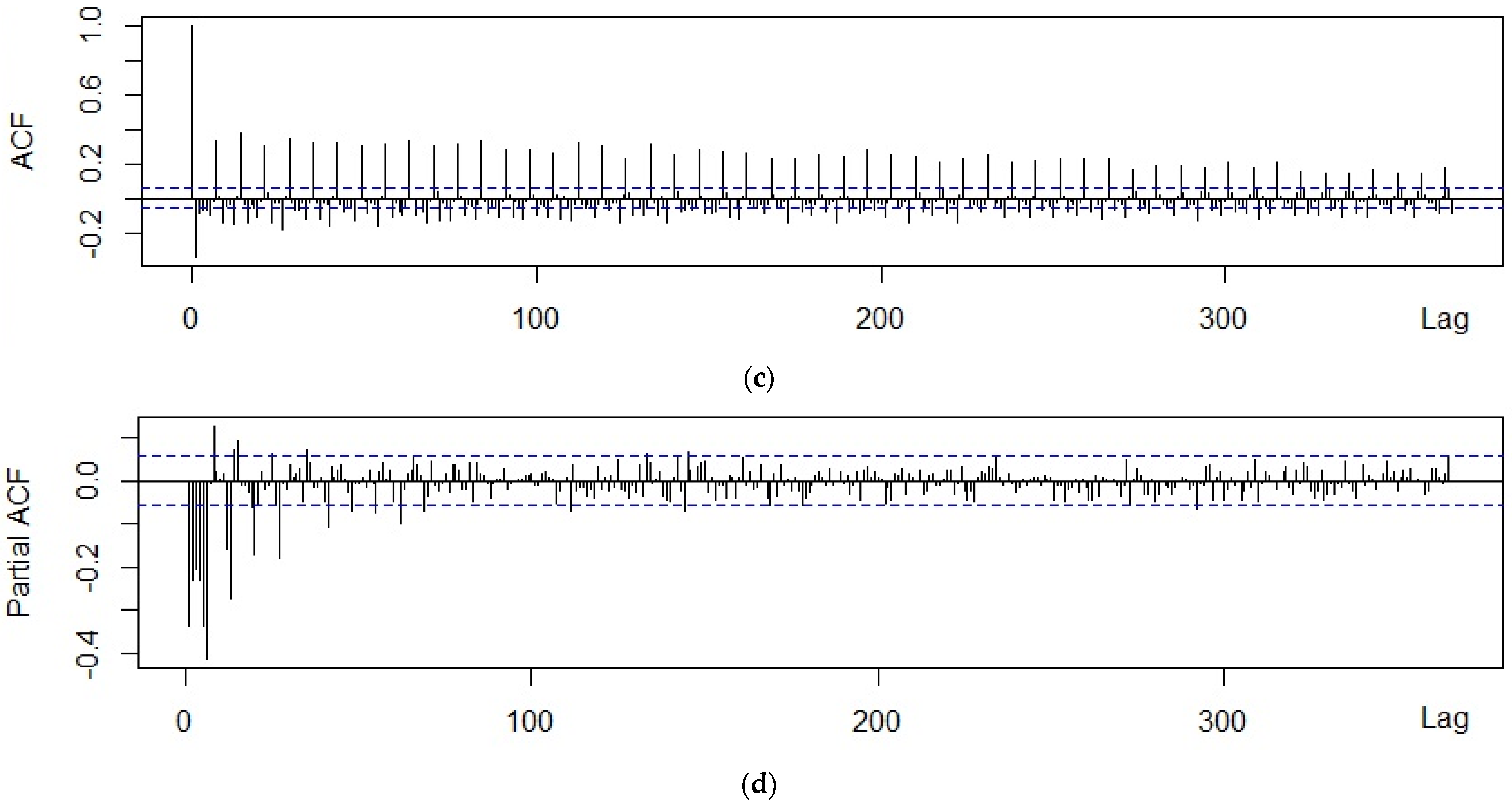
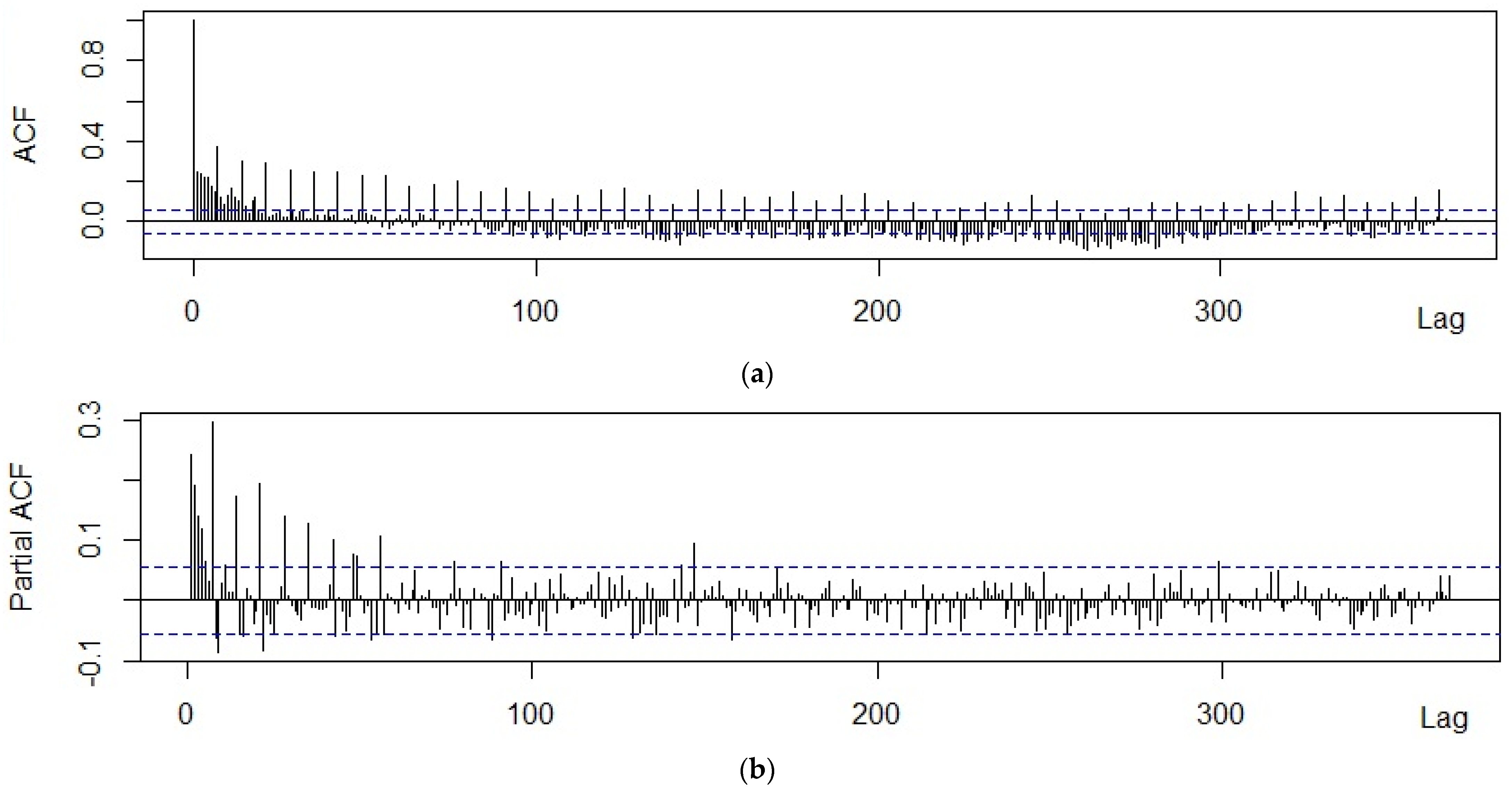
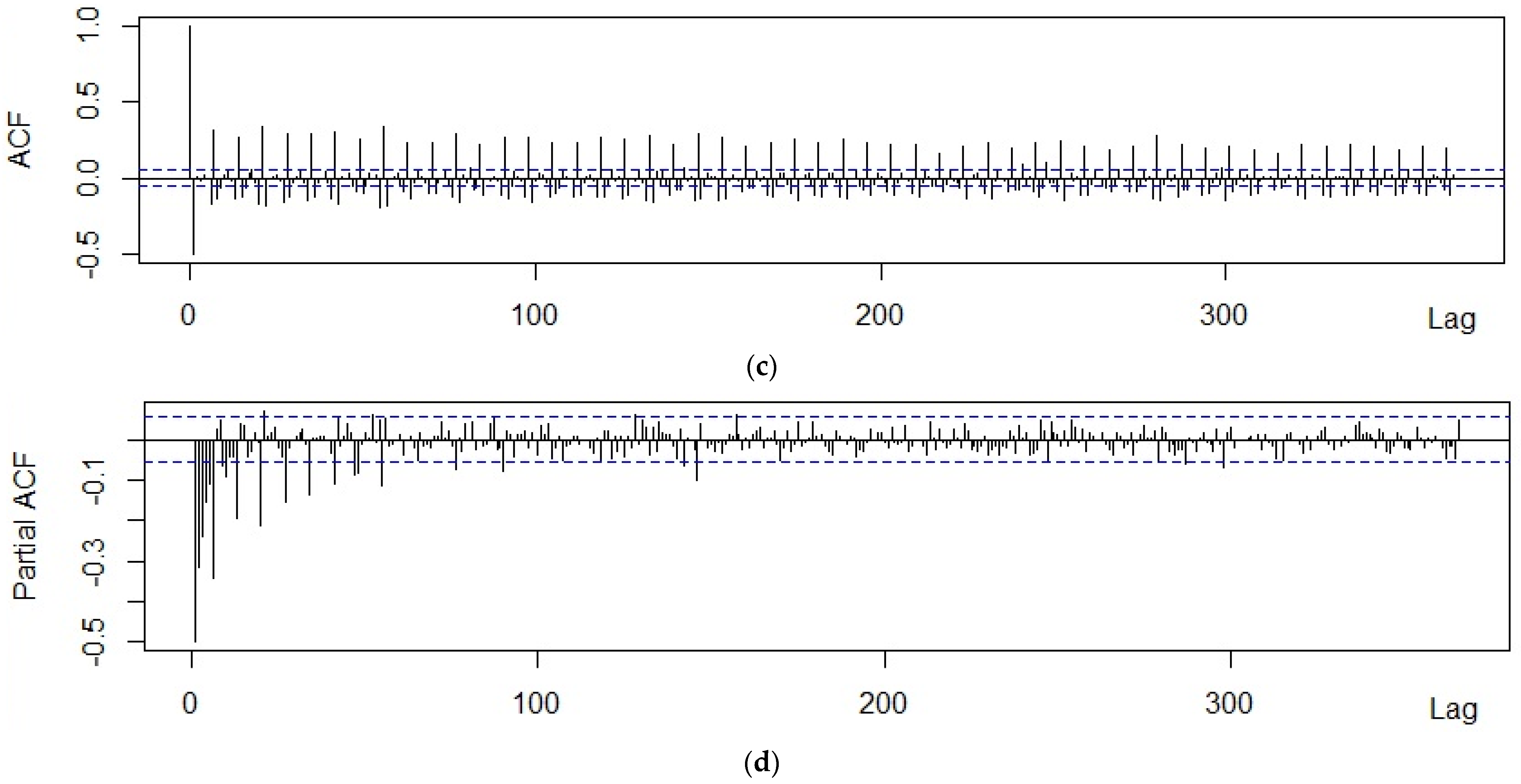
In order to take the seasonality of the data into account, we analyzed the shape of the time series as well as both autocorrelation function (ACF) and partial autocorrelation function (PACF) graphs [
36,
37]. The ACF expresses the internal correlation between observations in a time series separated by different lags as a function of time lag, and the PACF describes the direct relationship between an observation and its lag. These indicators represent correlations of the residuals that remains after removing the effects, which are explained by the earlier lag(s). The ACF graph helps in choosing the appropriate values for the ordering of moving average terms and the PACF graph is useful for the autoregressive terms [
38].
In addition, we conducted the most appropriate statistical tests, such as Welch’s ANOVA test, the Friedman Rank test, the QS test, Ollech and Webel’s combined seasonality test. The last test is based on both the QS test and Kruskal–Wallis test that are calculated on the residuals of auto-ARIMA without seasonality. For example, the seasonality is not rejected by Ollech and Webel’s test in a time series in case the p-value of the QS test is less than 0.01 or that of Kruskal–Wallis test is less than 0.002.
The analysis was carried in R by using ‘sf’, ‘spdep’, ‘ape’, ‘seastest’ and ‘tseries’ packages, as well as GeoDA software.
4. Discussion
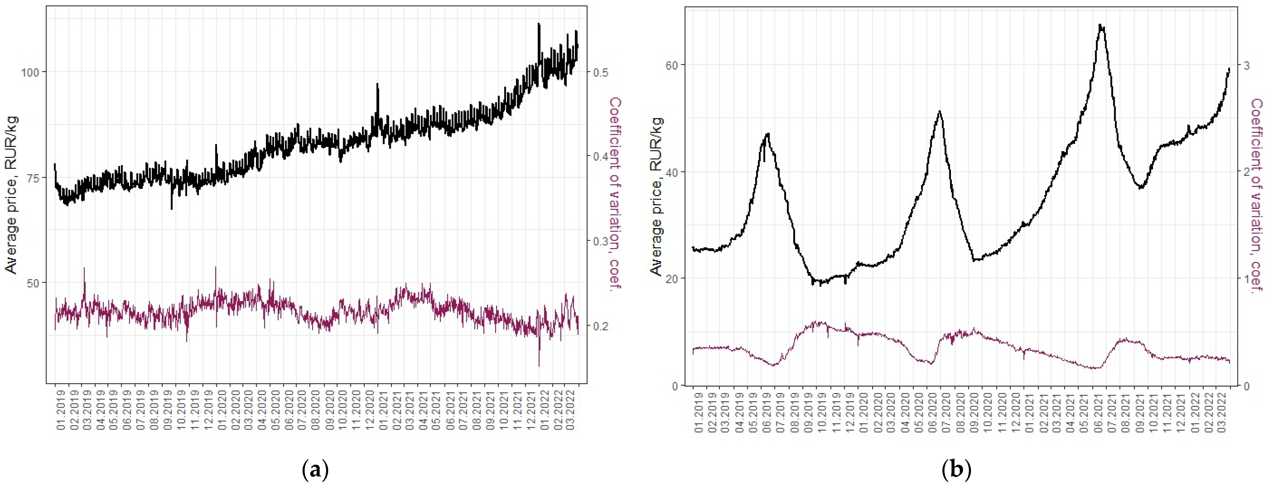
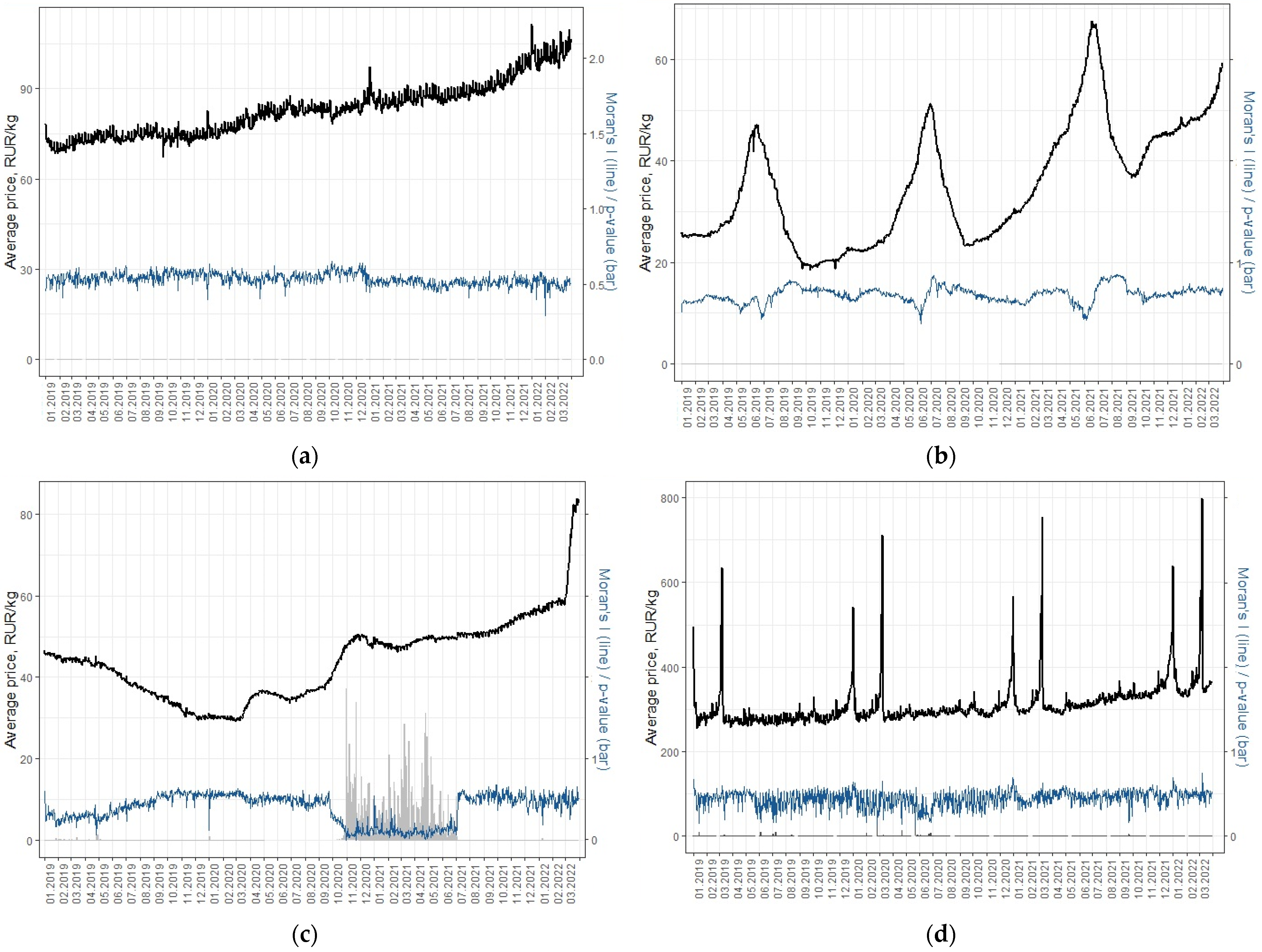
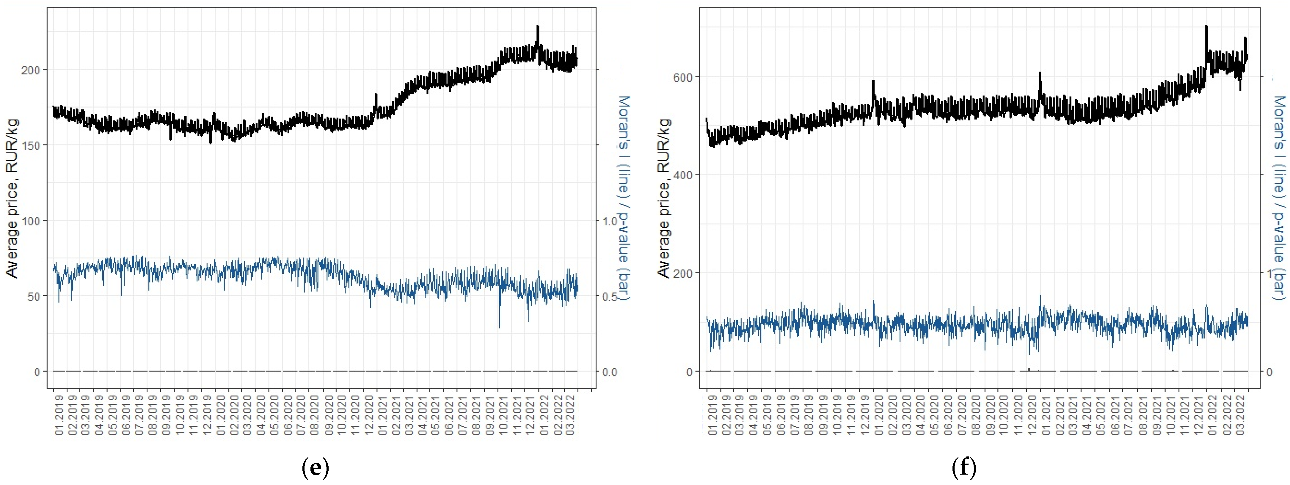
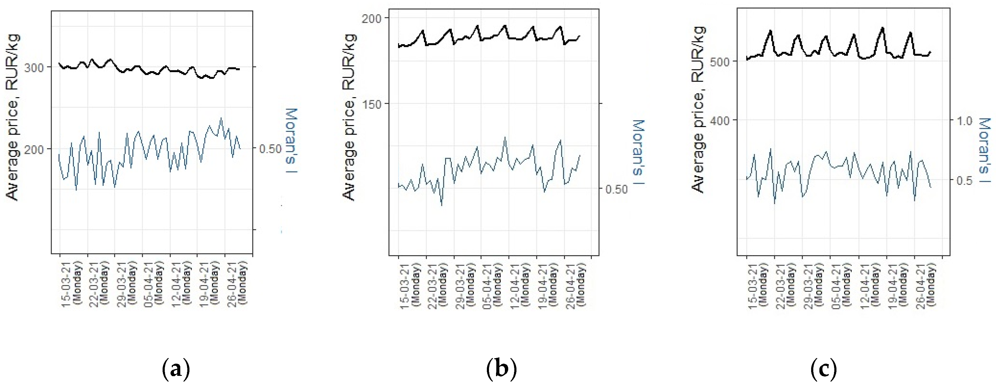
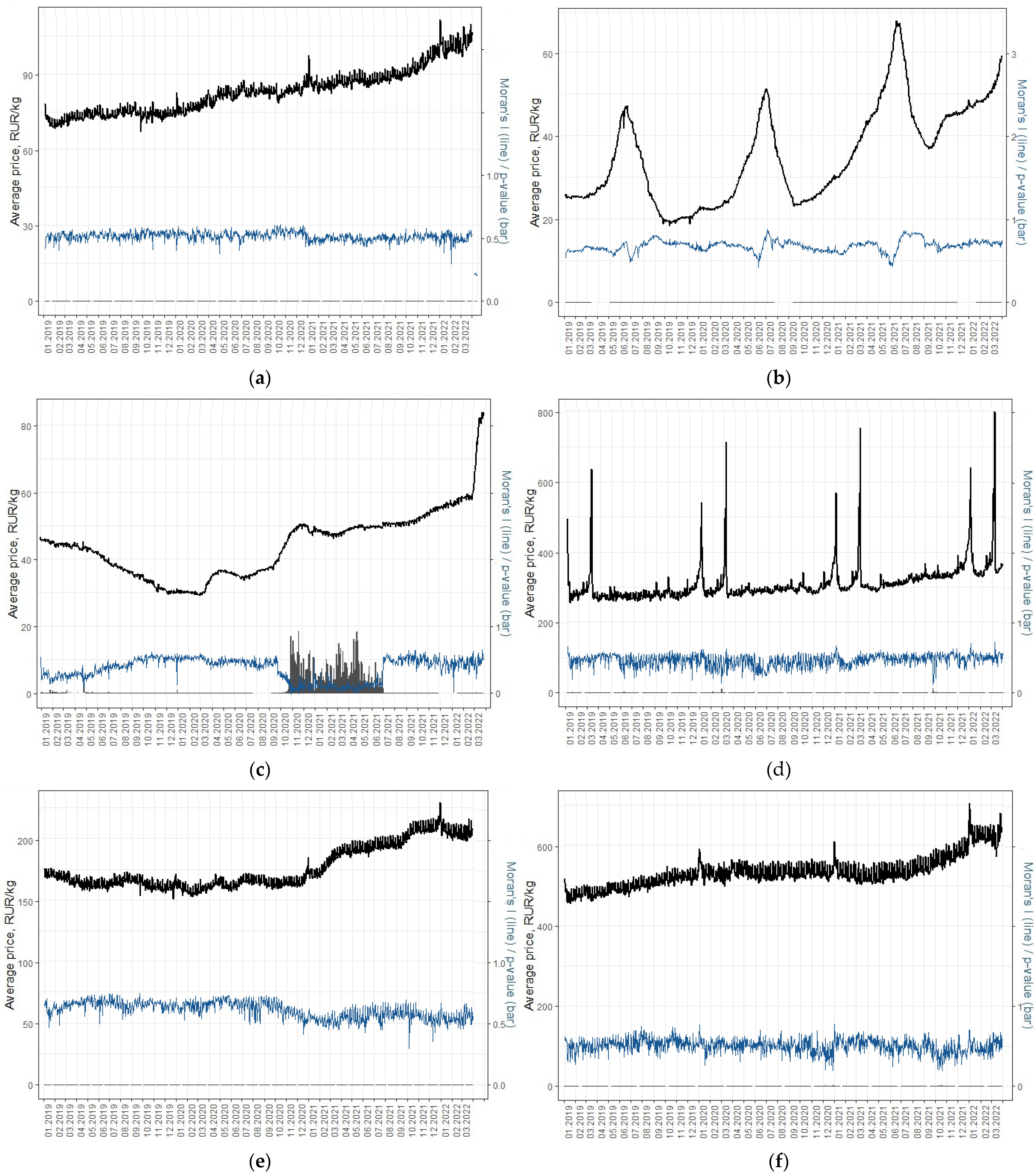
The analysis was carried out on the price data of six product categories. We estimated indicators such as spatial variation (coefficient of variation) and spatial autocorrelation (Moran’s I). The dynamics of the price of product categories varies. Each category’s dynamics is driven by its own characteristics, which affect the resulting estimates of variation and spatial autocorrelation (
Figure 1 and
Figure 2 and
Figure A1).
This corresponds fairly well to the results of the previous studies showing that estimates of spatial variation and convergence of regions for a particular group of products may not coincide with estimates for a general price index [
3,
11]. Moreover, the spatial relationships may vary for different groups of goods [
23], also due to different policies for price regulation in the regions [
22]. Thus, the research on separate product categories might benefit with deeper understanding of the spatial dependence of prices, since many of the categories often demonstrate particular spatial price dynamics.
The calculations show that the regional price variation and spatial autocorrelation vary not only across the product categories, but also across time. The estimates calculated for one period may not always accurately characterize the real spatial dependence. We would like to discuss certain factors that may lead to the variability of the estimates in time.
4.1. Holidays and Special Events
As mentioned earlier, this study is based on the average price of sold products, actually paid by the consumer at the time of purchase and registered by cash registers. In this regard our approach differs from one used to calculate the CPI (consumer price index) [
29]. However, this approach has an important drawback: the consumer prices are often subject to consumer sentiments, since the average price of sold products depends on the structure of sales and the prices. Consumer spending for some products is known to be uneven during the year with peaks around holidays [
33]. This is a reason for the average price not to follow the change in prices evenly. The effect is especially important, e.g., for Candies.
On New Year’s Eve and right before International Women’s Day (8 March) the sales of sweets and candies increase significantly in Russia, not only in terms of volume of sales. Moreover, the consumers tend to buy more expensive sweets at that time. As a result, there are peaks for average sweet prices during these holidays (
Figure 1d,
Figure 2d and
Figure A1d).
This effect is evident even though many chains promote and discount sweets in this period. The prices for Pasta and Butter are also higher on New Year’s Eve (
Figure 1 and
Figure 2). Meanwhile, the change in prices for other product categories is not significant.
Usually, the highest regional variation of prices is observed during these periods. For example, the highest values of spatial variation (
Table 2) correspond to the New Year’s holidays (for Sugar on 1 January 2020; Pasta on 31 December 2019) and for International Women’s Day (for Candies on 8 March 2022).
Spatial autocorrelation of prices on these holidays is also usually quite high for all product categories except for Sugar. The highest value of spatial autocorrelation (Moran’s Ib = 0.75) was recorded on 8 March 2022, for Candies.
4.2. Weekly Cycles
Our study also revealed a weekly cyclicity in spatial autocorrelation. However, the results remain debatable.
The cyclicity of the average price is evident (
Figure 1 and
Figure 2 and
Figure A1). The average price reaches highest values on Sunday. The cycles of the Moran’s I are not so evident. However, we noticed that Moran’s I is mostly lower on Monday than the day before (
Figure 4). The only exception are public holidays.
This cyclicity can be explained by various factors. As Leclair et al. argue, the consumers might prefer going shopping on certain days of the week and retailers might offer a reduced price on the days that are less busy [
29]. This might apply well to Russia, even though the study of Leclair et al. showed very little variation of prices by the day of the week, at least for certain products. Another reason for the observed cyclicity might be the alignment of ’consumers feelings’ [
33], as people tend buying goods that are more expensive and in larger amounts on the weekend. There were also discussed and identified several examples of co-movement of prices in spatially separated markets in Russia [
22]. Interestingly, in some regions the purchase of cheaper brands of goods is more pronounced on Monday. spatial prices for Butter may differ on Sunday and Monday (
Figure 5).
The number of regions for which the price of Butter differs from that in neighboring regions is larger on Monday than on the weekend (
Figure 5). We notice this effect weekly throughout the whole study period (excluding holidays) and therefore consider it as non-accidental.
4.3. Annual Seasonality
The price level and supply of some food products, mainly vegetables and fruits, is annually variable, depending largely on seasonal production. This applies to potatoes, for example [
38]. Prices tend to drop during the harvest period and rise from around New Year’s Eve onwards, when last year’s stocks are over.
Russia has several climatic zones. The period of harvest is earlier in some regions than in the others. Moreover, vegetables are not grown in some regions at all due to cold weather, causing additional effects on the spatial correlations of changes in prices.
The spatial variation and spatial autocorrelation usually decrease when the prices rise because of dwindling stocks from the previous year (
Figure 1 and
Figure 2 and
Figure A1). At the same time, the quality/availability of warehouse storage and the volume of stocks in regions vary significantly, which results in fragmentation of the national market. In this case, the Moran’s I values drop, indicating a higher price difference between neighboring regions. The effect of the season is important, e.g., for Potatoes.
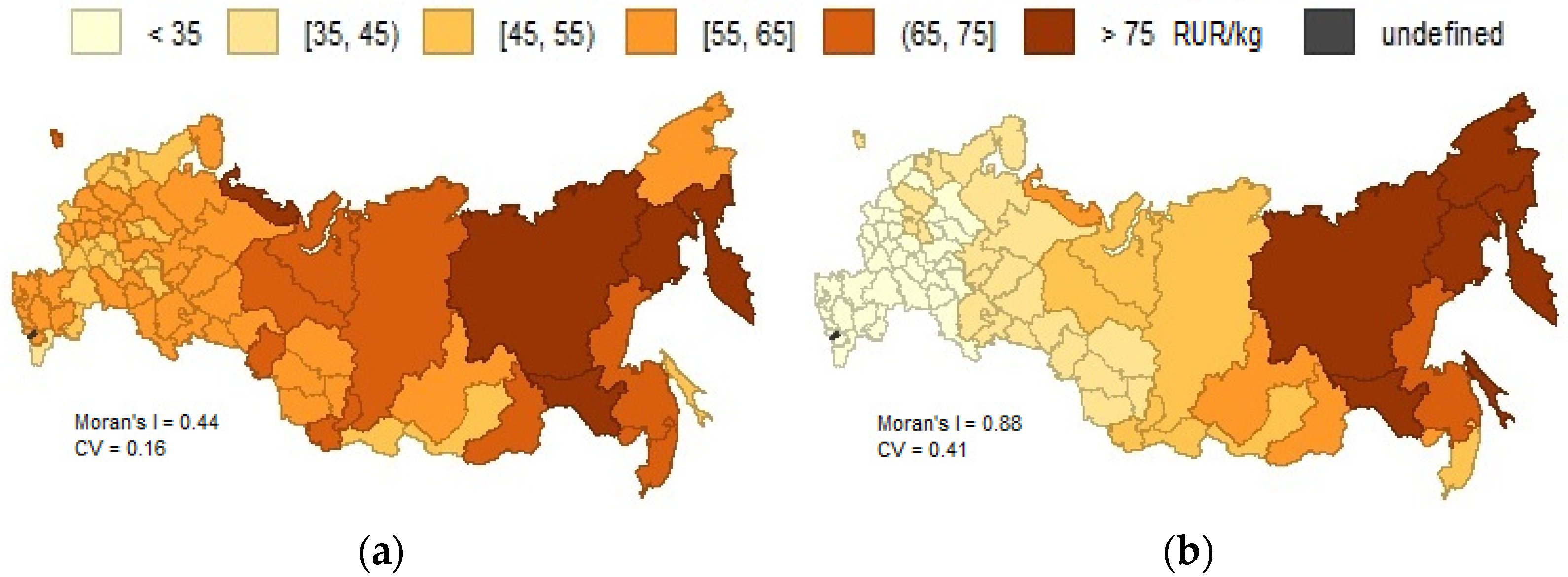
With the beginning of the first harvests, the spatial variation between regions increases. The prices start declining in the south, while they remain relatively high in the north. Spatial variation and spatial autocorrelation grow (Moran’s I
b = 0.88 on 10 August 2021, compared to Moran’s I
b = 0.44 on 5 June 2021) as a result, because the regions are geographically structured according to their specialization in agriculture (
Figure 6a,b).
The gradual change in prices is associated with the speed of filling the market with new crop potatoes. In the north, due to more expensive storage and delivery conditions, prices nearly always remain high [
22]. Therefore, the spatial variation does not decrease, at least not significantly. At the same time, the spatial autocorrelation decreases due to the fragmentation of the market (uneven reductions in stocks and increases in potato prices in regions).
4.4. External Shocks and State Regulation of Prices
Prices for some products may also change under the influence of external shocks. One example is that of the COVID-19 pandemic, when the retail prices of maize and rice rose rapidly in African countries [
26]. Sugar and salt prices are traditionally most affected by external shocks in Russia. Sugar prices rose under both the first and the second COVID-19 pandemics waves (
Figure 1). Numerous research papers indicate a strict correlation between price spikes and peaks in spatial variance, as well as stronger fragmentation of the markets during price crises [
24].
Analysis of both sugar price dynamics, its spatial variation and autocorrelation indicates that the response to external shocks is mainly aligned across regions in Russia. The sugar prices began to rise during the first wave of COVID-19 in most regions, causing the variation to decrease and the spatial autocorrelation to remain almost unchanged. Perhaps, the fragmentation is more pronounced at lower geographic levels of data aggregation.
The situation changed, however, under the second COVID-19 wave. First, the amount of sugar produced exceeded the amount of consumption at that time. Therefore, prices were relatively low in 2019 and early 2020. Secondly, the sugar harvest in 2020 was low while the stocks were significantly reduced during the first wave of the pandemic. For these reasons, a sharp inflation in sugar prices was registered in the fall of 2020, amplified by the second wave of the pandemic. In many regions, the stocks were insufficient to meet the shock demand levels. Under such social conditions, the local authorities began to impose restrictions on both price-changes and exports of sugar, as among the ‘socially significant’ products in Russia. As a result, the price variation decreased, and the spatial correlations became insignificant. In the summer of 2021, the restrictions were lifted as promising news about the sugar harvest became known and prices stabilized quickly, forming a spatial price equilibrium (
Figure 2).
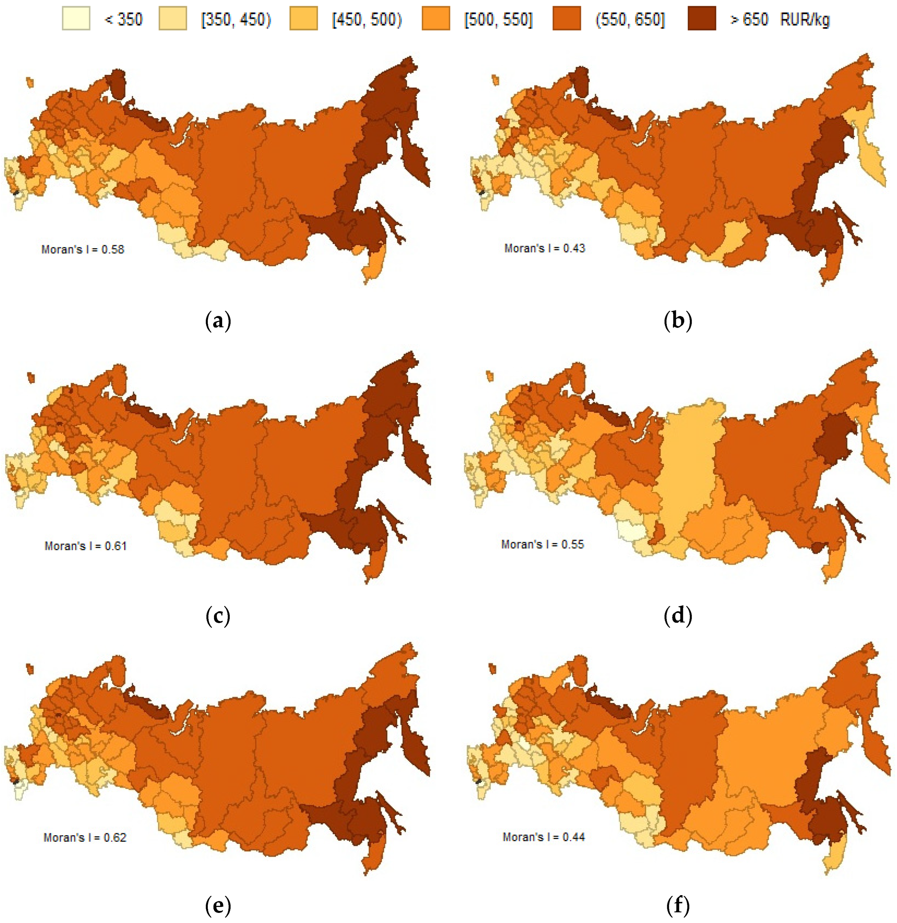
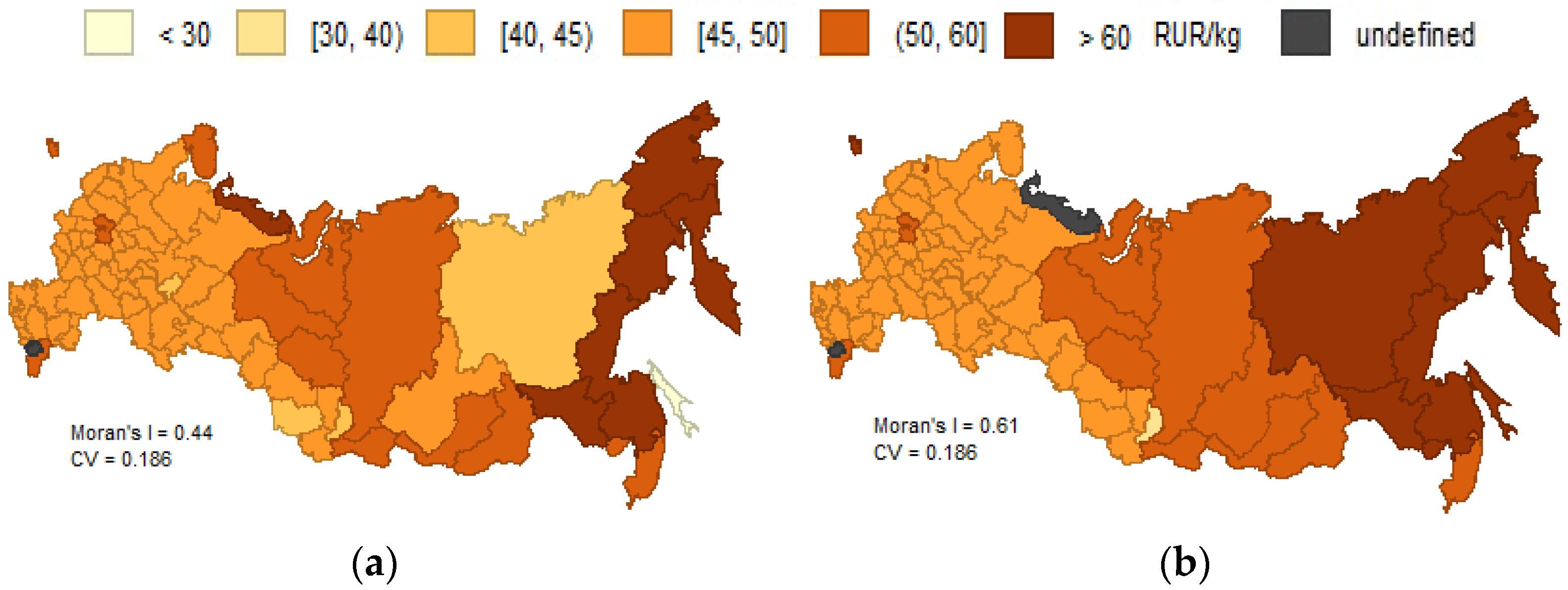
4.5. Spatial Variety vs. Spatial Autocorrelation
As our analysis showed, the change in spatial variety and spatial autocorrelation over time is not the same (
Figure 1 and
Figure 2 and
Figure A1). These are two different indicators: the growth of among them may not coincide with the growth of the other, and vice versa. The same level of a coefficient of variation (0.186) may well coexist both with high (Moran’s I
b = 0.61,
p-value < 0.001) and low (Moran’s I
b = 0.12,
p-value < 0.04) levels of spatial autocorrelation (
Figure 7).
In our view, these indicators can complement each other. Spatial autocorrelation can explain how chaotic the variation is and whether there are connections between neighbors. This is consistent with previous simulation results, which shows that the Moran’s I might show clustering [
40]. Therefore, it is important to expand the use of spatial autocorrelation methods in the study of regional price differences.
The calculation of Moran’s I using both binary contiguity matrix and inverse distance weights matrix showed that, in general, the binary matrix gives higher estimates of spatial autocorrelation (
Table 3). As it has been shown earlier the distance-based weighting criteria serve better for calculating the Moran’s I values, compared to contiguity-based criteria in terms of the capability of characterizing different forms [
40]. In our study, the difference between the results obtained for these two types of weights matrix is not large. At the same time, there are practically no differences in the dynamics of Moran’s I
b and Moran’s I
id indexes (
Figure 2 and
Figure A1).
5. Conclusions
We studied the spatial distribution of the prices of six product categories, namely Pasta, Potatoes, Sugar, Candies, Poultry meat and Butter based on the data available for the period from 1 January 2019, to 31 March 2022, (1186 days) in the context of 83 regions of Russia. The analysis showed that spatial variation and spatial autocorrelation change over time. Therefore, price analysis on low-frequency periodic data (one month or even a quarter) may not accurately reflect the general situation with the spatial distribution of prices. Changes in prices and their spatial relationship can be cyclical, determined by factors, such as holidays, weekends, and seasonal production. When price changes occur in regions simultaneously, the spatial autocorrelation does not change. A decrease in spatial autocorrelation is observed, however, when the market is fragmented. For example, on weekends, there is an aligned ‘feeling’ of consumers, determined by the will to purchase more expensive goods. Nevertheless, in the following days, prices in the regions may show a higher variation. For seasonally produced potatoes, there is a nearly permanent difference in prices in the north and south of the country all year around. We also revealed that the authorities/states influence the spatial autocorrelation of prices. The spatial autocorrelation was insignificant during the period of price regulation for Sugar.
We conclude that spatial price variation and spatial autocorrelation are complementary measures. Both are important for understanding the spatial equilibrium of prices. At the same time, there has been much more research on the analysis of spatial variation than the analysis of spatial autocorrelation. We hope our study will fill this gap at least partly.
However, our results remain debatable, due primarily to the study design. First, our calculations are based on the average price of products sold. The growth rate for average price differs from CPI, which takes the quality and structure of products into account. Several studies show that 97 percent of the variation in price levels across space in these indexes can be attributed to unobserved heterogeneity in the products [
28]. The design of an indicator must be considered when interpreting and comparing the results. At the same time, the advantage of focusing on the average price of goods sold is that it allows for a better understanding of consumer behavior. Secondly, we considered a limited range of factors of spatial price change and did not consider differences in the development of transport and storage infrastructure in the regions. At the same time, the spatial price equilibrium modeling framework emphasizes the importance of transportation costs between markets [
41]. Thirdly, there remain a question of an appropriate spatial weights matrix to model the economy of such a spacious and particular country as Russia. Both types of spatial weights matrix have pros and cons to consider.
This study is among the few in which the price analysis was calculated on daily data in the context of several product categories. The results show that the dynamics of prices and their spatial dependence are different in the context of product categories and time periods. More and more detailed datasets will be available for researchers as long as the data engineering processes and technologies develop. This would allow a better understanding of the speed and direction of price changes in the short term and therefore more precise targeting of food/product security measures on behalf of the state/authorities. We also expect to understand the spatial correlation processes in prices better as soon as better-detailed primary data become available in the advent of data lakes epoch. New efficient approaches for economic data analysis are already discussed [
42,
43]. We underline the importance of appropriate specification of economic models. The models on daily price changes would require a careful selection of independent factors besides of the time and space-lagged variables to increase the accuracy of predictions.


